The Growth of Brightest Cluster Galaxies and Intracluster Light Over the Past Ten Billion Years

Abstract

We constrain the evolution of the brightest cluster galaxy plus intracluster light (BCG+ICL) using an ensemble of 42 galaxy groups and clusters that span redshifts of $z=0.05-1.75$ and masses of M_500,c$=2\times 10^{13}-10^{15}$ M_⊙. Specifically, we measure the relationship between the BCG+ICL stellar mass M_⋆ and M_500,c at projected radii $10<r<100$ kpc for three different epochs. At intermediate redshift ($\bar{z}=0.40$), where we have the best data, we find M_⋆$\propto$M_500,c^0.48±0.06. Fixing the exponent of this power law for all redshifts, we constrain the normalization of this relation to be $2.08\pm 0.21$ times higher at $\bar{z}=0.40$ than at high redshift ($\bar{z}=1.55$). We find no change in the relation from intermediate to low redshift ($\bar{z}=0.10$). In other words, for fixed M_500,c, M_⋆ at $10<r<100$ kpc increases from $\bar{z}=1.55$ to $\bar{z}=0.40$ and not significantly thereafter. Theoretical models predict that the physical mass growth of the cluster from $z=1.5$ to $z=0$ within r_500,c is 1.4$\times$, excluding evolution due to definition of r_500,c. We find that M_⋆ within the central 100 kpc increases by $\sim 3.8\times$ over the same period. Thus, the growth of M_⋆ in this central region is more than a factor of two greater than the physical mass growth of the cluster as a whole. Furthermore, the concentration of the BCG+ICL stellar mass, defined by the ratio of stellar mass within 10 kpc to the total stellar mass within 100 kpc, decreases with increasing M_500,c at all $z$. We interpret this result as evidence for inside-out growth of the BCG+ICL over the past ten Gyrs, with stellar mass assembly occuring at larger radii at later times.

1 Introduction

In the paradigm of hierarchical assembly, massive halos are assembled from smaller halos. The most massive galaxies at any epoch represent the culmination of this process and are expected, as a class, to continue to grow from the accretion of smaller galaxies up to the current time. Brightest cluster or group galaxies (hereafter BCGs) trace the most overdense peaks in the matter distribution. Connected to the evolution of the BCG is the build-up of its extended stellar halo, the so-called intracluster light (hereafter ICL), which extends to hundreds of kpc (Oemler, 1976; Schombert, 1988; Gonzalez et al., 2005; Zibetti et al., 2005). The rate of growth of the sum of these two components (hereafter BCG+ICL), and the time of ICL formation relative to that of the BCG, thus represent important benchmarks for models of cluster and massive galaxy formation.

While the physics underlying predictions of massive galaxy growth is straightforward, comparisons of the rate of BCG+ICL growth between models and observations, and even among the observations themselves, yield disparate results. For example, De Lucia & Blaizot (2007) used semi-analytic models based upon the Millennium simulations to track the stellar mass growth of BCGs via merger trees, finding a factor of three growth since $z=1$. More recent semi-analytic models that also include the ICL (Contini et al., 2014; Contini et al., 2018) find that ICL growth is delayed compared to growth of the BCG, resulting in an even larger growth of the BCG+ICL since $z=1$. In contrast, observational studies of BCG growth typically have found less stellar mass evolution, from essentially none (Whiley et al., 2008; Collins et al., 2009; Stott et al., 2010) to 1.3 to 2$\times$ over a comparable redshift range in more recent papers (Lidman et al., 2012; Lin et al., 2013; Bellstedt et al., 2016; Zhang et al., 2016). A challenge in comparing the observational results is the use of different apertures to define the BCG stellar mass (Burke et al., 2000; van Dokkum et al., 2010; Zhang et al., 2016), leading to the inclusion of more or less of the extended ICL component. Any systematic discrepancy with theory may arise from a failure to account for ICL stars at larger radii (Zhang et al., 2016), particularly given the expected delayed growth of the ICL.

If the late-time build-up of the BCG+ICL component is such that the ICL is assembling faster than the BCG (e.g. Contini et al., 2014; Contini et al., 2018), then one will observe “inside-out" growth in the stellar mass distribution. With observations of the radial profile of the BCG+ICL over a range of redshifts, it is possible to determine how the concentration of the stellar mass changes over time and therefore to test the inside-out scenario.

Measurements of the BCG+ICL radial profile are technically challenging. and consistent from $\bar{z}=0.4$ to $\bar{z}=0.10$. While the extended halo of the BCG+ICL often dominates the total stellar light within the central few hundred kpc (e.g. Gonzalez et al., 2005, 2013; Zhang et al., 2019), it can be of extremely low surface brightness, far below that of the background sky. Meticulous control of systematics is thus required, even at low redshift. Cosmological dimming and a decrease in the stellar mass of the BCG+ICL with increasing redshift add to the challenge when measuring the BCG+ICL at higher redshift.

As a result, there are only a few measurements of the BCG+ICL  extending beyond the central $\sim 20$ kpc in clusters at $z\ga 1$ (Burke et al., 2012; Zhang et al., 2016; Ko & Jee, 2018). Burke et al. (2012) measured the ICL in a sample of six clusters at $z\sim 1$, finding that the stellar content with $\mu_{J}>22$ mag arcsec^-2 represents only $1-4$% of the total cluster luminosity within r_500,c and that it grows $2-4\times$ by the present day. Ko & Jee (2018) provides the only HST study of the ICL at $z>1$, arguing for modest growth based on their detection of a substantial ICL in MOO J1014+0038 ($z=1.24)$, which we also include in this study.

In this paper, we measure the BCG+ICL out to projected radii of 100 kpc, where the ICL dominates (Gonzalez et al., 2005; DeMaio et al., 2015), for 42 groups and clusters spanning a range of redshifts. This work includes new HST measurements of the BCG+ICL for seven clusters at $z\geq 1.24$ (mean redshift $\bar{z}=1.55$). We make no attempt to distinguish between the BCG and ICL components, constraining their sum instead. Thus, our results can be used to directly test models in which the BCG+ICL is determined within this aperture. We further quantify the BCG+ICL stellar mass within fixed physical apertures of 10 and 100 kpc, and within an annulus of 10 to 100 kpc, and use these data to constrain the radial dependence of the growth.

These data, in combination with our previous work, provide constraints on when and how the mass of the BCG+ICL was established as a function of cluster mass. In Section 2, we describe the high redshift HST cluster sample ($\bar{z}=1.55$), which we combine with lower-redshift systems at $\bar{z}=0.10$ and $\bar{z}=0.40$ to create a wide redshift baseline. Because these latter samples are both from our own previous work, the comparison across mass and redshift is as consistent and straightforward as possible. In Section 3, we summarize the reduction methods for the new high-redshift clusters and describe how we produce their surface brightness profiles out to $\thicksim$100 kpc. We present the results of our analysis in Section 4, including how the observed trend between the BCG+ICL stellar mass and the total cluster mass evolves and how the concentration of the BCG+ICL stellar mass evolves. We summarize our conclusions in §5. We use the WMAP9 cosmology ($H_{0}$=69.3 km Mpc^-1 s^-1, $\Omega_{m}=0.286$; Hinshaw et al., 2013) as in DeMaio et al. (2015, hereafter Paper I) and DeMaio et al. (2018, hereafter Paper II). Throughout this paper, $r$ refers to projected radius from the center of the BCG, r_500,c is radius within which the cluster overdensity equal to 500 times the critical density of the Universe at the cluster redshift, and M_500,c is the mass enclosed within this radius.

2 Sample

At low redshifts, we use a sample of 12 clusters drawn from Gonzalez et al. (2005, hereafter GZZ05) for which Gonzalez et al. (2013, hereafter GZZ13) derive M_500,c from XMM-Newton observations. These 12 clusters span the mass range 0.9$\times 10^{14}$  M_⊙ $<$ M_500,c$<$ 6$\times 10^{14}$ M_⊙ at $z<0.15$ ($\bar{z}=0.10$). GZZ05 fit their observed BCG+ICL surface brightness profiles out to $r>300$ kpc with two de Vaucouleur profiles. We refer the reader to their Table 4 for the best-fit parameters of each system. For these systems, we first transform the photometry from the Cousins magnitudes in GZZ05 to Sloan $i^{\prime}$ using the color correction of Jordi et al. (2006) for $R-I=0.5$ before computing the luminosities. We then use the $i^{\prime}$ absolute magnitudes and structural parameters to compute the BCG+ICL luminosities within fixed physical apertures (e.g. 10 kpc, 100 kpc), enabling comparison with aperture luminosities measured for the other subsamples described below. The M_500,c values from GZZ13 are derived from XMM-Newton X-ray temperatures, $T_{x}$, using the Vikhlinin et al. (2009) prescription.

At intermediate redshift, $0.29\leq z\leq 0.89$ ($\bar{z}=0.40$), we have 23 systems from Paper II. These clusters span a wide range in M_500,c, 3$\times 10^{13}$$-9$$\times 10^{14}$ M_⊙. Data for clusters with M_500,cabove 10¹⁴ M_⊙ are from the Cluster Lensing And Supernova survey with Hubble  (CLASH Postman et al., 2012), while data for the others originate from HST Program #12575 (PI: Gonzalez). Paper II provides more details on these intermediate-redshift systems. For this paper, we focus on the F160W surface brightness profiles out to 100 kpc. We use these profiles to find the total luminosity and the stellar mass content of the BCG+ICL in each system.

M_500,c values for all these systems are derived from X-ray temperatures, using the Vikhlinin et al. (2009) transformation, M_500,c$=M_{0}(T_{x}/5{\rm\ keV})^{\alpha}_{x}E(z)^{-1}$ with $M_{0}=3.02\pm$0.11$\times 10^{14}$ $h^{-1}$ M_⊙ and $\alpha_{x}=1.53\pm 0.08$. The CLASH sample all have published Chandra X-ray temperatures (Donahue et al., 2014, 2016). For the lower mass systems X-ray temperatures come from a mixture of Chandra and XMM-Newton data. There is a systematic offset for the derived cluster masses of systems with $k_{B}T_{x}>5$ keV due to calibration effects; Chandra  masses have been found to be $\thicksim$15% higher than those determined with XMM-Newton observations (Mahdavi et al., 2013; Schellenberger et al., 2015). To bring the M_500,c values of both the low-redshift sample of GZZ05 and our intermediate redshift sample to a common framework, we apply a correction factor of 15% to the GZZ13 masses. Final M_500,c values after all corrections are presented in Table 2.

We extend the redshift baseline of this sample with clusters from HST Programs #13677 & #14327 (PI: Perlmutter; hereafter the high-redshift sample). These programs were designed to observe high-redshift supernova in massive clusters at $z>1$ to constrain the time variation of dark energy. The clusters in the sample cover a similar mass range to the lower redshift samples (Figure 1). We use the F160W observations of 7 clusters from this program (Table 2), which all lie at $z\geq 1.24$ ($\bar{z}=1.55$). For IDCS J1426.5$+$3508 we supplement the Perlmutter HST data with F160W imaging from HST Program #12994 (PI: Gonzalez), as described in Mo et al. (2016).

Redshifts, BCG positions and cluster masses are compiled from the literature for the high-redshift systems as follows:

1. For SpARCS-J0330 and SpARCS-J0224  we use the redshifts and cluster centers of Nantais et al. (2016). For these two systems we use M_200,c values from Lidman et al. (2012). We convert the M_200,c masses to M_500,c assuming an NFW (Navarro et al., 1997) profile with a Duffy et al. (2008) concentration, using the Python package colossus (Diemer, 2015).

2. For SpARCS-J1049  we use the BCG position as defined in Webb et al. (2015). Webb et al. (2015) provide two estimates of this cluster’s mass. With richness as a mass proxy, they find the cluster mass within 500 kpc to be (3.8$\pm 1.2$)$\times 10^{14}$ M_⊙. Using the velocity dispersion from 27 members within 1.8 Mpc they find a virial mass of (8$\pm$3)$\times 10^{13}$ M_⊙. A more recent weak lensing analysis (Finner et al., submitted) yields M_500,c$=2.5\pm 0.9$$\times 10^{14}$ M_⊙. All subsequent analysis uses this weak lensing-derived M_500,c.

3. For SPT-CL J0205$-$5829, the BCG identification and M_500,c are based on values in Tables 1 and B1 of Chiu et al. (2016).

4. For XDCP J0044.0$-$2033, we identify the galaxy ID1 in Fassbender et al. (2014) as the BCG and use the M_500,c estimate derived from the Chandra X-ray temperature in Tozzi et al. (2015).

5. For MOO J1014+0038, we adopt cluster coordinates and M_500,c from Brodwin et al. (2015). The M_500,c measurement is based on the observed Sunyaev-Zel’dovich (SZ) signal obtained with CARMA.

6. For IDCS J1426.5$+$3508, we associate the BCG identified in Brodwin et al. (2016) as the cluster center. Additionally, we use the value of M_500,c they derived using the $Y_{x}-$M_500,c mass proxy.

See Table 2 and Figure 1 for cluster details of the entire composite sample, which includes redshift, M_500,c, and references for the photometry and masses.

Table 1: Composite Cluster Sample

Cluster	z	M500,c	Notes
		1014 [M⊙]
Low-redshift ($\bar{z}=0.10$)
Abell 2401	0.0578	0.95$\pm 0.1$	$a$
Abell S0296	0.0699	1.45$\pm 0.21$	$a$
Abell 3112	0.0759	3.23$\pm 0.19$	$a$
Abell 1651	0.0853	5.15$\pm 0.42$	$a$
Abell 2955	0.0945	0.99$\pm 0.11$	$a$
Abell 4010	0.0963	2.41$\pm 0.18$	$a$
Abell 2984	0.1044	0.95$\pm 0.1$	$a$
Abell 2811	0.1082	3.59$\pm 0.28$	$a$
Abell S0084	0.1087	2.37$\pm 0.24$	$a$
Abell 0122	0.1127	2.26$\pm 0.19$	$a$
Abell 2721	0.1149	3.46$\pm 0.32$	$a$
Abell 3693	0.1237	2.26$\pm 0.23$	$a$
Intermediate-redshift ($\bar{z}=0.40$)†
Abell 611	0.288	3.66$\pm 0.25$	$b$
MS2137$-$2353	0.313	2.31$\pm 0.18$	$b$
XMMXCS J022045.1$-$032555.0	0.33	0.65${}_{-0.15}^{+0.27}$	$b$
RX J1532$+$3021	0.345	2.04$\pm 0.23$	$b$
RX J2248$-$4431	0.348	7.06$\pm 0.52$	$b$
MACS1931$-$2635	0.352	2.75$\pm 0.25$	$b$
MACS1115$+$0129	0.352	3.60$\pm 0.28$	$b$
SG 1120$-$1202$-$4	0.3688	0.80${}_{-0.41}^{+0.49}$	$b$
XMMXCS J011140.3$-$453908.0	0.37	0.60${}_{-0.15}^{+0.22}$	$b$
SG 1120$-$1202$-$2	0.3704	0.33${}_{-0.09}^{+0.15}$	$b$
SG 1120$-$1202$-$1	0.3707	0.49${}_{-0.14}^{+0.24}$	$b$
SG 1120$-$1202$-$3	0.3713	0.36${}_{-0.15}^{+0.37}$	$b$
RX J1334.0$+$3750	0.384	0.33${}_{-0.12}^{+0.39}$	$b$
MACS1720$+$3536	0.391	2.63$\pm 0.24$	$b$
MACS0429$-$0253	0.399	2.26$\pm 0.25$	$b$
MACS0416$-$2403	0.42	3.14$\pm 0.51$	$b$
MACS1206$-$0848	0.44	5.43$\pm 0.46$	$b$
MACS0329$-$0211	0.45	3.41$\pm 0.33$	$b$
RX J1347$-$1145	0.451	9.38$\pm 0.56$	$b$
MACS1311$-$0310	0.494	2.09$\pm 0.22$	$b$
MACS1149$+$2223	0.544	3.67$\pm 0.58$	$b$
MACS2129$-$0741	0.57	3.81$\pm 0.78$	$b$
CL J1226$+$3332	0.89	6.08$\pm 1.89$	$b$
High-redshift ($\bar{z}=1.55$)
MOO J1014$+$0038	1.24	3.40$\pm 0.40$	$c,d$
SPT-CL J0205$-$5829	1.32	5.65$\pm 1.40$	$c,e$
XDCP J0044.0$-$2033	1.58	2.8${}_{-0.6}^{+0.8}$	$c,f$
SpARCS-J0330	1.6	1.47${}_{-1.0}^{+1.5}$	$c,g$
SpARCS-J0224	1.63	0.26${}_{-0.1}^{+0.3}$	$c,g$
SpARCS-J1049	1.7	2.5$\pm 0.90$	$c,h$
IDCS J1426.5$+$3508	1.75	2.6${}_{-0.5}^{+1.5}$	$c,i$

• $a$ Photometry from Gonzalez et al. (2005) and masses from Gonzalez et al. (2013), $b$ Photometry from DeMaio et al. (2018), masses from Postman et al. (2012), $c$ Imaging from HST Programs #13677 & #14327, $d$ M_500,c  from Brodwin et al. (2015), $e$ M_500,c from Chiu et al. (2016), $f$ M_500,c from Tozzi et al. (2015), ^g Mass converted from M_200,c in Lidman et al. (2012), ^h Mass from Finner et al. (submitted), ⁱ M_500,cfrom Brodwin et al. (2016), ^† Computed excluding CL J1226+3332.

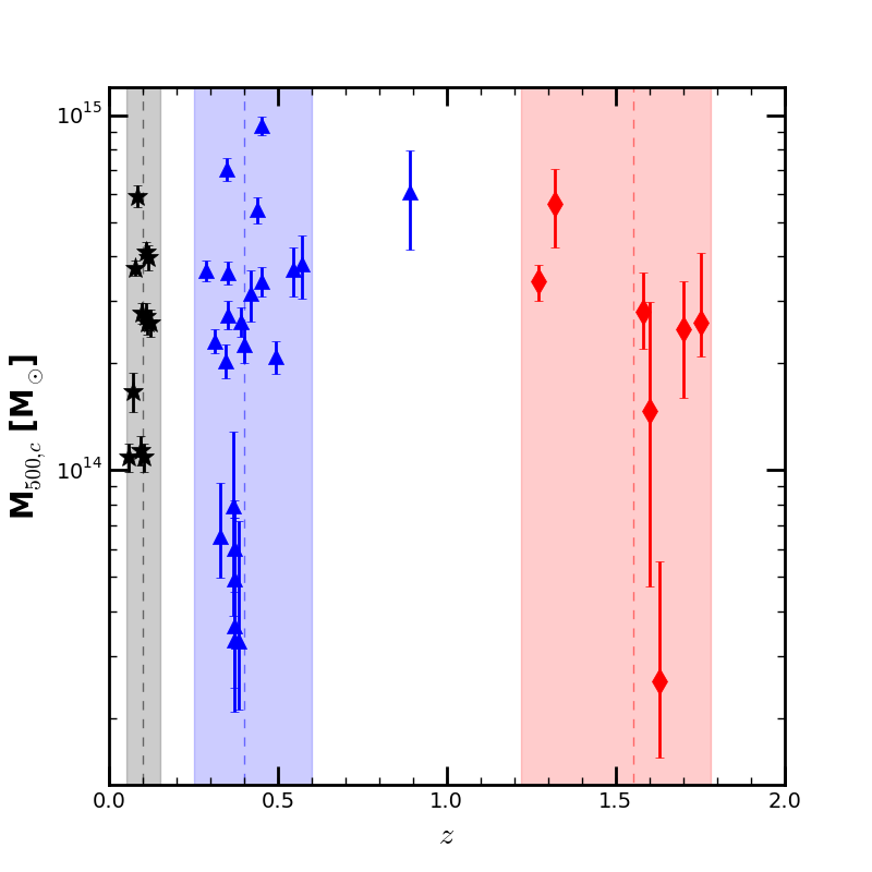
Figure 1: Cluster mass and redshift distribution of complete sample with low-redshift sources from GZZ05 (black stars), intermediate redshift systems from Paper II (blue triangles) and high-redshift clusters (red diamonds). The dashed vertical lines denote the mean redshift for each subsample, while the shaded regions indicate the redshift range of each subsample used to compute the mean redshifts. For the intermediate redshift sample, we exclude the cluster CL J1226+3332 at $z=0.89$ from subsequent analysis because its redshift is far from the mean of the sample and we lack other clusters at comparable redshift. from subsequent analysis Quoted M_500,c values are primarily derived from the X-ray temperature mass proxy using the Vikhlinin et al. (2009) prescription. All M_500,c values, literature sources, and mass proxies are listed in Table 2.

3 Reduction

We follow the same reduction procedure as in Paper II for the F160W imaging of the high-redshift sample, with one exception. We do not apply a $\delta$-flat to each input image before drizzling the data into a final science image for each epoch of observations because this is a sub-dominant systematic for the current analysis. The pixel-to-pixel rms variation in the pipeline flat fields is at the level of $\thicksim$0.5%. This level of photometric uncertainty does not dominate our error because we measure both the sky and BCG+ICL brightness over large areas and so the impact of local flatness variation is dramatically reduced. Any pixel-to-pixel correlations due to large-scale flatness variations across the detector are folded into our background measurement, which quantifies the uncertainty in the background as a function of position. More details on this method of constraining the flatness and background uncertainties are provided below.

We drizzle each epoch of data separately and then median combine all epochs of a given cluster into a final science image. This separate treatment of observations by epoch allows us to constrain the systematic variation in the background as a function of observation date. Of the seven high redshift clusters only the IDCS J1426.5$+$3508 field includes foreground stars that are projected within 100 kpc of the BCG. These two stars are fairly faint ($\sim 19-20$ mag in F160W), and masking is sufficient to ensure that light from the extended wings of the PSF does not significantly impact the observed BCG+ICL luminosity.

Finally, we perform source masking and background determination as in Paper II. We identify sources with Source Extractor (Bertin & Arnouts, 1996) and we mask all sources beyond 7″ of the BCG to 3 times the semi-major and semi-minor axis of the Source Extractor catalogs. Within 7″ we manually extend all mask radii to ensure that no remaining light from other stars and galaxies contributes to the BCG+ICL flux.

The cluster cores of XDCP J0044.0$-$2033 and SpARCS-J1049 are clear ongoing mergers. For these two systems we test how differences in masking at the cluster core affect the measured luminosity within $r<100$ kpc by comparing flux measurements from a series of differently masked images. At one extreme we mask all pixels that are associated with compact, high surface-brightness features. For example, in the case of SpARCS-J1049’s ’beads on a string’ morphology (Webb et al., 2015) all bright knots (beads) are masked. In the less restrictive masking regime we leave pixels unmasked if they are clearly associated with a distinct tidal feature or are irregular in shape and deeply embedded in the bright BCG envelope. As an example, we show an unmasked image and both masking schemes for SpARCS-J1049 in Figure 2. For SpARCS-J1049  differences in masking affect the total measured luminosity within 100 kpc by only 4%. For XDCP J0044.0$-$2033  the difference in the measured BCG+ICL luminosity within 100 kpc due to these differences in masking is 10%. We use the less-extensive masking schemes throughout our analysis and incorporate the uncertainty in flux due to masking difference into the quoted luminosity and stellar mass measurement uncertainties.

A B C

Figure 2: We test the uncertainty on the measured luminosity due to differences in masking at the cluster core, using SpARCS-J1049 as an example. A) Inner 30 kpc of SpARCS-J1049 in F160W, unmasked. B) In the more severe masking regime we mask all pixels that are compact and elevated above any diffuse structure. Thus, for SpARCS-J1049’s ’beads on a string’ morphology (Webb et al., 2015) all bright knots (beads) are masked. C) In the less restrictive masking regime we leave pixels unmasked if they are clearly associated with a distinct tidal feature or are irregular in shape and deeply embedded in the bright BCG envelope.

After masking, we next determine the background level and uncertainty. We first excise the inner 250 kpc of the cluster from the image. This excision ensures any bias in the sky determination due to the BCG+ICL is negligible. The remaining unmasked pixels are divided into twenty-four $15^{\circ}$ wedges, centered on the BCG. We find the median of each wedge after an iterative 3$\sigma$ clipping of pixel intensities inside each wedge. The final background for the image is the mean of all wedge values. We define the scatter in wedge values to be the background uncertainty. Assessing the position-dependent variation in the measured background also probes the variation in flatness across the detector. Therefore, the final uncertainty on the background used throughout these analyses folds both flatness and background variation into our BCG+ICL luminosity measurements.

Cosmological dimming makes measuring the BCG+ICL component of clusters at high redshift a challenge. Solely due to this effect, the highest redshift cluster in our sample ($z=1.75$) has an observed surface brightness that is more than 10 times fainter than that of our average intermediate redshift cluster. However, the high redshift clusters have a significantly smaller angular size ($1.5\times$ smaller at $z>1$ than at $z=0.4$). The larger area available for background measurement allows us to make more precise background measurements and, in part, compensates for the observational challenge posed by cosmological dimming and allows us to derive F160W surface profiles out to $\thicksim$100 kpc for the $z>1$ clusters.

Surface brightness profiles are produced by binning the F160W images in radial bins with logarithmic bin widths of $d\log$($r$[kpc])$=0.05$ and 0.15. In Figure 3 we show the F160W $d\log$($r$[kpc])$=0.15$ surface brightness profiles for the 7 high redshift clusters. To produce the evolution and passband (e+k) corrections for each system, we use a BC03 simple stellar population (SSP) model with Chabrier initial mass function (IMF) (Chabrier, 2003), formation redshift of $z_{f}=3$, and solar metallicity, as in Paper II. The observed profiles for each system are shown in solid lines and profiles that have been e+k corrected and cosmological dimming-corrected to $z=0$ are shown in dashed lines.

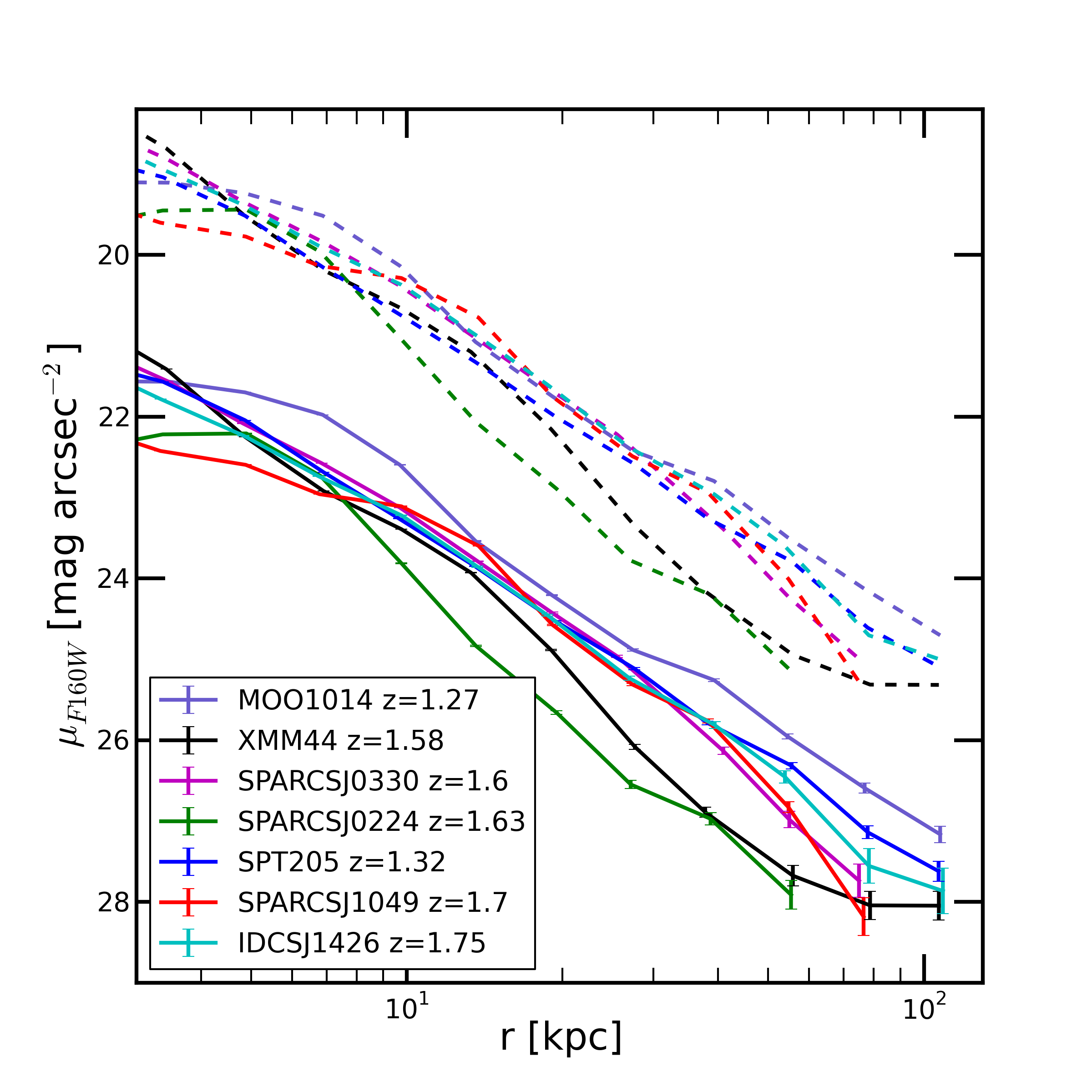
Figure 3: F160W surface brightness profiles out to 100 kpc for the high redshift ($z>1$) clusters. Solid lines are observed profiles and dashed lines represent surface brightness profiles that have e+k and cosmological dimming corrections applied. The e+k corrections are derived from a BC03 SSP model with Chabrier IMF, $z_{f}=3$, and solar metallicity. Surface brightness profiles are terminated when the uncertainty reaches $>0.3$ mag arcsec^-2.

4 Results

4.1 The M_⋆ $-$ M_500,c Relation

We convert from the observed luminosities of the BCG+ICL to stellar masses by applying a mass-to-light ratio for the same stellar population model as in §3. All photometric data (GZZ05, Paper II, and high-redshift) are converted using the same stellar population synthesis models. In this conversion we do not attempt to account for gradients in M/L. We refer the reader to Paper I for a detailed discussion of metallicity gradients in the BCG+ICL. Age gradients can also induce M/L gradients, but are expected to be small outside the central core of the BCG.

The luminosity and stellar mass in apertures of 10, 50, and 100 kpc are given for the high-redshift sample in Table 4.1. While it would also be of interest to measure these quantities within fixed fractions of r_500,c, we cannot do so because of the restricted radial extent of our data coupled with the large range of r_500,c, which make it difficult to define $r/$r_500,c apertures applicable to the full sample. Values within fixed physical apertures thus provide more robust observable quantities.

In Figure 4 we show the stellar mass of the BCG+ICL within 100 kpc as a function of M_500,c. In Paper II we found that the stellar mass within 100 kpc goes as M_⋆$\propto$M_500,c^α, with $\alpha=0.37\pm 0.05$ for our sample of 23 clusters with $\bar{z}=0.4$ and a range in mass from 3$\times 10^{13}$ $-$ 9$\times 10^{14}$ M_⊙. From Figure 4, we see that the sample of low-redshift clusters (black stars) also lies on this relation, shown in blue. For the high-redshift systems, we find smaller total stellar masses within 100 kpc at a given M_500,cfor clusters more massive than $10^{14}M_{\odot}$.

The IllustrisTNG simulations provide an interesting point of comparison. We overplot in Figure 4 the M_⋆$-$M_500,c relation derived by Pillepich et al. (2018) at $r<100$ kpc for IllustrisTNG. Those authors commented that at $r<30$ kpc the slope derived from the simulations was too steep compared to the data from Kravtsov et al. (2014), but had a similar normalization at M_500,c$=10^{14}M_{\odot}$. We find a similar result compared to Pillepich et al. (2018), but now for data extending to $r\sim 100$ kpc. The slope from the simulations is somewhat steeper ($\alpha=0.59$) than the slope from our Paper II, but the normalization at M_500,c$=10^{14}$ kpc is similar. As noted in Pillepich et al. (2018), a similar mismatch at the highest masses is seen in other simulations (e.g. Ragone-Figueroa et al., 2013; Hahn et al., 2017; Bahé et al., 2017).

In Figure 5 we show the same clusters, but now excluding the inner 10 kpc from the mass measurements, as the stellar mass is dominated by the central BCG at these radii. We perform an orthogonal distance regression fit to the intermediate redshift data with the relation

$$\log\textrm{M}_{\star}=\alpha\log\left(\frac{M_{500,c}}{2\times 10^{14}M_{\odot}}\right)+\beta.$$ (1)

In this equation the normalization of the relation, $\beta$, is the log of the stellar mass at $10<r<100$ kpc for a cluster with M_500,c$=$2$\times 10^{14}$ M_⊙. For $10<r<100$ kpc, the $\log\leavevmode\nobreak\$M_⋆ $-\leavevmode\nobreak\ \log\leavevmode\nobreak\$M_500,c relation for the intermediate sample has a slightly steeper slope, $\alpha=0.48\pm 0.06$, than when the central 10 kpc are included. This fit is derived excluding the cluster CL J1226+3332 at $z=0.89$. CL J1226+3332 is the only cluster in any of the subsamples that lies between $z=0.6$ and $z=1.2$. By excluding it we narrow the redshift window over which the intermediate-redshift relation is determined.

The data for the high-redshift sample are consistent with having the same slope, but the large uncertainties and limited number of low-mass clusters preclude a meaningful, independent determination of the slope for this sample. We therefore in the next section assume a redshift-independent slope of $\alpha=0.48$ and focus upon constraining evolution in the normalization $\beta$.

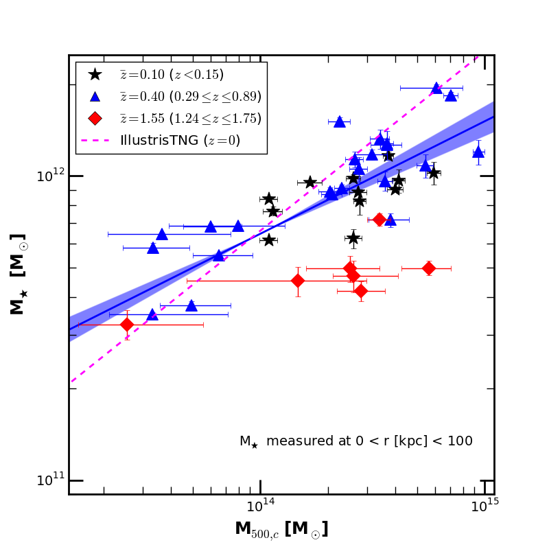
Figure 4: BCG+ICL stellar mass at $r<100$ kpc as a function of M_500,c for the complete sample. Black stars are systems from GZZ13 with $z<0.15$, blue triangles are from Paper II (intermediate-redshift sample), and red diamonds represent the high-redshift cluster sample. The solid blue line represents the best-fit relation to the BCG+ICL content within 100 kpc of the intermediate redshift sample with log(M_⋆/M_⊙)$=(0.37\pm 0.05)$log(M_500,c/2$\times 10^{14}$M_⊙)$+(11.92\pm 0.02)$, with the shaded region corresponding to the 1$\sigma$ confidence region for the relation. The low-redshift sample of GZZ13 falls near this relation while the high-redshift sample on average exhibits lower BCG+ICL  stellar masses at M_500,c$>10^{14}M_{\odot}$. For comparison, we also show the $z=0$ relation derived for the IllustrisTNG simulations by Pillepich et al. (2018), which is slightly steeper than the observed relation but has a similar normalization. All stellar masses are derived at the cluster redshifts assuming passive evolution, with $z_{f}=3$ and solar metallicity, as described in the text.

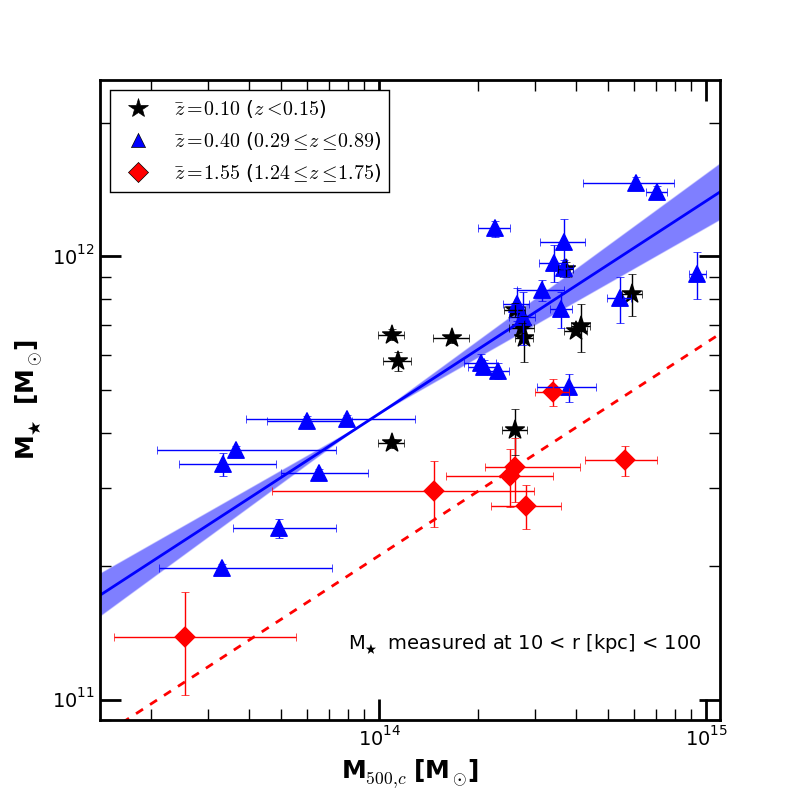
Figure 5: Stellar mass within $10<r<100$ kpc as a function of M_500,c. Markers and colors are as in Figure 4. The solid blue line is the best-fit to the intermediate redshift sample, also as in Figure 4. Excluding the stellar mass in the central 10 kpc produces a steeper relationship with M_500,c, log(M_⋆/M_⊙)$=(0.48\pm 0.06)$log(M_500,c [M_⊙])$+(11.79\pm 0.02$), indicating that the central BCG represents a larger fraction of the total BCG+ICL light inside 100 kpc in groups relative to clusters. The high redshift clusters are consistent with following the same functional relation as at lower redshifts, but shifted to lower M_⋆ by a factor of $2.08\pm 0.21$. The best-fit relation for the high-redshift sample is shown in dashed red, assuming the same slope as for the intermediate redshift sample.

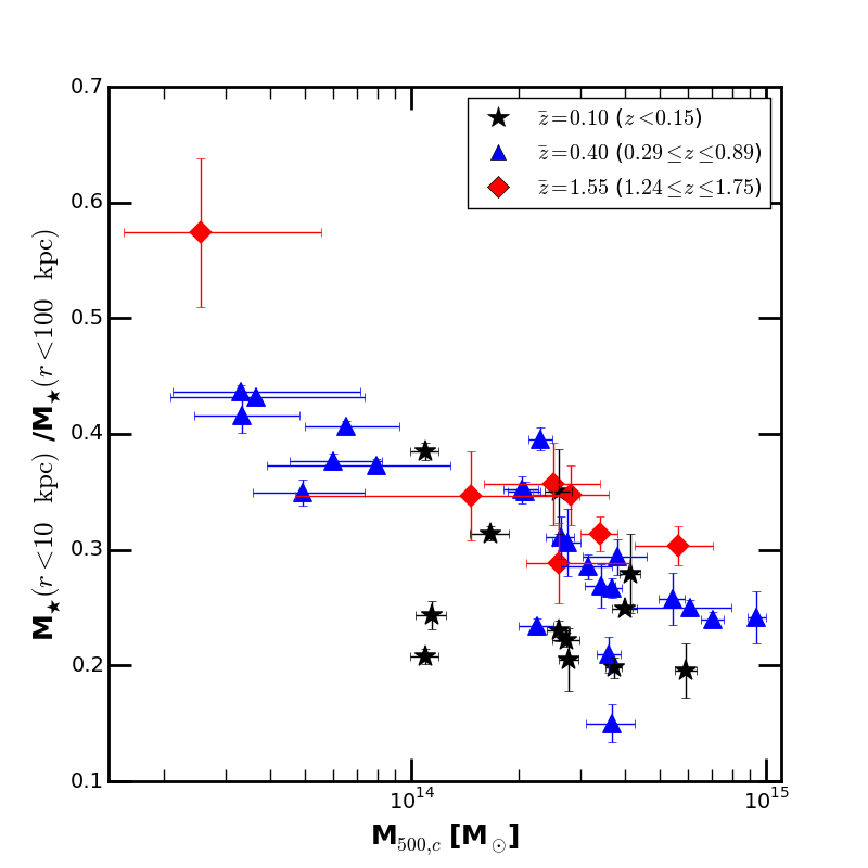
Figure 6: The fraction of the stellar mass within the central 10 kpc relative to the total within 100 kpc, plotted as a function of M_500,c for the complete sample. Systems at all redshifts show a trend of lower central concentration with increasing M_500,c, with no significant shift in this relation betwen samples.

Table 2: Luminosity and Stellar Mass for High-redshift Sample

• Stellar masses are derived using the stellar population model described in section 4.1. Quoted uncertainties on the stellar mass do not reflect systematic errors associated with the mass to light conversion, including the choice of IMF and stellar population age and metallicity. These uncertainties also do not account for any gradients in the M/L ratio of the BCG+ICL, as seen in Paper I.

4.2 Evolution in the M_⋆ $-$ M_500,c Relation and BCG+ICL Stellar Mass Growth

On its surface, the coincidence of the low and intermediate redshift points in Figures 4 and 5 suggests little to no evolution in the BCG+ICL since $\bar{z}=0.4$. However, semi-analytic models and numerical simulations typically predict substantial late-time growth of the ICL. For example, the semi-analytic models of Contini et al. (2014); Contini et al. (2018), which are based upon the Millennium simulations, predict that the ICL has doubled in stellar mass since $z=0.5$. Several recent observational studies concur, suggesting that this growth is driven by the addition of stars from mergers and stripping events (Burke et al., 2012; Zhang et al., 2016). In contrast, the lack of evolution we observe between the local and intermediate-redshift M_⋆ $-$ M_500,c relations in Figures 4 and 5 suggests that late M_⋆ growth within $100$ kpc is modest.

One way out of this conclusion is to posit that M_⋆ growth is matched by growth in M_500,c so that clusters evolve along the M_⋆ $-$ M_500,c relation. However, the expected modest mass growth in M_500,c, $\sim$20% from $z=0.4$ to $z=0.1$, limits the M_⋆ growth in this scenario to $<$ 10%. Therefore, reconciliation with the theoretical expectation is only possible if any substantial late time ICL growth occurs at $r>100$ kpc, a radial regime that is not constrained by our data.

Although there is little if any evolution in the normalization $\beta$ of the relation from $\bar{z}=0.4$ to $\bar{z}=0.1$, there is evolution prior to $\bar{z}=0.4$. To quantify that evolution, we fit each of our three redshift sub-samples with equation 1 using a fixed slope of $\alpha=0.48$, as found for the intermediate-redshift sample at $10<r<100$ kpc. For the intermediate-redshift sample, we again exclude the cluster CL J1226+3332 from the fit.

We present our $\beta$ values for each redshift bin in Table 3. As expected from Figure 5, we see that the low-redshift and intermediate-redshift samples have statistically consistent normalization ($\beta=11.77\pm 0.03$ and $\beta=11.79\pm 0.02$, respectively). For the high-redshift sample, the normalization is significantly different ($\beta=11.47\pm 0.04$). Thus, between the high-redshift ($\bar{z}=1.55$) and intermediate-redshift ($\bar{z}=0.4$) samples, the normalization of the M_⋆$-$M_500,c relation evolves by a factor of $2.08\pm 0.21$ ($\Delta\beta=0.32\pm 0.06$) for M_⋆ measured within $10<r<100$ kpc. At lower redshift, any growth in the BCG+ICL stellar mass within $10<r<100$ kpc must correspond to evolution along the observed M_⋆$-$M_500,c relation.

Our results indicate that the epoch between the high- and intermediate-redshift samples ($z\simeq 0.6-1.2$) is a key period for BCG+ICL development within 100 kpc. The observed lack of evolution in the M_⋆$-$M_500,c relation at low-redshift is correctly predicted by Pillepich et al. (2018). These authors find no evolution in IllustrisTNG since $z=1$, which coupled with our data suggests that the bulk of the evolution may occur rapidly just before this epoch. It is important for future studies to add clusters at $z\sim 1$ to bridge the gap between our intermediate- and high-redshift samples and thus better map the redshift evolution of this relation.

Table 3: M_⋆-M_500,c Normalization ($\beta$) of the M_⋆-M_500,c Relation

$\bar{z}$	$z$ range	$\;\;\;\;\;\;\;\;\beta$
0.10	[0.0578,0.1237]	$11.77\pm 0.03$
0.40	[0.288,0.57]	$11.79\pm 0.02$
1.55	[1.24,1.75]	$11.47\pm 0.04$

• Normalization ($\beta$) of the best-fit M_⋆-M_500,c relation for all redshift bins with an assumed slope equal to that of best-fit to the intermediate redshift sample. The high-redshift sample shows a lower $\beta$ compared to the samples the lower redshift samples, which have the same $\beta$ within uncertainties. The data thus imply that there is a transition from rapid BCG+ICL growth at $10<r<100$ kpc at early times to minimal growth at these radii subsequently.

4.3 Growth of the BCG+ICL in a Typical Cluster

We are not directly observing an evolutionary sequence between epochs, but rather measuring M_⋆  over a similar range in M_500,c at three epochs. To constrain the growth of the BCG+ICL, we must adopt the results from models of structure formation that describe how clusters grow in mass between the three epochs.

For a Tinker et al. (2008) mass function, evolution of the cluster mass function results in an increase in M_500,c of roughly a factor of 4-5 from $z=1.5$, which is approximately the mean redshift of our high-redshift sample, to $z=0$. For example, a galaxy group with M_500,c=5$\times 10^{13}$ M_⊙ at $z=1.5$ will grow to M_500,c$\simeq$ 2$\times 10^{14}$ M_⊙ by $z=0$ (e.g. hmfcalc.org, Murray et al., 2013).

One might naïvely expect similar growth in M_⋆. However, as emphasized by Diemer et al. (2013a, b), this increase in M_500,c is not all due to true physical growth of the cluster. Rather, much of the increase is due to pseudo-evolution arising from the definition of M_500,c relative to the critical density ($\rho_{c}$). As $\rho_{c}$ decreases with time, the radius within which M_500,c is measured increases, leading to a corresponding increase in M_500,c. After correcting for this pseudo-evolution via the approach in Diemer et al. (2013a), the growth for a cluster with M_500,c=5$\times 10^{13}$ M_⊙ at $z=1.5$ is only a factor of 1.4 from $z=1.5$ to $z=0$.

Keeping this factor in mind, we now consider the inferred stellar mass growth for this cluster, using the observed M_⋆$-$ M_500,c relation. If the M_⋆ $-$ M_500,c relation does not evolve, then the factor of four growth in M_500,c corresponds to a factor of 1.9 ($4^{\alpha}$ for $\alpha=0.48$) growth in M_⋆, the stellar mass content at $10<r<100$ kpc. Including evolution of the normalization $\beta$ with redshift, we find that at $10<r<100$ kpc the stellar mass of the BCG+ICL grows by a factor of 3.8 – 1.9$\times$ from mass growth along the sequence and $2\times$ associated with the increase in $\beta$. The bulk of this growth occurs during the epoch between the high- and intermediate-redshift samples. It is during this epoch when we see $\beta$ evolve, and when M_500,c is increasing most rapidly.

We now place these results within the context of previous measurements. The level of evolution in the ICL content here—a factor of $\sim 3.8$ since $\bar{z}=1.55$—is similar to the factor of $2-4$ increase in the BCG+ICL light at $\mu_{J}>22$ mag arcsec^-2, within r_500,c, and since $z=1$ measured by Burke et al. (2012). This amount of growth is also consistent with observed evolution in stellar mass density profiles (see Figure 7 of van der Burg et al., 2015). It is, however, lower than the growth of 90% since $z=1$ predicted by Contini et al. (2014); Contini et al. (2018). As we discussed previously, this contradiction can be resolved by invoking significant growth at radii beyond 100 kpc. We infer that with our data we are witnessing substantial growth of the BCG+ICL at $r<100$ kpc between $\bar{z}=1.55$ and 0.4. At lower redshifts, any growth must occur outside of our observational aperture. It is important that simulations address the radii at which growth is occurring as a function of redshift.

4.4 Evolution of the BCG+ICL Spatial Distribution

While we cannot probe the evolution of the BCG+ICL beyond 100 kpc, we can investigate whether we see evidence of inside-out growth over the radial range of our data. Specifically, we now consider whether there is relative evolution between the inner 10 kpc and the annulus at $10<r<100$ kpc. Figure 6 shows the fraction of the total stellar mass within 100 kpc that lies within the central 10 kpc. There is no statistically significant evolution in this relation between the high-redshift sample and the intermediate- and low-redshift samples. We also obtain similar results for larger central apertures (e.g. 20 kpc).

We conclude that at fixed cluster mass, the concentration of the stellar mass is constant across redshift. However, since any individual cluster will continue to gain mass over time, this conclusion does not mean that concentration of stellar mass for a single cluster stays fixed. Rather, as a cluster grows, we expect its stellar mass concentration to evolve along the relation shown in Figure 6. For a given cluster the BCG+ICL will become less concentrated over time, and a higher proportion of stellar mass that lies outside the central 10 kpc. This accretion of stars with ever-larger orbits in the dark matter potential is inside-out growth.

The paradigm of inside-out growth has previously been invoked for massive ellipticals. Compact, dense stellar cores form very early ($z>2$) and subsequent stellar mass growth occurs at larger radii (van Dokkum et al., 2010; Patel et al., 2013; van der Burg et al., 2014; Bai et al., 2014; Hill et al., 2017; van de Sande et al., 2013). The BCG+ICL constitutes the extreme mass end of the elliptical population, and it is therefore natural to expect similar properties and stellar mass growth histories. Patel et al. (2013) found that 50% of the light within 100 kpc of massive galaxies at $z\sim 1.5$ is contained outside of 10 kpc (see also Hill et al. 2017 for similar conclusions), similar to the fraction that we observe for the BCG+ICL in the lowest mass groups here (Figure 6). Our findings quantify this growth for the BCG+ICL and are not qualitatively different than what one would have expected given our understanding of the growth of massive ellipticals.

5 Conclusions

By combining three samples of galaxy groups and clusters spanning a wide range in redshift ($0.03<z<1.75$) and mass (M_500,c$=2.5$$\times 10^{13}$$-$8$\times 10^{14}$ M_⊙), we measure the growth of the stellar mass of the BCG+ICL, M_⋆, within $10<r<100$ kpc over the last ten Gyr. In particular:

1. We derive a best-fit relation between M_⋆ at $10<r<100$ kpc and M_500,c  of the form log(M_⋆/M_⊙)$=\alpha$log(M_500,c/2$\times 10^{14}$M_⊙)$+\beta$ for our intermediate-redshift sample ($\bar{z}=0.4$) – the sample for which we have the best data. We find a slope $\alpha=0.48\pm 0.06$ and a normalization $\beta=11.79\pm 0.02$. The slope of this relation is steeper than that obtained for $r<100$ kpc in Paper II ($\alpha=0.37\pm 0.05$). The difference comes from excluding here the inner 10 kpc, where the BCG dominates the stellar mass.

2. Fixing the slope to $\alpha=0.48$ for our other redshift samples, we quantify how the normalization, $\beta$, of the M_⋆$-$M_500,c relation evolves. For a cluster with M_500,c$=$ 2$\times 10^{14}$ M_⊙, the BCG+ICL stellar mass within $10<r<100$ kpc is given by $\beta=11.77\pm 0.03$ for the low-redshift sample ($\bar{z}=0.10$), $11.79\pm 0.02$ for the intermediate-redshift sample ($\bar{z}=0.40$), and $11.47\pm 0.04$ for the high-redshift sample ($\bar{z}=1.55$). There is a factor of $2.08\pm 0.21$ increase in the stellar mass between the high- and intermediate-redshift samples at a fixed M_500,c.

3. We consider the overall increase in M_⋆ for a typical cluster since $z=1.5$ using the observed M_⋆$-$M_500,c relations in conjunction with theoretical predictions for the evolution of the halo mass function. For a cluster with M_500,c$\simeq$ 2$\times 10^{14}$ M_⊙ at $z=0$, the BCG+ICL stellar mass within $10<r<100$ kpc with increases by a factor of $\sim 3.8$ since $z=1.5$. This growth in the BCG+ICL stellar mass exceeds the physical mass increase of the cluster, which is only a factor of 1.4 after correcting for the pseudo-evolution of M_500,c arising from the changing critical density $\rho_{c}$.

4. We find evidence for inside-out mass growth of the BCG+ICL at $r<100$ kpc over the past ten Gyrs. We characterize the spatial concentration of the BCG+ICL using the ratio of the BCG+ICL stellar mass within 10 kpc to the total BCG+ICL stellar mass within 100 kpc. We observe an anti-correlation between the BCG+ICL concentration and M_500,c that is independent of redshift. Consequently, as a cluster grows in M_500,c, it must preferentially gain stellar mass at $r>10$ kpc to remain on the observed relation.

We interpret the above results in terms of inside-out growth of the BCG+ICL that eventually progresses to radii beyond those encompassed in our measurement aperture. We directly observe that the BCG+ICL  gains stellar mass at 10 to 100 kpc more rapidly than within the central 10 kpc. At early times, the stellar halo at $10<r<100$ kpc forms more rapidly than the physical mass growth of the cluster, as evidenced by the evolution of the normalization in the M_⋆$-$M_500,c relation. At later times (since $\bar{z}=0.4$), there is little stellar mass growth at these radii. Our observational constraints thus require that continued BCG+ICL growth must occur at even larger radii if theoretical models predicting significant late-time growth are correct. Tracing the evolution of the BCG+ICL, especially beyond $\sim$100 kpc, should be a priority for simulators, as future facilities such as Euclid and WFIRST will be able to measure the BCG+ICL growth at those radii.

Acknowledgements

We thank the referee, Emanuele Contini, for his careful review of this paper. We also thank Adam Muzzin for his helpful comments, and Kyle Finner and James Jee for providing a lensing mass for SpARCS J1049. We acknowledge support from the National Science Foundation through grant NSF-1108957. Support for Program numbers 12634 and 12575 was provided by NASA through a grant from the Space Telescope Science Institute, which is operated by the Association of Universities for Research in Astronomy, Incorporated, under NASA contract NAS5-26555. AIZ acknowledges support from NSF grant AST-0908280 and NASA grant ADP-NNX10AD47G. The archival and Guest Observer data are based on observations made with the NASA/ESA Hubble Space Telescope, which is operated by the Space Telescope Science Institute.

References

- Bahé et al. (2017) Bahé Y. M., et al., 2017, MNRAS, 470, 4186
- Bai et al. (2014) Bai L., et al., 2014, ApJ, 789, 134
- Bellstedt et al. (2016) Bellstedt S., et al., 2016, MNRAS, 460, 2862
- Bertin & Arnouts (1996) Bertin E., Arnouts S., 1996, A&AS, 117, 393
- Brodwin et al. (2015) Brodwin M., et al., 2015, ApJ, 806, 26
- Brodwin et al. (2016) Brodwin M., McDonald M., Gonzalez A. H., Stanford S. A., Eisenhardt P. R., Stern D., Zeimann G. R., 2016, ApJ, 817, 122
- Bruzual & Charlot (2003) Bruzual G., Charlot S., 2003, MNRAS, 344, 1000
- Burke et al. (2000) Burke D. J., Collins C. A., Mann R. G., 2000, ApJ, 532, L105
- Burke et al. (2012) Burke C., Collins C. A., Stott J. P., Hilton M., 2012, MNRAS, 425, 2058
- Chabrier (2003) Chabrier G., 2003, PASP, 115, 763
- Chiu et al. (2016) Chiu I., et al., 2016, MNRAS, 455, 258
- Collins et al. (2009) Collins C. A., et al., 2009, Nature, 458, 603
- Contini et al. (2014) Contini E., De Lucia G., Villalobos Á., Borgani S., 2014, MNRAS, 437, 3787
- Contini et al. (2018) Contini E., Yi S. K., Kang X., 2018, MNRAS, 479, 932
- De Lucia & Blaizot (2007) De Lucia G., Blaizot J., 2007, MNRAS, 375, 2
- DeMaio et al. (2015) DeMaio T., Gonzalez A. H., Zabludoff A., Zaritsky D., Bradač M., 2015, MNRAS, 448, 1162
- DeMaio et al. (2018) DeMaio T., Gonzalez A. H., Zabludoff A., Zaritsky D., Connor T., Donahue M., Mulchaey J. S., 2018, MNRAS, 474, 3009
- Diemer (2015) Diemer B., 2015, Colossus: COsmology, haLO, and large-Scale StrUcture toolS, Astrophysics Source Code Library (ascl:1501.016)
- Diemer et al. (2013a) Diemer B., More S., Kravtsov A. V., 2013a, ApJ, 766, 25
- Diemer et al. (2013b) Diemer B., Kravtsov A. V., More S., 2013b, ApJ, 779, 159
- Donahue et al. (2014) Donahue M., et al., 2014, ApJ, 794, 136
- Donahue et al. (2016) Donahue M., et al., 2016, ApJ, 819, 36
- Duffy et al. (2008) Duffy A. R., Schaye J., Kay S. T., Dalla Vecchia C., 2008, MNRAS, 390, L64
- Fassbender et al. (2014) Fassbender R., et al., 2014, A&A, 568, A5
- Gonzalez et al. (2005) Gonzalez A. H., Zabludoff A. I., Zaritsky D., 2005, ApJ, 618, 195
- Gonzalez et al. (2013) Gonzalez A. H., Sivanandam S., Zabludoff A. I., Zaritsky D., 2013, ApJ, 778, 14
- Hahn et al. (2017) Hahn O., Martizzi D., Wu H.-Y., Evrard A. E., Teyssier R., Wechsler R. H., 2017, MNRAS, 470, 166
- Hill et al. (2017) Hill A. R., et al., 2017, ApJ, 837, 147
- Hinshaw et al. (2013) Hinshaw G., et al., 2013, ApJS, 208, 19
- Jordi et al. (2006) Jordi K., Grebel E. K., Ammon K., 2006, A&A, 460, 339
- Ko & Jee (2018) Ko J., Jee M. J., 2018, ApJ, 862, 95
- Kravtsov et al. (2014) Kravtsov A., Vikhlinin A., Meshscheryakov A., 2014, preprint, (arXiv:1401.7329)
- Lidman et al. (2012) Lidman C., et al., 2012, MNRAS, 427, 550
- Lin et al. (2013) Lin Y.-T., Brodwin M., Gonzalez A. H., Bode P., Eisenhardt P. R. M., Stanford S. A., Vikhlinin A., 2013, ApJ, 771, 61
- Mahdavi et al. (2013) Mahdavi A., Hoekstra H., Bildfell C., Jeltema T., Henry J. P., 2013, ApJ, 767, 116
- Mo et al. (2016) Mo W., et al., 2016, ApJ, 818, L25
- Murray et al. (2013) Murray S. G., Power C., Robotham A. S. G., 2013, Astronomy and Computing, 3, 23
- Nantais et al. (2016) Nantais J. B., et al., 2016, A&A, 592, A161
- Navarro et al. (1997) Navarro J. F., Frenk C. S., White S. D. M., 1997, ApJ, 490, 493
- Oemler (1976) Oemler A. J., 1976, ApJ, 209, 693
- Patel et al. (2013) Patel S. G., et al., 2013, ApJ, 766, 15
- Pillepich et al. (2018) Pillepich A., et al., 2018, MNRAS, 475, 648
- Postman et al. (2012) Postman M., et al., 2012, ApJS, 199, 25
- Ragone-Figueroa et al. (2013) Ragone-Figueroa C., Granato G. L., Murante G., Borgani S., Cui W., 2013, MNRAS, 436, 1750
- Schellenberger et al. (2015) Schellenberger G., Reiprich T. H., Lovisari L., Nevalainen J., David L., 2015, A&A, 575, A30
- Schombert (1988) Schombert J. M., 1988, ApJ, 328, 475
- Stott et al. (2010) Stott J. P., et al., 2010, ApJ, 718, 23
- Tinker et al. (2008) Tinker J., Kravtsov A. V., Klypin A., Abazajian K., Warren M., Yepes G., Gottlöber S., Holz D. E., 2008, ApJ, 688, 709
- Tozzi et al. (2015) Tozzi P., et al., 2015, ApJ, 799, 93
- Vikhlinin et al. (2009) Vikhlinin A., et al., 2009, ApJ, 692, 1033
- Webb et al. (2015) Webb T. M. A., et al., 2015, ApJ, 814, 96
- Whiley et al. (2008) Whiley I. M., et al., 2008, MNRAS, 387, 1253
- Zhang et al. (2016) Zhang Y., et al., 2016, ApJ, 816, 98
- Zhang et al. (2019) Zhang Y., et al., 2019, ApJ, 874, 165
- Zibetti et al. (2005) Zibetti S., White S. D. M., Schneider D. P., Brinkmann J., 2005, MNRAS, 358, 949
- van Dokkum et al. (2010) van Dokkum P. G., et al., 2010, ApJ, 709, 1018
- van de Sande et al. (2013) van de Sande J., et al., 2013, ApJ, 771, 85
- van der Burg et al. (2014) van der Burg R. F. J., Muzzin A., Hoekstra H., Wilson G., Lidman C., Yee H. K. C., 2014, A&A, 561, A79
- van der Burg et al. (2015) van der Burg R. F. J., Hoekstra H., Muzzin A., Sifón C., Balogh M. L., McGee S. L., 2015, A&A, 577, A19