Predicting critical ignition in slow-fast excitable models

Abstract

Linearization around unstable travelling waves in excitable systems can be used to approximate strength-extent curves in the problem of initiation of excitation waves for a family of spatially confined perturbations to the rest state. This theory relies on the knowledge of the unstable travelling wave solution as well as the leading left and right eigenfunctions of its linearization. We investigate the asymptotics of these ingredients, and utility of the resulting approximations of the strength-extent curves, in the slow-fast limit in two-component excitable systems of FitzHugh-Nagumo type, and test those on four illustrative models. Of these, two are with degenerate dependence of the fast kinetic on the slow variable, a feature which is motivated by a particular model found in the literature. In both cases, the unstable travelling wave solution converges to a stationary “critical nucleus” of the corresponding one-component fast subsystem. We observe that in the full system, the asymptotics of the left and right eigenspaces are distinct. In particular, the slow component of the left eigenfunction corresponding to the translational symmetry does not become negligible in the asymptotic limit. This has a significant detrimental effect on the critical curve predictions. The theory as formulated previously uses an heuristic to address a difficulty related to the translational invariance. We describe two alternatives to that heuristic, which do not use the misbehaving eigenfunction component. These new heuristics show much better predictive properties, including in the asymptotic limit, in all four examples.

I Introduction

Excitable systems represent a distinct modeling legacy in the context of biological systems, especially regarding cardiac and neuronal cells. These models utilize the existence of a typically state-dependent threshold to distinguish between relaxation and transiently amplified dynamics. In classic FitzHugh-Nagumo type models this threshold is explicitly the unstable branch of the fast variable nullcline, volumes have been dedicated to investigations around the response of excitable models to driving.

In the nomenclature of previous efforts Bezekci-etal-2015 , we focus the formalism of a “stimulation by voltage”, which corresponds to an initial value problem for reaction diffusion models of the form,

$$\partial_{t}{\mathbf{u}}={\mathbf{D}}\partial^{2}_{x}{\mathbf{u}}+{\Gamma}{\mathbf{f}}({\mathbf{u}}),$$ (2)

for a two-component field, ${\mathbf{u}}=[{u_{1}},{u_{2}}]$. We assume that the model is non-dimensionalized with respect to the dynamic variables ${u_{1}}$, ${u_{2}}$, as well as the independent variables ${x}$ and ${t}$. We restrict ourselves to the models where only the first component is diffusive, so ${\mathbf{D}}=\mathrm{diag}\left(1,0\right)$. The time-scale separation of the dynamics of ${u_{1}}$ and ${u_{2}}$ is controlled by parameter ${\gamma}$, with the time-scale of ${u_{1}}$ considered fixed, so ${\Gamma}=\mathrm{diag}(1,{\gamma})$. Further, we assume that ${\mathbf{f}}({\bar{{\mathbf{u}}}})=\mathbf{0}$ for a unique, asymptotically stable rest-state ${\bar{{\mathbf{u}}}}$. The limit ${\gamma}\to 0$ designates the transition from moving solutions (${\gamma}>0$, ${c}\neq 0$) to stationary solutions (${\gamma}=0$, ${c}=0$) of (2). In this work we concern ourselves primarily with the transient dynamics in the vicinity of the traveling wave solutions of these slow-fast systems.

Traveling wave solutions of (2) satisfy a nonlinear eigenvalue problem posed on the real line ${x}\in\mathbb{R}$,

$$\mathbf{0}={\mathbf{D}}\partial^{2}_{x}{\tilde{{\mathbf{u}}}}+{\tilde{{c}}}\partial_{x}{\tilde{{\mathbf{u}}}}+{\mathbf{f}}({\tilde{{\mathbf{u}}}}),$$ (3)

for the wave solution ${\tilde{{\mathbf{u}}}}$ and the associated wave speed ${\tilde{{c}}}\neq 0$. Additionally, we require that the wave approach the rest state asymptotically, ${\tilde{{\mathbf{u}}}}({x}\to\pm\infty)\to{\bar{{\mathbf{u}}}}$ so that the solution is localized in space, and a homoclinic connection to and from the rest state in the co-moving frame. The simplest solutions to (3) are two single-pulse waves: a faster, stable wave ${\check{{\mathbf{u}}}}$, and the slower, unstable wave ${\hat{{\mathbf{u}}}}$, with $|{\hat{{c}}}|<|{\check{{c}}}|$. When speaking about general solutions of (3), we shall refer to generic waves ${\tilde{{\mathbf{u}}}}$ and associated generic speeds ${\tilde{{c}}}$.

The linear stability of these waves is determined by the eigenspectrum $({\sigma_{{i}}},{\mathbf{v}_{{i}}})$ of the operator ${\mathcal{L}}$, the linearization about (3),

$${\mathcal{L}}={\mathbf{D}}\partial^{2}_{x}+{\tilde{{c}}}\partial_{x}+{{\mathbf{f}}^{\prime}}({\tilde{{\mathbf{u}}}}),$$ (4)

which is guaranteed to have a marginal eigenfunction, ${\mathcal{L}}{\mathbf{v}}=0{\mathbf{v}}$, where ${\mathbf{v}}=\partial_{x}{\tilde{{\mathbf{u}}}}$, due to the translational symmetry. Further, for the unstable asymptotic wave solution ${\hat{{\mathbf{u}}}}$, the operator ${\mathcal{L}}$ must have exactly one unstable mode, ${\sigma}>0$, whose shape describes the fastest-growing mode in the co-moving frame. We enumerate the modes in the decreasing order of the real parts, so for the unstable wave,

$${\sigma_{1}}>{\sigma_{2}}=0>\mathrm{Re}\left({\sigma_{3}}\right)\geq\dots.$$

Similarly, the inner-product over the domain,

$$\left\langle\leavevmode\hbox{$\displaystyle{{\mathbf{w}}}$}\phantom{\makebox[0.0pt][l]{\leavevmode\hbox{$\displaystyle{{\mathbf{w}}}$}\leavevmode\hbox{$\displaystyle{{\mathcal{L}}{\mathbf{v}}}$}}}\,\right|\left.\phantom{\makebox[0.0pt][l]{\leavevmode\hbox{$\displaystyle{{\mathbf{w}}}$}\leavevmode\hbox{$\displaystyle{{\mathcal{L}}{\mathbf{v}}}$}}}\leavevmode\hbox{$\displaystyle{{\mathcal{L}}{\mathbf{v}}}$}\right\rangle=\int\limits_{-\infty}^{\infty}{\mathbf{w}}^{\dagger}{\mathcal{L}}{\mathbf{v}}\,\ \mathrm{d}{x},$$

defines the set of adjoint eigenfunctions ${\mathbf{w}_{{j}}}$ with eigenvalues $\overline{{\sigma_{{j}}}}$ satisfying the biorthogonality condition $({\sigma_{{j}}}-{\sigma_{{i}}})\left\langle\leavevmode\hbox{$\displaystyle{{\mathbf{w}_{{j}}}}$}\phantom{\makebox[0.0pt][l]{\leavevmode\hbox{$\displaystyle{{\mathbf{w}_{{j}}}}$}\leavevmode\hbox{$\displaystyle{{\mathbf{v}_{{i}}}}$}}}\,\right|\left.\phantom{\makebox[0.0pt][l]{\leavevmode\hbox{$\displaystyle{{\mathbf{w}_{{j}}}}$}\leavevmode\hbox{$\displaystyle{{\mathbf{v}_{{i}}}}$}}}\leavevmode\hbox{$\displaystyle{{\mathbf{v}_{{i}}}}$}\right\rangle=({\sigma_{{j}}}-{\sigma_{{i}}})\delta_{{i}{j}}$. Equivalently, we may consider the right eigenfunctions of the adjoint linear operator, ${{\mathcal{L}}^{\dagger}}$,

$${{\mathcal{L}}^{\dagger}}({\mathbf{u}}){\mathbf{w}}={\mathbf{D}}^{\top}\partial^{2}_{x}{\mathbf{w}}-{\tilde{{c}}}\partial_{x}{\mathbf{w}}+\left[{{\mathbf{f}}^{\prime}}({\tilde{{\mathbf{u}}}})\right]^{\top}{\mathbf{w}},$$

where $(\cdot)^{\top}$ stands for transposed and $(\cdot)^{\dagger}$ for Hermitian conjugate.

The transient dynamics in the vicinity of the unstable solution ${\hat{{\mathbf{u}}}}$ is important phenomenologically for understanding the initiation of e.g., electrical waves in heart tissue. Ref. Bezekci-etal-2015 used the properties of the unstable wave to predict the minimal perturbations to the rest state which lead to the generation of new excitation waves, using a particular notion of ‘smallness’ for the constructed perturbations which relies on assumptions about the behavior of the solution ${\hat{{\mathbf{u}}}}$ and its linearization in the limit ${\gamma}\to 0$. In this work, we investigate the limitations of those assumptions, and test alternative methods for constructing those minimal perturbations. We find that in several cases, the applicability of the existing theory to traveling wave solutions of simple slow-fast models predicts at the very least sub-optimal or occasionally unrealistically large minimal perturbations. We have in mind three specific examples of the models: the classical FitzHugh-Nagumo model in the original formulation FitzHugh-1961 (FHN), the two-variable Karma 1994 model Karma-1994 (Karma) and two-variable reduction of the Fenton-Karma model due to Mitchell and Schaeffer Mitchell-Schaeffer-2003 (MS). To our surprise we found that Karma model is different from the other two in its asymptotics in ${\gamma}$, which has proved to be due to a specific form of dependence of the fast kinetics ${f_{1}}$ on the slow variable ${u_{2}}$, namely via ${u_{2}}^{M}$, with ${M}>1$, whereas in the resting state ${\bar{u}_{2}}=0$. To illustrate further the specifics of such dependence, we have also considered a variation of the FitzHugh-Nagumo model which also has this feature, that is, ${f_{1}}$ depends on ${u_{2}}^{3}$; we shall call it “FHN with cubic recovery”, or FHNCR for short.

The outline of this paper is as follows. First we review the basics of sub- and super-threshold response for classic excitable models of FitzHugh-Nagumo type, the complication from embedding them in spatially extended media, and how to distinguish sub- and super-threshold excitations in space. Second, we review the essential ingredients of the linear theory of critical excitation, in the context of the asymptotics in the slow-fast time scale separation between the activator and inhibitor subsystems. We show that the approach applied to slow-fast systems relies on misleading assumptions about the asymptotic structure of the leading left and right eigenspaces and particularly the form of the adjoint eigenfunctions. We detail the computation of the slow wave solutions, their eigenspectra, and the solution of transient trajectories by direct numerical simulation. Third, we propose heuristics based on minimization principles which do not rely on the slow mode corresponding to translational symmetry, and which outperform the previously suggested skew-product motivated heuristic. Finally we reinforce this conclusion with numerical examples using several slow-fast systems, and use these results to infer properties of the leading eigenspace and the effect of degenerate nonlinearities on observing other nearby saddle solutions.

II Theory

The mathematical problem is posed in the following way. Given an initial condition ${\mathbf{u}}(0,{x})={\bar{{\mathbf{u}}}}+{\bar{\mathbf{h}}}({x};{{x}_{s}},{U_{s}})$ parameterized by the properties $({{x}_{s}},{U_{s}})$ of the stimulus, i.e. a perturbation to the rest state, determine for which configurations will the initial conditions eventually recruit the entire domain – excite the medium – and for which configurations will it return directly to the rest state. In the language of coherent structures, this corresponds to identifying the boundary of the basin of attraction isolating the stable wave solution from the uniform rest state, and projecting this infinite-dimensional manifold down to the shape-modifying parameter space of $({{x}_{s}},{U_{s}})$. Throughout this work we shall use a parameterized perturbation to the rest state, pert & ¯h(x; x_s, U_s) = U_s¯X(x; x_s),
¯X(x; x_s) = e_1¯X^(x; x_s),
¯X^(x; x_s) = H(x_s/2 - x) H(x+ x_s/2), where ${\mathbf{e}_{1}}=\begin{bmatrix}1,0\end{bmatrix}^{\top}$ and $\mathrm{H}({x})$ is the Heaviside distribution, so that $\left\lVert{\bar{\mathbf{h}}}({x};{{x}_{s}},{U_{s}})\right\rVert_{\infty}\equiv{U_{s}}$ and $\left\lVert{\bar{\mathbf{h}}}({x};{{x}_{s}},{U_{s}})\right\rVert_{1}\equiv{{x}_{s}}{U_{s}}$. The choice of ${\mathbf{e}_{1}}=\begin{bmatrix}1,0\end{bmatrix}^{\top}$ means that we restrict consideration exclusively to perturbation of the first component of the system. This is in line with the prospective application of the theory to models of heart or nerve excitability, with the first component representing the transmembrane voltage, and the stimulation effected by external electric fields. Of course, in different application areas, different modalities of the stimulus may be more appropriate.

II.1 Linear theory of critical excitations

Here we present a brief motivation for the linear theory of critical excitations, and recount the assumptions of the method. Given the initial state ${\mathbf{u}}(0,{x})={\hat{{\mathbf{u}}}}({x})+{\hat{\mathbf{h}}}({x})$, where ${\hat{\mathbf{h}}}({x})$ is understood to be perturbatively small, then the dynamics of the state subject to (2) can be understood through the linearization about ${\hat{{\mathbf{u}}}}({\xi})$, with ${\xi}={x}-{\hat{{c}}}{t}-{s}$ the co-moving frame coordinate. The presence of the shift parameter ${s}$ here is due to translational invariance of the problem and its significance and issues associated with its choice are discussed below in Subsection II.2. Expressing the linearized dynamics in terms of the spectral expansion,

$${\mathcal{L}}=\sum_{{k}=1}^{\infty}|\,{\mathbf{v}_{{k}}}\rangle{\sigma_{{k}}}\langle{\mathbf{w}_{{k}}}\,|,$$

$${\tilde{{\mathbf{u}}}}({t},{\xi})={\hat{{\mathbf{u}}}}({\xi})+\sum_{{k}=1}^{\infty}{a_{{k}}}({t}){\mathbf{v}_{{k}}}({\xi}),$$

and recalling that $\mathrm{Re}({\sigma_{1}})>0$, then we can consider the requirement that the sole unstable mode is not excited due to the perturbation,

$$0={a_{1}}({t})=\exp({\sigma_{1}}{t})\left\langle\leavevmode\hbox{$\displaystyle{{\mathbf{w}_{1}}}$}\phantom{\makebox[0.0pt][l]{\leavevmode\hbox{$\displaystyle{{\mathbf{w}_{1}}}$}\leavevmode\hbox{$\displaystyle{{\hat{\mathbf{h}}}({\xi})}$}}}\,\right|\left.\phantom{\makebox[0.0pt][l]{\leavevmode\hbox{$\displaystyle{{\mathbf{w}_{1}}}$}\leavevmode\hbox{$\displaystyle{{\hat{\mathbf{h}}}({\xi})}$}}}\leavevmode\hbox{$\displaystyle{{\hat{\mathbf{h}}}({\xi})}$}\right\rangle,$$ (5)

where we identify the modal amplitudes of the linearization, ${a_{{i}}}(0)=\left\langle\leavevmode\hbox{$\displaystyle{{\mathbf{w}_{{i}}}}$}\phantom{\makebox[0.0pt][l]{\leavevmode\hbox{$\displaystyle{{\mathbf{w}_{{i}}}}$}\leavevmode\hbox{$\displaystyle{{\hat{\mathbf{h}}}({\xi})}$}}}\,\right|\left.\phantom{\makebox[0.0pt][l]{\leavevmode\hbox{$\displaystyle{{\mathbf{w}_{{i}}}}$}\leavevmode\hbox{$\displaystyle{{\hat{\mathbf{h}}}({\xi})}$}}}\leavevmode\hbox{$\displaystyle{{\hat{\mathbf{h}}}({\xi})}$}\right\rangle$. At time ${t}=0$, we express the initial perturbation ${\hat{\mathbf{h}}}$ to the critical solution ${\hat{{\mathbf{u}}}}$ in terms of a perturbation ${\bar{\mathbf{h}}}$ to the rest state ${\bar{{\mathbf{u}}}}$ so that ${\xi}+{s}={x}$,

$${\hat{\mathbf{h}}}({\xi}+{s};{{x}_{s}},{U_{s}})={\bar{\mathbf{h}}}({\xi}+{s};{{x}_{s}},{U_{s}})+{\bar{{\mathbf{u}}}}-{\hat{{\mathbf{u}}}}({\xi}),$$

where the invariance of the rest state with respect to translational symmetry manifests as a freedom in the origin of the rest-state perturbation, the shift parameter ${s}$. The freedom in choosing this origin must be dealt with and the simplest functional method relies on computing the root of a scalar function, whose form is heuristically determined based on assumptions about the asymptotic structure of the eigenfunctions. The combined system is, linsys N_0 &= U_s ⟨$\displaystyle{{\mathbf{K}_{0}}({\xi})}$$\displaystyle{{\mathbf{K}_{0}}({\xi})}$$\displaystyle{{\bar{\mathbf{X}}}({\xi}+{s};{{x}_{s}})}$ —$\displaystyle{{\mathbf{K}_{0}}({\xi})}$$\displaystyle{{\bar{\mathbf{X}}}({\xi}+{s};{{x}_{s}})}$$\displaystyle{{\bar{\mathbf{X}}}({\xi}+{s};{{x}_{s}})}$ ⟩,
N_ℓ = U_s ⟨$\displaystyle{{\mathbf{K}_{{\ell}}}({\xi})}$$\displaystyle{{\mathbf{K}_{{\ell}}}({\xi})}$$\displaystyle{{\bar{\mathbf{X}}}({\xi}+{s};{{x}_{s}})}$ —$\displaystyle{{\mathbf{K}_{{\ell}}}({\xi})}$$\displaystyle{{\bar{\mathbf{X}}}({\xi}+{s};{{x}_{s}})}$$\displaystyle{{\bar{\mathbf{X}}}({\xi}+{s};{{x}_{s}})}$ ⟩, to be solved for ${U_{s}}$ and ${s}$ as a self-consistent system, for each chosen ${{x}_{s}}$, with functional ${\mathbf{K}_{{\ell}}}$ constructed heuristically for ${\ell}=1,2,3$, in the next section.

II.2 Shift selection

Here we describe three heuristic arguments which lead to different forms of ${\mathbf{K}_{{\ell}}}$, resulting in three different values of the shift ${s}$, and ultimately three different predictions for the critical amplitude, ${U_{s}}$, per chosen extent of the perturbation ${{x}_{s}}$.

The first heuristic seeks to minimize the amplitude ${U_{s}}$ chosen across all the possible choices of the shift, ${s}$. Defining ${\bar{\mathbf{X}}}({\xi};{{x}_{s}})$ according to (LABEL:eq:pert), so that ${\bar{\mathbf{X}}}({\xi};{{x}_{s}})$ is normalized in the $L^{\infty}$-norm, rearranging (LABEL:eq:linsys) for the amplitude of the perturbation,

$${U_{s}}=\left\langle\leavevmode\hbox{$\displaystyle{{\mathbf{w}_{1}}({\xi})}$}\phantom{\makebox[0.0pt][l]{\leavevmode\hbox{$\displaystyle{{\mathbf{w}_{1}}({\xi})}$}\leavevmode\hbox{$\displaystyle{{\hat{{\mathbf{u}}}}({\xi})-{\bar{{\mathbf{u}}}}}$}}}\,\right|\left.\phantom{\makebox[0.0pt][l]{\leavevmode\hbox{$\displaystyle{{\mathbf{w}_{1}}({\xi})}$}\leavevmode\hbox{$\displaystyle{{\hat{{\mathbf{u}}}}({\xi})-{\bar{{\mathbf{u}}}}}$}}}\leavevmode\hbox{$\displaystyle{{\hat{{\mathbf{u}}}}({\xi})-{\bar{{\mathbf{u}}}}}$}\right\rangle\big{/}\left\langle\leavevmode\hbox{$\displaystyle{{\mathbf{w}_{1}}({\xi})}$}\phantom{\makebox[0.0pt][l]{\leavevmode\hbox{$\displaystyle{{\mathbf{w}_{1}}({\xi})}$}\leavevmode\hbox{$\displaystyle{{\bar{\mathbf{X}}}({\xi}+{s};{{x}_{s}})}$}}}\,\right|\left.\phantom{\makebox[0.0pt][l]{\leavevmode\hbox{$\displaystyle{{\mathbf{w}_{1}}({\xi})}$}\leavevmode\hbox{$\displaystyle{{\bar{\mathbf{X}}}({\xi}+{s};{{x}_{s}})}$}}}\leavevmode\hbox{$\displaystyle{{\bar{\mathbf{X}}}({\xi}+{s};{{x}_{s}})}$}\right\rangle,$$ (6)

leads to the maximization of the denominator (as the numerator is independent of ${s}$), and the resulting condition,

$$\partial_{s}\left\langle\leavevmode\hbox{$\displaystyle{{\mathbf{w}_{1}}({\xi})}$}\phantom{\makebox[0.0pt][l]{\leavevmode\hbox{$\displaystyle{{\mathbf{w}_{1}}({\xi})}$}\leavevmode\hbox{$\displaystyle{{\bar{\mathbf{X}}}({\xi}+{s};{{x}_{s}})}$}}}\,\right|\left.\phantom{\makebox[0.0pt][l]{\leavevmode\hbox{$\displaystyle{{\mathbf{w}_{1}}({\xi})}$}\leavevmode\hbox{$\displaystyle{{\bar{\mathbf{X}}}({\xi}+{s};{{x}_{s}})}$}}}\leavevmode\hbox{$\displaystyle{{\bar{\mathbf{X}}}({\xi}+{s};{{x}_{s}})}$}\right\rangle=0,$$

with $\partial^{2}_{s}\left\langle\leavevmode\hbox{$\displaystyle{{\mathbf{w}_{1}}({\xi})}$}\phantom{\makebox[0.0pt][l]{\leavevmode\hbox{$\displaystyle{{\mathbf{w}_{1}}({\xi})}$}\leavevmode\hbox{$\displaystyle{{\bar{\mathbf{X}}}({\xi}+{s};{{x}_{s}})}$}}}\,\right|\left.\phantom{\makebox[0.0pt][l]{\leavevmode\hbox{$\displaystyle{{\mathbf{w}_{1}}({\xi})}$}\leavevmode\hbox{$\displaystyle{{\bar{\mathbf{X}}}({\xi}+{s};{{x}_{s}})}$}}}\leavevmode\hbox{$\displaystyle{{\bar{\mathbf{X}}}({\xi}+{s};{{x}_{s}})}$}\right\rangle<0$. Computing the derivative of this function with respect to ${s}$ can be simplified using the definition of the inner product, which yields

$$\left\langle\leavevmode\hbox{$\displaystyle{{\mathbf{w}_{1}}^{\prime}({\xi})}$}\phantom{\makebox[0.0pt][l]{\leavevmode\hbox{$\displaystyle{{\mathbf{w}_{1}}^{\prime}({\xi})}$}\leavevmode\hbox{$\displaystyle{{\bar{\mathbf{X}}}({\xi}+{s};{{x}_{s}})}$}}}\,\right|\left.\phantom{\makebox[0.0pt][l]{\leavevmode\hbox{$\displaystyle{{\mathbf{w}_{1}}^{\prime}({\xi})}$}\leavevmode\hbox{$\displaystyle{{\bar{\mathbf{X}}}({\xi}+{s};{{x}_{s}})}$}}}\leavevmode\hbox{$\displaystyle{{\bar{\mathbf{X}}}({\xi}+{s};{{x}_{s}})}$}\right\rangle=0,$$

so that we must find only the roots of a simple scalar equation, which when combined with (LABEL:eq:linsys) creates an appropriate solvability condition for ${U_{s}}$.

The second heuristic assumes that the limiting feature of the linear theory is the magnitude of the perturbation to the critical wave, ${\hat{\mathbf{h}}}({\xi}+{s};{{x}_{s}},{U_{s}})$, and a minimization of the perturbation norm in the $L^{2}$ sense, with respect to the shift, ensures the dynamics are appropriately linear and chooses the appropriate origin ${s}$. Expressing the perturbation to the wave in terms of the perturbation to the rest state and minimizing with respect to ${s}$,

$$0=\partial_{s}\int\limits_{-\infty}^{\infty}\left({\hat{\mathbf{h}}}({\xi}+{s};{{x}_{s}},{U_{s}})\right)^{2}\,\mathrm{d}{x}$$

subject to $\partial^{2}_{s}\langle\dots\rangle>0$, ultimately leads to the condition

$$0=\left\langle\leavevmode\hbox{$\displaystyle{{\mathbf{v}_{2}}({\xi})}$}\phantom{\makebox[0.0pt][l]{\leavevmode\hbox{$\displaystyle{{\mathbf{v}_{2}}({\xi})}$}\leavevmode\hbox{$\displaystyle{{\bar{\mathbf{h}}}({\xi}+{s};{{x}_{s}},{U_{s}})+{\bar{{\mathbf{u}}}}-{\hat{{\mathbf{u}}}}({\xi})}$}}}\,\right|\left.\phantom{\makebox[0.0pt][l]{\leavevmode\hbox{$\displaystyle{{\mathbf{v}_{2}}({\xi})}$}\leavevmode\hbox{$\displaystyle{{\bar{\mathbf{h}}}({\xi}+{s};{{x}_{s}},{U_{s}})+{\bar{{\mathbf{u}}}}-{\hat{{\mathbf{u}}}}({\xi})}$}}}\leavevmode\hbox{$\displaystyle{{\bar{\mathbf{h}}}({\xi}+{s};{{x}_{s}},{U_{s}})+{\bar{{\mathbf{u}}}}-{\hat{{\mathbf{u}}}}({\xi})}$}\right\rangle.$$

This reaffirms the importance of the Goldstone mode, and as with heuristic $1$, the condition is combined with (LABEL:eq:linsys) to create an appropriate solvability condition for ${U_{s}}$.

The third heuristic requires that ${a_{2}}(0)=0$,

$${a_{2}}(0)=\left\langle\leavevmode\hbox{$\displaystyle{{\mathbf{w}_{2}}({\xi})}$}\phantom{\makebox[0.0pt][l]{\leavevmode\hbox{$\displaystyle{{\mathbf{w}_{2}}({\xi})}$}\leavevmode\hbox{$\displaystyle{{\bar{\mathbf{h}}}({\xi}+{s};{{x}_{s}},{U_{s}})+{\bar{{\mathbf{u}}}}-{\hat{{\mathbf{u}}}}({\xi})}$}}}\,\right|\left.\phantom{\makebox[0.0pt][l]{\leavevmode\hbox{$\displaystyle{{\mathbf{w}_{2}}({\xi})}$}\leavevmode\hbox{$\displaystyle{{\bar{\mathbf{h}}}({\xi}+{s};{{x}_{s}},{U_{s}})+{\bar{{\mathbf{u}}}}-{\hat{{\mathbf{u}}}}({\xi})}$}}}\leavevmode\hbox{$\displaystyle{{\bar{\mathbf{h}}}({\xi}+{s};{{x}_{s}},{U_{s}})+{\bar{{\mathbf{u}}}}-{\hat{{\mathbf{u}}}}({\xi})}$}\right\rangle,$$

following the same formulation as (5), and is equivalent to the form used in Ref. Bezekci-etal-2015 . As with heuristic $2$, the condition is then combined with (LABEL:eq:linsys) to create an appropriate solvability condition for ${U_{s}}$.

The values of ${\mathbf{K}_{l}}({\xi})$ and ${\mathcal{N}_{l}}$ are summarized,

$${\mathbf{K}_{0}}({\xi}) ={\mathbf{w}_{1}}({\xi}), {\mathcal{N}_{0}} =\left\langle\leavevmode\hbox{$\displaystyle{{\mathbf{w}_{1}}({\xi})}$}\phantom{\makebox[0.0pt][l]{\leavevmode\hbox{$\displaystyle{{\mathbf{w}_{1}}({\xi})}$}\leavevmode\hbox{$\displaystyle{{\hat{{\mathbf{u}}}}({\xi})-{\bar{{\mathbf{u}}}}}$}}}\,\right|\left.\phantom{\makebox[0.0pt][l]{\leavevmode\hbox{$\displaystyle{{\mathbf{w}_{1}}({\xi})}$}\leavevmode\hbox{$\displaystyle{{\hat{{\mathbf{u}}}}({\xi})-{\bar{{\mathbf{u}}}}}$}}}\leavevmode\hbox{$\displaystyle{{\hat{{\mathbf{u}}}}({\xi})-{\bar{{\mathbf{u}}}}}$}\right\rangle,$$

$${\mathbf{K}_{1}}({\xi}) ={\mathbf{w}_{1}}^{\prime}({\xi}), {\mathcal{N}_{1}} =0,$$

$${\mathbf{K}_{2}}({\xi}) ={\mathbf{v}_{2}}({\xi}), {\mathcal{N}_{2}} =\left\langle\leavevmode\hbox{$\displaystyle{{\mathbf{v}_{2}}({\xi})}$}\phantom{\makebox[0.0pt][l]{\leavevmode\hbox{$\displaystyle{{\mathbf{v}_{2}}({\xi})}$}\leavevmode\hbox{$\displaystyle{{\hat{{\mathbf{u}}}}({\xi})-{\bar{{\mathbf{u}}}}}$}}}\,\right|\left.\phantom{\makebox[0.0pt][l]{\leavevmode\hbox{$\displaystyle{{\mathbf{v}_{2}}({\xi})}$}\leavevmode\hbox{$\displaystyle{{\hat{{\mathbf{u}}}}({\xi})-{\bar{{\mathbf{u}}}}}$}}}\leavevmode\hbox{$\displaystyle{{\hat{{\mathbf{u}}}}({\xi})-{\bar{{\mathbf{u}}}}}$}\right\rangle,$$

$${\mathbf{K}_{3}}({\xi}) ={\mathbf{w}_{2}}({\xi}), {\mathcal{N}_{3}} =\left\langle\leavevmode\hbox{$\displaystyle{{\mathbf{w}_{2}}({\xi})}$}\phantom{\makebox[0.0pt][l]{\leavevmode\hbox{$\displaystyle{{\mathbf{w}_{2}}({\xi})}$}\leavevmode\hbox{$\displaystyle{{\hat{{\mathbf{u}}}}({\xi})-{\bar{{\mathbf{u}}}}}$}}}\,\right|\left.\phantom{\makebox[0.0pt][l]{\leavevmode\hbox{$\displaystyle{{\mathbf{w}_{2}}({\xi})}$}\leavevmode\hbox{$\displaystyle{{\hat{{\mathbf{u}}}}({\xi})-{\bar{{\mathbf{u}}}}}$}}}\leavevmode\hbox{$\displaystyle{{\hat{{\mathbf{u}}}}({\xi})-{\bar{{\mathbf{u}}}}}$}\right\rangle.$$

Returning to (LABEL:eq:linsys), the solvability condition for ${U_{s}}$ is given by

$$\left\langle\leavevmode\hbox{$\displaystyle{{\mathbf{\Phi}_{{\ell}}}({\xi})}$}\phantom{\makebox[0.0pt][l]{\leavevmode\hbox{$\displaystyle{{\mathbf{\Phi}_{{\ell}}}({\xi})}$}\leavevmode\hbox{$\displaystyle{{\bar{\mathbf{X}}}({\xi}+{s})}$}}}\,\right|\left.\phantom{\makebox[0.0pt][l]{\leavevmode\hbox{$\displaystyle{{\mathbf{\Phi}_{{\ell}}}({\xi})}$}\leavevmode\hbox{$\displaystyle{{\bar{\mathbf{X}}}({\xi}+{s})}$}}}\leavevmode\hbox{$\displaystyle{{\bar{\mathbf{X}}}({\xi}+{s})}$}\right\rangle=0$$ (7)

where

$${\mathbf{\Phi}_{{\ell}}}({\xi})={\mathcal{N}_{0}}{\mathbf{K}_{{\ell}}}({\xi})-{\mathcal{N}_{{\ell}}}{\mathbf{K}_{0}}({\xi}),$$ (8)

which determines the value of the shift ${s}$ for a given choice of ${\ell}$. We shall refer to the functions ${\mathbf{\Phi}_{{\ell}}}$ as “shift selectors”. The determination of ${s}$ defines the solution of (LABEL:eq:linsys) for ${U_{s}}$. Note that according to (7), scaling ${\mathbf{\Phi}_{{\ell}}}$ by a nonzero constant factor, or even a factor that is a function which is finite and nonzero everywhere, does not change the answer. In the subsequent we shall silently use this property to simplify the expressions where convenient.

Here we list the explicit forms of the shift selectors dropping dependence on ${\xi}$, Phil ⟨Φ_1  — &= ⟨$\displaystyle{{\mathbf{w}_{1}}}$$\displaystyle{{\mathbf{w}_{1}}}$$\displaystyle{{\hat{{\mathbf{u}}}}-{\bar{{\mathbf{u}}}}}$ —$\displaystyle{{\mathbf{w}_{1}}}$$\displaystyle{{\hat{{\mathbf{u}}}}-{\bar{{\mathbf{u}}}}}$$\displaystyle{{\hat{{\mathbf{u}}}}-{\bar{{\mathbf{u}}}}}$ ⟩ ⟨w_1’  —   ∝⟨w_1’  —,
⟨Φ_2  — = ⟨$\displaystyle{{\mathbf{w}_{1}}}$$\displaystyle{{\mathbf{w}_{1}}}$$\displaystyle{{\hat{{\mathbf{u}}}}-{\bar{{\mathbf{u}}}}}$ —$\displaystyle{{\mathbf{w}_{1}}}$$\displaystyle{{\hat{{\mathbf{u}}}}-{\bar{{\mathbf{u}}}}}$$\displaystyle{{\hat{{\mathbf{u}}}}-{\bar{{\mathbf{u}}}}}$ ⟩ ⟨v_2  — - ⟨$\displaystyle{{\mathbf{v}_{2}}}$$\displaystyle{{\mathbf{v}_{2}}}$$\displaystyle{{\hat{{\mathbf{u}}}}-{\bar{{\mathbf{u}}}}}$ —$\displaystyle{{\mathbf{v}_{2}}}$$\displaystyle{{\hat{{\mathbf{u}}}}-{\bar{{\mathbf{u}}}}}$$\displaystyle{{\hat{{\mathbf{u}}}}-{\bar{{\mathbf{u}}}}}$ ⟩ ⟨w_1  —,
⟨Φ_3  — = ⟨$\displaystyle{{\mathbf{w}_{1}}}$$\displaystyle{{\mathbf{w}_{1}}}$$\displaystyle{{\hat{{\mathbf{u}}}}-{\bar{{\mathbf{u}}}}}$ —$\displaystyle{{\mathbf{w}_{1}}}$$\displaystyle{{\hat{{\mathbf{u}}}}-{\bar{{\mathbf{u}}}}}$$\displaystyle{{\hat{{\mathbf{u}}}}-{\bar{{\mathbf{u}}}}}$ ⟩ ⟨w_2  — - ⟨$\displaystyle{{\mathbf{w}_{2}}}$$\displaystyle{{\mathbf{w}_{2}}}$$\displaystyle{{\hat{{\mathbf{u}}}}-{\bar{{\mathbf{u}}}}}$ —$\displaystyle{{\mathbf{w}_{2}}}$$\displaystyle{{\hat{{\mathbf{u}}}}-{\bar{{\mathbf{u}}}}}$$\displaystyle{{\hat{{\mathbf{u}}}}-{\bar{{\mathbf{u}}}}}$ ⟩ ⟨w_1  —. In the following we will use each heuristic-based shift selectors to predict the critical excitation curve for several slow-fast models.

Note that since ${\mathbf{v}_{2}}=\partial_{x}{\hat{{\mathbf{u}}}}$, the components required for computing these shift selectors, in addition to the critical pulse solution ${\hat{{\mathbf{u}}}}$, are ${\mathbf{w}_{1}}$ and ${\mathbf{w}_{2}}$. Also, the stucture of (LABEL:eq:Phil) means that ${\mathbf{v}_{2}}$ and ${\mathbf{w}_{1,2}}$ are required up to a nonzero constant scaling factor.

The theory outlined so far is for generic excitable systems. In the subsequent, we look at the specifics of two-component systems with the fast-slow asymptotic structure.

II.3 Asymptotic structure for the generic case

The construction of the shift selectors ${\mathbf{\Phi}_{{\ell}}}$ requires knowledge of the eigenfunctions, specifically ${\mathbf{v}_{2}}$, ${\mathbf{w}_{1}}$ and ${\mathbf{w}_{2}}$, and in view of importance of the small parameter ${\gamma}$ in many applications of the FHN system, here we look at the the limit of small ${\epsilon}$, defined as ${\epsilon}^{2}={\gamma}$. When ${\epsilon}=0$, we have ${{u_{2}}}({x},{t})\equiv{\bar{u}_{2}}$, the “voltage component” of the critical solution is the stationary “critical nucleus”, with ${\hat{{c}}}=0$ and ${\hat{u}_{1}}({\xi})={\phi}({\xi})$, such that

$${\phi}^{\prime\prime}+{f_{1}}({\phi},{\bar{u}_{2}})=0,$$

and the unstable mode ${\chi}({\xi})$ of the corresponding one-component linearized problem defined by

$${\chi}^{\prime\prime}+{f_{11}}({\phi}({\xi}),{\bar{u}_{2}}){\chi}={\sigma_{1}}{\chi},\qquad{\sigma_{1}}>0.$$

Note for the future that both ${\phi}({\xi})$ and ${\chi}({\xi})$ can be chosen as even functions. A naive expectation would be that for ${\epsilon}\to 0$, we should have $\lim{\hat{{c}}}=0$, $\lim{\hat{{\mathbf{u}}}}({\xi})=\begin{bmatrix}{\phi}({\xi}),{\bar{u}_{2}}\end{bmatrix}^{\top}$, $\lim{\mathbf{v}_{1}}({\xi})=\lim{\mathbf{w}_{1}}({\xi})=\begin{bmatrix}{\chi}({\xi}),0\end{bmatrix}^{\top}$, and $\lim{\mathbf{v}_{2}}({\xi})=\lim{\mathbf{w}_{2}}({\xi})=\begin{bmatrix}{\phi}^{\prime}({\xi}),0\end{bmatrix}^{\top}$. These in fact were the underlying assumptions in Bezekci-etal-2015 . In this section, we will investigate the small-${\epsilon}$ regime perturbatively to test these assumptions.

We look for the nonlinear wave solution as an expansion in ${\epsilon}$,

$${\hat{{\mathbf{u}}}}({\xi},{\epsilon})=\begin{bmatrix}{{u^{(0)}_{1}}}({\xi})\\ {\bar{u}_{2}}\end{bmatrix}+{\epsilon}\begin{bmatrix}{{u^{(1)}_{1}}}({\xi})\\ {{u^{(1)}_{2}}}({\xi})\end{bmatrix}+\mathcal{O}\!\left({\epsilon}^{2}\right),$$

with the wave speed ${\hat{{c}}}=0+{\epsilon}{{\hat{{c}}}^{(1)}}+\mathcal{O}\!\left({\epsilon}^{2}\right)$, and ${\xi}={x}-{\hat{{c}}}{t}$. Substituting into the traveling wave equation (3) and expanding in ${\epsilon}$, we have in $\mathcal{O}\!\left({\epsilon}^{0}\right)$,

$${{u^{(0)}_{1}}}^{\prime\prime}+{f_{1}}({{u^{(0)}_{1}}},{\bar{u}_{2}})=0,$$ (9)

$${{u_{2}}}={\bar{u}_{2}},$$ (10)

so we have ${{u^{(0)}_{1}}}={\phi}$ and the naive assumption is true. In $\mathcal{O}\!\left({\epsilon}^{1}\right)$,

$${{u^{(1)}_{1}}}^{\prime\prime}+{{\hat{{c}}}^{(1)}}{{u^{(0)}_{1}}}^{\prime}+{f_{11}}({\xi}){{u^{(1)}_{1}}}+{f_{12}}({\xi}){{u^{(1)}_{2}}}=0,$$ (11)

$${{\hat{{c}}}^{(1)}}{{u^{(1)}_{2}}}^{\prime}+{f_{2}}({{u^{(0)}_{1}}},{\bar{u}_{2}})=0,$$ (12)

where ${f_{{i}{j}}}({\xi})\equiv\partial{f}_{i}/\partial{u_{{j}}}$ evaluated at ${\mathbf{u}}={\hat{{\mathbf{u}}}}({\xi},0)=\left({{u^{(0)}_{1}}}({\xi}),{\bar{u}_{2}}\right)^{\top}$. The $\mathcal{O}\!\left({\epsilon}^{1}\right)$ corrections ${{\hat{{c}}}^{(1)}}$, ${{u^{(1)}_{1}}}$, ${{u^{(1)}_{2}}}$ can be obtained from here in quadratures, provided that ${f_{12}}\not\equiv 0$. We will not need the explicit expressions here, and return to these details when considering the degenerate case, characterized by ${f_{12}}\equiv 0$.

The linearization in the comoving frame (4) is similarly expanded, ${\mathcal{L}}={{\mathcal{L}}_{0}}+{\epsilon}{{\mathcal{L}}_{1}}+\mathcal{O}\!\left({\epsilon}^{2}\right)$, with

$${{\mathcal{L}}_{0}} =\begin{bmatrix}\partial_{\xi}^{2}+{f_{11}}({\xi})&{f_{12}}({\xi})\\ 0&0\end{bmatrix},$$

$${{\mathcal{L}}_{1}} =\begin{bmatrix}{{\hat{{c}}}^{(1)}}\partial_{\xi}+{f_{111}}{{u^{(1)}_{1}}}+{f_{112}}{{u^{(1)}_{2}}}&{f_{121}}{{u^{(1)}_{1}}}+{f_{122}}{{u^{(1)}_{2}}}\\ 0&{{\hat{{c}}}^{(1)}}\partial_{\xi}\end{bmatrix},$$

where ${f_{{i}{j}{k}}}={f_{{i}{j}{k}}}({\xi})=\partial^{2}{f_{{i}}}/\partial{u_{{j}}}\partial{u_{{k}}}$ evaluated at ${\mathbf{u}}={\hat{{\mathbf{u}}}}({\xi},0)=\left({{u^{(0)}_{1}}}({\xi}),{\bar{u}_{2}}\right)^{\top}$, with the adjoint ${{\mathcal{L}}^{\dagger}}$ defined by the inner product $\left\langle\leavevmode\hbox{$\displaystyle{{\mathbf{w}}}$}\phantom{\makebox[0.0pt][l]{\leavevmode\hbox{$\displaystyle{{\mathbf{w}}}$}\leavevmode\hbox{$\displaystyle{{\mathcal{L}}{\mathbf{v}}}$}}}\,\right|\left.\phantom{\makebox[0.0pt][l]{\leavevmode\hbox{$\displaystyle{{\mathbf{w}}}$}\leavevmode\hbox{$\displaystyle{{\mathcal{L}}{\mathbf{v}}}$}}}\leavevmode\hbox{$\displaystyle{{\mathcal{L}}{\mathbf{v}}}$}\right\rangle=\left\langle\leavevmode\hbox{$\displaystyle{{{\mathcal{L}}^{\dagger}}{\mathbf{w}}}$}\phantom{\makebox[0.0pt][l]{\leavevmode\hbox{$\displaystyle{{{\mathcal{L}}^{\dagger}}{\mathbf{w}}}$}\leavevmode\hbox{$\displaystyle{{\mathbf{v}}}$}}}\,\right|\left.\phantom{\makebox[0.0pt][l]{\leavevmode\hbox{$\displaystyle{{{\mathcal{L}}^{\dagger}}{\mathbf{w}}}$}\leavevmode\hbox{$\displaystyle{{\mathbf{v}}}$}}}\leavevmode\hbox{$\displaystyle{{\mathbf{v}}}$}\right\rangle$. The eigenfunctions of the operators ${\mathcal{L}},{{\mathcal{L}}^{\dagger}}$ are also expanded for small ${\epsilon}$, ${\mathbf{v}_{{i}}}={\mathbf{v}^{(0)}_{{i}}}+{\epsilon}{\mathbf{v}^{(1)}_{{i}}}+\mathcal{O}\!\left({\epsilon}^{2}\right)$ and ${\mathbf{w}_{{j}}}={\mathbf{w}^{(0)}_{{j}}}+{\epsilon}{\mathbf{w}^{(1)}_{{j}}}+\mathcal{O}\!\left({\epsilon}^{2}\right)$.

The eigenfunctions satisfy ${{\mathcal{L}}_{0}}{\mathbf{v}_{{i}}}-{\sigma_{{i}}}{\mathbf{v}_{{i}}}=\mathcal{O}\!\left({\epsilon}^{1}\right)$ and ${{\mathcal{L}}_{0}}^{\dagger}{\mathbf{w}_{{j}}}-\overline{{\sigma_{{j}}}}{\mathbf{w}_{{j}}}=\mathcal{O}\!\left({\epsilon}^{1}\right)$. In the leading order, this gives by components

$${v^{(0)}_{{i},1}}^{\prime\prime}+{f_{11}}({\xi}){v^{(0)}_{{i},1}} ={\sigma^{(0)}_{{i}}}{v^{(0)}_{{i},1}}+{f_{12}}({\xi}){v^{(0)}_{{i},2}},$$

$$0 ={\sigma^{(0)}_{{i}}}{v^{(0)}_{{i},2}},$$

$${w^{(0)}_{{i},1}}^{\prime\prime}+{f_{11}}({\xi}){w^{(0)}_{{i},1}} =\overline{{\sigma^{(0)}_{{i}}}}{w^{(0)}_{{i},1}},$$

$${f_{12}}({\xi}){w^{(0)}_{{i},1}} =\overline{{\sigma^{(0)}_{{i}}}}{w^{(0)}_{{i},2}},$$

where ${\mathbf{v}_{{i}}}=\begin{bmatrix}{v^{(0)}_{{i},1}},{v^{(0)}_{{i},2}}\end{bmatrix}^{\top}$, and ${\mathbf{w}_{{i}}}=\begin{bmatrix}{w^{(0)}_{{i},1}},{w^{(0)}_{{i},2}}\end{bmatrix}^{\top}$.

For ${i}=1$, ${\sigma^{(0)}_{1}}=\overline{{\sigma^{(0)}_{1}}}>0$, we have

$${v^{(0)}_{1,1}}^{\prime\prime}+{f_{11}}({\xi}){v^{(0)}_{1,1}} ={\sigma^{(0)}_{1}}{v^{(0)}_{1,1}},$$

$${v^{(0)}_{1,2}} =0,$$

$${w^{(0)}_{1,1}} ={v^{(0)}_{1,1}},$$

$${w^{(0)}_{1,2}} ={f_{12}}({\xi}){w^{(0)}_{1,1}}/{\sigma^{(0)}_{1}}.$$

So we have ${v^{(0)}_{1,1}}={w^{(0)}_{1,1}}={\chi}$ is the ignition mode of the critical nucleus solution (${\epsilon}=0$); ${v^{(0)}_{1,2}}=0$; and generically ${w^{(0)}_{1,2}}\neq 0$, hence the naive assumption holds for ${\mathbf{v}_{1}}$ but not ${\mathbf{w}_{1}}$. Note that we can similarly argue that ${v^{(0)}_{{i},2}}=0$ for all ${i}$ whenever ${\sigma^{(0)}_{{i}}}\neq 0$.

For ${i}=2$, ${\sigma_{{i}}}=0$, the leading order equations are degenerate and insufficient for finding the eigenfunctions. The right eigenfunction is known from symmetry consideration, in particular

$${v^{(0)}_{2,1}} ={{u^{(0)}_{1}}}^{\prime},$$

$${v^{(0)}_{2,2}} =0,$$

$${v^{(1)}_{2,1}} ={{u^{(1)}_{1}}}^{\prime},$$

$${v^{(1)}_{2,2}} ={{u^{(1)}_{2}}}^{\prime},$$

whereas the leading order for the left eigenfunction gives

$${w^{(0)}_{2,1}} =0,$$

$${w^{(0)}_{2,2}} ={w^{(0)}_{2,2}}({\xi}),$$

where the last (trivial) equation for ${w^{(0)}_{2,2}}$ is understood to mean that any function satisfies the asymptotic eigenproblem at this stage, so long as ${f_{12}}({\xi})\neq 0$. So again the naive assumption holds for ${\mathbf{v}_{2}}$ but not ${\mathbf{w}_{2}}$.

For the sake of comparing the asymptotics with the numerics, we would like to know the asymptotic order of ${v_{1,2}}$. The first-order correction ${\mathbf{v}^{(1)}_{1}}$, using standard perturbation theory, is obtained as a linear combination of ${\mathbf{v}^{(0)}_{{j}}}$ for all ${j}\neq 1$. We have seen that inasmuch as ${\sigma^{(0)}_{{i}}}\neq 0$ for all ${i}\neq 2$, we have ${v^{(0)}_{{i},2}}=0$, and besides, ${v^{(0)}_{2,2}}=0$ from symmetry considerations, hence we conclude that ${v^{(1)}_{1,2}}=0$.

Finally, the $\mathcal{O}\!\left({\epsilon}^{1}\right)$ order for ${\mathbf{w}_{2}}$ gives

$${w^{(1)}_{2,1}}^{\prime\prime}+{f_{11}}{w^{(1)}_{2,1}} =0,$$

$${f_{12}}{w^{(1)}_{2,1}} ={{\hat{{c}}}^{(1)}}{w^{(0)}_{2,2}}^{\prime}.$$

Assuming ${w^{(0)}_{2,2}}(-\infty)=0$, we find, up to a normalization constant,

$${w^{(1)}_{2,1}}({\xi}) ={\phi}^{\prime}({\xi}),$$

$${w^{(0)}_{2,2}}({\xi}) =\frac{1}{{{\hat{{c}}}^{(1)}}}\int_{-\infty}^{{\xi}}{f_{12}}({\xi}^{\prime}){\phi}^{\prime}({\xi}^{\prime})\,\mathrm{d}{\xi}^{\prime}.$$

To summarize, the expected scaling of the key ingredients of the theory in the limit of ${\epsilon}\to 0$ is:

$${\hat{{c}}}=\mathcal{O}\!\left({\epsilon}\right),$$

$${{u_{1}}}-{\bar{u}_{1}}=\mathcal{O}\!\left(1\right),\qquad{{u_{2}}}-{\bar{u}_{2}}=\mathcal{O}\!\left({\epsilon}\right),$$

$${v_{1,1}}=\mathcal{O}\!\left(1\right),\qquad{v_{1,2}}=o\!\left({\epsilon}\right),$$

$${v_{2,1}}=\mathcal{O}\!\left(1\right),\qquad{v_{2,2}}=\mathcal{O}\!\left({\epsilon}\right),$$

$${w_{1,1}}=\mathcal{O}\!\left(1\right),\qquad{w_{1,2}}=\mathcal{O}\!\left(1\right),$$

$${w_{2,1}}=\mathcal{O}\!\left({\epsilon}\right),\qquad{w_{2,2}}=\mathcal{O}\!\left(1\right).$$

The behaviour of these ingredients for the FitzHugh-Nagumo system obtained numerically is illustrated below in fig. 2, where we have used the empirically established scaling ${v_{1,2}}=\mathcal{O}\!\left({\epsilon}^{2}\right)$.

Taking into the account the structure of the initial perturbation given by (LABEL:eq:pert), of practical importance are the “voltage” components of the shift selectors, ${\Phi_{{\ell},1}}$ Using the definitions (LABEL:eq:Phil), we find

$${\Phi_{1,1}}({\xi})={\chi}^{\prime}({\xi})+\mathcal{O}\!\left({\epsilon}\right),$$

$${\Phi_{2,1}}({\xi})={\phi}^{\prime}({\xi})+\mathcal{O}\!\left({\epsilon}\right),$$

and

$${\Phi_{3,1}}({\xi})={A}{\chi}({\xi})+{B}{\phi}^{\prime}({\xi})+\mathcal{O}\!\left({\epsilon}\right),$$

where ${A}$ and ${B}$ are some constants; for reference,

$${A}=-\frac{1}{{{\hat{{c}}}^{(1)}}}\iint\limits_{{\xi}^{\prime}\leq{\xi}}{f_{12}}({\xi}^{\prime}){\phi}^{\prime}({\xi}^{\prime}){{u^{(1)}_{2}}}({\xi})\,\mathrm{d}{\xi}^{\prime}\,\mathrm{d}{\xi},$$

$${B}=\int\limits_{-\infty}^{\infty}{\chi}({\xi})\left({\phi}({\xi})-{\bar{u}_{1}}\right)\,\mathrm{d}{\xi}.$$

Observe that since ${\phi}({\xi})$ and ${\chi}({\xi})$ are even functions, we have that ${\Phi_{1,1}}({\xi})$ and ${\Phi_{2,1}}({\xi})$ are odd in the limit ${\epsilon}\to 0$, which guarantees the availability of the choice ${s}=0$ for these selectors, as would be expected. At the same time, since ${A}$ and ${B}$ are typically both nonzero, $\lim_{{\epsilon}\to 0}{\Phi_{3,1}}({\xi})$ is not odd, and the choice ${s}=0$ is not available in this case. Though the limit $0\neq\lim_{{\epsilon}\to 0}{s}$ exists for ${\Phi_{3,1}}({\xi})$.

II.4 Asymptotic structure for the degenerate case

In the case of the Karma model and also for the cubic recovery variant of the FitzHugh-Nagumo model, the standard asymptotics described above do not work. More precisely, it fails for any model in which ${f_{12}}({u_{1}},{u_{2}})\equiv 0$. To see why, let us consider in more detail the $\mathcal{O}\!\left({\epsilon}^{1}\right)$ corrections ${{\hat{{c}}}^{(1)}}$, ${u^{(1)}_{2}}$, and ${u^{(1)}_{1}}$. From (12) and the asymptotic boundary condition ${u_{2}}({\xi}\to+\infty)\to 0$ it follows that

$${u_{2}}({\xi})=-\frac{1}{{{\hat{{c}}}^{(1)}}}{\hat{V}_{1}}({\xi}),$$ (13)

where ${\hat{V}_{1}}({\xi})=\int_{{\xi}}^{\infty}\,{f_{2}}({u^{(0)}_{1}}({\xi^{\prime}}),{\bar{u}_{2}})\,\mathrm{d}{\xi^{\prime}}$. This gives the leading order $\mathcal{O}\!\left({\epsilon}^{1}\right)$ of the slow component of the critical pulse. The value of ${{\hat{{c}}}^{(1)}}$ can be obtained if we multiply (11) by ${u^{(0)}_{1}}$ and integrate,

$${{\hat{{c}}}^{(1)}}=\left(\frac{-\int_{-\infty}^{+\infty}\,{f_{12}}({u^{(0)}_{1}},{\bar{u}_{2}}){\hat{V}_{1}}{u^{(0)}_{1}}\,\mathrm{d}{\xi}}{\int_{-\infty}^{+\infty}\left({u^{(0)}_{1}}\right)^{2}\mathrm{d}{\xi}}\right)^{1/2},$$ (14)

by exploiting (9) and the boundary conditions ${u^{(0)}_{1}}^{\prime}(\pm\infty)={u^{(1)}_{1}}^{\prime}(\pm\infty)={f_{1}}({u^{(0)}_{1}}(\pm\infty))=0$.

In the degenerate case, ${f_{12}}({u_{1}},{u_{2}})\equiv 0$, and according to (14) we have ${{\hat{{c}}}^{(1)}}=0$, and consequently no answer for ${{u^{(1)}_{2}}}^{\prime}$ which has ${{\hat{{c}}}^{(1)}}$ in the denominator in (13). Therefore the asymptotics are to be determined separately, taking into account the specific dependence of ${f_{1}}$ on ${u_{2}}$. We consider the dependence of the form ${f_{1}}({u_{1}},{u_{2}})={\varphi}({u_{1}},{\omega})$, where ${\omega}({u_{2}})={u_{2}}^{q}$ and ${q}>0$, so the the problem for the critical pulse is

$${u_{1}}^{\prime\prime}+{\hat{{c}}}{u_{1}}^{\prime}+{\varphi}\left({u_{1}},{u_{2}}^{q}\right) =0,$$ (15)

$${\hat{{c}}}{u_{2}}^{\prime}+{\gamma}{f_{2}}({u_{1}},{u_{2}}) =0,$$ (16)

and postulate ${u_{1}}={u^{(0)}_{1}}+{\gamma}^{{\nu_{1}}}{u^{(1)}_{1}}$, ${u_{2}}={u_{2}}^{(0)}+{\gamma}^{{\nu_{2}}}{u^{(1)}_{2}}$, and ${\hat{{c}}}={\gamma}^{{\nu_{c}}}{{\hat{{c}}}^{(1)}}$ to leading order. Substitution into the traveling wave equations yields the expected equation (9) for the critical nucleus solution, while the second equation relates two terms which must match to leading order in ${\gamma}$,

$${\gamma}^{{\nu_{c}}+{\nu_{2}}}{{\hat{{c}}}^{(1)}}{u^{(1)}_{2}}+{\gamma}{f_{2}}({u^{(0)}_{1}},{\bar{u}_{2}})=0,$$

from which we conclude that ${\nu_{c}}+{\nu_{2}}=1$.

Considering the next-to-leading order in ${\gamma}$ from (15) we have

$${\gamma}^{{\nu_{1}}}{u_{1}}^{(1)^{\prime\prime}}+{\gamma}^{{\nu_{c}}}{\hat{{c}}}_{1}^{(1)}{u_{1}}^{(0)^{\prime}}+$$

$${\gamma}^{{\nu_{1}}}{\varphi_{1}}({u^{(0)}_{1}},{\bar{u}_{2}}){u^{(1)}_{1}}+{\gamma}^{{q}{\nu_{2}}}{\varphi_{2}}({u^{(0)}_{1}},{\bar{u}_{2}}){{u^{(1)}_{2}}}^{q}+\mathrm{h.o.t.}=0,$$

for which the balance to leading order in ${\gamma}$ is achieved for ${\nu_{1}}={\nu_{c}}={q}{\nu_{2}}$. Combined with the previous results for ${\nu_{2}}$ and ${\nu_{c}}$, this gives

$${\nu_{1}}={\nu_{c}}=\frac{{q}}{{q}+1},\quad{\nu_{2}}=\frac{1}{{q}+1}.$$ (17)

Introducing ${\epsilon}={\gamma}^{1/({q}+1)}$, we summarise that the nonlinear solution scales as

$${u_{1}} ={u^{(0)}_{1}}+{\epsilon}^{q}{u^{(1)}_{1}}+\mathrm{h.o.t},$$

$${u_{2}} ={\bar{u}_{2}}+{\epsilon}{u^{(1)}_{2}}+\mathrm{h.o.t},$$

$${\hat{{c}}} ={\epsilon}^{q}{{\hat{{c}}}^{(1)}}+\mathrm{h.o.t}.$$

While we recover ${\nu_{1}}={\nu_{2}}={\nu_{c}}=1/2$ in the classical case $({q}=1)$, we have more exotic scaling for different values of ${q}$.

We now determine the scaling of the solutions of the linearised problems, focussing on ${q}>1$. The leading terms of the linearization operator in the comoving frame are

$${\mathcal{L}}\approx\begin{bmatrix}1&0\\ 0&0\end{bmatrix}\partial_{\xi}^{2}+{\epsilon}^{{q}}{{\hat{{c}}}^{(1)}}\begin{bmatrix}1&0\\ 0&1\end{bmatrix}\partial_{\xi}+\begin{bmatrix}{f_{11}}&{q}{\hat{u}_{2}}^{{q}-1}{\varphi_{{\omega}}}\\ {\epsilon}^{{q}+1}{f_{21}}&{\epsilon}^{{q}+1}{f_{22}}\end{bmatrix},$$

and of its adjoint

$${{\mathcal{L}}^{\dagger}}\approx\begin{bmatrix}1&0\\ 0&0\end{bmatrix}\partial_{\xi}^{2}-{\epsilon}^{{q}}{{\hat{{c}}}^{(1)}}\begin{bmatrix}1&0\\ 0&1\end{bmatrix}\partial_{\xi}+\begin{bmatrix}{f_{11}}&{\epsilon}^{{q}+1}{f_{21}}\\ {q}{\hat{u}_{2}}^{{q}-1}{\varphi_{{\omega}}}&{\epsilon}^{{q}+1}{f_{22}}\end{bmatrix},$$

where the derivatives of the kinetic terms, including ${\varphi_{{\omega}}}\equiv\partial{{\varphi}}/\partial{\omega}$, are understood to be evaluated at the critical solution.

For the leading order for the first eigenpair we have

$${\sigma_{1}}={\sigma^{(0)}_{1}}+\textrm{h.o.t.},\qquad{\sigma^{(0)}_{1}}=\mathcal{O}\!\left(1\right),$$

$${\mathbf{v}_{1}}=\begin{bmatrix}{v_{1,1}}\\ {v_{1,2}}\end{bmatrix}={\mathbf{v}^{(0)}_{1}}+\textrm{h.o.t.},$$

$${v_{1,1}}={v^{(0)}_{1,1}}+\textrm{h.o.t.},\qquad{v^{(0)}_{1,1}}=\mathcal{O}\!\left(1\right),$$

the latter being down to our arbitrary choice of normalization. In the leading order, the equation for the first component decouples from the second equation,

$${v^{(0)}_{1,1}}^{\prime\prime}+{f_{11}}{v^{(0)}_{1,1}}={\sigma^{(0)}_{1}}{v^{(0)}_{1,1}}+\mathcal{O}\!\left({\epsilon}^{q}\right)+\mathcal{O}\!\left({\epsilon}^{{q}-1}{v^{(0)}_{1,2}}\right).$$

Hence, assuming ${v^{(0)}_{1,2}}=\mathcal{O}\!\left({\epsilon}\right)$, we expect that

$${v_{1,1}}={v^{(0)}_{1,1}}+\mathcal{O}\!\left({\epsilon}^{q}\right),\qquad{\sigma_{1}}={\sigma^{(0)}_{1}}+\mathcal{O}\!\left({\epsilon}^{{q}}\right).$$

The second component is then to be obtained from the second equation, with the first component and the eigenvalue considered as given:

$${\epsilon}^{q}{{\hat{{c}}}^{(1)}}{v_{1,2}}^{\prime}+{\epsilon}^{{q}+1}{f_{21}}{v^{(0)}_{1,1}}+{\epsilon}^{{q}+1}{f_{22}}{v^{(0)}_{1,2}}={\sigma_{1}}{v_{1,2}}.$$

Note that the ${v_{1,2}}$-dependent terms on the left-hand side are asymptotically smaller than the right-hand side, hence the balance is achieved via

$${\sigma_{1}}{v_{1,2}}={\epsilon}^{{q}+1}{f_{21}}{v^{(0)}_{1,1}}+\textrm{h.o.t.},$$

so that the leading order contribution of ${v_{1,2}}$ is

$${v_{1,2}}=\mathcal{O}\!\left({\epsilon}^{{q}+1}\right),$$

making self-constent our earlier assumption that ${v_{1,2}}$ does not exceed $\mathcal{O}\!\left({\epsilon}\right)$. Curiously, we observe that the leading term in ${v_{1,2}}=\mathcal{O}\!\left({\epsilon}^{{q}+1}\right)$ is smaller than the first-order correction in ${v_{1,1}}$, which is $\mathcal{O}\!\left({\epsilon}^{q}\right)$.

The second eigenpair is different in that we know ${\sigma_{2}}=0$ exactly and ${\mathbf{v}_{2}}={\mathbf{u}}^{\prime}$ due to translational symmetry. Otherwise we proceed as before,

$${\mathbf{v}_{2}}=\begin{bmatrix}{v_{2,1}}\\ {v_{2,2}}\end{bmatrix}={\mathbf{v}^{(0)}_{2}}+\textrm{h.o.t.},$$

$${v_{2,1}}={v^{(0)}_{2,1}}+\textrm{h.o.t.},\qquad{v^{(0)}_{2,1}}=\mathcal{O}\!\left(1\right),$$

and the equation for the first component gives

$${v^{(0)}_{2,1}}^{\prime\prime}+{f_{11}}{v^{(0)}_{2,1}}=\mathcal{O}\!\left({\epsilon}^{q}\right)$$

so we expect

$${v_{2,1}}={v^{(0)}_{2,1}}+\mathcal{O}\!\left({\epsilon}^{q}\right),$$

in accordance with the leading asymptotic expansion of ${u_{1}}$. Then the second equation gives

$${\epsilon}^{q}{{\hat{{c}}}^{(1)}}{v_{2,2}}^{\prime}+{\epsilon}^{{q}+1}{f_{21}}{v^{(0)}_{2,1}}+{\epsilon}^{{q}+1}{f_{22}}{v_{2,2}}=\textrm{h.o.t.}$$

Comparison of the first and second term here shows that ${v_{2,2}}$ is of a higher asymptotic order than ${v_{2,1}}$. We therefore can neglect the third term in comparison with the second, which leads to

$${v_{2,2}}=-\frac{{\epsilon}}{{{\hat{{c}}}^{(1)}}}\int{f_{21}}{v^{(0)}_{2,1}}\,\mathrm{d}{\xi}+\textrm{h.o.t.},$$

such that ${v_{2,2}}=\mathcal{O}\!\left({\epsilon}\right)$, echoing the asymptotic expansion of ${u_{2}}$.

For the first left eigenfunction, we have

$${w_{1,1}}^{\prime\prime}+{f_{11}}{w_{1,1}}={\sigma_{1}}{w_{1,1}}+\textrm{h.o.t.}$$

$${q}{\epsilon}^{{q}-1}{u^{(1)}_{2}}^{{q}-1}{\varphi_{{\omega}}}{w_{1,1}}={\sigma_{1}}{w_{1,2}}+\textrm{h.o.t.}$$

Hence we can take ${w^{(0)}_{1,1}}={v^{(0)}_{1,1}}=\mathcal{O}\!\left(1\right)$, and then

$${w_{1,2}}={\sigma_{1}}^{-1}{q}{\epsilon}^{{q}-1}{u^{(1)}_{2}}^{{q}-1}{\varphi_{{\omega}}}{w_{1,1}}=\mathcal{O}\!\left({\epsilon}^{{q}-1}\right).$$

Finally, for the second left eigenfunction, we have

$${w_{2,1}}^{\prime\prime}+{f_{11}}{w_{2,1}}=0+\textrm{h.o.t.}$$

$$-{\epsilon}^{q}{{\hat{{c}}}^{(1)}}{w_{2,2}}^{\prime}+{q}{\epsilon}^{{q}-1}{u^{(1)}_{2}}^{{q}-1}{\varphi_{{\omega}}}{w_{2,1}}=0+\textrm{h.o.t.},$$

and therefore

$${w^{(0)}_{2,1}}={v^{(0)}_{2,1}}=\mathcal{O}\!\left(1\right)$$

$${w_{2,2}}={\epsilon}^{-1}({q}/{{\hat{{c}}}^{(1)}})\int{u^{(1)}_{2}}^{{q}-1}{\varphi_{{\omega}}}{w_{2,1}}\,\mathrm{d}{\xi}+\textrm{h.o.t.}=\mathcal{O}\!\left({\epsilon}^{-1}\right).$$

To summarise, the eigenfunction components scale as

$${v_{1,1}}=\mathcal{O}\!\left(1\right), {v_{1,2}}=\mathcal{O}\!\left({\epsilon}^{{q}+1}\right),$$

$${v_{2,1}}=\mathcal{O}\!\left(1\right), {v_{2,2}}=\mathcal{O}\!\left({\epsilon}\right),$$

$${w_{1,1}}=\mathcal{O}\!\left(1\right), {w_{1,2}}=\mathcal{O}\!\left({\epsilon}^{{q}-1}\right),$$

$${w_{2,1}}=\mathcal{O}\!\left(1\right), {w_{2,2}}=\mathcal{O}\!\left({\epsilon}^{-1}\right).$$

Note that the generic case asymptotics are recovered by setting ${q}=1$ and correspondingly ${\epsilon}={\gamma}^{1/2}$, including the scaling of ${v_{1,2}}$ which in the generic case was not established conclusively.

III Methods

Throughout the remainder of this paper we shall deal with two-variable systems of partial differential equations of the form given in (2), distinguished by the details of the functional form of ${\mathbf{f}}$. The essential ingredients of the linear theory for predicting the critical excitation strength-extent relationship remain the same across these models, however, and our methods for computing these are likewise similar. We begin by writing the system of partial differential equations in the frame moving with speed ${c}$ yields a system of three ordinary differential equations, ode u_1’ &= u_3,
u_2’ = c^-1 γf_2(u_1,u_2),
u_3’ = (-cu_3 + f_1(u_1,u_2,u_1’) + J), whose unique equilibrium is given by $[{\bar{{\mathbf{u}}}},0]$. Continuing the rest state for increasing current forcing ${J}$ connects to a Hopf bifurcation, from which a family of periodic orbits emanate. Continuing this family of periodic orbits to large periods with ${c}\neq 0$ followed by decreasing current forcing yields an unforced periodic orbit of the autonomous system, (LABEL:eq:ode), equivalently a traveling wave solution of (2) with periodic boundary conditions on a domain ${x}\in[0,{L})$. To compute asymptotic traveling wave solutions of (2) we continue the unforced periodic orbit in the $({L},{c})$-plane. The asymptotic solutions correspond to large domain sizes, for which ${c}$ becomes constant: $\lim_{{L}\to+\infty}{c}^{\prime}({L})=0$. In this asymptotic regime, $\lim_{{L}\to+\infty}{c}({L})$ is multi-valued, and the lowest of the speeds, ${c}={\hat{{c}}}$, designates the critical solution, $({\hat{{\mathbf{u}}}},{\hat{{c}}})$. In the large-${L}$ limit the periodic solution approximates the homoclinic originating from the rest state, and as a practical matter this limit is numerically inaccessible, particularly for small ${\gamma}$. In this context, we will approximate the homoclinic solution with projection boundary conditions Beyn-1990 , which permits aperiodic solutions by enforcing orthogonality to the stable/unstable eigenspaces of the rest state at the boundaries of the domain.

The periodic critical solution is computed on an adaptive collocation grid using Auto Doedel-Kernevez-1986 , at large ${\gamma}$ and interpolated onto a Chebyshev grid of size ${M}\times{\mathrm{DA}}$ representing ${M}$ Chebyshev modes and a dealiasing factor ${\mathrm{DA}}\geq 1$. A nonlinear boundary value problem is constructed which corresponds to equations (LABEL:eq:ode) and projection boundary conditions. The projection boundary conditions require the eigenvectors of the Jacobian evaluated at the rest state. The Jacobian of the ODE system is given by

$${\mathcal{J}}=\begin{bmatrix}0&0&1\\ -{\gamma}{f_{2,1}}/{\hat{{c}}}&-{\gamma}{f_{2,2}}/{\hat{{c}}}&0\\ -{f_{1,1}}&-{f_{1,2}}&-{\hat{{c}}}\end{bmatrix}$$ (18)

with unstable and stable subspaces spanned by the right eigenvectors satisfying $\begin{bmatrix}{E_{u}},{E_{s}}\end{bmatrix}\mathrm{diag}\left({\Lambda_{u}},{\Lambda_{s}}\right)={\mathcal{J}}\,\begin{bmatrix}{E_{u}},{E_{s}}\end{bmatrix}$. We require that the unstable pulse travels to the right (${\hat{{c}}}>0$) and thus that the perturbation from the rest state on the right hand side be orthogonal to the stable subspace (guaranteeing excitation dynamics), while the perturbation from the rest state on the left hand side be orthogonal to the unstable subspace (guaranteeing a relaxation to the rest state). The projectors of ${E_{u}}$ and ${E_{s}}$ are the corresponding left eigenvectors of ${\mathcal{J}}$, so that $\begin{bmatrix}{P_{u}},{P_{s}}\end{bmatrix}^{\top}=\begin{bmatrix}{E_{u}},{E_{s}}\end{bmatrix}^{-1}$, and the boundary conditions are

$${P_{u}}^{\top}\begin{bmatrix}{\hat{{\mathbf{u}}}}(0)-{\bar{{\mathbf{u}}}},{u_{1}}^{\prime}(0)\end{bmatrix} =0,$$

$${P_{s}}^{\top}\begin{bmatrix}{\hat{{\mathbf{u}}}}({L})-{\bar{{\mathbf{u}}}},{{u_{1}}}^{\prime}({L})\end{bmatrix} =\mathbf{0},$$

where ${P_{u}}$ gives one condition at the left boundary (${x}=0$) and ${P_{s}}$ gives two conditions at the right boundary (${x}={L}$). The boundary value problem is solved using the Newton solver in the open-source Dedalus framework Burns-etal-2019 until the update is smaller than the tolerance of ${{\epsilon}_{\mathrm{TOL}}}=5\times 10^{-13}$ in $L^{\infty}$-norm.

The linearization utilizes the boundary value problem solution within the forcing terms, and is likewise discretized using ${M}\times{\mathrm{DA}}$ grid points ${M}$ Chebyshev modes and a dealiasing factor of ${\mathrm{DA}}\geq 1$. The projection boundary conditions for the linearization follow the same logic as presented for the nonlinear boundary value problem. The eigenproblem is solved by calling the sparse eigensolver package Arpack through scipy.linalg.eigs, with up to $4096$ iterations retaining $64$ Lanczos basis vectors to resolve the leading eigenmodes (significantly fewer than ${M}$). Note that the adjoint linearization equations and adjoint boundary conditions are distinct from the forward linearization equations and boundary conditions; in particular, while the forward linearization maintains one boundary condition at the left boundary and two conditions at the right boundary, the adjoint linearization problem applies two conditions at the left boundary and one condition at the right boundary. The Jacobian for the forward eigenproblem is the same as the nonlinear problem Jacobian, (18), and thus uses the same boundary conditions applied to the first-order form of ${\mathbf{v}_{{i}}}$. The Jacobian for the adjoint eigenproblem is given by

$${\mathcal{J}}^{\dagger}=\begin{bmatrix}0&0&1\\ {f_{1,2}}/{\hat{{c}}}&{\gamma}{f_{2,2}}/{\hat{{c}}}&0\\ -{f_{1,1}}&-{\gamma}{f_{2,1}}&{\hat{{c}}}\end{bmatrix},$$

such that ${\mathcal{J}}^{\dagger}\begin{bmatrix}{E_{u}}^{\dagger},{E_{s}}^{\dagger}\end{bmatrix}=\begin{bmatrix}{E_{u}}^{\dagger},{E_{s}}^{\dagger}\end{bmatrix}\mathrm{diag}\left(\overline{{\Lambda_{u}}},\overline{{\Lambda_{s}}}\right)$, and $\begin{bmatrix}{P_{u}}^{\dagger},{P_{s}}^{\dagger}\end{bmatrix}^{\top}=\begin{bmatrix}{E_{u}}^{\dagger},{E_{s}}^{\dagger}\end{bmatrix}^{-1}$, and the corresponding boundary conditions are

$${{P_{u}}^{\dagger}}^{\top}\begin{bmatrix}{\mathbf{w}}(0),{w}_{1}^{\prime}(0)\end{bmatrix} =\mathbf{0},$$

$${{P_{s}}^{\dagger}}^{\top}\begin{bmatrix}{\mathbf{w}}({L}),{w}_{1}^{\prime}({L})\end{bmatrix} =0.$$

Since the forward and adjoint linearized eigenproblems are formulated independently, the eigenvalues ($\overline{{\sigma_{{j}}}}$) resulting from the calculation of the left eigenfunctions (${\mathbf{w}_{{j}}}$) and the eigenvalues (${\sigma_{{i}}}$) resulting from the calculation of the right eigenfunctions (${\mathbf{v}_{{i}}}$) are compared and matched pairwise, and the left and right sets of eigenfunctions are used to verify the biorthogonality conditions, $({\sigma_{{j}}}-{\sigma_{{i}}})\left\langle\leavevmode\hbox{$\displaystyle{{\mathbf{w}_{{j}}}}$}\phantom{\makebox[0.0pt][l]{\leavevmode\hbox{$\displaystyle{{\mathbf{w}_{{j}}}}$}\leavevmode\hbox{$\displaystyle{{\mathbf{v}_{{i}}}}$}}}\,\right|\left.\phantom{\makebox[0.0pt][l]{\leavevmode\hbox{$\displaystyle{{\mathbf{w}_{{j}}}}$}\leavevmode\hbox{$\displaystyle{{\mathbf{v}_{{i}}}}$}}}\leavevmode\hbox{$\displaystyle{{\mathbf{v}_{{i}}}}$}\right\rangle=0$.

The prediction of the critical curve is conveniently done using the Fourier transform, so the solutions are sampled on a uniform grid of sufficiently large size ${N}$, for the nonlinear as well as the linear problems. It begins by forming the shift selector ${\mathbf{\Phi}_{{\ell}}}$, explicitly computing the inner products and appropriate sums using the normalized eigenfunctions, such that $\left\langle\leavevmode\hbox{$\displaystyle{{\mathbf{w}_{{j}}}}$}\phantom{\makebox[0.0pt][l]{\leavevmode\hbox{$\displaystyle{{\mathbf{w}_{{j}}}}$}\leavevmode\hbox{$\displaystyle{{\mathbf{v}_{{i}}}}$}}}\,\right|\left.\phantom{\makebox[0.0pt][l]{\leavevmode\hbox{$\displaystyle{{\mathbf{w}_{{j}}}}$}\leavevmode\hbox{$\displaystyle{{\mathbf{v}_{{i}}}}$}}}\leavevmode\hbox{$\displaystyle{{\mathbf{v}_{{i}}}}$}\right\rangle=\delta_{{i}{j}}$. To determine the shift value for a prescribed perturbation shape, ${\bar{\mathbf{X}}}({x})$, two cross-correlation integrals are computed. First, the perturbation is cross-correlated with ${\mathbf{\Phi}_{{\ell}}}({x})$ using the product of the Fourier transforms,

$${\mu_{{\ell}}}({s})=\int\limits_{-\infty}^{\infty}{\mathbf{\Phi}_{{\ell}}}({\xi})^{\top}{\bar{\mathbf{X}}}({\xi}+{s})\,\mathrm{d}{\xi}=\sqrt{2\pi}\mathcal{F}^{-1}\left[{\hat{\mathbf{\Phi}}_{{\ell}}}^{\dagger}({q}){\hat{\bar{\mathbf{X}}}}({q})\right]$$

where ${\hat{\mathbf{\Phi}}_{{\ell}}}({\xi})({q})=\mathcal{F}\left[{\mathbf{\Phi}_{{\ell}}}({\xi})\right]$, ${\hat{\bar{\mathbf{X}}}}({q})=\mathcal{F}\left[{\bar{\mathbf{X}}}({\xi})\right]$, and the Fourier transform and its inverse are defined as

$${\hat{f}}({q})=\mathcal{F}\left[{f}({\xi})\right]=\frac{1}{\sqrt{2\pi}}\int\limits_{-\infty}^{\infty}{f}({\xi})\,\mathrm{e}^{-\mathrm{i}{q}{\xi}}\,\mathrm{d}{\xi},$$

$${f}({\xi})=\mathcal{F}^{-1}\left[{\hat{f}}({q})\right]=\frac{1}{\sqrt{2\pi}}\int\limits_{-\infty}^{\infty}{\hat{f}}({q})\,\mathrm{e}^{\mathrm{i}{q}{\xi}}\,\mathrm{d}{q}.$$

The roots of ${\mu_{{\ell}}}$ are computed by checking for sequential differences in the sign of the elements of ${\mu_{{\ell}}}$, and refined using a Newton method applied to a locally adapted spline interpolant of ${\mu_{{\ell}}}$. The linear prediction for the critical strength as a function of the shift (6) is also computed using cross-correlation via Fourier transform,

$${U_{s}}({s})=\left\langle\leavevmode\hbox{$\displaystyle{{\mathbf{w}_{1}}({\xi})}$}\phantom{\makebox[0.0pt][l]{\leavevmode\hbox{$\displaystyle{{\mathbf{w}_{1}}({\xi})}$}\leavevmode\hbox{$\displaystyle{{\hat{{\mathbf{u}}}}({\xi})-{\bar{{\mathbf{u}}}}}$}}}\,\right|\left.\phantom{\makebox[0.0pt][l]{\leavevmode\hbox{$\displaystyle{{\mathbf{w}_{1}}({\xi})}$}\leavevmode\hbox{$\displaystyle{{\hat{{\mathbf{u}}}}({\xi})-{\bar{{\mathbf{u}}}}}$}}}\leavevmode\hbox{$\displaystyle{{\hat{{\mathbf{u}}}}({\xi})-{\bar{{\mathbf{u}}}}}$}\right\rangle/{\mathcal{D}}({s}),$$

where

$${\mathcal{D}}({s})=\sqrt{2\pi}\mathcal{F}^{-1}\left[{\hat{\mathbf{w}}_{1}}^{\dagger}({q}){\hat{\bar{\mathbf{X}}}}({q})\right],$$

and selecting the global minimum of $|{U_{s}}({s})|>0$ for refinement by applying a scalar Newton method to a function which computes ${\mu_{{\ell}}}({s})=0$ to sub-grid accuracy by a cubic interpolant. The root of ${\mu_{{\ell}}}({s})$ determines the position of the perturbation at time ${t}=0$, ${\bar{\mathbf{X}}}({\xi}+{s})={\bar{\mathbf{X}}}({x})$, where ${\xi}={x}-{\hat{{c}}}{t}-{s}$.

The linear theory prediction is compared to direct numerical simulations (DNS), using initial conditions corresponding to the perturbation shape, ${\mathbf{u}}(0,{x})={\bar{{\mathbf{u}}}}+{U_{s}}{\bar{\mathbf{X}}}({x})$. The problem is solved on the domain ${x}\in[0,{l}]$ where the domain size is no larger than half the asymptotic domain size ${l}\leq{L}/2$, and over a time interval ${t}\in[0,{T}]$ where ${T}$ is comparable to ${\check{{c}}}/{l}$ where ${\check{{c}}}$ is the speed of the fastest isolated asymptotic wave. The problem is discretized in space using a Chebyshev spectral method using ${M}$ modes, and time-stepped using a third-order implicit-explicit method (RK443 Ascher-etal-1997 ), as implemented in the numerical package Dedalus Burns-etal-2019 . The boundary conditions are chosen as $\partial_{x}{u_{1}}({t},0)=\partial_{x}{u_{1}}({t},{l})=0$, and enforced using the Chebyshev-tau method Ortiz-1969 .

For an initial condition parameterized by ${U_{s}}$, a wave may ignite and recruit the entirety of the tissue (${U_{s}}>{U_{sc}}$), or it may immediately decay and approach the rest state (${U_{s}}<{U_{sc}}$). To numerically distinguish between these events it is necessary to track the state as it evolves over time, and in particular for the tracking to unambiguously characterize these outcomes. To this end we define a distance function,

$${\psi}({t})\equiv\int\limits_{-\infty}^{\infty}\left\lvert{\mathbf{e}_{1}}^{\top}({\mathbf{u}}({t},{x})-{\bar{{\mathbf{u}}}})\right\rvert\,\mathrm{d}{x}\\ -\int\limits_{-\infty}^{\infty}\left\lvert{\mathbf{e}_{1}}^{\top}({\mathbf{u}}(0,{x})-{\bar{{\mathbf{u}}}})\right\rvert\,\mathrm{d}{x},$$

which compares the amplitude of the initial condition in the voltage channel to the amplitude of the state in the voltage channel at all later times. Considering only the final value ${\psi}({T})$ gives an effective scalar function, ${f}:\mathbb{R}\to\mathbb{R}$, and for sufficiently smooth flows ${f}$ is continuous. For initial conditions set to the critical wave solution, ${\mathbf{u}}(0,{x})={\hat{{\mathbf{u}}}}({x})$, it is clear that ${\psi}({t})=0$, as it is indeed for all initial conditions which are equilibria of the underlying partial differential equations (2). For generic initial conditions parameterized by ${U_{s}}$, and considering an interval ${U_{s}}\in[{\underline{U}_{s}},{\overline{U}_{s}}]$ where ${f}({\underline{U}_{s}})<0$ and ${f}({\overline{U}_{s}})>0$, we can compute the roots of ${f}$ using a iterative bisection procedure. Additionally parameterizing the perturbation to the rest state by the width, ${{x}_{s}}$, then for each sampled width ${{x}_{s}}$ the range of ${U_{s}}$ is determined, and the bisecting procedure is applied to determine the pair $({{x}_{s}},{U_{sc}})$ which defines the critical perturbation.

IV Results

Throughout this section we compare DNS results to the predictions computed using the linear theory, and pay particular attention to the variation in the critical amplitude predictions for different choices of shift-selecting heuristics, as well as the adequacy of the predictions as we approach the singular limit of these slow-fast systems parametrically. We also compare the critical amplitude to the unstable root of the kinetics, ${f_{1}}({u_{1}},{\bar{u}_{2}})=0$, which is the asymptotic threshold for the double limit ${\gamma}\to 0$, ${{x}_{s}}\to\infty$ for the class of perturbation shapes used in this work. We perform these comparisons for a small but representative set of nonlinear excitation models with two variables, with temporal and structural differences but falling under the slow-fast paradigm.

IV.1 FitzHugh-Nagumo

FitzHugh-Nagumo is a prototypical model of excitation following the asymptotic reduction of the Hodgkin-Huxley model equations for the giant squid axon FitzHugh-1961 . The FitzHugh-Nagumo kinetics for ${\mathbf{f}}$ are given below,

$${f_{1}} ={u_{1}}(1-{u_{1}})({u_{1}}-{\beta})-{u_{2}},$$ (19)

$${f_{2}} ={\alpha}{u_{1}}-{u_{2}},$$

with fixed ${\alpha}=0.37$, ${\beta}=0.131655$. The speed ratio varied in the interval $10^{-10}\leq{\gamma}\leq 10^{-2}$. The precise choice of ${\beta}$ is such that it equals to its critical value ${\beta_{c}}={{\gamma}_{c}}+2\sqrt{{\alpha}{{\gamma}_{c}}}$, which corresponds to the transition between stable node and stable focus in the local kinetics, for ${\gamma}={{\gamma}_{c}}=10^{-2}$.

The first step is to compute the unstable wave solution, ${\hat{{\mathbf{u}}}}({x})$, and then its linear eigenspectrum. We repeat these calculations for varied $\gamma$, from critical $\gamma=\gamma_{c}$ down to very small value to test the singular limit. Note that the singular limit of traveling waves in the classical FitzHugh-Nagumo system is well-studied Guckenheimer-Kuehn-2009 ; Flores-1991 ; Tyson-Keener-1988 ; Casten-etal-1975 .

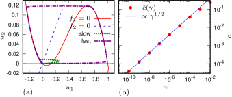
Figure 1: Propagating waves in the FHN model (19). (a) Phase plane of the point system with the null-clines and trajectories corresponding to the stable and unstable pulses, for ${\gamma}=10^{-3}$. (b) Speed of the critical (slow) pulse as function of ${\gamma}$, together with the theoretical asymptotic.

The scaling results of the previous section apply directly to this model, and thus serve as a method of verifying the numerical results under variations in the modal expansion length ${M}$, domain length ${L}$, and the application of projection boundary conditions, across several decades in ${\gamma}$. In particular, we find the expected asymptotic scaling of the wave components and pulse speed with ${\gamma}$ for ${L}\geq 50$ and ${M}\geq 32$, with exponentially small corrections to the leading eigenvalues for ${M}\geq 256$ when ${L}\geq 100$. For sufficiently small ${\gamma}$, the solution of the marginal eigenvalue ${\sigma_{2}}=0$ is eventually corrupted by the proximity of the essential spectrum of the wave to this eigenvalue, and the eigenfunctions ${\mathbf{v}_{2}}$ and ${\mathbf{w}_{2}}$ may not be computed using these methods; while ${M}$ and ${L}$ dependent, we have found this to occur for ${\gamma}<10^{-10}$, placing a limit on the reliability of the numerical approach taken in this work. Figure 1 demonstrates the correct scaling of the pulse speed ${\hat{{c}}}$ with ${\gamma}$, with good agreement with the ${\gamma}^{1/2}$ behavior for small ${\gamma}$.

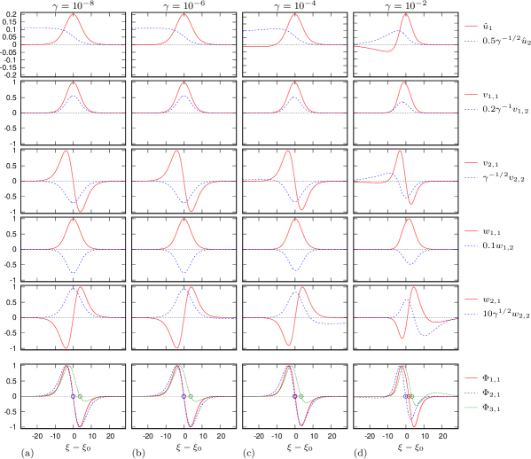
Figure 2: Scaled ingredients of the linearized theory for the FHN model (19) with varying ${\gamma}$ as specified above the columns. The coordinate ${\xi}={\xi_{0}}$ corresponds to the position of the maximum of ${\hat{u}_{1}}$. The open circles the panels in the bottom row indicate position of the zeros of the corresponding shift selectors.

Figure 2 summarizes the scaling of the components of the linear theory across six decades of ${\gamma}$, additionally showing the fast component of the constructed ${\mathbf{\Phi}_{{\ell}}}$. Note that since the perturbation is along the fast component, only the fast components of the shift selector, ${\Phi_{{\ell},1}}$, are relevant. Despite the correct observed scaling of the critical pulse ${\hat{{\mathbf{u}}}}$ and leading eigenfunctions ${\mathbf{v}_{1}}$, ${\mathbf{v}_{2}}$, ${\mathbf{w}_{1}}$, ${\mathbf{w}_{2}}$, the construction of ${\mathbf{\Phi}_{{\ell}}}$ indicates a subtlety in the selection of an optimal frame for the prediction of critical perturbations. While ${\mathbf{\Phi}_{1}}$ and ${\mathbf{\Phi}_{2}}$ converge to antisymmetric functions centered about the maximum of ${\hat{u}_{1}}$, ${\mathbf{\Phi}_{3}}$ instead converges to an asymmetric function whose central root remains offset from ${\xi}={\xi}_{0}$ in the limit ${\gamma}\to 0$. Considering the components of ${\mathbf{\Phi}_{3}}$ as defined in (LABEL:eq:Phil), we recognize that the contribution proportional to ${\mathbf{w}_{1}}$ does not monotonically vanish as ${\gamma}\to 0$, as originally expected in the formulation of the linear theory Bezekci-Biktashev-2017 which assumed identity of the ${\gamma}\to 0$ limit with the ${\gamma}=0$ “critical pulse” case.

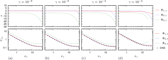
Figure 3: Shifts ${s}$ predicted by the three different shift selectors ${\mathbf{\Phi}_{{\ell}}}$ (upper row), and the corresponding predicted critical curves against the direct numerical simulations (lower row), for the FitzHugh-Nagumo model (19).

The deviation in the central root of ${\mathbf{\Phi}_{3}}$ has implications for the selection of optimal reference frames and the critical perturbation amplitudes associated with them. Figure 3 shows the critical strengths over three decades of the parameterized width ${{x}_{s}}$, both predicted using ${\mathbf{\Phi}_{{\ell}}}$ and computed using direct numerical simulation. The figure also shows the selection of the optimal frame shift ${s}$ for each of the predictions, in particular the systematic offset of ${s}_{3}$ as ${{x}_{s}}\to 0$, which coincides with the central root of ${\mathbf{\Phi}_{3}}$. This systematic offset in the selection of the optimal frame becomes more severe as ${\gamma}\to 0$, indicating that the prediction due to ${\mathbf{\Phi}_{3}}$ does not converge (this is not evident from the figure as presented but confirmed by careful observation of raw data). We conclude that as far as ${\mathbf{\Phi}_{3}}$ is concerned, the slow-fast system with ${\gamma}\to 0$ and the single-variable fast system dynamics of ${u_{1}}$ in isolation are qualitatively different, i.e., this is a singular limit. Further, it indicates that predictions made at large ${\gamma}$ are in fact more accurate than those made for smaller ${\gamma}$, which is reflected in the figure. Notably, for all observed values of ${\gamma}$, ${\mathbf{\Phi}_{3}}$ fails to recover the large (${{x}_{s}}\to\infty$) perturbation limit. A superficial interpretation of this small paradox is that in the ${\gamma}\to 0$ limit, all the events that decide the fate of a particular perturbation happen at the time scale $\mathcal{O}\!\left(1\right)$, so the slow variable remains almost at its resting value, whereas the heuristic behind ${\mathbf{\Phi}_{3}}$ is based on the matching of the initial condition against the critical pulse in full, i.e. taking into account both components. In the critical pulse, the slow variable is different from the resting value; although this difference is small, the sensitivity of the pulse position to the perturbation in the slow component, measured by ${w_{2,2}}$, is on the contrary large in this limit, hence the overall contribution of the slow component does not vanish in the limit ${\gamma}\to 0$.

A small, but nonetheless important note is that the predictive power of the linear theory is sensitive to the monotonicity and the root structure of ${\mathbf{\Phi}_{{\ell}}}$ for some perturbation widths, to the extent that the dependence of predicted ${s}$ and ${U_{s}}$ on ${{x}_{s}}$ is discontinuous. Such discontinuity occurs, for example, when a branch of ${\mu_{{\ell}}}({s})=0$, while continuing in ${{x}_{s}}$, terminates in a fold. In the vicinity of the fold value of ${{x}_{s}}$, the solution $({s},{U_{s}})$ on one side of the fold may differ significantly from the solution determined on the other side of the fold.

This appears in the linear theory prediction utilizing ${\mathbf{\Phi}_{3}}$, i.e. fig. 3, for ${\gamma}=10^{-2}$. For ${{x}_{s}}\gtrsim 25$ the linear theory makes no reasonable predictions for ${U_{s}}$, and for $5\lesssim{{x}_{s}}\lesssim 25$ the prediction for ${U_{s}}$ diverges from the asymptotic value correctly predicted by ${\mathbf{\Phi}_{1}}$ and ${\mathbf{\Phi}_{2}}$. The mechanical reason for this deviation is that the correlation integral defining ${\mu_{{\ell}}}$ corresponds to a box filter or smoothing operation, and for sufficiently large ${{x}_{s}}$ this smoothing is destructive. This smoothing destroys the delicate root structure seen in ${\mathbf{\Phi}_{3}}$ for ${\gamma}=10^{-2}$; so that while for ${{x}_{s}}\to 0$ the correlation integral forms a translation operation (preserving the number of roots), when the box filter width ${{x}_{s}}$ is comparable to the distance between successive roots of a function, the result of the correlation integral may have fewer roots, and specifically, it may only have roots which produce anomalously large predictions for ${U_{s}}$.

IV.2 Mitchell-Schaeffer

The Mitchell-Schaeffer Mitchell-Schaeffer-2003 model is a popular semi-conceptual model of cardiac cells, combining the simplicity of only two components with the relatively realistic description of action potential shape and restitution properties. Historically, it has been derived via an asymptotic reduction (adiabatic elimination of the fastest processes) of the more detailed Fenton-Karma model of atrial excitation, but still incorporates multiple decay timescales for the system. We re-write the kinetics of the model in the form

$${f_{1}} =(1-{u_{1}}){u_{1}}^{2}{u_{2}}-{u_{1}}{\tau_{i}}/{\tau_{u}},$$ (20)

$${f_{2}} =\left((1-{\theta}({u_{1}}))(1-{u_{2}})({\tau_{c}}/{\tau_{o}})-{\theta}({u_{1}}){u_{2}}\right),$$

where ${\theta}({u_{1}})=\mathrm{H}_{k}({u_{1}}-{u_{g}})=\left\{1+\tanh\left[{k}({u_{1}}-{u_{g}})\right]\right\}/2$ is a smoothed Heaviside distribution centered at ${u_{1}}={u_{g}}$ with width ${k}^{-1}$, and the timescales ratio in terms of the original parameters is ${\gamma}=({\tau_{i}}/{\tau_{c}})$ in this rescaling. The standard parameter values are ${\tau_{i}}=0.3\,\mathrm{ms}$, ${\tau_{o}}=120\,\mathrm{ms}$, ${\tau_{u}}=6\,\mathrm{ms}$, ${\tau_{c}}=150\,\mathrm{ms}$, ${u_{g}}=0.03$ and ${k}=100$. In the following examples, the parameter ratios ${\tau_{i}}/{\tau_{u}}=0.05$ and ${\tau_{c}}/{\tau_{o}}=1.25$ are kept at standard values, while ${\gamma}$ is treated as a free parameter. That is, for the purpose of the asymptotic theory, all of ${\tau_{i}}/{\tau_{u}}$, ${u_{g}}$ and ${k}^{-1}$ are treated as finite even though they are “small” in layman’s terms. The time ${t}$ is dimensionless as presented, likewise we absorb the original diffusion coefficient in the non-dimensional spatial scale, ${x}$.

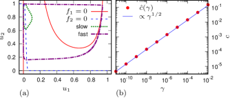
Figure 4: Propagating waves in the Mitchell-Schaeffer model (20). (a) Phase plane of the point system with the null-clines and trajectories corresponding to the stable and unstable pulses, for ${\gamma}=10^{-3}$. (b) Speed of the critical (slow) pulse as function of ${\gamma}$, together with the theoretical asymptotic.

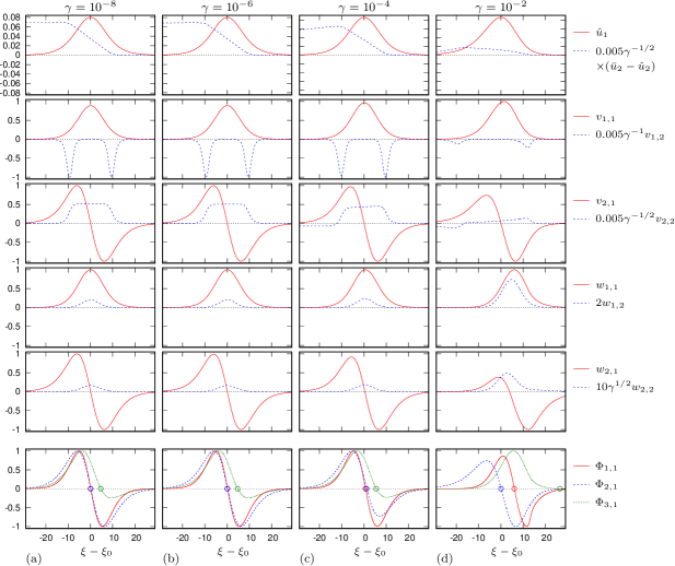
Figure 5: Scaled ingredients of the linearized theory for the Mitchell-Schaeffer model with varying ${\gamma}$ as specified above the columns. The coordinate ${\xi}={\xi_{0}}$ corresponds to the position of the maximum of ${\hat{u}_{1}}$. The thin vertical lines on the panels in the bottom row indicate position of the zeros of the corresponding shift selectors.

The scaling of the critical pulse and associated leading eigenfunctions in the Mitchell-Shaeffer model follow the expected scaling, see fig. 4 and fig. 5, similar to the FitzHugh-Nagumo model, while reproducing more realistic action potentials and gate switching dynamics. However, while the localization of the critical pulse in the fast variable (${u_{1}}$) is not dissimilar to the critical pulse in FitzHugh-Nagumo, the relative scale of the components of the leading eigenfunctions are reversed. Namely, we note that in relative terms, the second components of ${\mathbf{v}_{1}}$ and ${\mathbf{v}_{2}}$ are two orders of magnitude larger than would be expected based on their asymptotic order in ${\gamma}$ alone. This is related to the above mentioned non-asymptotic small parameters in the model, specifically, sharp switching of the ${f_{2}}$ across ${u_{1}}={u_{g}}$.

The shape of ${\mathbf{\Phi}_{1}}$ and ${\mathbf{\Phi}_{2}}$ are standard – both are approximately antisymmetric about the peak of the wave, see the bottom row in fig. 5. However, the contribution in the term proportional to ${\mathbf{w}_{1}}$ in ${\mathbf{\Phi}_{3}}$ is again significant, so we should expect a similar offset root and likewise inaccurate predictions for this shift selector.

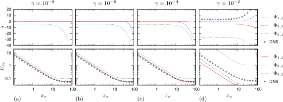
Figure 6: Shifts ${s}$ predicted by the three different shift selectors ${\mathbf{\Phi}_{{\ell}}}$ (upper row), and the corresponding predicted critical curves against the direct numerical simulations (lower row), Mitchell-Schaeffer.

The predicted critical excitation amplitudes ${U_{sc}}$ track the DNS results over three orders of magnitude for the extent of the perturbation, for the value computed using shift selectors ${\mathbf{\Phi}_{1}}$ and ${\mathbf{\Phi}_{2}}$. As expected, the predictions using the shifts determined by ${\mathbf{\Phi}_{3}}$ are much less accurate: they are systematically larger than the DNS results by nearly an order of magnitude. Note that this error in ${U_{sc}}$ is caused by a deviation of ${s}$ by only a fraction of the critical pulse width off the predictions of the other two shift selectors.

Comparison of the predicted results for large ${\gamma}$ indicates that it is the proximity of the central root of ${\mathbf{\Phi}_{{\ell}}}$ to the position of the peak of the unstable pulse which determines the effectiveness of the prediction, c.f., fig. 5. However, careful examination of fig. 6 indicates that between ${\gamma}=10^{-4}$ and ${\gamma}=10^{-2}$ the primacy of the different shift selectors changes; that is, at ${\gamma}=10^{-4}$, we see that ${\mathbf{\Phi}_{2}}$ is the most accurate shift selector, while at ${\gamma}=10^{-2}$ it is ${\mathbf{\Phi}_{1}}$ though no shift selector generates satisfactorily accurate predictions.

Taking note of fig. 6 for ${\gamma}=10^{-2}$, we observe that ${\mathbf{\Phi}_{3}}$ predicts critical excitation strengths which fail for ${{x}_{s}}>11$, i.e., for some sufficiently wide perturbations the branch of ${\mu_{3}}({s})=0$ ends in a fold, just as with the FHN model results. This mechanism thus appears to be a generic feature of qualitatively similar inputs to the infrastructure of the linear theory. It remains to determine the conditions under which ${\Phi_{3,1}}$ changes shape sufficiently that the convolution with the perturbation in the formation of ${\mu_{3}}$ destroys the optimal root. In principle, we may consider a toy model of the dependence ${\Phi_{3,1}}({s};{\gamma})$, in the form ${\varphi}({s};{a})={a}{w_{1,1}}({s})+\sqrt{1-{a}^{2}}{w_{2,1}}({s})$, whereby ${\varphi}({s};1)$ has no roots, while ${\varphi}({s};0)$ has a single root which persists under convolution with the perturbation ${\hat{\bar{\mathbf{X}}}}$ with a fixed, large, width ${{x}_{s}}$. At some intermediate value of ${a}={a}_{c}$, the number of roots in the convolution changes, which may be distinct from the value of ${a}={a}^{c}$ at which the number of roots within a central region of the domain of ${\varphi}(\,\cdot\,;{a})$ changes. The disparity between ${a}_{c}$ and ${a}^{c}$ suggests an analogous liminal region in which the time-scale separation ${\gamma}$ yields ${\Phi_{3,1}}$ with an appropriate root, but no corresponding root in ${\mu_{3}}$.

Indeed, fig. 6 suggests that for a given ${{x}_{s}}$, we may select a frame which precisely reflects the DNS results, that is, the actual position of the critical nucleus observed as a long transient when the perturbation magnitude is at its closest to the critical value. We say that this makes a postdictive optimal frame through the determination of ${s}{{}_{\mathrm{DNS}}}$, effectively. The relevant value of ${\gamma}=10^{-2}$ presents a situation in which all three predictive curves are distinct and each badly represents the DNS results. Iterating through perturbation extents we find that ${s}{{}_{\mathrm{DNS}}}>{s}_{2}>{s}_{1}>{s}_{3}$ over three decades of ${{x}_{s}}$. In the limit of ${{x}_{s}}\to 0$, $\lim{s}{{}_{\mathrm{DNS}}}\approx+3.47$, while $\lim{s}_{1}\approx-5.94$, $\lim{s}_{2}\approx 0.00$, and $\lim{s}_{3}\approx-26.4$. This exercise informs about the neighborhood of the predictive measures, however extending this observation to a general principle, i.e. generating a ${\mathbf{\Phi}}{{}_{\mathrm{DNS}}}$, is far from obvious.

IV.3 Modified “cubic recovery” FitzHugh-Nagumo

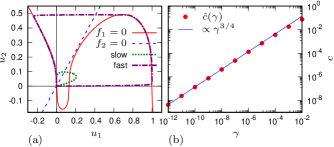
Figure 7: Propagating waves in the FHNCR model (21). (a) Phase plane of the point system with the null-clines and trajectories corresponding to the stable front and the unstable pulse, for ${\gamma}=10^{-3}$. (b) Speed of the critical (slow) pulse as function of ${\gamma}$, together with the theoretical asymptotic.

Here we consider a modification of the FitzHugh-Nagumo model (19) which is motivated by the nonlinear dependence of ${f_{1}}$ on ${u_{2}}$ in the Karma model considered in the next subsection. Our modified FHN model is

$${f_{1}} ={u_{1}}(1-{u_{1}})({u_{1}}-{\beta})-{u_{2}}^{q},$$ (21)

$${f_{2}} ={\alpha}{u_{1}}-{u_{2}}.$$

Obviously, (19) corresponds to the case ${q}=1$. In this subsection, we shall look at ${q}=3$ instead. We refer to this model as “FHN with cubic recovery” or FHNCR for short. We keep ${\beta}=0.131655$ as in (19), but take ${\alpha}=1.2$ in order to keep the kinetics excitable, i.e. have only one equilibrium, see fig. 7(a).

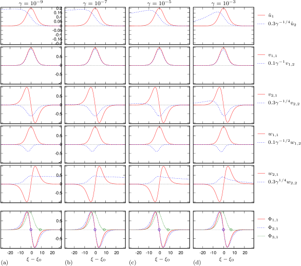
Figure 8: Scaled ingredients of the linearized theory for the FHNCR model (21) with varying ${\gamma}$ as specified above the columns. Notations are the same as in fig. 2.

Due to the degenerate dependence of ${f_{1}}$ on ${u_{2}}$, this model has different asymptotic properties, discussed in Subsection II.4. As expected from the results of that subsection, the pulse speed scales as ${\gamma}^{3/4}$, giving relatively fast convergence of the pulse to a static nucleus state, see fig. 7(b). Meanwhile, ${u_{2}}\sim{\gamma}^{1/4}$, see fig. 8 (top row) — a much slower convergence than standard FHN (${q}=1$). Recall the pulse solution ${\hat{{\mathbf{u}}}}$ asymptotically converges to the critical nucleus solution ${\mathbf{u}}=[{\phi},0]$ as ${\gamma}\to 0$. Similarly, slower convergence is observed for components ${v_{2,1}}$, ${w_{2,1}}$, and the component ${w_{1,1}}$ asymptotically vanishes unlike its counterpart in FHN model. This is all in agreement with the predictions from Subsection II.4. We are of course mostly interested in how this difference affects the accuracy of the lineary theory predictions for the critical curves.

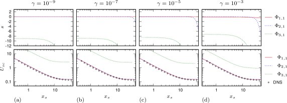
Figure 9: Shifts ${s}$ predicted by the three different shift selectors ${\mathbf{\Phi}_{{\ell}}}$ (upper row), and the corresponding predicted critical curves against the direct numerical simulations (lower row), for the FHNCR model (21).

The FHNCR model results should be read in dialogue with the FHN (${q}=1$) model results. As a point of concrete comparison, consider ${\gamma}=10^{-8}$ and ${{x}_{s}}\gg 10$ in the FHN model, fig. 3, where the frame selector ${\mathbf{\Phi}_{3}}$ predicts an amplitude which is approximately twice as large as the DNS result. Compare to the same configuration for the FHNCR model results for ${\gamma}=10^{-7}$ and ${\gamma}=10^{-9}$, fig. 9, which predicts a critical amplitude which is an order of magnitude larger than the DNS result, and five times larger than the linear model prediction. While the frame shifts selected by the ${\mathbf{\Phi}_{3}}$ condition prove significantly worse for FHNCR than for linear FHN, the frames selected by ${\mathbf{\Phi}_{1}}$ and ${\mathbf{\Phi}_{2}}$ are perfectly adequate predictors for the critical amplitude for both models. That is, the predictive power of the linear theory is not affected by the relative scaling of the components so long as a frame selecting heuristic is chosen carefully.

Further, numerical experiments with the FHNCR (not shown) suggest that, as ${q}$ increases further, we should expect the predictive power of ${\mathbf{\Phi}_{1}}$ and ${\mathbf{\Phi}_{2}}$ to outstrip that of ${\mathbf{\Phi}_{3}}$ more generally. Some slow-fast models of cardiac excitation, in particular, form a highly nonlinear (and indeed, parametric) dependence of ${f_{1}}$ on ${u_{2}}$. We consider one such model in the next subsection.

IV.4 Karma

The Karma-1994 Karma-1994 model is a qualitative model of cardiac excitation, designed to reproduce chosen restitution curves. The Karma model kinetics are given by the following functions,

$${f_{1}} =(({u^{*}}-{u_{2}}^{M})(1-\tanh({u_{1}}-{u_{d}})){u_{1}}^{2}/2-{u_{1}}),$$

$${f_{2}} ={\beta}\,\mathrm{H}_{k}({u_{1}}-{u_{a}})-{u_{2}},$$ (22)

where we will consider the parameter set ${u^{*}}=1.5415$, ${M}=4$, ${u_{d}}=3.0$, ${\beta}=1.389$, ${u_{a}}=0.5$, ${\tau_{1}}=2.5\,\mathrm{ms}$, ${\tau_{2}}=250\,\mathrm{ms}$, and in terms of the original notations of Karma-1994 we define ${\gamma}\equiv{\tau_{1}}/{\tau_{2}}$ as the ratio of timescales, so that ${t}$ is dimensionless. The original diffusion coefficient of the model is dimensional, we absorb this quantity in the non-dimensionalization of the spatial scale, ${x}$.

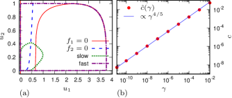
Figure 10: Propagating waves in the Karma model (IV.4). (a) Phase plane of the point system with the null-clines and trajectories corresponding to the stable and unstable pulses, for ${\gamma}=10^{-3}$. (b) Speed of the critical (slow) pulse as function of ${\gamma}$, together with the theoretical asymptotic.

Figure 10(a) sketches a phase portrait of the kinetics and fig. 10(b) shows the scaling of the speed of the unstable pulse solution for the Karma model. The pulse speed scales as ${\gamma}^{4/5}$, which matches the predictions of Subsection II.4; we of course have ${q}={M}$ here.

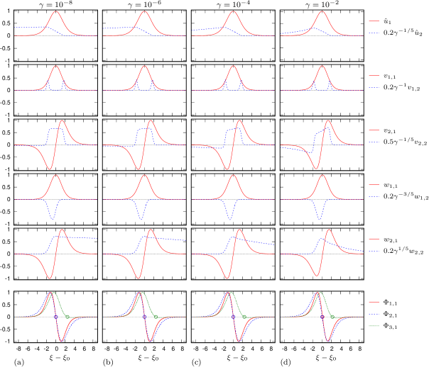
Figure 11: Scaled ingredients of the linearized theory for the Karma model with varying ${\gamma}$ as specified above the columns. The coordinate ${\xi}={\xi_{0}}$ corresponds to the position of the maximum of ${\hat{u}_{1}}$. The thin vertical lines on the panels in the bottom row indicate position of the zeros of the corresponding shift selectors.

Figure 11 summarizes the unstable pulse solution and leading eigenfunctions. As for the other models discussed above, the amplitude of ${u_{2}}$ decreases as ${\gamma}\to 0$; however, for Karma the convergence is significantly slower than the FHN or MS convergence rates. The convergence of the slow components of the leading left eigenfunctions is likewise complicated by the quartic dependence on ${u_{2}}$. In particular, the convergence rate for ${w_{1,2}}$ and for ${w_{2,2}}$ are markedly different, suggesting that for some intermediate value of ${\gamma}$ the dominant contribution to ${\Phi_{3,1}}$ switches from the term proportional to ${w_{2,1}}$ to the term proportional to ${w_{2,2}}$, and that predictions made on one side of the scale of ${\gamma}$ will contradict predictions made on the other, or asymptotically. A simple calculation suggests that this occurs for very large ${\gamma}$, when the asymptotic argument no longer holds.

While it is generically true that the structure of the leading eigenfunctions of the unstable pulse changes as ${\gamma}\to 0$, for the generic models considered previously the localization of the eigenfunction components are convergent for sufficiently small ${\gamma}$. For the FHNCR and Karma models, the leading right eigenfunctions (${\mathbf{v}_{1}}$, ${\mathbf{v}_{2}}$) and the leading left eigenfunction (${\mathbf{w}_{1}}$) are well-behaved in the limit of small ${\gamma}$. Both the leading right eigenfunctions (${\mathbf{v}_{1}}$, ${\mathbf{v}_{2}}$) are localized to the same region as the pulse, i.e., the leading right eigenfunctions inherit their localization from the nonlinear solution. Likewise, ${\mathbf{w}_{1}}$ is localized like ${\mathbf{v}_{1}}$ and the first components of these eigenfunctions coincide in the limit of small ${\gamma}$. However, as ${\gamma}\to 0$, the slow component of ${\mathbf{w}_{2}}$, ${w_{2,2}}$, behaves qualitatively differently. While for the generic models, ${w_{2,2}}$ converges to a localized function which decays quickly outside of the central region of the unstable pulse, for the degenerate models it does not. As ${\gamma}\to 0$, ${w_{2,2}}$ delocalizes asymmetrically, such that $\left\lvert{w_{2,2}}({\xi})\right\rvert>0$ ahead of the excited region of ${u_{1}}$, while $\left\lvert{w_{2,2}}({\xi})\right\rvert\to 0$ behind the peak.

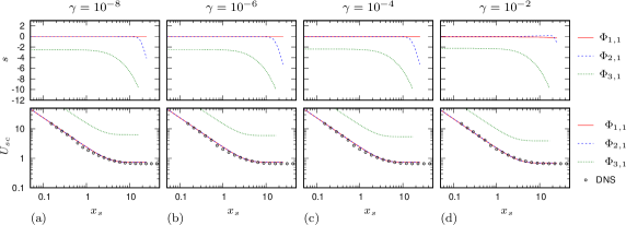
Figure 12: Shifts ${s}$ predicted by the three different shift selectors ${\mathbf{\Phi}_{{\ell}}}$ (upper row), and the corresponding predicted critical curves against the direct numerical simulations (lower row), Karma model.

The Karma model results represent a stress-test for the asymptotic scaling, both in terms of the stiffness of the kinetics and the parametric nonlinear dependence of ${f_{1}}$ on ${u_{2}}$. The former specifically marks the asymptotic structure of the pulse as an approximately piecewise linear curve, and the small-${\gamma}$ structure of the leading right eigenfunctions as wildly deviant from the other, smoother, models described in this work. The latter presents an opportunity to test the efficacy of the asymptotic analysis for severe nonlinearity.

In addition to the quartic nonlinearity (${M}=4$) results presented here, we also computed the asymptotic scaling of the linear theory ingredients for ${M}=2$, ${M}=8$, ${M}=16$, and ${M}=32$. In each instance of the parameterized model, the scaling of each component follows the predicted asymptotics described in Subsection II.4. As with the comparison of the cubic and linear FHN model critical curve predictions, as the nonlinearity ${M}$ increases, the less accurate ${\mathbf{\Phi}_{3}}$ becomes, while ${\mathbf{\Phi}_{1}}$ and ${\mathbf{\Phi}_{2}}$ maintain their predictive power across several decades of ${{x}_{s}}$ and ${\gamma}$.

V Discussion

The mathematical problem addressed here

is that of conditions required for initiation of a propagating excitation wave by an instant perturbation from the resting state by a stimulus of a certain spatial extent. The gist of our approach, previously exposed in Idris-Biktashev-2008 ; Biktashev-Idris-2008 ; Bezekci-etal-2015 ; Bezekci-2016 ; Bezekci-Biktashev-2017 ; Bezekci-Biktashev-2020 , is in linearization of the PDE system around a critical solution. A delicate issue is translational invariance of the problem which generates a one-parametric family of critical solutions, and poses a problem of identification of the member of that family that corresponds to a given initial perturbation. In the previous works, this issue was addressed by an heuristic suggesting that the initial condition of the linearized problem should not contain the shift mode. In this framework, the essential ingredients of the linearized theory, apart from the critical solution itself, are the right and left eigenfunctions of the linearization, corresponding to the first two eigenvalues, the first positive eigenvalue responsible for the instability of the critical solution, and the second being the zero eigenvalue corresponding to the translational symmetry. In particular, the left eigenfunction corresponding to the zero eigenvalue serves as the projector onto the shift mode.

In this paper, the focus is on four selected two-component systems with slow-fast time scale separation, like in FitzHugh-Nagumo model (FHN), including FHN model itself. In this class of models, the critical solution is a slow unstable propagating pulse. The results presented here were originally thought of as no more than further tests of applicability of the above mentioned approach in a particular class of models. This aim has been broadly achieved, however certain unexpected aspects have been revealed, which may serve as valuable lessons both for the specific problem but also at large for the theory of slow-fast systems.

The expectation

was to verify an asymptotic theory Bezekci-Biktashev-2017 based on the would-be obvious assumption that in the asymptotic limit, the events in the fast subsystem dominate, and therefore the predictions of the linearized theory should converge to those for the one-component system, in which the slow variable is frozen at the resting state value. Specifically, it was expected that the critical pulse solution converge to the stationary unstable non-uniform “critical nucleus” solution of the fast subsystem, and the eigenfunctions correspondingly converge to those of the critical nucleus as far as the fast components are concerned, and the slow components be negligible in the asymptotic limit.

Lesson one: this expectation has proved wrong.

Although the critical pulse solution does indeed converge as expected, and the fast components of the eigenfunctions indeed converge as expected, but the slow component paradoxically does not become negligible. Specifically, the slow component of the second left eigenfunctions, which is the projector to the translational mode and is therefore material for the heuristic used for critical pulse selection, grows large in the slow-fast asymptotic limit. This eigenfunction corresponds to sensitivity of the speed of the propagating pulse to perturbations of the slow component ahead of it, and increases and spreads out in sync with slow-down of that component. As a result, the overall contribution of the slow component in the overlap integral, coming from the left and right eigenfunction, does not vanish in the asymptotic limit, and although the predictions based on ignoring the slow components work reasonably well, as it appeared in the analysis done in Bezekci-Biktashev-2017 , the non-vanishing contribution from the slow component creates a systematic error in identifying the critical pulse, which considerably spoils prediction and in some cases renders the theory inappicable in principle.

Lesson two: there are other heuristics which do withstand the asymptotic limit.

Heuristics are required in our approach because of its leading idea to use linearization in the situation where the solution in question is in fact not small. The old heuristic, which has been in use since Biktashev-Idris-2008 , was to make the linearization “more applicable”, by making sure that its initial condition is “as small as possible” in the sense that in the critical situation, i.e. at the margin between successful and unsuccessful initiation, not only the first generalized Fourier component vanishes, which is a condition of criticality, but the second component vanishes, too, which is always achievable by an appropriate translation of the critial solution with respect to the initiation stimulus. There are of course may other senses in which the initial condition can be made “as small as possible”, offering alternative heuristics. In here we have explored two of them, one that minimizes the initial condition of the linearized problem in $L^{2}$ norm, and the other that minimizes the predicted threshold given by the criticality condition. Both new heuristics do not depend on the second left eigenfunction, and both have shown expectable convergence in the asymptotic limit, i.e. to the critical nucleus results, and good predictive ability, i.e. correspondence with the direct numerical simulations.

Lesson three: asymptotics may not give good predictions even when the asymptotic parameter, the ratio of time scales, is indeed very small.

This of course can happen if this is not the only small parameter in the problem, but there are others, such as other time scale ratios, or sharpness of transitions in the reaction kinetics, as we have seen in the examples of Mitchell-Schaeffer and Karma-1994 models. In such cases, the range of applicability of the asymptotics depends on those other parameters, and may be well away from realistic parameter ranges.

Lesson four: not all asymptotics are the same.

The natural genericity assumptions about the dependence of the kinetics terms on the dynamic variables may fail, leading to completely different asymptotics in the slow-fast limits. A priori this possibility might seem remote, but the fact that we have stumbled on such a failure “by accident” in a popular, even if simplified, cardiac excitation model Karma-1994 suggests that this possibility should be kept in mind. The slow rate of convergence in the fast/slow time scale separation parameter, particularly together with other small parameters present in the model, may render the fast/slow asymptotics irrelevant, in the sense that the behaviour of the solution at the original parameter value may be rather far from the asymptotic one, even though the original parameter value appear rather small.

Further directions.

Straightforward extension of this study would be to slow-fast systems with more than one fast and/or more than one slow component with similar, Tikhonov type occurrence of the small parameter. Note that even within this paradigm, there may be qualitatively different types of excitability Wieczorek-etal-2011 ; Hesse-etal-2017 . A still more intriguing possibility is about asymptotics in case of non-Tikhonov slow-fast models, of the kind discussed in Biktashev-Suckley-2004 ; Biktashev-etal-2008 ; Simitev-Biktashev-2011 . The known difference of systems with non-Tikhonov structure is that the asymptotic limit of the critical solution is not a stationary “nucleus”, but a moving front. Applicability of the linearized theory has been tested on a conceptual model of such critical front in Biktashev-Idris-2008 ; Bezekci-etal-2015 . However, convergence of the ingredients of the linearized theory and of corresponding predictions for the critical curves has not been explored so far to our knowledge. Given the lessons from the FitzHugh-Nagumo type systems discussed above, one should not take such convergence for granted. This direction is particularly important since non-Tikhonov asymptotics have been argued to better represent the properties of realistic ionic models of cardiac excitation, than FitzHugh-Nagumo type systems, particularly at the margins of propagation.

Implications of the observations presented here are also relevant for exotic solutions of one dimensional excitable models. We have noted that the convergence of the slow component of ${\mathbf{w}_{2}}$ is different for the generic and degenerate models, not only in the scaling of the solution near the asymptotic, but the asymptotic shape itself for small ${\gamma}$. To reiterate, ${w_{2,2}}$ is asymmetrically extended for $x$ ahead of the pulse peak, while decays to zero quickly behind the pulse peak. This feature of ${\mathbf{w}_{2}}$ in conjunction with the localization of ${\mathbf{w}_{1}}$ suggests that the slow dynamics (the physically relevant dynamics) of the unstable pulse are nearly insensitive to perturbations positioned post-peak, but very sensitive to being slowed by perturbations almost arbitrarily ahead of the pulse peak. This may play an important role in the development of “back-initiation”, or the observability of a “one-dimensional spiral” solution generally Cytrynbaum-Lewis-2008 . The extension of ${w_{2,2}}$ should lead to acceleration of newly created pulse formations ignited by back-initation and increase the potential for local collapse to the resting state. As we know such an unstable solution exists in FHN-type models, one would expect that the increased sensitivity of an extended ${w_{2,2}}$ may suppress the formation of these dynamics, suggesting that degenerate models may have more complex saddle structures.

One natural extension of the existing program is to the “critical quenching problem”, that is, of cessation of stable wave propagation in an excitable medium by addition of minimally invasive perturbations. The application to quenching is an inversion of the application to ignition, though the central ingredients can be the same and rely on the same linearization about the unstable pulse state. Crucially, as quenching considers an equivariant state in the form of the stable wave, as compared to the invariant quiescent state, the problem involves the consideration of an additional parameter which fixes the additional translational symmetry. This problem will be addressed in a forthcoming paper.

- [1] B. Bezekci, I. Idris, R. D. Simitev, and V. N. Biktashev. Semi-analytical approach to criteria for ignition of excitation waves. Phys. Rev. E, 92(4):042917, 2015.
- [2] R. FitzHugh. Impulses and physiological states in theoretical models of nerve membrane. Biophysical Journal, 1(6):445–466, 1961.
- [3] A. Karma. Electrical alternans and spiral wave breakup in cardiac tissue. Chaos, 4(3):461–472, 1994.
- [4] C. C. Mitchell and D. G. Schaeffer. A two-current model for the dynamics of cardiac membrane. Bull. Math. Biol., 65(5):767–793, 2003.
- [5] W.-J. Beyn. The numerical computation of connecting orbits in dynamical systems. IMA J. Num. Anal., 10(3):379–405, 1990.
- [6] E. Doedel and J. P. Kernevez. AUTO, software for continuation and bifurcation problems in ordinary differential equations, 1986.
- [7] K. J. Burns, G. M. Vasil, J. S. Oishi, D. Lecoanet, and B. P. Brown. Dedalus: A flexible framework for numerical simulations with spectral methods. http://arxiv.org/abs/1905.10388, 2019.
- [8] U. M. Ascher, S. J. Ruuth, and R. J. Spiteri. Implicit-explicit Runge-Kutta methods for time-dependent partial differential equations. Applied Numerical Mathematics, 25(2–3):151–167, 1997.
- [9] E. L. Ortiz. The tau method. SIAM Journal on Numerical Analysis, 6(3):480–492, 1969.
- [10] J. Guckenheimer and C. Kuehn. Homoclinic orbits of the FitzHugh-Nagumo equation: The singular limit. Discrete and Continuous Dynamical Systems - Series S, 2(4):851–872, 2009.
- [11] G. Flores. Stability analysis for the slow travelling pulse of the FitzHugh–Nagumo system. SIAM Journal on Mathematical Analysis, 22(2):392–399, 1991.
- [12] J. J. Tyson and J. P. Keener. Singular perturbation theory of traveling waves in excitable media (a review). Physica D, 32(3):327–361, 1988.
- [13] R. G. Casten, H. Cohen, and P. A. Lagerstrom. Perturbation analysis of an approximation to the Hodgkin-Huxley theory. Quarterly of Applied Mathematics, 32(4):365–402, 1975.
- [14] B. Bezekci and V. N. Biktashev. Fast-slow asymptotic for semi-analytical ignition criteria in FitzHugh-Nagumo system. Chaos, 27:093916, 2017.
- [15] I. Idris and V. N. Biktashev. Analytical approach to initiation of propagating fronts. Phys. Rev. Lett., 101:244101, 2008.
- [16] V. N. Biktashev and I. Idris. Initiation of excitation waves: An analytical approach. Computers in Cardiology, 35:311–314, 2008.
- [17] B. Bezekci. Analytical and Numerical Approaches to Initiation of Excitation Waves. PhD thesis, Exeter University, 2016.
- [18] B. Bezekci and V. N. Biktashev. Strength-duration relationship in an excitable medium. Communications in Nonlinear Science and Numerical Simulation, 80:104954, 2020.
- [19] S. Wieczorek, P. Ashwin, C. M. Luke, and P. M. Cox. Excitability in ramped systems: the compost-bomb instability. Proc. R. Soc. A, 467:1243–1269, 2011.
- [20] J. Hesse and J. Schleimer S. Schreiber. Qualitative changes in phase-response curve and synchronization at the saddle-node-loop bifurcation. Phys. Rev. E, 95:052203, 2017.
- [21] V. N. Biktashev and R. Suckley. Non-Tikhonov asymptotic properties of cardiac excitability. Phys. Rev. Lett., 93(16):168103, 2004.
- [22] V. N. Biktashev, R. Suckley, Y. E. Elkin, and R. D. Simitev. Asymptotic analysis and analytical solutions of a model of cardiac excitation. Bull. Math. Biol., 70(2):517–554, 2008.
- [23] R. D. Simitev and V. N. Biktashev. Asymptotics of conduction velocity restitution in models of electrical excitation in the heart. Bull. Math. Biol., 73(1):72–115, 2011.
- [24] E. N. Cytrynbaum and T. J. Lewis. A global bifurcation and the appearance of a one-dimensional spiral wave in excitable media. SIAM Journal on Applied Dynamical Systems, 8(1):348–370, 2009.