Basic Principles of Clustering Methods

Abstract

Clustering methods group a set of data points into a few coherent groups or clusters of similar data points. As an example, consider clustering pixels in an image (or video) if they belong to the same object. Different clustering methods are obtained by using different notions of similarity and different representations of data points.

I Introduction

We consider data points which can be represented by Euclidean vectors ${\bf x}=\big{(}x_{1},\dots,x_{n}\big{)}^{T}\in\mathbb{R}^{n}$. For digital images and videos such a representation can be obtained by stacking the red, green and blue intensities of pixels into a vector [1]. Data points obtained from sound signals can be transformed into vectors by sampling the signal with a certain sampling frequency. Music recordings are typically sampled at a rate of $44\cdot 10^{3}{\rm Hz}$ [2]. Wireless communication systems face data points in the form of time signals that represent individual transmit symbols. These time signals have to sampled at rates proportional to the radio bandwidth used in the wireless communication system [3]. Natural language processing deals with data points representing text documents, ranging from short text messages to entire document collection [4, 5].

In what follows, we assume that data points are given (represented) in the form of feature vectors ${\bf x}\in\mathbb{R}^{n}$. To have a concrete example in mind, we consider data points representing patches (rectangular regions) of the snapshot depicted in Figure 1. Each patch is characterized by the feature vector ${\bf x}=(x_{\rm red},x_{\rm green},x_{\rm blue})$ whose entries are the average redness $x_{\rm red}$, greenness $x_{\rm blue}$ and greenness $x_{\rm green}$ of all the pixels belonging to this patch. The entire dataset $\mathbb{X}=\{\mathbf{x}^{(i)}\}_{i=1}^{m}$ is given by all the feature vectors for the patches.

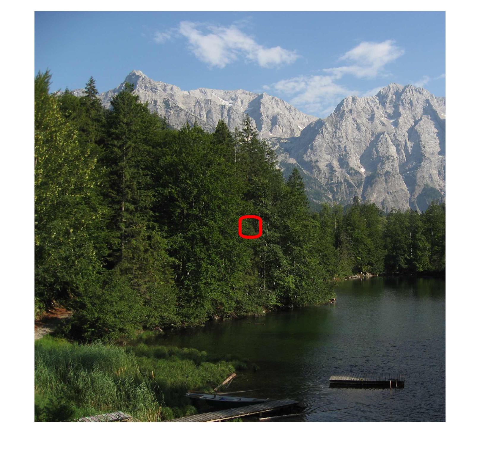
Figure 1: We consider data points obtained from small rectangular regions (“patches”) of a snapshot. One such patch is indicated by a red box.

Figure 2: Data points representing patches of the image in Figure 1. Each data point is depicted as a circle whose location is given by the average redness and blueness of the pixels in the corresponding image patch.

Clustering methods partition a dataset $\mathbb{X}=\{\mathbf{x}^{(i)}\}_{i=1}^{m}$, consisting of $m$ data points represented by the (feature) vectors $\mathbf{x}^{(i)}\in\mathbb{R}^{n}$, into a small number of groups or "clusters" $\mathcal{C}^{(1)},\ldots,\mathcal{C}^{(k)}$. Each cluster $\mathcal{C}^{(c)}$ represents a subset of data points which are more similar to each other than to data points in another cluster. The precise meaning of calling two data points "similar" depends on the application at hand. There are different notions of similarity that lead to different clustering methods.

Clustering methods do not require labeled data and can be applied to data points which are characterized solely by features $\mathbf{x}^{(i)}$. Therefore, clustering methods are referred to as unsupervised machine learning methods. However, clustering methods are often used in combination with (as a preprocessing step for) supervised learning methods such as regression or classification.

There are two main flavours of clustering methods:

• hard clustering methods assign each data point to exactly one cluster.

• soft clustering methods assign each data point to several different clusters but with varying degrees of belonging.

Hard clustering can be interpreted as a special case of soft clustering with the degrees of belonging enforced to be either zero (“no belonging”) or one (“full belonging”).

In Section II we discuss one popular method for hard clustering, the k-means algorithm. In Section III, we discuss one popular method for soft clustering, which is based on a probabilistic Gaussian mixture model (GMM). The clustering methods in Section II and Section III use a notion of similarity that is tied to the Euclidean geometry of $\mathbb{R}^{n}$. In some applications, it is more useful to use a different notion of similarity. Section IV discusses one example of a clustering method which uses a non-Euclidean notion of similarity.

II Hard Clustering

Hard clustering methods partition a dataset $\mathbb{X}=\{\mathbf{x}^{(1}),\ldots,\mathbf{x}^{(m)}\}$ into $k$ non-overlapping clusters $\mathcal{C}^{(1)},\ldots,\mathcal{C}^{(k)}$. Each data point $\mathbf{x}^{(i)}$ is assigned to precisely one cluster whose index we denote by $y^{(i)}\in\{1,\ldots,k\}$.

The formal setup of hard clustering is somewhat similar to that of classification methods. Indeed, we can interpret the cluster index $y^{(i)}$ as the label (quantity of interest) associated with the $i$ th data point. However, in contrast to classification problems, clustering does not require any labeled data points.

Clustering methods do not require knowledge of the cluster assignment for any data point. Instead, clustering methods learn a reasonable cluster assignment for a data point based on the intrinsic geometry of the entire dataset $\mathbb{X}$.

II-A $k$-means

Maybe the most basic (and popular) method for hard clustering is the $k$-means algorithm. This algorithm represents each (non-empty) cluster $\mathcal{C}^{(c)}\subseteq\mathbb{X}$ by the cluster mean

$$\mathbf{m}^{(c)}=(1/|\mathcal{C}^{(c)}|)\sum_{\mathbf{x}^{(i)}\in\mathcal{C}^{(c)}}\mathbf{x}^{(i)}.$$

If we would know the cluster means $\mathbf{m}^{(c)}$ for each cluster, we could assign each data point $\mathbf{x}^{(i)}$ to the cluster with index $y^{(i)}$ whose mean $\mathbf{m}^{(y^{(i)})}$ is closest in Euclidean norm,

$$\|\mathbf{x}^{(i)}-\mathbf{m}^{(y^{(i)})}\|=\min\limits_{c\in\{1,\ldots,k\}}\|\mathbf{x}^{(i)}-\mathbf{m}^{(c)}\|.$$

However, in order to determine the cluster means $\mathbf{m}^{(c)}$, we would have needed the cluster assignments $y^{(i)}$ already in the first place. This instance of an “egg-chicken dilemma” (see https://en.wikipedia.org/wiki/Chicken_or_the_egg) is resolved within the $k$-means algorithm by iterating the cluster means and cluster assignment update. We have summarized the $k$-means algorithm in Algorithm 1.

Algorithm 1 $k$-Means Clustering

1:data points $\mathbf{x}^{(1)},\ldots,\mathbf{x}^{(m)}$, number $k$ of clusters, initial cluster means $\mathbf{m}^{(c)}$ for $c=1,\ldots,k$.

2:Iterate

3:repeat

4:     update cluster assignments

$$y^{(i)}:=\operatorname*{argmin}\limits_{c\in\{1,\ldots,k\}}\|\mathbf{x}^{(i)}-\mathbf{m}^{(c)}\|\mbox{ for all }i=1,\ldots,m$$ (1)

5:     update cluster means

$$\mathbf{m}^{(c)}\!:=\!\frac{1}{\mid\{i:\!y^{(i)}\!=\!c\}\mid}\sum_{i:y^{(i)}\!=\!c}\mathbf{x}^{(i)}\mbox{ for all }c=1,\ldots,k$$ (2)

6:until stopping criterion is satisfied

7:cluster assignments $y^{(i)}$ for all $i=1,\ldots,m$

In order to implement Algorithm 1, we need to fix three issues that are somewhat hidden in its formulation. First, we need to specify how to break ties in the case when, for a particular data point ${\bf x}^{(i)}$, there are several cluster indices $c\!\in\!\{1,\ldots,k\}$ achieving the minimum in (1).

Second, we need to take care of a situation when after a cluster assignment update (1), some cluster $\mathcal{C}^{(c^{\prime})}$ has no data points associated with it,

$$|\{i:y^{(i)}=c^{\prime}\}|=0.$$ (3)

In this case, the cluster means update (2) would not be well defined for the cluster $\mathcal{C}^{(c^{\prime})}$. Finally, we need to specify a stopping criterion (“checking convergence”).

Algorithm 2 is obtained from Algorithm 1 by fixing those three issues in a particular way [6]. To this end, it maintains the cluster activity indicators $b^{(c)}\in\{0,1\}$, for $c=1,\ldots,k$. Whenever the assignment update (4) results in a cluster $\mathcal{C}^{(c)}$ with no data points assigned to it, the corresponding indicator is set to zero, $b^{(c)}=0$. On the other hand, if at least one data point is assigned to cluster $\mathcal{C}^{(c)}$, we set $b^{(c)}=1$. Using these additional variables allows to execute the cluster mean update step (5) only for clusters with at least one data point ${\bf x}^{(i)}$ assigned to it. The cluster assignment update step (4) breaks ties in (1) by preferring (other things being equal) lower cluster indices.

Algorithm 2 $k$-Means “Fixed Point Algorithm” in [6]

1:data points $\mathbf{x}^{(1)},\ldots,\mathbf{x}^{(m)}$, number $k$ of clusters, initial cluster means $\mathbf{m}^{(c)}$ for $c=1,\ldots,k$.

2:repeat

3:     update cluster assignments

$$y^{(i)}\!:=\!\min\{\operatorname*{argmin}\limits_{c^{\prime}\in\{1,\ldots,k\}}\|{\bf x}^{(i)}-{\bf m}^{(c^{\prime})}\|\}\mbox{ for all }i\!=\!1,\ldots,m$$ (4)

4:     update activity indicators

$$b^{(c)}:=\begin{cases}1&\mbox{ if }|\{i:y^{(i)}=c\}|>0\\ 0&\mbox{ else.}\end{cases}\mbox{ for all }c\!=\!1,\ldots,k,$$ (5)

5:     update cluster means

$${\bf m}^{(c)} :=\frac{1}{|\{i:y^{(i)}=c\}|}\sum_{i:y^{(i)}=c}{\bf x}^{(i)}$$

$$\mbox{ for all }c\!=\!1,\ldots,k\mbox{ with }b^{(c)}=1$$ (6)

6:until cluster assignments $y^{(i)}$ do not change

7:cluster assignments $y^{(i)}$

As verified in [6, Appendix C], Algorithm 2 is guaranteed to terminate within a finite number of iterations. In other words, after a finite number of cluster mean and assignment updates, Algorithm 2 finds a cluster assignments $\{y^{(i)}\}_{i=1}^{m}$ which is unaltered by any additional iteration of cluster mean and assignment update.

II-B Initialization

Figure 3: A dataset along with the subspace spanned by the principal direction. Data points are depicted by circles and the corresponding principal components by crosses.

Algorithm 1 requires as input some initial choices for the cluster means ${\bf m}^{(c)}$, for $c=1,\ldots,k$. Different strategies are used for choosing the initial cluster means. We can initialize the cluster means ${\bf m}^{(c)}$ by randomly selecting $k$ different data points ${\bf x}^{(i)}$ out of $\mathbb{X}$. Another option for initializing the cluster means is based on the principal components of the data points in $\mathbb{X}$. This principal component is found by projecting onto the principal direction

$$\mathbf{v}=\operatorname*{argmax}_{{\bf w}\in\mathbb{R}^{n}}(1/m)\sum_{i=1}^{m}\big{(}{\bf w}^{T}\mathbf{x}^{(i)}\big{)}^{2}.$$ (7)

The principal direction $\mathbf{v}$ spans the one-dimensional subspace $\{t\mathbf{v}:t\in\mathbb{R}\}$ which is the best approximation of $\mathbb{X}$ among all one-dimensional subspaces. The cluster means might then be chosen by evenly partitioning the value range of the principal components ${\bf v}^{T}{\bf x}^{(i)}$ for $i=1,\ldots,m$. Figure 3 depicts a dataset whose data points are indicated by circles and the subspace spanned by the principal direction as a line.

II-C Minimizing Clustering Error

Algorithm 1 can be interpreted as a method for minimizing the clustering error

$$\mathcal{E}(\{\mathbf{m}^{(c)}\}_{c=1}^{k},\{y^{(i)}\}_{i=1}^{m}\mid\{\mathbf{x}^{(i)}\}_{i=1}^{m})$$

$$=(1/m)\sum_{m=1}^{m}{\left\|\mathbf{x}^{(i)}-\mathbf{m}^{(y^{(i)})}\right\|^{2}}.$$ (8)

For convenience we will drop the explicit dependence of the clustering error (II-C) on the cluster means $\{\mathbf{m}^{(c)}\}_{c=1}^{k}$ and assignments $\{y^{(i)}\}_{i=1}^{m}$.

The means update (2) within Algorithm 1 amounts to minimizing $\mathcal{E}$ by varying the cluster means $\mathbf{m}^{(c)}$ for fixed assignments $y^{(i)}$. The assignment update (1) within Algorithm 1 amounts to minimizing $\mathcal{E}$ by varying the assignments $y^{(i)}$ with the cluster means $\mathbf{m}^{(c)}$ held fixed. Thus, the sequence of cluster means and assignments generated by Algorithm 1 decreases the clustering error (II-C).

Interpreting Algorithm 1 as an iterative method for minimizing (II-C) provides a natural choice for the stopping criterion in Algorithm 1. We could specify a threshold for the required (relative) decrease of the clustering error (II-C) achieved by one additional iteration of Algorithm 1. If the decrease of the clustering error (II-C) is smaller than this threshold, the iterations in Algorithm 1 are stopped.

Since the clustering error (II-C) is a non-convex function of the cluster means and assignments, Algorithm 1 might get trapped in a local minimum. It is therefore useful to repeat Algorithm 1 several times with different initializations for the cluster means and then choose the cluster assignment resulting in the smallest empirical risk among all repetitions.

III Soft Clustering

The cluster assignments obtained from hard clustering, such as Algorithm 2, provide rather coarse-grained information. Even if two data points ${\bf x}^{(i)},{\bf x}^{(j)}$ are assigned to the same cluster $c$, their distances to the cluster mean ${\bf m}^{(c)}$ might be very different (see Figure 4). For some applications, we would like to have a more fine-grained information about the cluster assignments.

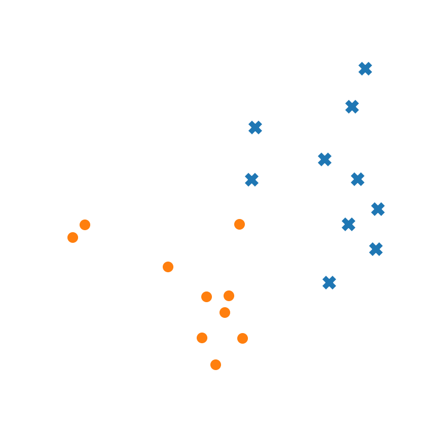
Figure 4: Hard clustering of data points. Some data points are closer to the boundary between clusters than others.

Soft-clustering methods provide such fine-grained information by explicitly modelling the degree (or confidence) by which a particular data point belongs to a particular cluster. More precisely, soft-clustering methods track for each data point ${\bf x}^{(i)}$ the degree of belonging to each of the clusters $c\in\{1,\ldots,k\}$.

III-A Gaussian Mixture Models

A principled approach to defining a degree of belonging to different clusters is to interpret each data point ${\bf x}^{(i)}$, for $i=1,\ldots,m$, as the realization of a random vector. The probability distribution the (random) data point ${\bf x}^{(i)}$ depends on the cluster to which this data point belongs. Formally, we represent each cluster $\mathcal{C}^{(c)}$ with a multivariate normal distribution [7]

$$\mathcal{N}({\bf x};{\bm{\mu}}^{(c)},{\bm{\Sigma}}^{(c)}) =$$

$$\frac{1}{\sqrt{{\rm det}\{2\pi{\bm{\Sigma}}\}}}\exp\big{(}-(1/2)({\bf x}\!-\!{\bm{\mu}})^{T}{\bm{\Sigma}}^{-1}({\bf x}\!-\!{\bm{\mu}})\big{)}$$ (9)

of a Gaussian random vector with mean ${\bm{\mu}}^{(c)}$ and (invertible) covariance matrix ${\bf\Sigma}^{(c)}$.

While $k$-means represents each cluster $\mathcal{C}^{(c)}$ by the cluster mean ${\bf m}^{(c)}$, here we represent each cluster by a probability distribution (III-A). However, since we restrict ourselves to multivariate normal (or Gaussian) distributions, we can parametrize the cluster-specific distributions (III-A) using a mean vector and a covariance matrix. In other words we only need to store a vector and a matrix to represent the entire probability distribution (III-A).

The index $c^{(i)}$ of the cluster from which data point ${\bf x}^{(i)}$ is generated is unknown. Therefore, we model the cluster index $c^{(i)}$ as a random variable with the probability distribution

$$p_{c}:={\rm P}({c^{(i)}=c})\mbox{ for }c=1,\ldots,k.$$ (10)

The (prior) probabilities $p_{c}$ are unknown and have to be estimated from observing the data points ${\bf x}^{(i)}$. If we knew the cluster index $c^{(i)}=c$ of the $i$th data point, the distribution of the vector ${\bf x}^{(i)}$ would be

$${\rm P}({{\bf x}^{(i)}|c^{(i)}=c})=\mathcal{N}\big{(}{\bf x};{\bm{\mu}}^{(c)},{\bm{\Sigma}}^{(c)}\big{)}$$ (11)

with mean vector ${\bm{\mu}}^{(c)}$ and covariance matrix ${\bm{\Sigma}}^{(c)}$.

The overall probabilistic model (11), (10) amounts to a Gaussian mixture model (GMM). Indeed, using the law of total probability, the marginal distribution ${\rm P}({{\bf x}^{(i)}})$ (which is the same for all data points ${\bf x}^{(i)}$) is a mixture of Gaussians,

$${\rm P}({{\bf x}^{(i)}})=\sum_{c=1}^{k}\underbrace{{\rm P}({y^{(i)}=c})}_{p_{c}}\underbrace{{\rm P}({{\bf x}^{(i)}|y^{(i)}=c})}_{\mathcal{N}({\bf x}^{(i)};{\bm{\mu}}^{(c)},{\bm{\Sigma}}^{(c)})}.$$ (12)

Figure 5 depicts a GMM using $k=3$ clusters.

It is important to note that the cluster assignments $y^{(i)}$ are hidden (unobserved) random variables. We thus have to infer or estimate these variables from the observed data points $\mathbf{x}^{(i)}$ which are i.i.d. realizations of the GMM (12).

Modelling the cluster assignments $c^{(i)}$ as (realizations of) random variables lends naturally to a precise definition for the degree of belonging to a particular cluster. In particular, we define the degree $y^{(i)}_{c}$ of data point ${\bf x}^{(i)}$ belonging to the cluster $\mathcal{C}^{(c)}$ as the “a-posteriori” probability of the assignment variable $c^{(i)}$ being equal to $c\in\{1,\ldots,k\}$,

$$y^{(i)}_{c}:={\rm P}({c^{(i)}=c|\mathbb{X}}).$$ (13)

For each data point ${\bf x}^{(i)}$, the degree of belonging (13) involves a conditioning on the entire dataset $\mathbb{X}$. This is reasonable since the degree of belonging for each data point typically depends on the overall (cluster) geometry of the entire dataset $\mathbb{X}$.

The degrees of belonging $y^{(i)}_{c}$ sum to one,

$$\sum_{c=1}^{k}y^{(i)}_{c}=1\mbox{ for each }i=1,\ldots,m.$$ (14)

Figure 5: The GMM (12) yields a probability density function which is a weighted sum of multivariate normal distributions $\mathcal{N}({\bm{\mu}}^{(c)},{\bm{\Sigma}}^{(c)})$. The weight of the $c$-th component is the cluster probability ${\rm P}({c^{(i)}=c})$.

III-B Expectation Maximization

Using the GMM (12) for explaining the observed data points ${\bf x}^{(i)}$ turns the clustering problem into a statistical inference or parameter estimation problem [8, 9]. We have to estimate (approximate) the true underlying cluster probabilities $p_{c}$ (see (10)), cluster means ${\bm{\mu}}^{(c)}$ and cluster covariance matrices ${\bm{\Sigma}}^{(c)}$ (see (11)) from the observed data points $\mathbb{X}=\{{\bf x}^{(i)}\}_{i=1}^{m}$, which are drawn from the probability distribution (12).

We denote the estimates for the GMM parameters by $\hat{p}_{c}(\approx p_{c})$, ${\bf m}^{(c)}(\approx{\bm{\mu}}^{(c)})$ and $\mathbf{C}^{(c)}(\approx{\bm{\Sigma}}^{(c)})$, respectively. Based on these estimates, we can then compute an estimate $\hat{y}_{c}^{(i)}$ of the (a-posterior) probability

$$y_{c}^{(i)}={\rm P}({c^{(i)}=c\mid\mathbb{X}})$$ (15)

of the $i$-th data point ${\bf x}^{(i)}$ belonging to cluster $c$, given the observed dataset $\mathbb{X}$.

It turns out that this estimation problem becomes significantly easier by operating in an alternating fashion: In each iteration, we first compute a new estimate $\hat{p}_{c}$ of the cluster probabilities $p_{c}$, given the current estimate ${\bf m}^{(c)},\mathbf{C}^{(c)}$ for the cluster means and covariance matrices. Then, using this new estimate $\hat{p}_{c}$ for the cluster probabilities, we update the estimates ${\bf m}^{(c)},\mathbf{C}^{(c)}$ of the cluster means and covariance matrices. Then, using the new estimates ${\bf m}^{(c)},\mathbf{C}^{(c)}$, we compute a new estimate $\hat{p}_{c}$ and so on. By repeating these two update steps, we obtain an iterative soft-clustering method which is summarized in Algorithm 3.

Algorithm 3 “A Soft-Clustering Algorithm” [10]

1:dataset $\mathbb{X}=\{{\bf x}^{(i)}\}_{i=1}^{m}$; number $k$ of clusters.

2:Initialize: use initial guess for GMM parameters $\{\mathbf{m}^{(c)},\mathbf{C}^{(c)},\hat{p}_{c}\}_{c=1}^{k}$

3:repeat

4:     for each data point ${\bf x}^{(i)}$ and cluster $c\in\{1,\ldots,k\}$, update degrees of belonging

$$y_{c}^{(i)} =\frac{\hat{p}_{c}\mathcal{N}({\bf x}^{(i)};\mathbf{m}^{(c)},\mathbf{C}^{(c)})}{\sum_{c^{\prime}=1}^{k}\hat{p}_{c^{\prime}}\mathcal{N}({\bf x}^{(i)};\mathbf{m}^{(c^{\prime})},\mathbf{C}^{(c^{\prime})})}$$ (16)

5:     for each cluster $c\in\{1,\ldots,k\}$, update estimates of

• cluster probability $\hat{p}_{c}\!=\!m_{c}/m$, with effective cluster size $m_{c}\!=\!\sum\limits_{i=1}^{m}y_{c}^{(i)}$

• compute cluster mean (estimate)

  $$\mathbf{m}^{(c)}=(1/m_{c})\sum\limits_{i=1}^{m}y_{c}^{(i)}{\bf x}^{(i)}$$

• compute cluster covariance matrix (estimate)

  $$\mathbf{C}^{(c)}=(1/m_{c}){\sum\limits_{i=1}^{m}y_{c}^{(i)}\big{(}{\bf x}^{(i)}\!-\!\mathbf{m}^{(c)}\big{)}\big{(}{\bf x}^{(i)}\!-\!\mathbf{m}^{(c)}\big{)}^{T}}$$

6:until convergence

7:soft cluster assignments ${\bf y}^{(i)}=(y_{1}^{(i)},\ldots,y_{k}^{(i)})^{T}$ for each data point ${\bf x}^{(i)}$

As with hard clustering (see Section II-C), we can also interpret soft clustering as an optimization problem. In particular, Algorithm 3 aims at choosing GMM parameter estimates $\{{\bf m}^{(c)},\mathbf{C}^{(c)},\hat{p}_{c}\}_{c=1}^{k}$ that minimize the soft clustering error

$$\mathcal{E}^{(\rm SC)}:=-\log{\rm P}({\mathbb{X};\{{\bf m}^{(c)},\mathbf{C}^{(c)},\hat{p}_{c}\}_{c=1}^{k}}).$$ (17)

The interpretation of Algorithm 3 as a method for minimizing the empirical risk (17) suggests to monitor the decrease of the empirical risk $\mathcal{E}^{(\rm SC)}$ to decide when to stop iterating (“convergence test”).

Similar to $k$-means Algorithm 1, also the soft clustering Algorithm 3 suffers from the problem of getting stuck in local minima of the empirical risk (17). Therefore, as for $k$-means Algorithm 1 (see Section II), one typically runs Algorithm 3 several times. Each run uses a different choice for the initial GMM parameters in Algorithm 3 and results in different estimates $\{{\bf m}^{(c)},\mathbf{C}^{(c)},\hat{p}_{c}\}_{c=1}^{k}$ for the GMM parameters. We then pick the GMM parameters obtained in the run achieving the smallest empirical risk (17).

We note that the empirical risk (17) underlying the soft-clustering Algorithm 3 is essentially a log-likelihood function. Thus, Algorithm 3 can be interpreted as an approximate maximum likelihood estimator for the true underlying GMM parameters $\{{\bm{\mu}}^{(c)},{\bm{\Sigma}}^{(c)},p_{c}\}_{c=1}^{k}$. In particular, Algorithm 3 is an instance of a generic approximate maximum likelihood technique referred to as expectation maximization (EM) (see [11, Chap. 8.5] for more details). The interpretation of Algorithm 3 as a special case of EM allows to characterize the behaviour of Algorithm 3 using existing convergence results for EM methods [12].

III-C GMM and $k$-means

We finally note that $k$-means hard clustering can be interpreted as an extreme case of soft-clustering Algorithm 3. Indeed, consider fixing the cluster covariance matrices ${\bm{\Sigma}}^{(c)}$ within the GMM (11) to be the scaled identity:

$${\bm{\Sigma}}^{(c)}=\sigma^{2}\mathbf{I}\mbox{ for all }c\in\{1,\ldots,k\}.$$ (18)

Here, we assume the covariance matrix (18), with a particular value for $\sigma^{2}$, to be the actual “correct” covariance matrix for cluster $c$. The estimates $\mathbf{C}^{(c)}$ for the covariance matrices are then trivially given by $\mathbf{C}^{(c)}={\bm{\Sigma}}^{(c)}$, i.e., we can omit the covariance matrix updates in Algorithm 3. Moreover, when choosing a very small variance $\sigma^{2}$ in (18)), the update (16) tends to enforce $y_{c}^{(i)}\in\{0,1\}$, i.e., each data point ${\bf x}^{(i)}$ is associated to exactly one cluster $c$, whose cluster mean ${\bf m}^{(c)}$ is closest to the data point ${\bf x}^{(i)}$. Thus, for $\sigma^{2}\rightarrow 0$, the soft-clustering update (16) reduces to the hard cluster assignment update (1) of the $k$-means Algorithm 1.

IV Density Based Clustering

Both, $k$-means and GMM, cluster data points according to their mutual Euclidean distances. These two methods judge if they data points ${\bf x}^{(i)}$ and ${\bf x}^{(j)}$ are similar solely based on their Euclidean distance $\|{\bf x}^{(i)}-{\bf x}^{(j)}\|$. Here, two data points cannot be similar if their Euclidean distance is large.

Some applications involve data points which are organized according to a non-Euclidean structure. Consider an image database which contains images of animals. If we want to organize (cluster) those images according to the species of the depicted animal, it might not be useful to measure the similarity of images based on the Euclidean distance between the corresponding vectors of red, green and blue pixel intensities.

One example for a non-Euclidean structure is based on the notion of connectivity. Two data points are considered similar if they can be reached (if they are connected) by a sequence of nearby data points (see Figure 6 ). Here, two data points can be similar even if their Euclidean distance is large.

Figure 6: Two data points $\mathbf{x}^{(1)}$ and $\mathbf{x}^{(4)}$ are considered “similar” if they can be reached by a sequence of nearby intermediate data points.

Density-based spatial clustering of applications with noise (DBSCAN) is one example for a hard clustering method using connectivity as similarity measure [13]. DBSCAN requires two parameters: the maximum Euclidean distance $\varepsilon$ between two data points to be considered as nearby. The second input parameter required by DBSCAN is the minimum number of nearby data points $m_{\rm near}$ required to consider a data poit to be a core data point. Each cluster obtained from DBSCAN is constituted by some core points and all its nearby (within Euclidean distance $\varepsilon$) data points.

In contrast to $k$-Means and GMM, DBSCAN does not require the specification of the number of clusters. Instead, the number of clusters is determined automatically based on the intrinsic structure of the dataset. Moreover, DBSCAN allows to detect outliers which can be interpreted as degenerated clusters consisting of only one single data point.

Figure 7 illustrates a dataset $\mathbb{X}^{(1)}$ with Euclidean cluster structure and another dataset $\mathbb{X}^{(2)}$ with a non-Euclidean cluster structure. The colouring of data points in each dataset represents the clustering obtained from $k$-means using $k=4$ for $\mathbb{X}^{(1)}$ and $k=2$ for $\mathbb{X}^{(2)}$. While $k$-means produces a reasonable clustering of the first dataset $\mathbb{X}^{(1)}$, it fails to find the intrinsic cluster structure of the second dataset $\mathbb{X}^{(2)}$.

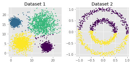
Figure 7: Applying $k$-means algorithm to the two sample datasets.

Figure 8 again shows the datasets $\mathbb{X}^{(1)}$ and $\mathbb{X}^{(2)}$ but with data points clustered using DBSCAN instead of $k$-means. It can be seen that DBSCAN is able to produce reasonable clustering on both datasets and also identifies potential outliers.

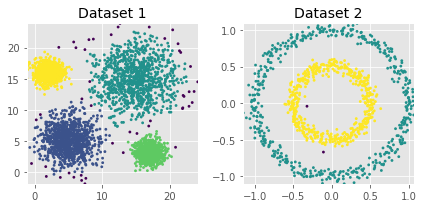
Figure 8: Applying DBSCAN algorithm to the two sample datasets.

References

- [1] A. Krizhevsky, I. Sutskever, and G. Hinton, “Imagenet classification with deep convolutional neural networks,” in Neural Information Processing Systems, NIPS, 2012.
- [2] A. V. Oppenheim, R. W. Schafer, and J. R. Buck, Discrete-Time Signal Processing, 2nd ed. Englewood Cliffs, NJ: Prentice Hall, 1998.
- [3] D. Tse and P. Viswanath, Fundamentals of Wireless Communication. Cambridge University Press, 2005.
- [4] I. Goodfellow, Y. Bengio, and A. Courville, Deep Learning. MIT Press, 2016.
- [5] T. Mikolov, I. Sutskever, K. Chen, G. Corrado, and J. Dean, “Distributed representations of words and phrases and their compositionality,” in Neural Information Processing Systems, NIPS, 2013.
- [6] R. Gray, J. Kieffer, and Y. Linde, “Locally optimal block quantizer design,” Information and Control, vol. 45, pp. 178 – 198, 1980.
- [7] A. Lapidoth, A Foundation in Digital Communication. New York: Cambridge University Press, 2009.
- [8] S. M. Kay, Fundamentals of Statistical Signal Processing: Estimation Theory. Englewood Cliffs, NJ: Prentice Hall, 1993.
- [9] E. L. Lehmann and G. Casella, Theory of Point Estimation, 2nd ed. New York: Springer, 1998.
- [10] C. M. Bishop, Pattern Recognition and Machine Learning. Springer, 2006.
- [11] T. Hastie, R. Tibshirani, and J. Friedman, The Elements of Statistical Learning, ser. Springer Series in Statistics. New York, NY, USA: Springer, 2001.
- [12] L. Xu and M. Jordan, “On convergence properties of the EM algorithm for Gaussian mixtures,” Neural Computation, vol. 8, no. 1, pp. 129–151, 1996.
- [13] M. Ester, H.-P. Kriegel, J. Sander, and X. Xu, “A density-based algorithm for discovering clusters a density-based algorithm for discovering clusters in large spatial databases with noise,” in Proceedings of the Second International Conference on Knowledge Discovery and Data Mining, Portland, Oregon, 1996, pp. 226–231.