Spin transport in disordered long-range interacting spin chain

Abstract

Using a numerically exact technique we study spin transport and the growth of an entanglement profiles in a disordered spin-chain with long-range interactions, decaying as a power-law, $r^{-\alpha}$ with distance and $1.75\leq\alpha\leq 3.25$. Our study confirms the prediction of recent theories that the system is delocalized in this parameters regime. Moreover we find that for $\alpha>3/2$ the entanglement growth is sublinear and the underlying transport is subdiffusive with a transient super-diffusive tail. We show that an appropriately generalized Griffiths picture shows diffusive transport and therefore does not capture the essential properties of the exact dynamics.

Introduction.—Many-body localization (MBL) extends the notion of Anderson localization to interacting systems (Anderson, 1958). For local interactions, its existence is well established theoretically (Basko et al., 2006; Gornyi et al., 2005) and experimentally in one-dimensional systems (Schreiber et al., 2015; Bordia et al., 2016; Smith et al., 2016) (see (Abanin and Papić, 2017) for a recent review), but there is evidence of localization also in two-dimensional systems (Bar Lev and Reichman, 2016; Inglis and Pollet, 2016; Choi et al., 2016; Bordia et al., 2017; Kennes, 2018; Geißler and Pupillo, 2019). For long-range interactions the fate of MBL is less clear. Some studies suggest that the many-body localization is stable for $\alpha>2d$ (Burin, 2006; Yao et al., 2014; Gornyi et al., 2017; Tikhonov and Mirlin, 2018; Nag and Garg, 2019a), some suggest it is stable for $\alpha>d/2$ (Roy and Logan, 2019). Finite size systems of size $L$ are claimed to exhibit an effective many-body-like localization transition at a critical disorder, which for $\alpha<2d$, scales like a power-law with the system size, and therefore diverges in the thermodynamic limit (Burin, 2006, 2015; Gornyi et al., 2017; Tikhonov and Mirlin, 2018; Gopalakrishnan and Huse, 2019). Some theories argue that delocalization occurs also for $\alpha>2d$ though with a critical disorder strength scales which increases slower than algebraically with system size (De Roeck and Huveneers, 2017; Tikhonov and Mirlin, 2018; Gopalakrishnan and Huse, 2019). Understanding the dynamics of disordered systems with long-range interactions is of great importance to a number of physical systems, such as nuclear spins (Alvarez et al., 2015), dipole-dipole interactions of vibrational modes (Levitov, 1989, 1990; Aleiner et al., 2011), Frenkel excitons (Agranovich, 2008), nitrogen vacancy centers in diamond (Childress et al., 2006; Balasubramanian et al., 2009; Neumann et al., 2010; Weber et al., 2010; Dolde et al., 2013) and polarons (Alexandrov and Mott, 1996). Long range interactions are also common in atomic and molecular systems, where interactions can be dipolar (Saffman et al., 2010; Aikawa et al., 2012; Lu et al., 2012; Yan et al., 2013; Gunter et al., 2013; de Paz et al., 2013), van der Waals like (Saffman et al., 2010; Schauß et al., 2012), or even of variable range (Britton et al., 2012; Islam et al., 2013; Richerme et al., 2014; Jurcevic et al., 2014). Some aspects of the dynamics in such systems were studied numerically in Ref. (Safavi-Naini et al., 2019; Nag and Garg, 2019b; Thomson and Schiró, 2020), analytically in Ref.  (Gutman et al., 2016) and experimentally in Ref. Choi et al., 2019, however spin transport in such systems was not considered.

The delocalized phase of one-dimensional systems with local interactions, shows subdiffusive transport (Bar Lev and Reichman, 2014; Bar Lev et al., 2015; Agarwal et al., 2015; Luitz et al., 2016; Žnidarič et al., 2016), accompanied by sublinear growth of the entanglement entropy (Luitz and Bar Lev, 2017; Lezama et al., 2019; Lezama and Luitz, 2019) and intermediate statistics of eigenvalue spacing (Serbyn and Moore, 2016). Anomalous transport is commonly explained by rare insulating regions, which effectively suppress transport in one-dimensional systems. This mechanism is known as the Griffith’s picture (Agarwal et al., 2015; Gopalakrishnan et al., 2015, 2016) (see Ref. (Agarwal et al., 2017) for a recent review and also Ref. (De Roeck et al., 2019) were rare regions were introduced externally). In dimensions higher than one the Griffiths picture predicts diffusion, since rare regions can be circumvented (Gopalakrishnan et al., 2016), however approximate numerical studies (Bar Lev and Reichman, 2016) as also recent experiments (Choi et al., 2016; Bordia et al., 2017) suggest that at least for short to intermediate times the relaxation and transport appear to be anomalous. It is crucial to understand if this discrepancy follows from incompleteness of the Griffiths picture or the approximation of the method. While there are no efficient numerically exact methods to study the dynamics of two-dimensional interacting systems, some progress can be obtained for one-dimensional long-range interacting systems. The Griffiths picture was not generalized to this setting, but in analogy to the reasoning of higher dimensions (Gopalakrishnan et al., 2016), normal diffusive behavior is expected.

In a previous work we have shown that for clean systems with long-range interactions the local part of the Hamiltonian dictates the spreading of the bulk of a local spin excitation, while the long-range part of the Hamiltonian only introduces a weak perturbative effect, in the face of power-law tails of the excitation profile, with an exponent proportional to $\alpha$ (Kloss and Bar Lev, 2019). The tails yield a superdiffusive signature of transport for all $\alpha$, if a sufficiently high moment of the excitation profile is considered (Kloss and Bar Lev, 2019). A natural question which arises is whether the effect of long-range interactions in disordered systems goes beyond a perturbative correction as it happens for their clean counterparts. Moreover, if localization is destabilized by long-range interactions, what is the resulting nature of spin transport?

In this work we consider and answer these questions using a numerically exact matrix product state (MPS) method. The study of long-ranged interacting systems naturally requires large system sizes. In fact, we show that for $\alpha=1.75$, finite size effects are pronounced even for a chain of 51 spins, which is currently considered as the state-of-the-art limit of exact diagonalization based techniques (Wietek and Läuchli, 2018). MPS techniques are therefore indispensable to obtain numerically exact results for chains with long-range interaction, albeit only up to some finite time. This limitation arises since the required numerical effort scales exponentially with the entanglement entropy of the state, which for generic systems is known to grow linearly with time (Kim and Huse, 2013). We stress that our aim here is not to address the question of stability of the MBL phase in the presence of long-range interactions, but to study the dynamics in the delocalized phase. Moreover, since is it technically hard to distinguish between very slow transport and absence of transport, especially in a limited time-interval, our method is not well suited for such purpose.

Time-evolution of long-ranged systems can be conveniently obtained by the time-dependent variational principle (TDVP) applied to the manifold of MPS (Haegeman et al., 2011, 2013, 2016). It was successfully utilized to study the dynamics of spin chains with local interactions in disordered or quasiperiodic potentials (Doggen et al., 2018; Doggen and Mirlin, 2019). For low bond dimensions and very far from the numerically exact limit this method was proposed as an inexpensive candidate to achieve accurate hydrodynamic description of transport (Leviatan et al., 2017), however it was shown to be unreliable for generic systems (Kloss et al., 2018). In this study, we use TDVP as a numerically exact method, and study the nature of transport in long-range-interacting disordered one-dimensional spin chain. We focus on parameter regimes in which the interaction is sufficiently short-ranged such that the corresponding clean system shows asymptotic diffusive behavior, and disorder ranges for which the system is argued to be delocalized by all existing theories.

Model.— We study transport properties of the one-dimensional long-ranged disordered Heisenberg model,

$$\hat{H}=J\sum_{i=1}^{L-1}\sum_{j>i}^{L}\frac{1}{\left(j-i\right){}^{\alpha}}\left(\hat{S}_{i}^{x}\hat{S}_{j}^{x}+\hat{S}_{i}^{y}\hat{S}_{j}^{y}+\hat{S}_{i}^{z}\hat{S}_{j}^{z}\right)+\sum_{i=1}^{L}h_{i}\hat{S}_{i}^{z},$$ (1)

where $h_{i}$ is uniformly distributed in the interval $\left[-W,W\right]$ and $\hat{S}_{i}^{\left(x,y,z\right)}$ are the appropriate projections of the spin-$1/2$ operators on site $i$. In the following, we use $J=1$, which sets the time unit of the problem. To study the dynamical properties of this model we start the system from a random product state, $\left|n\right\rangle$, in the eigenbasis of $\hat{S}_{i}^{z}$ and calculate the growth of the bipartite entanglement entropy $S\left(t\right)$ as also the spreading of a spin-excitation as a function of time, which is assessed from the two-point spin correlation function,

$$C_{x}^{n}(t)=\left\langle n\left|\hat{S}_{L/2+x}^{z}\left(t\right)\hat{S}_{L/2}^{z}\left(0\right)\right|n\right\rangle.$$ (2)

Entanglement entropy is directly available since we use the two-site TDVP method (Haegeman et al., 2016). We then average both $S\left(t\right)$ and $C_{x}^{n}\left(t\right)$, by randomly sampling both the disorder and the initial state of the system, such that any state has an equal probability to occur. This corresponds to infinite temperature ensemble, $C_{x}\left(t\right)=\mathcal{N}^{-1}\sum C_{x}^{n}\left(t\right)$, where $\mathcal{N}$ is the Hilbert space dimension. It is convenient to characterize the spreading by the width of the averaged excitation profile,

$$\sigma^{2}\left(t\right)=\sum_{x=-L/2}^{L/2}x{}^{2}C_{x}\left(t\right)$$ (3)

which is analogous to the classical mean-square displacement (MSD). Typically the MSD scales as, $\sigma^{2}(t)\sim t^{\gamma}$, with $\gamma=2$ ($\gamma=1$) for ballistic (diffusive) transport and $0<\gamma<1$ corresponding to subdiffusive transport. We use the log-derivate to define a time-dependent dynamical exponent $\gamma\left(t\right)=\mathrm{d}\ln\sigma^{2}\left(t\right)/\mathrm{d}\ln t$, which asymptotically converges to $\gamma.$ We similarly define the time-dependent dynamical exponent $\delta\left(t\right)=\mathrm{d}\ln S\left(t\right)/\mathrm{d}\ln t$, to characterize the spread of the entanglement.

Method.— The Hilbert-space dimension of a quantum lattice systems scales exponentially with the size of the system. Any wavefunction in the Hilbert space can be written as a matrix product state (MPS),

$$\left|\Psi[A]\right\rangle=\sum_{\{s_{n}\}=1}^{d}A^{s_{1}}(1)A^{s_{2}}(2)\dots A^{s_{N}}(L)\left|s_{1}s_{2}\dots s_{L}\right\rangle$$ (4)

where $d$ is the local Hilbert space dimension, $A^{s_{i}}(i)\in\mathbb{C}^{D_{i-1}\times D_{i}}$ are complex matrices and $D_{0}=D_{L}=1$, such that the product of matrices evaluates to a scalar coefficient for a given configuration $\left|s_{1}s_{2}\dots s_{L}\right\rangle$. To be an exact representation of the wavefunction the dimension of the matrices, the bond dimension, must scale exponentially with the systems size. Typically one approximates the wavefunction by truncating the dimension of the matrices to a predetermined dimension with computationally tractable number of parameters. Exact results are obtained when the approximate dynamics are converged with respect to the bond dimension.

The time-dependent variational principle (TDVP) allows one to obtain a locally optimal (in time) evolution of the wavefunction on the manifold of MPS, $\mathcal{M}_{\chi},$ with some fixed bond dimension $\chi$. It amounts to solving a tangent-space projected Schrödinger equation (Haegeman et al., 2016):

$$\frac{d\left|\Psi[A]\right\rangle}{dt}=-\mathrm{i}P_{\mathcal{M}}\hat{H}\left|\Psi[A]\right\rangle,$$ (5)

where $P_{\mathcal{M}}$ is the tangent space projector to the manifold $\mathcal{M}_{\chi}$. Equation (5) is solved using a second-order Trotter-Suzuki decomposition of the projector. The Hamiltonian is approximated as a sum of exponentials, which can be efficiently represented as an MPO (Crosswhite et al., 2008). The number of exponentials is chosen such that the resulting couplings do not differ by more than 2% from the exact couplings for any pair of sites. Through this work we have used a bond-dimension of up to $\chi=1024$ and timestep of $dt=0.1$ and verified that our results are convergent with respect to these numerical parameters (see (Sup, )). We average over initial conditions and disorder realizations at the same time and use 1000 realizations unless stated otherwise. All calculations are performed using the TenPy library using a two-site version of the TDVP for MPS and exploiting that the Hamiltonian conserves the total magnetization (Hauschild and Pollmann, 2018), which allows us to directly access to the growth of the entanglement entropy.

Results.—

Figure 1: Rescaled magnetization profiles at different times on log-log scale for bond dimension $\chi=512$ and different disorder strengths ($W=2.0,4.0$ and $6.0$ from left to right). The shaded area shows the standard deviation of the profile obtained from a bootstrapping procedure. Profiles are smoothed by a Gaussian filter with a standard deviation of $2.0$. Black dotted line is a guide to the eye of a power-law, $x^{-2\alpha}$.

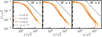
For transport that is not purely diffusive, the MSD contains only partial information on transport, since in this case the asymptotic shape of the profile is not described by a Gaussian. To get a full picture of transport it is therefore pertinent to examine the evolution in time of the excitation profiles, which we do in Fig. 1. Similarly to the clean case in Refs. Kloss and Bar Lev, 2019; Schuckert et al., 2019, the tails of the excitation profile follow a power-law of $-2\alpha$ regardless of the disorder strength, which shows that the disorder cannot suppress the long-range hops of the spin. These tails are responsible for the divergence of the MSD with system size for $\alpha<3/2$. The failure of the rescaling procedure performed in Fig. 1, which is expected to yield a perfect collapse for diffusive transport (c.f. Fig. 5), indicates that transport is not diffusive.

To assess the influence of the disorder on the dynamics we focus on $\alpha=1.75$ and compute the averaged bipartite entanglement and the MSD (3) for a number of disorder strength $W\in\left[2,12\right],$which are predicted to be in the delocalized phase(Tikhonov and Mirlin, 2018)].

Figure 2: Right column. MSD (top panel) and entanglement entropy $S(t)$ (bottom panel) on log-log scale after numerical filtering (see main text) as a function of time for different disorder strengths ($W=2-12$) and $\chi=512$. Left column. $\gamma\left(t\right)$ and $D\left(t\right)$ computed from filtered MSD data, smoothed with a moving average of width $t=4$ (two upper panels), and similarly $\delta\left(t\right)$ and $dS/dt$ computed from filtered $S\left(t\right)$.

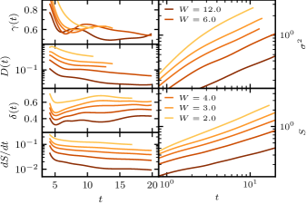
Figure 2 shows the MSD (3) and the entanglement entropy, $S(t)$, as a function of time for various disorder strengths together with the corresponding linear and logarithmic derivatives. All data is converged with respect to the system size ($L=75)$ except for the weakest disorder strength $\left(W=2\right)$ (see (Sup, )). At strong disorder, oscillatory features emerge, with a period of the order of the hopping rate. These oscillations are common in disordered systems, and typically correspond to oscillations between nearby localization centers. Such oscillations hinder to reliably extract the dynamical exponent. In order to rectify this issue we filter-out the corresponding frequency in the Fourier domain (for raw data and a description of the procedure see (Sup, )). As can be seen from Fig. 2 the linear derivatives of MSD and $S\left(t\right)$ are monotonically decreasing with time, while their log-derivatives appear to converge to a constant value smaller than 1. This observation points towards a sub-linear dependence of MSD and $S\left(t\right)$, which is indicative of subdiffusive transport.

Figure 3: Similar to Fig. 3, but for $W=3.0$ and $2.0\leq\alpha\leq 3.25$. System sizes are $L=75$ for $\alpha\leq 2.5$, $L=51$ for $\alpha>2.5$ and $L=35$ for local interactions.

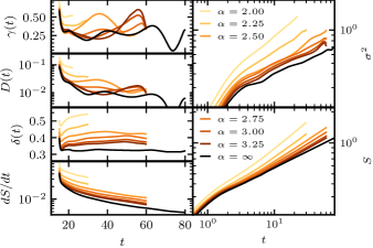
In Fig. 3 we examine the dependence of the dynamics on the range of the interaction by fixing the disorder strength $\left(W=3.0\right)$ and varying $2.0\leq\alpha\leq 3.25$. The disorder is chosen, such that in the local limit, $\alpha\to\infty$ (black line in Fig. 3), the system is delocalized and subdiffusive (Bar Lev et al., 2015). Similarly to Fig. 3, the dynamical exponents $\gamma$ and $\delta$ converge to a constant value smaller than 1 for all studied $\alpha$’s, which is monotonically decreasing with $\alpha$.

Figure 4: Dynamical exponent $1/z$ for MSD (orange hues) and $S(t)$ (blue hues) as a function of $\alpha$ for $W=3.0$ (left panel) and as a function of $W$ for $\alpha=1.75$ (right panel). The exponents and the error bars are obtained as average and standard deviation of the filtered data for the MSD and $S\left(t\right)$ over different windows $\left[t_{S},2^{-\frac{1}{4}}t^{*}\right]$ for left panel and $\left[t_{S},t^{*}\right]$ for right panel, where $t^{*}$ is the time up to which data is converged.

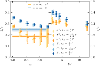
In Fig. 4 we plot the dynamical exponents as extracted from Figs. 2, 3 for different $W$s and $\alpha$’s. We use the relation between the exponents proposed in Refs. (Vosk et al., 2015; Potter et al., 2015) (see also Ref. (Luitz and Bar Lev, 2016)), $1/z=\gamma/2=\delta/\left(1+\delta\right)$ . While the relation is not satisfied well, the overall dependence of the exponents appear similar, with both exponents monotonically decreasing with $\alpha$ and converging to the $\alpha\to\infty$ limit. For $S\left(t\right)$ the dynamical exponent is reliable in the entire range of parameters, but the oscillations in the MSD result in large error bars for $\alpha>2.5$.

Since the exact numerical study of long-range systems is rather limited in time, it is beneficial to find a phenomenological model which attempts to reproduce the relevant dynamical features, and at the same time suggests an effective mechanism. For disordered local systems the Griffiths picture serves this purpose (Agarwal et al., 2015; Gopalakrishnan et al., 2015, 2016). We generalize the Griffiths picture to long-range systems by introducing a finite probability for long jumps with a rate which decays as, $x^{-2\alpha}$, in accord with the long-range part of the Hamiltonian . This reduces to the following master equation,

$$\frac{\partial P_{n}}{\partial t} =\sum_{i}W_{in}P_{i}-\left(\sum_{j}W_{nj}\right)P_{n}$$ (6)

$$W_{ij} =\frac{\mathrm{e}^{-h_{ij}}}{\left|i-j\right|^{2\alpha}}\qquad i\neq j$$

where $h_{ij}$ is a symmetric matrix composed of independent random variables, which stand for the heights of the barriers. The precise shape of the distribution of the barrier heights is not important, as long as it is unbounded, guaranteeing the existence of very weak links. To be concrete, we take it to be the exponential distribution, $p\left(h\right)=h_{0}^{-1}\exp\left[-h/h_{0}\right]$. We note in passing, that while the form of the transition matrix is similar to the power-law random banded matrices used to study Anderson localization with power-law hopping (Mirlin et al., 1996), there are crucial differences: (a) we are applying it to a classical problem, (b) $W_{ij}$ has many-elements close to zero, and must satisfy, $W_{ii}=-\sum_{i\neq j}W_{ij}$. Since long-hops effectively avoid weak-links, such model is expected to be diffusive, but it is important to see how it approaches diffusion as a function of time. To examine that, we numerically solve (6) for about 500 realizations of the transitions rate matrix, $W_{ij}$, with $h_{0}=8$ and a lattice size of $L=1000$. At time $t=0$ the walker is initiated at the origin, $P_{n}\left(t=0\right)=\delta_{n0}$. The probability to find a walker at site $n$ for various times has a Gaussian form in the bulk, followed by a power-law tail, which can be better seen after the rescaling, $\sqrt{t}P_{n}\left(n/\sqrt{t}\right)$ (see Fig. 5). Thus transport in this model is asymptotically diffusive. In Fig. 5 we show the $D\left(t\right)$ and $\gamma\left(t\right)$ for this generalized Griffiths model as a function of time. We note that while $\gamma\left(t\right)$ converges to 1 and $D\left(t\right)$ converges to a constant, indicative of diffusive transport the convergence is quite slow.

Figure 5: Right panel. A rescaled log-log plot of $P_{n}(t)$ for $\alpha=2.0$, $h_{0}=8$ at various times $t$, computed from the solution of the generalized Griffiths model (6). Left panels. The corresponding dynamical exponent $\gamma\left(t\right)$ (top panel) and $D(t)$ (bottom panel).

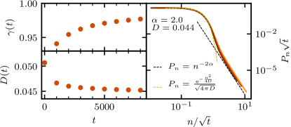
Discussion.—Using a numerically exact method we studied transport in a disordered spin-chain with interactions between the spins decaying as $x^{-\alpha}$ with distance. For clean systems and $\alpha>d/2$ the long-range interaction appears to be a perturbative effect which is manifested by power-law tails of the relevant excitation profile, while the dynamics of the bulk of the excitation is governed by the local interactions (Kloss and Bar Lev, 2019; Luitz and Bar Lev, 2019). Carrying over this analysis to long-range disordered systems suggests localization for sufficiently strong disorder, since local interacting systems exhibit MBL. On the other hand, most studies argue that the addition of long-range interactions is not perturbative, and leads to destruction of localization due to a prevalence of resonances (Burin, 2006; Yao et al., 2014; Gornyi et al., 2017; Tikhonov and Mirlin, 2018). Our study shows that in accord with these works even in the presence of the strongest disorder the system is delocalized. The long-range part of the Hamiltonian thus destabilizes localization and leads to spreading of spin excitations. Our results are consistent with subdiffusive transport, which can be seen in a sub-linear growth of the bipartite entanglement and the MSD. As with any numerical result, our analysis is based on finite times data, therefore we cannot rule out slow drift towards diffusion which might occur for times inaccessible to numerically exact studies. Our findings are not consistent with the prediction for finite heat conductivity, $\kappa\sim W^{-3},$which can be obtained from Ref. (Gutman et al., 2016) for the heat conductivity by setting $\alpha=1.75$ and the temperature to $T=W$. Furthermore, we find that the scaling of the critical disorder strength with system size, advocated by existing theories, does not affect transport in the delocalized phase, at least far away from the critical point. The observed subdiffusive transport is also not consistent with a generalization of the Griffiths mechanism (Gopalakrishnan et al., 2016), which predicts diffusion for long-range systems, since long-range interactions introduce an effective way to circumvent blocking regions. We have confirmed this by a numerical solution of a long-range random-barrier model (6). While in this model, the convergence of the diffusion coefficient to its asymptotic value is quite slow, unlike the long-range model (1), the dynamical exponent is very close to 1, already for short-times, and doesn’t exhibit any plateau for all times. This finding adds up to the mounting evidence against the importance of bottle-necks for subdiffusion, as was shown already in Refs. (Bar Lev and Reichman, 2016; Bar Lev et al., 2017) (cf. (Žnidarič and Ljubotina, 2018; Varma and Žnidarič, 2019), and see also the very recent (Schulz et al., 2019)), suggesting that our understanding of the mechanism of anomalous transport in the vicinity of the MBL transition is far from being complete.

.1 Supplementary material

Figure 6: Convergence of the MSD and $S\left(t\right)$ with respect to the bond dimension at $\alpha=1.75$ for various disorder strengths $W$. Upper panel: MSD and $S\left(t\right)$ at reference bond dimensions $\chi=1024$ ($W=2$ and 3, solid) and $\chi=512$ ($W=4,6$ and 12 solid) and half the reference bond dimension (dashed). Lower panel: Relative errors $\Delta\sigma^{2}$(left panel) and $\Delta S$ (right) between calculations at the reference and half the reference bond dimension. The system size for all panels is $L=75$ and a time-step of $dt=0.1$ was used.

Figure 7: Convergence of the MSD and $S\left(t\right)$ with respect to bond dimension for various $\alpha$ and a disorder strength of $W=3.0$. Upper panel: MSD and $S\left(t\right)$ at bond dimensions $\chi=512$ (solid) and $\chi=256$ (dashed). Lower panel: Relative deviation $\Delta\sigma^{2}$ (left panel) and $\Delta S$ (right) of calculations with $\chi=256$ and $\chi=512$.. The system sizes for all panels are $L=75$ for $\alpha\leq 2.5$, $L=51$ for $2.5<\alpha\leq 3.25$ and $L=35$ for $\alpha=\infty$. A time-step of $dt=0.1$ was used.

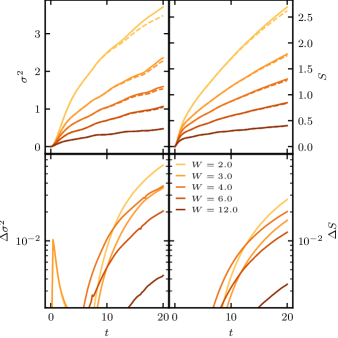
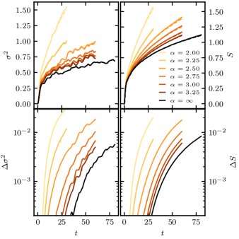
Convergence with respect to numerical parameters.—Numerical exactness of the dynamics generated by TDVP-MPS is obtained by converging with respect to the bond-dimension, $\chi$, as well as the time-step, $dt$. In Fig. 6 , we provide comparisons of the mean-square displacement (MSD) and the entanglement entropy $S(t)$ from calculations with bond-dimensions up to $\chi=1024$. All results for the MSD and $S(t)$ reported in the main article are converged up to a deviation of 2 % between the two largest bond dimensions. In order to check for convergence with the time-step it is sufficient to use a smaller bond dimension, since time-step errors are usually more severe at smaller bond dimension.

Figure 8: Convergence of the MSD with respect to time-step. Relative error $\Delta\sigma^{2}$ compared to a reference calculation with time-step $dt=0.005$ for $L=51$, $\chi=64$ at weak and strong disorder.

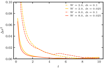
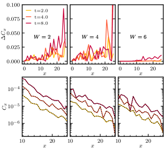
Fig. 8 shows the relative deviation of the MSD at several time-steps from a reference calculation at time-step $dt=0.005$. The large relative error initially is caused by an approximately constant error in absolute terms and that becomes negligible in relative terms after times larger than a few units of the hopping. A time-step of $dt=0.1$ is thus sufficient to obtain a converged MSD within the range of disorder strengths studied. Evaluating the spatial spin excitation profile in the tails at strong disorder becomes sensitive to numerical noise for small values of the correlation function, $C_{x}$, and is limited by a complex interplay of time-step errors and accumulation of numerical round-off errors. As shown in Fig. 9, the convergence of the tails of the spin excitation profile with respect to bond dimension is generally well controlled ($<5\%)$ up to times for which the MSD is converged as well.

Figure 9: Convergence of the spin excitation profiles with respect to bond dimension for $L=51$ and $dt=0.1$ at various disorder strengths and times. Upper panels: Relative error $\Delta C_{x}$ between calculations with $\chi=512$ and $\chi=256$. Lower panels: Tails of spin excitation profiles with $\chi=512$ (solid lines) and $\chi=256$ (black dotted lines).

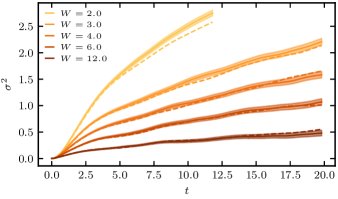
Finite size effects.—In Fig. 10 we provide evidence that the MSD is converged with respect to system size for $L=75$ for the data presented in the main article at $\alpha=1.75$ for all but the smallest disorder strengths $W=2.0$.

Figure 10: Comparison of the MSD for various disorder strengths at $\alpha=1.75$ for system sizes $L=75$ (solid lines) and $L=51$ (dashed lines). The shaded area indicates the standard deviation for $L=75$ obtained from bootstrap sampling.

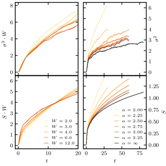
Filtering out high-frequency oscillations.—The presence of strong disorder leads to high frequency oscillations which average only slowly and are an obstacle in analyzing transport properties quantitatively. Hence, we smooth our data by removing the high frequency oscillations according to the following protocol. The linear time derivative of the data is Fourier transformed and a Gaussian broadening is applied in the Fourier domain before transforming back to the time domain, from which the filtered data is obtained by integration. We find that applying a weak broadening at low frequencies, and successively increasing the strength of the broadening at higher frequencies results in an efficient and unbiased removal of the high frequency oscillations. First a broadening of width $w=0.25$ is applied to the range of all nonzero frequencies, followed by a broadening of width $w=0.75$ excluding the two lowest frequencies, and finally a broadening of width $w=1.5$ applied to all but the 4 lowest frequencies. We note that the result depends weakly on the exact values of these parameters. This processing does not result in a systematic bias compared to the raw data, as shown in Fig. 11. The smoothing becomes inefficient towards the boundaries of the support of the data in the time-domain. When available, the raw data has been used past its convergence time as an input for the filtering to circumvent this problem. In the main text, we report only the filtered data and only up to the convergence time determined from Figs. 6 and 7. While this can in principle introduce a bias for the filtering at late times, we verified that the filtered data is consistent with the raw data for all converged times.

Figure 11: Comparison of filtered (solid lines) and unfiltered (dashed lines) MSD (upper panels) and entanglement entropy $S\left(t\right)$ (lower panels) for various disorder strengths at $\alpha=1.75$ (left panels) and for various $\alpha$ with a disorder strength of $W=3.0$ (right panels). For improved visibility, the data for $\alpha=1.75$ (left panels) is rescaled with the disorder strength.

References

- Anderson (1958) P. W. Anderson, Phys. Rev. 109, 1492 (1958)
- Basko et al. (2006) D. Basko, I. L. Aleiner, and B. L. Altshuler, Ann. Phys. (N. Y). 321, 1126 (2006)
- Gornyi et al. (2005) I. V. Gornyi, A. Mirlin, and D. Polyakov, Phys. Rev. Lett. 95, 206603 (2005)
- Schreiber et al. (2015) M. Schreiber, S. S. Hodgman, P. Bordia, H. P. Luschen, M. H. Fischer, R. Vosk, E. Altman, U. Schneider, and I. Bloch, Science (80-. ). 349, 842 (2015)
- Bordia et al. (2016) P. Bordia, H. P. Lüschen, S. S. Hodgman, M. Schreiber, I. Bloch, and U. Schneider, Phys. Rev. Lett. 116, 140401 (2016)
- Smith et al. (2016) J. Smith, A. Lee, P. Richerme, B. Neyenhuis, P. W. Hess, P. Hauke, M. Heyl, D. A. Huse, and C. Monroe, Nat. Phys. 12, 907 (2016)
- Abanin and Papić (2017) D. A. Abanin and Z. Papić, Ann. Phys. 529, 1700169 (2017)
- Bar Lev and Reichman (2016) Y. Bar Lev and D. R. Reichman, EPL (Europhysics Lett. 113, 46001 (2016)
- Inglis and Pollet (2016) S. Inglis and L. Pollet, Phys. Rev. Lett. 117, 120402 (2016), arXiv:1604.07056
- Choi et al. (2016) J.-Y. Choi, S. Hild, J. Zeiher, P. Schauss, A. Rubio-Abadal, T. Yefsah, V. Khemani, D. A. Huse, I. Bloch, and C. Gross, Science (80-. ). 352, 1547 (2016)
- Bordia et al. (2017) P. Bordia, H. Lüschen, S. Scherg, S. Gopalakrishnan, M. Knap, U. Schneider, and I. Bloch, Phys. Rev. X 7, 041047 (2017)
- Kennes (2018) D. M. Kennes, “Many-Body Localization in Two Dimensions from Projected Entangled-Pair States,” (2018), arXiv:1811.04126
- Geißler and Pupillo (2019) A. Geißler and G. Pupillo, “Many-body localization in the two dimensional Bose-Hubbard model,” (2019), arXiv:1909.09247
- Burin (2006) A. L. Burin, (2006), arXiv:0611387 [cond-mat]
- Yao et al. (2014) N. Y. Yao, C. R. Laumann, S. Gopalakrishnan, M. Knap, M. Müller, E. A. Demler, and M. D. Lukin, Phys. Rev. Lett. 113, 243002 (2014)
- Gornyi et al. (2017) I. V. Gornyi, A. D. Mirlin, D. G. Polyakov, and A. L. Burin, Ann. Phys. 529, 1600360 (2017)
- Tikhonov and Mirlin (2018) K. S. Tikhonov and A. D. Mirlin, Phys. Rev. B 97, 214205 (2018)
- Nag and Garg (2019a) S. Nag and A. Garg, Phys. Rev. B 99, 224203 (2019a), arXiv:1903.07354
- Roy and Logan (2019) S. Roy and D. E. Logan, SciPost Phys. 7, 042 (2019)
- Burin (2015) A. L. Burin, Phys. Rev. B 91, 094202 (2015)
- Gopalakrishnan and Huse (2019) S. Gopalakrishnan and D. A. Huse, Phys. Rev. B 99, 134305 (2019)
- De Roeck and Huveneers (2017) W. De Roeck and F. Huveneers, Phys. Rev. B 95, 155129 (2017)
- Alvarez et al. (2015) G. A. Alvarez, D. Suter, and R. Kaiser, Science (80-. ). 349, 846 (2015)
- Levitov (1989) L. S. Levitov, Europhys. Lett. 9, 83 (1989)
- Levitov (1990) L. S. Levitov, Phys. Rev. Lett. 64, 547 (1990)
- Aleiner et al. (2011) I. L. Aleiner, B. L. Altshuler, and K. B. Efetov, Phys. Rev. Lett. 107, 076401 (2011)
- Agranovich (2008) V. Agranovich, Excitations in Organic Solids (Oxford University Press, 2008)
- Childress et al. (2006) L. Childress, M. V. Gurudev Dutt, J. M. Taylor, A. S. Zibrov, F. Jelezko, J. Wrachtrup, P. R. Hemmer, and M. D. Lukin, Science (80-. ). 314, 281 (2006)
- Balasubramanian et al. (2009) G. Balasubramanian, P. Neumann, D. Twitchen, M. Markham, R. Kolesov, N. Mizuochi, J. Isoya, J. Achard, J. Beck, J. Tissler, V. Jacques, P. R. Hemmer, F. Jelezko, and J. Wrachtrup, Nat. Mater. 8, 383 (2009)
- Neumann et al. (2010) P. Neumann, R. Kolesov, B. Naydenov, J. Beck, F. Rempp, M. Steiner, V. Jacques, G. Balasubramanian, M. L. Markham, D. J. Twitchen, S. Pezzagna, J. Meijer, J. Twamley, F. Jelezko, and J. Wrachtrup, Nat. Phys. 6, 249 (2010)
- Weber et al. (2010) J. R. Weber, W. F. Koehl, J. B. Varley, A. Janotti, B. B. Buckley, C. G. Van de Walle, and D. D. Awschalom, Proc. Natl. Acad. Sci. 107, 8513 (2010)
- Dolde et al. (2013) F. Dolde, I. Jakobi, B. Naydenov, N. Zhao, S. Pezzagna, C. Trautmann, J. Meijer, P. Neumann, F. Jelezko, and J. Wrachtrup, Nat. Phys. 9, 139 (2013)
- Alexandrov and Mott (1996) A. S. Alexandrov and N. F. Mott, Polarons and Bipolarons (World Scientific, 1996)
- Saffman et al. (2010) M. Saffman, T. G. Walker, and K. Mølmer, Rev. Mod. Phys. 82, 2313 (2010)
- Aikawa et al. (2012) K. Aikawa, A. Frisch, M. Mark, S. Baier, A. Rietzler, R. Grimm, and F. Ferlaino, Phys. Rev. Lett. 108, 210401 (2012)
- Lu et al. (2012) M. Lu, N. Q. Burdick, and B. L. Lev, Phys. Rev. Lett. 108, 215301 (2012)
- Yan et al. (2013) B. Yan, S. A. Moses, B. Gadway, J. P. Covey, K. R. A. Hazzard, A. M. Rey, D. S. Jin, and J. Ye, Nature 501, 521 (2013)
- Gunter et al. (2013) G. Gunter, H. Schempp, M. Robert-de Saint-Vincent, V. Gavryusev, S. Helmrich, C. S. Hofmann, S. Whitlock, and M. Weidemuller, Science (80-. ). 342, 954 (2013)
- de Paz et al. (2013) A. de Paz, A. Sharma, A. Chotia, E. Maréchal, J. H. Huckans, P. Pedri, L. Santos, O. Gorceix, L. Vernac, and B. Laburthe-Tolra, Phys. Rev. Lett. 111, 185305 (2013)
- Schauß et al. (2012) P. Schauß, M. Cheneau, M. Endres, T. Fukuhara, S. Hild, A. Omran, T. Pohl, C. Gross, S. Kuhr, and I. Bloch, Nature 491, 87 (2012)
- Britton et al. (2012) J. W. Britton, B. C. Sawyer, A. C. Keith, C.-C. J. Wang, J. K. Freericks, H. Uys, M. J. Biercuk, and J. J. Bollinger, Nature 484, 489 (2012)
- Islam et al. (2013) R. Islam, C. Senko, W. C. Campbell, S. Korenblit, J. Smith, A. Lee, E. E. Edwards, C.-C. J. Wang, J. K. Freericks, and C. Monroe, Science (80-. ). 340, 583 (2013)
- Richerme et al. (2014) P. Richerme, Z.-X. Gong, A. Lee, C. Senko, J. Smith, M. Foss-Feig, S. Michalakis, A. V. Gorshkov, and C. Monroe, Nature 511, 198 (2014)
- Jurcevic et al. (2014) P. Jurcevic, B. P. Lanyon, P. Hauke, C. Hempel, P. Zoller, R. Blatt, and C. F. Roos, Nature 511, 202 (2014)
- Safavi-Naini et al. (2019) A. Safavi-Naini, M. L. Wall, O. L. Acevedo, A. M. Rey, and R. M. Nandkishore, Phys. Rev. A 99, 033610 (2019)
- Nag and Garg (2019b) S. Nag and A. Garg, Phys. Rev. B 99, 224203 (2019b)
- Thomson and Schiró (2020) S. J. Thomson and M. Schiró, “Localisation of interacting power-law random banded fermions,” (2020), arXiv:2004.11844 [cond-mat.dis-nn]
- Gutman et al. (2016) D. B. Gutman, I. V. Protopopov, A. L. Burin, I. V. Gornyi, R. A. Santos, and A. D. Mirlin, Phys. Rev. B 93, 245427 (2016)
- Choi et al. (2019) J. Choi, H. Zhou, S. Choi, R. Landig, W. W. Ho, J. Isoya, F. Jelezko, S. Onoda, H. Sumiya, D. A. Abanin, and M. D. Lukin, Phys. Rev. Lett. 122, 043603 (2019)
- Bar Lev and Reichman (2014) Y. Bar Lev and D. R. Reichman, Phys. Rev. B 89, 220201 (2014)
- Bar Lev et al. (2015) Y. Bar Lev, G. Cohen, and D. R. Reichman, Phys. Rev. Lett. 114, 100601 (2015)
- Agarwal et al. (2015) K. Agarwal, S. Gopalakrishnan, M. Knap, M. Müller, and E. Demler, Phys. Rev. Lett. 114, 160401 (2015)
- Luitz et al. (2016) D. J. Luitz, N. Laflorencie, and F. Alet, Phys. Rev. B 93, 060201 (2016)
- Žnidarič et al. (2016) M. Žnidarič, A. Scardicchio, and V. K. Varma, Phys. Rev. Lett. 117, 040601 (2016)
- Luitz and Bar Lev (2017) D. J. Luitz and Y. Bar Lev, Phys. Rev. B 96, 020406 (2017)
- Lezama et al. (2019) T. L. M. Lezama, S. Bera, and J. H. Bardarson, Phys. Rev. B 99, 161106 (2019)
- Lezama and Luitz (2019) T. L. M. Lezama and D. J. Luitz, (2019), arXiv:1908.07010
- Serbyn and Moore (2016) M. Serbyn and J. E. Moore, Phys. Rev. B 93, 041424 (2016)
- Gopalakrishnan et al. (2015) S. Gopalakrishnan, M. Müller, V. Khemani, M. Knap, E. A. Demler, and D. A. Huse, Phys. Rev. B 92, 104202 (2015)
- Gopalakrishnan et al. (2016) S. Gopalakrishnan, K. Agarwal, E. A. Demler, D. A. Huse, and M. Knap, Phys. Rev. B 93, 134206 (2016)
- Agarwal et al. (2017) K. Agarwal, E. Altman, E. Demler, S. Gopalakrishnan, D. A. Huse, and M. Knap, Ann. Phys. 529, 1600326 (2017)
- De Roeck et al. (2019) W. De Roeck, F. Huveneers, and S. Olla, “Subdiffusion in one-dimensional Hamiltonian chains with sparse interactions,” (2019), arXiv:1909.07322
- Kloss and Bar Lev (2019) B. Kloss and Y. Bar Lev, Phys. Rev. A 99, 032114 (2019)
- Wietek and Läuchli (2018) A. Wietek and A. M. Läuchli, Phys. Rev. E 98, 033309 (2018)
- Kim and Huse (2013) H. Kim and D. A. Huse, Phys. Rev. Lett. 111, 127205 (2013)
- Haegeman et al. (2011) J. Haegeman, J. I. Cirac, T. J. Osborne, I. Pižorn, H. Verschelde, and F. Verstraete, Phys. Rev. Lett. 107, 070601 (2011)
- Haegeman et al. (2013) J. Haegeman, T. J. Osborne, and F. Verstraete, Phys. Rev. B 88, 075133 (2013)
- Haegeman et al. (2016) J. Haegeman, C. Lubich, I. Oseledets, B. Vandereycken, and F. Verstraete, Phys. Rev. B 94, 165116 (2016)
- Doggen et al. (2018) E. V. H. Doggen, F. Schindler, K. S. Tikhonov, A. D. Mirlin, T. Neupert, D. G. Polyakov, and I. V. Gornyi, Phys. Rev. B 98, 174202 (2018)
- Doggen and Mirlin (2019) E. V. H. Doggen and A. D. Mirlin, Phys. Rev. B 100, 104203 (2019)
- Leviatan et al. (2017) E. Leviatan, F. Pollmann, J. H. Bardarson, and E. Altman, (2017), arXiv:1702.08894
- Kloss et al. (2018) B. Kloss, Y. Bar Lev, and D. Reichman, Phys. Rev. B 97, 024307 (2018)
- Crosswhite et al. (2008) G. M. Crosswhite, A. C. Doherty, and G. Vidal, Phys. Rev. B 78, 035116 (2008)
- (74) “See supplemental material at [URL] for finite size and other numerical convergence analysis,”
- Hauschild and Pollmann (2018) J. Hauschild and F. Pollmann, SciPost Phys. Lect. Notes , 5 (2018)
- Schuckert et al. (2019) A. Schuckert, I. Lovas, and M. Knap, “Non-local emergent hydrodynamics in a long-range quantum spin system,” (2019), arXiv:1909.01351
- Vosk et al. (2015) R. Vosk, D. A. Huse, and E. Altman, Phys. Rev. X 5, 031032 (2015)
- Potter et al. (2015) A. C. Potter, R. Vasseur, and S. A. Parameswaran, Phys. Rev. X 5, 031033 (2015)
- Luitz and Bar Lev (2016) D. J. Luitz and Y. Bar Lev, Ann. Phys. 529, 1600350 (2016)
- Note (1) The factor of 2 stems from the difference between amplitude and probability
- Mirlin et al. (1996) A. D. Mirlin, Y. V. Fyodorov, F.-M. Dittes, J. Quezada, and T. H. Seligman, Phys. Rev. E 54, 3221 (1996)
- Luitz and Bar Lev (2019) D. J. Luitz and Y. Bar Lev, Phys. Rev. A 99, 010105 (2019)
- Bar Lev et al. (2017) Y. Bar Lev, D. M. Kennes, C. Klöckner, D. R. Reichman, and C. Karrasch, EPL (Europhysics Lett. 119, 37003 (2017)
- Žnidarič and Ljubotina (2018) M. Žnidarič and M. Ljubotina, Proc. Natl. Acad. Sci. 115, 4595 (2018)
- Varma and Žnidarič (2019) V. K. Varma and M. Žnidarič, Phys. Rev. B 100, 1 (2019), arXiv:1905.03128
- Schulz et al. (2019) M. Schulz, S. Taylor, A. Scardicchio, and M. Znidaric, “Phenomenology of anomalous transport in disordered one-dimensional systems,” (2019), arXiv:1909.09507