Spin Networks and Cosmic Strings in 3+1 Dimensions

Spin networks, the quantum states of discrete geometry in loop quantum gravity, are directed graphs whose links are labeled by irreducible representations of SU(2), or spins. Cosmic strings are 1-dimensional topological defects carrying distributional curvature in an otherwise flat spacetime. In this paper we prove that the classical phase space of spin networks coupled to cosmic strings may obtained as a straightforward discretization of general relativity in 3+1 spacetime dimensions. We decompose the continuous spatial geometry into 3-dimensional cells, which are dual to a spin network graph in a unique and well-defined way. Assuming that the geometry may only be probed by holonomies (or Wilson loops) located on the spin network, we truncate the geometry such that the cells become flat and the curvature is concentrated at the edges of the cells, which we then interpret as a network of cosmic strings. The discrete phase space thus describes a spin network coupled to cosmic strings. This work proves that the relation between gravity and spin networks exists not only at the quantum level, but already at the classical level. Two appendices provide detailed derivations of the Ashtekar formulation of gravity as a Yang-Mills theory and the distributional geometry of cosmic strings in this formulation.

1 Introduction

1.1 Loop Quantum Gravity and Spin Networks

When perturbatively quantizing gravity, one obtains a low-energy effective theory, which breaks down at high energies. There are several different approaches to solving this problem and obtaining a theory of quantum gravity. String theory, for example, attempts to do so by postulating entirely new degrees of freedom, which can then be shown to reduce to general relativity (or some modification thereof) at the low-energy limit. Loop quantum gravity [1] instead tries to quantize gravity non-perturbatively, by quantizing holonomies (or Wilson loops) instead of the metric, in an attempt to avoid the issues arising from perturbative quantization.

The starting point of the canonical version of loop quantum gravity [2], which is the one we will discuss here, is the reformulation of general relativity as a non-abelian Yang-Mills gauge theory on a 3-dimensional spatial slice of a 3+1-dimensional spacetime, with the gauge group $\mathrm{SU}\left(2\right)$ related to spatial rotations, the Yang-Mills connection $\mathbf{A}$ related to the usual connection and extrinsic curvature, and the “electric field” $\mathbf{E}$ related to the metric (or more precisely, the frame field). Spatial and time diffeomorphisms appear as additional gauge symmetries, generated by the appropriate constraints. Once gravity is reformulated in this way, one can utilize the existing arsenal of techniques from Yang-Mills theory, and in particular lattice gauge theory, to tackle the problem of quantum gravity [3].

This theory is quantized by considering graphs, that is, sets of nodes connected by links. One defines holonomies, or path-ordered exponentials of the connection, which implement parallel transport along each link. The curvature on the spatial slice can then be probed by looking at holonomies along loops on the graph. Without going into the technical details, the general idea is that if we know the curvature inside every possible loop, then this is equivalent to knowing the curvature at every point.

The kinematical Hilbert space of loop quantum gravity is obtained from the set of all wave-functionals for all possible graphs, together with an appropriate $\mathrm{SU}\left(2\right)$-invariant and diffeomorphism-invariant inner product. The physical Hilbert space is a subset of the kinematical one, containing only the states invariant under all gauge transformations – or in other words, annihilated by all of the constraints. Since gravity is a totally constrained system – in the Hamiltonian formulation, the action is just a sum of constraints – a quantum state annihilated by all of the constraints is analogous to a metric which solves Einstein’s equations in the classical Lagrangian formulation.

Specifically, to get from the kinematical to the physical Hilbert space, three steps must be taken:

1. First, we apply the Gauss constraint to the kinematical Hilbert space. Since the Gauss constraint generates $\mathrm{SU}\left(2\right)$ gauge transformation, we obtain a space of $\mathrm{SU}\left(2\right)$-invariant states, called spin network states [4], which are the graphs mentioned above, but with their links colored by irreducible representations of $\mathrm{SU}\left(2\right)$, that is, spins $j\in\left\{\frac{1}{2},1,\frac{3}{2},2,\ldots\right\}$.

2. Then, we apply the spatial diffeomorphism constraint. We obtain a space of equivalence classes of spin networks under spatial diffeomorphisms, a.k.a. knots. These states are now abstract graphs, not localized in space. This is analogous to how a classical geometry is an equivalence class of metrics under diffeomorphisms.

3. Lastly, we apply the Hamiltonian constraint. This step is still not entirely well-understood, and is one of the main open problems of the theory.

One of loop quantum gravity’s most celebrated results is the existence of area and volume operators. They are derived by taking the usual integrals of area and volume forms and promoting the “electric field” $\mathbf{E}$, which is conjugate to the connection $\mathbf{A}$, to a functional derivative $\delta/\delta\mathbf{A}$. The spin network states turn out to be eigenstates of these operators, and they have discrete spectra which depend on the spins of the links. This means that loop quantum gravity contains a quantum geometry, which is a feature one would expect a quantum theory of spacetime to have. It also hints that spacetime is discrete at the Planck scale.

However, it is not clear how to rigorously define the classical geometry related to a particular spin network state. In this paper, we will try to answer that question. In our previous two papers [5, 6] we showed how to obtain the phase space of spin networks coupled to point particles by discretizing gravity in 2+1D; this paper generalizes that result to 3+1D.

1.2 Quantization, Discretization, Subdivision, and Truncation

One of the key challenges in trying to define a theory of quantum gravity at the quantum level is to find a regularization that does not drastically break the fundamental symmetries of the theory. This is a challenge in any gauge theory, but gravity is especially challenging, for two reasons. First, one expects that the quantum theory possesses a fundamental length scale; and second, the gauge group contains diffeomorphism symmetry, which affects the nature of the space on which the regularization is applied.

In gauge theories such as quantum chromodynamics (QCD), the only known way to satisfy these requirements, other than gauge-fixing before regularization, is to put the theory on a lattice, where an effective finite-dimensional gauge symmetry survives at each scale. One would like to devise such a scheme in the gravitational context as well. In this paper, we develop a step-by-step procedure to achieve this, exploiting, among other things, the fact that first-order gravity in 3+1 dimensions with the Ashtekar variables closely resembles other gauge theories, as discussed above. We find not only the spin network (or holonomy-flux) phase space, but also additional string-like degrees of freedom coupled to the curvature and torsion.

As explained above, in canonical loop quantum gravity, one can show that the geometric operators possess a discrete spectrum. This is, however, only possible after one chooses the quantum spin network states to have support on a graph. Spin network states can be understood as describing a quantum version of discretized spatial geometry [1], and the Hilbert space associated to a graph can be related, in the classical limit, to a set of discrete piecewise-flat geometries [7, 8].

This means that the loop quantum gravity quantization scheme consists at the same time of a quantization and a discretization; moreover, the quantization of the geometric spectrum is entangled with the discretization of the fundamental variables. It has been argued that it is essential to disentangle these two different features [9], especially when one wants to address dynamical issues.

In [9, 10], it was suggested that one should understand the discretization as a two-step process: a subdivision followed by a truncation. In the first step one subdivides the systems into fundamental cells, and in the second step one chooses a truncation of degrees of freedom in each cell, which is consistent with the symmetries of the theory. By focusing first on the classical discretization, before any quantization takes place, several aspects of the theory can be clarified, as we discussed in [5].

The separation of discretization into two distinct steps in our formalism work as follows. First we perform a subdivision, or decomposition into subsystems. More precisely, we define a cellular decomposition on our 3D spatial manifold, where the cells can be any (convex) polyhedra. This structure has a dual structure, which as we will see, is the spin network graph, with each cell dual to a node, and each side dual to a link connected to that node.

Then, we perform a truncation, or coarse-graining of the subsystems. In this step, we assume that there is arbitrary curvature and torsion inside each loop of the spin network. We then “compress” the information about the geometry into singular codimension-2 excitations, which is 3 spatial dimensions means 1-dimensional (string) excitation. Crucially, since the only way to probe the geometry is by looking at the holonomies on the loops of the spin network, the observables before and after this truncation are the same.

Another way to interpret this step is to instead assume that spacetime is flat everywhere, with matter sources being distributive, i.e., given by Dirac delta functions, which then generate singular curvature and torsion by virtue of the Einstein equation. We interpret these distributive matter sources as strings, and this is entirely equivalent to truncating a continuous geometry, since holonomies cannot distinguish between continuous and distributive geometries.

Once we performed subdivision and truncation, we can now define discrete variables on each cell and integrate the continuous symplectic potential in order to obtain a discrete potential, which represents the discrete phase space. In this step, we will see that the mathematical structures we are using conspire to cancel many terms in the potential, allowing us to fully integrate it.

1.3 Outline

This paper is organized as follows. First, in Chapter 2, we provide a comprehensive list of basic definitions, notations, and conventions which will be used throughout the paper. It is recommended that the reader not skip this chapter, as some of our notation is slightly non-standard.

In Chapter 3 and Appendix A we provide a detailed and self-contained derivation of the Ashtekar variables and the loop gravity Hamiltonian action, including the constraints. Special care is taken to write everything in terms of index-free Lie-algebra-valued differential forms, which – in addition to being more elegant – will greatly simplify our derivation.

Chapter 4 introduces the cellular decomposition and explains how an arbitrary geometry is truncated into a piecewise-flat geometry, or alternatively, a flat geometry with matter degrees of freedom in the form of cosmic strings. Appendix B discusses cosmic strings in detail, and derives their representation in the Ashtekar formulation. Chapter 5 presents the classical spin network phase space, and provides a detailed calculation of the Poisson brackets.

Chapter 6 is the main part of the paper, where we will use the structures and results of the previous chapters to obtain the spin network phase space coupled to cosmic strings from the continuous phase space of 3+1-dimensional gravity. Finally, Chapter 7 summarizes the results of this paper and presents several avenues for potential future research.

The content of this paper, together with that of our previous two papers [5, 6], may also be found in the author’s PhD thesis [11]. The thesis relates and compares the 2+1D and 3+1D calculations, adds a simpler way to perform the 2+1D calculation which did not appear in the previous papers, includes an extensive discussion of the role of edge modes in our formalism, and contains much more detailed derivations of some results.

2 Basic Definitions, Notations, and Conventions

The following definitions, notations, and conventions will be used throughout the paper.

2.1 Lie Group and Algebra Elements

Let $G$ be a Lie group, let $\mathfrak{g}$ be its associated Lie algebra, and let $\mathfrak{g}^{*}$ be the dual to that Lie algebra. The cotangent bundle of $G$ is the Lie group $T^{*}G\cong G\ltimes\mathfrak{g}^{*}$, where $\ltimes$ is the semidirect product, and it has the associated Lie algebra $\mathfrak{g}\oplus\mathfrak{g}^{*}$. We assume that this group is the Euclidean group, or a generalization thereof, and its algebra takes the form

$$\left[\mathbf{P}_{i},\mathbf{P}_{j}\right]=0,\qquad\left[\mathbf{J}_{i},\mathbf{J}_{j}\right]=f_{ij}{}^{k}\mathbf{J}_{k},\qquad\left[\mathbf{J}_{i},\mathbf{P}_{j}\right]=f_{ij}{}^{k}\mathbf{P}_{k},$$ (2.1)

where:

• $f_{ij}{}^{k}$ are the structure constants, which satisfy anti-symmetry $f_{ij}{}^{k}=-f_{ji}{}^{k}$ and the Jacobi identity $f_{[ij}{}^{l}f_{k]l}{}^{m}=0$.

• $\mathbf{J}_{i}\in\mathfrak{g}$ are the rotation generators,

• $\mathbf{P}_{i}\in\mathfrak{g}^{*}$ are the translation generators,

• The indices $i,j,k$ take the values $1,2,3$, since they are internal spatial indices.

Note that sometimes we will use the notation $\boldsymbol{\tau}_{i}$ to indicate generators which could be in either $\mathfrak{g}$ or $\mathfrak{g}^{*}$.

Usually in the loop quantum gravity literature we take $G=\mathrm{SU}\left(2\right)$ such that $\mathfrak{g}^{*}=\mathbb{R}^{3}$ and

$$\mathrm{ISU}\left(2\right)\cong\mathrm{SU}\left(2\right)\ltimes\mathbb{R}^{3}\cong T^{*}\mathrm{SU}\left(2\right).$$ (2.2)

However, here we will keep $G$ abstract for brevity and in order for the discussion to be more general.

Throughout this paper, different fonts and typefaces will distinguish elements of different groups and algebras, or differential forms valued in those groups and algebras, as follows:

• $G\ltimes\mathfrak{g}^{*}$-valued forms will be written in Calligraphic font: $\mathcal{A},\mathcal{B},\mathcal{C},...$

• $\mathfrak{g}\oplus\mathfrak{g}^{*}$-valued forms will be written in bold Calligraphic font: $\boldsymbol{\mathcal{A}},\boldsymbol{\mathcal{B}},\boldsymbol{\mathcal{C}},...$

• $G$-valued forms will be written in regular font: $a,b,c,...$

• $\mathfrak{g}$ or $\mathfrak{g}^{*}$-valued forms will be written in bold font: $\mathbf{a},\mathbf{b},\mathbf{c},...$

The Calligraphic notation will only be used in this introduction; elsewhere we will only talk about $G$, $\mathfrak{g}$, or $\mathfrak{g}^{*}$ elements.

2.2 Indices and Differential Forms

Throughout this paper, we will use the following conventions for indices:

• $\mu,\nu,\ldots\in\left\{0,1,2,3\right\}$ represent 3+1D spacetime components.

• $A,B,\ldots,I,J,\ldots\in\left(0,1,2,3\right)$ represent 3+1D internal components.

• $a,b,\ldots\in\left\{1,2,3\right\}$ represent 3D spatial components: $\overbrace{0,\underbrace{1,2,3}_{a}}^{\mu}$.

• $i,j,\ldots\in\left\{1,2,3\right\}$ represent 3D internal / Lie algebra components: $\overbrace{0,\underbrace{1,2,3}_{i}}^{I}$.

We consider a 3+1D manifold $M$ with topology $\Sigma\times\mathbb{R}$ where $\Sigma$ is a 3-dimensional spatial manifold and $\mathbb{R}$ represents time. Our metric signature convention is $\left(-,+,+,+\right)$. In index-free notation, we denote a Lie-algebra-valued differential form of degree $p$ (or $p$-form) on $\Sigma$, with one algebra index $i$ and $p$ spatial indices $a_{1},\ldots,a_{p}$, as

$$\mathbf{A}\equiv\frac{1}{p!}A_{a_{1}\cdots a_{p}}^{i}\boldsymbol{\tau}_{i}\thinspace\mathrm{d}x^{a_{1}}\wedge\cdots\wedge\mathrm{d}x^{a_{p}}\in\Omega^{p}\left(\Sigma,\mathfrak{g}\right),$$ (2.3)

where $A_{a_{1}\cdots a_{p}}^{i}$ are the components and $\boldsymbol{\tau}_{i}$ are the generators of the algebra $\mathfrak{g}$ in which the form is valued.

Sometimes we will only care about the algebra index, and write $\mathbf{A}\equiv A^{i}\boldsymbol{\tau}_{i}$ with the spatial indices implied, such that $A^{i}\equiv\frac{1}{p!}A_{a_{1}\cdots a_{p}}^{i}\mathrm{d}x^{a_{1}}\wedge\cdots\wedge\mathrm{d}x^{a_{p}}$ are real-valued $p$-forms. Other times we will only care about the spacetime indices, and write $\mathbf{A}\equiv\frac{1}{p!}\mathbf{A}_{a_{1}\cdots a_{p}}\mathrm{d}x^{a_{1}}\wedge\cdots\wedge\mathrm{d}x^{a_{p}}$ with the algebra index implied, such that $\mathbf{A}_{a_{1}\cdots a_{p}}\equiv A_{a_{1}\cdots a_{p}}^{i}\boldsymbol{\tau}_{i}$ are algebra-valued 0-forms.

2.3 The Graded Commutator

Given any two Lie-algebra-valued forms $\mathbf{A}$ and $\mathbf{B}$ of degrees $\deg\mathbf{A}$ and $\deg\mathbf{B}$ respectively, we define the graded commutator:

$$\left[\mathbf{A},\mathbf{B}\right]\equiv\mathbf{A}\wedge\mathbf{B}-\left(-1\right)^{\deg\mathbf{A}\deg\mathbf{B}}\mathbf{B}\wedge\mathbf{A},$$ (2.4)

which satisfies

$$\left[\mathbf{A},\mathbf{B}\right]=-\left(-1\right)^{\deg\mathbf{A}\deg\mathbf{B}}\left[\mathbf{B},\mathbf{A}\right].$$ (2.5)

If at least one of the forms has even degree, this reduces to the usual anti-symmetric commutator; if we then interpret $\mathbf{A}$ and $\mathbf{B}$ as vectors in $\mathbb{R}^{3}$, then this is none other than the vector cross product $\mathbf{A}\times\mathbf{B}$. Note that $\left[\mathbf{A},\mathbf{B}\right]$ is a Lie-algebra-valued $\left(\deg\mathbf{A}+\deg\mathbf{B}\right)$-form.

The graded commutator satisfies the graded Leibniz rule:

$$\mathrm{d}\left[\mathbf{A},\mathbf{B}\right]=\left[\mathrm{d}\mathbf{A},\mathbf{B}\right]+\left(-1\right)^{\deg\mathbf{A}}\left[\mathbf{A},\mathrm{d}\mathbf{B}\right].$$ (2.6)

In terms of indices, with $\deg\mathbf{A}=p$ and $\deg\mathbf{B}=q$, we have

$$\left[\mathbf{A},\mathbf{B}\right]=\frac{1}{\left(p+q\right)!}\left[\mathbf{A},\mathbf{B}\right]_{a_{1}\cdots a_{p}b_{1}\cdots b_{q}}^{k}\boldsymbol{\tau}_{k}\mathrm{d}x^{a_{1}}\wedge\cdots\wedge\mathrm{d}x^{a_{p}}\wedge\mathrm{d}x^{b_{1}}\wedge\cdots\wedge\mathrm{d}x^{b_{q}},$$ (2.7)

where

$$\left[\mathbf{A},\mathbf{B}\right]_{a_{1}\cdots a_{p}b_{1}\cdots b_{q}}^{k}\equiv\frac{\left(p+q\right)!}{p!q!}\epsilon^{k}{}_{ij}A_{[a_{1}\cdots a_{p}}^{i}B_{b_{1}\cdots b_{q}]}^{j}.$$ (2.8)

In terms of spatial indices alone, we have

$$\left[\mathbf{A},\mathbf{B}\right]_{a_{1}\cdots a_{p}b_{1}\cdots b_{q}}\equiv\frac{\left(p+q\right)!}{p!q!}\epsilon^{k}{}_{ij}A_{[a_{1}\cdots a_{p}}^{i}B_{b_{1}\cdots b_{q}]}^{j}\boldsymbol{\tau}_{k},$$ (2.9)

and in terms of Lie algebra indices alone, we simply have

$$\left[\mathbf{A},\mathbf{B}\right]^{k}=\epsilon^{k}{}_{ij}A^{i}B^{j}.$$ (2.10)

2.4 The Graded Dot Product and the Triple Product

We define a dot (inner) product, also known as the Killing form, on the generators of the Lie group as follows:

$$\mathbf{J}_{i}\cdot\mathbf{P}_{j}=\delta_{ij},\qquad\mathbf{J}_{i}\cdot\mathbf{J}_{j}=\mathbf{P}_{i}\cdot\mathbf{P}_{j}=0,$$ (2.11)

where $\delta_{ij}$ is the Kronecker delta. Given two Lie-algebra-valued forms $\mathbf{A}$ and $\mathbf{B}$ of degrees $\deg\mathbf{A}$ and $\deg\mathbf{B}$ respectively, such that $\mathbf{A}\equiv A^{i}\mathbf{J}_{i}$ is a pure rotation and $\mathbf{B}\equiv B^{i}\mathbf{P}_{i}$ is a pure translation, we define the graded dot product:

$$\mathbf{A}\cdot\mathbf{B}\equiv\delta_{ij}A^{i}\wedge B^{j},$$ (2.12)

where $\wedge$ is the usual wedge product of differential forms. The dot product satisfies

$$\mathbf{A}\cdot\mathbf{B}=\left(-1\right)^{\deg\mathbf{A}\deg\mathbf{B}}\mathbf{B}\cdot\mathbf{A}.$$ (2.13)

Again, if at least one of the forms has even degree, this reduces to the usual symmetric dot product. Note that $\mathbf{A}\cdot\mathbf{B}$ is a real-valued $\left(\deg\mathbf{A}+\deg\mathbf{B}\right)$-form.

The graded dot product satisfies the graded Leibniz rule:

$$\mathrm{d}\left(\mathbf{A}\cdot\mathbf{B}\right)=\mathrm{d}\mathbf{A}\cdot\mathbf{B}+\left(-1\right)^{\deg\mathbf{A}}\mathbf{A}\cdot\mathrm{d}\mathbf{B}.$$ (2.14)

In terms of indices, with $\deg\mathbf{A}=p$ and $\deg\mathbf{B}=q$, we have

$$\mathbf{A}\cdot\mathbf{B}=\frac{1}{\left(p+q\right)!}\left(\mathbf{A}\cdot\mathbf{B}\right)_{a_{1}\cdots a_{p}b_{1}\cdots b_{q}}\mathrm{d}x^{a_{1}}\wedge\cdots\wedge\mathrm{d}x^{a_{p}}\wedge\mathrm{d}x^{b_{1}}\wedge\cdots\wedge\mathrm{d}x^{b_{q}},$$ (2.15)

where

$$\left(\mathbf{A}\cdot\mathbf{B}\right)_{a_{1}\cdots a_{p}b_{1}\cdots b_{q}}=\frac{\left(p+q\right)!}{p!q!}\delta_{ij}A_{[a_{1}\cdots a_{p}}^{i}B_{b_{1}\cdots b_{q}]}^{j}.$$ (2.16)

Since the graded dot product is a trace, and thus cyclic, it satisfies

$$\left(g^{-1}\mathbf{A}g\right)\cdot\left(g^{-1}\mathbf{B}g\right)=\mathbf{A}\cdot\mathbf{B},$$ (2.17)

where $g$ is any group element. We will use this identity many times throughout the paper to simplify expressions.

Finally, by combining the dot product and the commutator, we obtain the triple product:

$$\left[\mathbf{A},\mathbf{B}\right]\cdot\mathbf{C}=\mathbf{A}\cdot\left[\mathbf{B},\mathbf{C}\right]=\epsilon_{ijk}A^{i}\wedge B^{j}\wedge C^{k}.$$ (2.18)

Note that this is a real-valued $\left(\deg\mathbf{A}+\deg\mathbf{B}+\deg\mathbf{C}\right)$-form. The triple product inherits the symmetry and anti-symmetry properties of the dot product and the commutator.

2.5 Variational Anti-Derivations on Field Space

In addition to the familiar exterior derivative (or differential) $\mathrm{d}$ and interior product $\iota$ on spacetime, we introduce a variational exterior derivative (or variational differential) $\delta$ and a variational interior product $I$ on field space. These operators act analogously to $\mathrm{d}$ and $\iota$, and in particular they are nilpotent, e.g. $\delta^{2}=0$, and satisfy the graded Leibniz rule as defined above.

Degrees of differential forms are counted with respect to spacetime and field space separately; for example, if $f$ is a 0-form then $\mathrm{d}\delta f$ is a 1-form on spacetime, due to $\mathrm{d}$, and independently also a 1-form on field space, due to $\delta$. The dot product defined above also includes an implicit wedge product with respect to field-space forms, such that e.g. $\delta\mathbf{A}\cdot\delta\mathbf{B}=-\delta\mathbf{B}\cdot\delta\mathbf{A}$ if $\mathbf{f}$ and $\mathbf{g}$ are 0-forms on field space. In this paper, the only place where one should watch out for the wedge product and graded Leibniz rule on field space is when we will discuss the symplectic form, which is a field-space 2-form; everywhere else, we will only deal with field-space 0-forms and 1-forms.

We also define a convenient shorthand notation for the Maurer-Cartan 1-form on field space:

$$\boldsymbol{\Delta}g\equiv\delta gg^{-1},$$ (2.19)

where $g$ is a $G$-valued 0-form, which satisfies

$$\boldsymbol{\Delta}\left(gh\right)=\boldsymbol{\Delta}g+g\boldsymbol{\Delta}hg^{-1}=g\left(\boldsymbol{\Delta}h-\boldsymbol{\Delta}(g^{-1})\right)g^{-1},$$ (2.20)

$$\boldsymbol{\Delta}g^{-1}=-g^{-1}\boldsymbol{\Delta}gg,\qquad\delta\left(\boldsymbol{\Delta}g\right)=\frac{1}{2}\left[\boldsymbol{\Delta}g,\boldsymbol{\Delta}g\right].$$ (2.21)

Note that $\boldsymbol{\Delta}g$ is a $\mathfrak{g}$-valued form; in fact, $\boldsymbol{\Delta}$ can be interpreted as a map from the Lie group $G$ to its Lie algebra $\mathfrak{g}$.

2.6 $G\ltimes\mathfrak{g}^{*}$-valued Holonomies and the Adjacent Subscript Rule

A $G\ltimes\mathfrak{g}^{*}$-valued holonomy from a point $a$ to a point $b$ will be denoted as

$$\mathcal{H}_{ab}\equiv\overrightarrow{\exp}\int_{a}^{b}\boldsymbol{\mathcal{A}},$$ (2.22)

where $\boldsymbol{\mathcal{A}}$ is the $\mathfrak{g}\oplus\mathfrak{g}^{*}$-valued connection 1-form and $\overrightarrow{\exp}$ is a path-ordered exponential. Composition of two holonomies works as follows:

$$\mathcal{H}_{ab}\mathcal{H}_{bc}=\left(\overrightarrow{\exp}\int_{a}^{b}\boldsymbol{\mathcal{A}}\right)\left(\overrightarrow{\exp}\int_{b}^{c}\boldsymbol{\mathcal{A}}\right)=\overrightarrow{\exp}\int_{a}^{c}\boldsymbol{\mathcal{A}}=\mathcal{H}_{ac}.$$ (2.23)

Therefore, in our notation, adjacent holonomy subscripts must always be identical; a term such as $\mathcal{H}_{ab}\mathcal{H}_{cd}$ is illegal, since one can only compose two holonomies if the second starts where the first ends. Inversion of holonomies works as follows:

$$\mathcal{H}_{ab}^{-1}=\left(\overrightarrow{\exp}\int_{a}^{b}\boldsymbol{\mathcal{A}}\right)^{-1}=\overrightarrow{\exp}\int_{b}^{a}\boldsymbol{\mathcal{A}}=\mathcal{H}_{ba}.$$ (2.24)

For the Maurer-Cartan 1-form on field space, we move the end point of the holonomy to a superscript:

$$\boldsymbol{\Delta}\mathcal{H}_{a}^{b}\equiv\delta\mathcal{H}_{ab}\mathcal{H}_{ba}.$$ (2.25)

On the right-hand side, the subscripts $b$ are adjacent, so the two holonomies $\delta\mathcal{H}_{ab}$ and $\mathcal{H}_{ba}$ may be composed. However, one can only compose $\boldsymbol{\Delta}\mathcal{H}_{a}^{b}$ with a holonomy that starts at $a$, and $b$ is raised to a superscript to reflect that. For example, $\boldsymbol{\Delta}\mathcal{H}_{a}^{b}\mathcal{H}_{bc}$ is illegal, since this is actually $\delta\mathcal{H}_{ab}\mathcal{H}_{ba}\mathcal{H}_{bc}$ and the holonomies $\mathcal{H}_{ba}$ and $\mathcal{H}_{bc}$ cannot be composed. However, $\boldsymbol{\Delta}\mathcal{H}_{a}^{b}\mathcal{H}_{ac}$ is perfectly legal, and results in $\delta\mathcal{H}_{ab}\mathcal{H}_{ba}\mathcal{H}_{ac}=\delta\mathcal{H}_{ab}\mathcal{H}_{bc}$.

Note that from (2.20) and (2.21) we have

$$\boldsymbol{\Delta}\mathcal{H}_{b}^{a}=-\mathcal{H}_{ba}\boldsymbol{\Delta}\mathcal{H}_{a}^{b}\mathcal{H}_{ab},$$ (2.26)

$$\boldsymbol{\Delta}\mathcal{H}_{a}^{c}=\boldsymbol{\Delta}\left(\mathcal{H}_{ab}\mathcal{H}_{bc}\right)=\boldsymbol{\Delta}\mathcal{H}_{a}^{b}+\mathcal{H}_{ab}\boldsymbol{\Delta}\mathcal{H}_{b}^{c}\mathcal{H}_{ba}=\mathcal{H}_{ab}\left(\boldsymbol{\Delta}\mathcal{H}_{b}^{c}-\boldsymbol{\Delta}\mathcal{H}_{b}^{a}\right)\mathcal{H}_{ba},$$ (2.27)

both of which are compatible with the adjacent subscripts rule.

2.7 The Cartan Decomposition

We can split a $G\ltimes\mathfrak{g}^{*}$-valued (Euclidean) holonomy $\mathcal{H}_{ab}$ into a rotational holonomy $h_{ab}$, valued in $G$, and a translational holonomy $\mathbf{x}_{a}^{b}$, valued in $\mathfrak{g}^{*}$. We do this using the Cartan decomposition

$$\mathcal{H}_{ab}\equiv\operatorname{e}^{\mathbf{x}_{a}^{b}}h_{ab},\qquad\mathcal{H}_{ab}\in\Omega^{0}\left(\Sigma,G\ltimes\mathfrak{g}^{*}\right),\qquad h_{ab}\in\Omega^{0}\left(\Sigma,G\right),\qquad\mathbf{x}_{a}^{b}\in\Omega^{0}\left(\Sigma,\mathfrak{g}^{*}\right).$$ (2.28)

In the following, we will employ the useful identity

$$h\operatorname{e}^{\mathbf{x}}h^{-1}=\operatorname{e}^{h\mathbf{x}h^{-1}},\qquad h\in\Omega^{0}\left(\Sigma,G\right),\qquad\mathbf{x}\in\Omega^{0}\left(\Sigma,\mathfrak{g}^{*}\right),$$ (2.29)

which for matrix Lie algebras (such as the ones we use here) may be proven by writing the exponential as a power series.

Taking the inverse of $\mathcal{H}_{ab}$ and using (2.29), we get

$$\mathcal{H}_{ab}^{-1}=\left(\operatorname{e}^{\mathbf{x}_{a}^{b}}h_{ab}\right)^{-1}=h_{ab}^{-1}\operatorname{e}^{-\mathbf{x}_{a}^{b}}=h_{ab}^{-1}\operatorname{e}^{-\mathbf{x}_{a}^{b}}\left(h_{ab}h_{ab}^{-1}\right)=\operatorname{e}^{-h_{ab}^{-1}\mathbf{x}_{a}^{b}h_{ab}}h_{ab}^{-1}.$$ (2.30)

But on the other hand

$$\mathcal{H}_{ab}^{-1}=\mathcal{H}_{ba}=\operatorname{e}^{\mathbf{x}_{b}^{a}}h_{ba}.$$ (2.31)

Therefore, we conclude that

$$h_{ba}=h_{ab}^{-1},\qquad\mathbf{x}_{b}^{a}=-h_{ab}^{-1}\mathbf{x}_{a}^{b}h_{ab}.$$ (2.32)

Similarly, composing two $G\ltimes\mathfrak{g}^{*}$-valued holonomies and using (2.29) and (2.32), we get

$$\mathcal{H}_{ab}\mathcal{H}_{bc} =\left(\operatorname{e}^{\mathbf{x}_{a}^{b}}h_{ab}\right)\left(\operatorname{e}^{\mathbf{x}_{b}^{c}}h_{bc}\right)$$

$$=\operatorname{e}^{\mathbf{x}_{a}^{b}}h_{ab}\operatorname{e}^{\mathbf{x}_{b}^{c}}\left(h_{ba}h_{ab}\right)h_{bc}$$

$$=\operatorname{e}^{\mathbf{x}_{a}^{b}}\operatorname{e}^{h_{ab}\mathbf{x}_{b}^{c}h_{ba}}h_{ab}h_{bc}$$

$$=\operatorname{e}^{\mathbf{x}_{a}^{b}+h_{ab}\mathbf{x}_{b}^{c}h_{ba}}h_{ab}h_{bc},$$

where we used the fact that $\mathfrak{g}^{*}$ is abelian, and therefore the exponentials may be combined linearly. On the other hand

$$\mathcal{H}_{ab}\mathcal{H}_{bc}=\mathcal{H}_{ac}=\operatorname{e}^{\mathbf{x}_{a}^{c}}h_{ac},$$ (2.33)

so we conclude that

$$h_{ac}=h_{ab}h_{bc},\qquad\mathbf{x}_{a}^{c}=\mathbf{x}_{a}^{b}\oplus\mathbf{x}_{b}^{c}\equiv\mathbf{x}_{a}^{b}+h_{ab}\mathbf{x}_{b}^{c}h_{ba}=h_{ab}\left(\mathbf{x}_{b}^{c}-\mathbf{x}_{b}^{a}\right)h_{ba},$$ (2.34)

where in the second identity we denoted the composition of the two translational holonomies with a $\oplus$, and used (2.32) to get the right-hand side. It is now clear why the end point of the translational holonomy is a superscript – again, this is for compatibility with the adjacent subscript rule.

3 Gravity as a Gauge Theory in the Ashtekar Formulation

We will now present the action and phase space structure for classical gravity in 3+1 spacetime dimensions, as formulated using the Ashtekar variables. As explained above, this formulation allows us to describe gravity as a Yang-Mills gauge theory. The interested reader may refer to Appendix A and to [11] for a complete and detailed derivation of these results. Here, we just summarize them.

3.1 The Ashtekar Action with Indices

In Appendix A, we find that the Ashtekar action of classical loop gravity is:

$$S=\frac{1}{\gamma}\int\mathrm{d}t\int_{\Sigma}\mathrm{d}^{3}x\left(\tilde{E}_{i}^{a}\partial_{t}A_{a}^{i}+\lambda^{i}G_{i}+N^{a}V_{a}+NC\right),$$ (3.1)

where:

• $\gamma$ is the Barbero-Immirzi parameter,

• $\Sigma$ is a 3-dimensional spatial slice,

• $a,b,c,\ldots\in\left\{1,2,3\right\}$ are spatial indices on $\Sigma$,

• $i,j,k,\ldots\in\left\{1,2,3\right\}$ are indices in the Lie algebra $\mathfrak{g}$,

• $\tilde{E}_{i}^{a}\equiv\det\left(e\right)e_{i}^{a}$ is the densitized triad, a rank $\left(1,0\right)$ tensor of density weight $-1$, where $e_{i}^{a}$ is the inverse frame field (or triad), related to the inverse spatial metric $g^{ab}$ via $g^{ab}=e_{i}^{a}e_{j}^{b}\delta^{ij}$,

• $A_{a}^{i}$ is the Ashtekar-Barbero connection,

• $\partial_{t}$ is the derivative with respect to the time coordinate $t$, such that each spatial slice is at a constant value of $t$,

• $\lambda^{i}$, $N^{a}$ and $N$ are Lagrange multipliers,

• $G_{i}\equiv\partial_{a}\tilde{E}_{i}^{a}+\epsilon_{ij}^{k}A_{a}^{j}\tilde{E}_{k}^{a}$ is the Gauss constraint,

• $V_{a}\equiv\tilde{E}_{i}^{b}F_{ab}^{i}$ is the vector (or momentum or diffeomorphism) constraint, where $F_{ab}^{i}$ is the curvature of the Ashtekar-Barbero connection:

  $$F_{ab}^{i}\equiv\partial_{a}A_{b}^{i}-\partial_{b}A_{a}^{i}+\epsilon_{jk}^{i}A_{a}^{j}A_{b}^{k}.$$ (3.2)

• $C$ is the scalar (or Hamiltonian) constraint, defined as

  $$C\equiv\frac{\epsilon_{i}^{mn}\tilde{E}_{m}^{a}\tilde{E}_{n}^{b}}{2\sqrt{\det\left(\tilde{E}\right)}}\left(F_{ab}^{i}-\left(1+\gamma^{2}\right)\epsilon_{jk}^{i}K_{a}^{j}K_{b}^{k}\right),$$ (3.3)

  where $K_{a}^{i}$ is the extrinsic curvature.

From the first term in the action, we see that the connection and densitized triad are conjugate variables, and they form the Poisson algebra

$$\left\{A_{a}^{i}\left(x\right),A_{b}^{j}\left(y\right)\right\}=\left\{\tilde{E}_{i}^{a}\left(x\right),\tilde{E}_{j}^{b}\left(y\right)\right\}=0,$$ (3.4)

$$\left\{A_{a}^{i}\left(x\right),\tilde{E}_{j}^{b}\left(y\right)\right\}=\gamma\delta_{j}^{i}\delta_{a}^{b}\delta\left(x,y\right).$$ (3.5)

3.2 The Ashtekar Action in Index-Free Notation

In index-free notation, which we will use throughout this paper, the action takes the form

$$S=\frac{1}{\gamma}\int\mathrm{d}t\int_{\Sigma}\left(\mathbf{E}\cdot\partial_{t}\mathbf{A}+\boldsymbol{\lambda}\cdot\left[\mathbf{e},\mathbf{P}\right]+\mathbf{N}\cdot\left[\mathbf{e},\mathbf{F}\right]+N\left(\mathbf{e}\cdot\mathbf{F}-\frac{1}{2}\left(\frac{1}{\gamma}+\gamma\right)\mathbf{K}\cdot\mathbf{P}\right)\right),$$ (3.6)

where now:

• $\mathbf{E}\equiv\frac{1}{2}\left[\mathbf{e},\mathbf{e}\right]$ is the electric field 2-form, defined in terms of the densitized triad and the frame field as

  $$\mathbf{E}\equiv\frac{1}{2}E_{ab}^{i}\boldsymbol{\tau}_{i}\mathrm{d}x^{a}\wedge\mathrm{d}x^{b}\quad\Longrightarrow\quad E_{ab}^{i}=\tilde{\epsilon}_{abc}\delta^{ij}\tilde{E}_{j}^{c}=\epsilon_{jk}^{i}e_{a}^{j}e_{b}^{k}.$$ (3.7)

• $\mathbf{A}\equiv A_{a}^{i}\boldsymbol{\tau}_{i}\mathrm{d}x^{a}$ is the $\mathfrak{g}$-valued Ashtekar-Barbero connection 1-form.

• $\mathbf{e}\equiv e_{a}^{i}\boldsymbol{\tau}_{i}\mathrm{d}x^{a}$ is the $\mathfrak{g}$-valued frame field 1-form.

• $\mathbf{P}\equiv\mathrm{d}_{\mathbf{A}}\mathbf{e}$ is a $\mathfrak{g}$-valued 2-form.

• The Gauss constraint is $\boldsymbol{\lambda}\cdot\left[\mathbf{e},\mathbf{P}\right]=\boldsymbol{\lambda}\cdot\mathrm{d}_{\mathbf{A}}\mathbf{E}$ where the Lagrange multiplier $\boldsymbol{\lambda}$ is a $\mathfrak{g}$-valued 0-form.

• The vector (or momentum or diffeomorphism) constraint is $\mathbf{N}\cdot\left[\mathbf{e},\mathbf{F}\right]$ where the Lagrange multiplier $\mathbf{N}$ is a $\mathfrak{g}$-valued 0-form and $\mathbf{F}$ is the $\mathfrak{g}$-valued curvature 2-form

  $$\mathbf{F}\equiv\mathrm{d}_{\mathbf{A}}\mathbf{A}\equiv\mathrm{d}\mathbf{A}+\frac{1}{2}\left[\mathbf{A},\mathbf{A}\right].$$ (3.8)

• The scalar (or Hamiltonian) constraint is $N\left(\mathbf{e}\cdot\mathbf{F}-\frac{1}{2}\left(\frac{1}{\gamma}+\gamma\right)\mathbf{K}\cdot\mathbf{P}\right)$ where the Lagrange multiplier $N$ is a 0-form, not valued in $\mathfrak{g}$, and $\mathbf{K}\equiv K_{a}^{i}\boldsymbol{\tau}_{i}\mathrm{d}x^{a}$ is the $\mathfrak{g}$-valued extrinsic curvature 1-form.

Finally, the symplectic potential, in index-free notation, is

$$\Theta=\int_{\Sigma}\mathbf{E}\cdot\delta\mathbf{A},$$ (3.9)

and it corresponds to the symplectic form

$$\Omega\equiv\delta\Theta=\int_{\Sigma}\delta\mathbf{E}\cdot\delta\mathbf{A}.$$ (3.10)

The reader is referred to Appendix A for derivations of the index-free expressions.

3.3 The Constraints as Generators of Symmetries

Let $\mathcal{C}$ be the space of smooth connections on $\Sigma$. The kinematical (unconstrained) phase space of 3+1-dimensional gravity is given by the cotangent bundle $\mathcal{P}\equiv T^{*}\mathcal{C}$. To get the physical (that is, gauge-invariant) phase space, we must perform symplectic reductions with respect to the constraints. These constraints are best understood in their smeared form as generators of gauge transformations. The smeared Gauss constraint can be written as

$$\mathcal{G}\left(\boldsymbol{\alpha}\right)\equiv\frac{1}{2}\int_{\Sigma}\boldsymbol{\lambda}\cdot\mathrm{d}_{\mathbf{A}}\mathbf{E},$$ (3.11)

where $\boldsymbol{\lambda}$ is a $\mathfrak{g}$-valued 0-form. This constraint generates the infinitesimal $G$ gauge transformations:

$$\left\{\mathbf{A},\mathcal{G}\left(\boldsymbol{\lambda}\right)\right\}\propto\mathrm{d}_{\mathbf{A}}\boldsymbol{\lambda},\qquad\left\{\mathbf{E},\mathcal{G}\left(\boldsymbol{\lambda}\right)\right\}\propto\left[\mathbf{E},\boldsymbol{\lambda}\right].$$ (3.12)

The smeared vector constraint is given by

$$\mathcal{V}\left(\xi\right)\equiv\int_{\Sigma}\mathbf{N}\cdot\left[\mathbf{e},\mathbf{F}\right],$$ (3.13)

where $\xi^{a}$ is a spatial vector and the Lagrange multiplier $N^{i}\equiv\xi^{a}e_{a}^{i}$ is a $\mathfrak{g}$-valued 0-form. From the Gauss and vector constraints we may construct the diffeomorphism constraint:

$$\mathcal{D}\left(\xi\right)\equiv\mathcal{V}\left(\xi\right)-\mathcal{G}\left(\xi\lrcorner\thinspace\mathbf{A}\right),$$ (3.14)

where $\xi\lrcorner\thinspace\mathbf{A}\equiv\xi^{a}A_{a}^{i}\boldsymbol{\tau}_{i}$ is an interior product (see Footnote 5). This constraint generates the infinitesimal spatial diffeomorphism transformations

$$\left\{\mathbf{A},\mathcal{D}\left(\xi\right)\right\}\propto\mathcal{L}_{\xi}\mathbf{A},\qquad\left\{\mathbf{E},\mathcal{D}\left(\xi\right)\right\}\propto\mathcal{L}_{\xi}\mathbf{E},$$ (3.15)

where $\mathcal{L}_{\xi}$ is the Lie derivative.

4 The Discrete Geometry

In this chapter, we will present the discrete geometry under consideration: a cellular decomposition, with curvature and torsion located only on the edges of the cells, which we interpret as a network of cosmic strings.

4.1 The Cellular Decomposition and Its Dual

We embed a cellular decomposition $\Delta$ and a dual cellular decomposition $\Delta^{*}$ in our 3-dimensional spatial manifold $\Sigma$. These structures consist of the following elements, where each element of $\Delta$ is uniquely dual to an element of $\Delta^{*}$. Each cell $c\in\Delta$ is uniquely dual to a node $c^{*}\in\Delta^{*}$. The boundary of the cell $c$ is composed of sides $s_{1},s_{2},\ldots\in\Delta$, which are uniquely dual to links $s_{1}^{*},s_{2}^{*},\ldots\in\Delta^{*}$; these links are exactly all the links which are connected to the node $c^{*}$. The boundary of each side is composed of edges $e_{1},e_{2},\ldots\in\Delta$, which are uniquely dual to faces $e_{1}^{*},e_{2}^{*},\ldots\in\Delta^{*}$. Finally, the boundary of each edge is composed of vertices $v,v^{\prime}\in\Delta$, which are uniquely dual to volumes $v^{*},v^{\prime*}\in\Delta^{*}$. This is summarized in the following table:

$\Delta$		$\Delta^{*}$
0-cells (vertices) $v$	dual to	3-cells (volumes) $v^{*}$
1-cells (edges) $e$	dual to	2-cells (faces) $e^{*}$
2-cells (sides) $s$	dual to	1-cells (links) $s^{*}$
3-cells (cells) $c$	dual to	0-cells (nodes) $c^{*}$

We will write:

• $c=\left(s_{1},\ldots,s_{n}\right)$ to indicate that the boundary of the cell $c$ is composed of the $n$ sides $s_{1},\ldots,s_{n}$.

• $s=\left(e_{1},\ldots,e_{n}\right)$ to indicate that the boundary of the side $s$ is composed of the $n$ edges $e_{1},\ldots,e_{n}$.

• $s=\left(cc^{\prime}\right)$ to indicate that the side $s$ is shared by the two cells $c,c^{\prime}$.

• $s^{*}=\left(cc^{\prime}\right)^{*}$ to indicate that the link $s^{*}$ (dual to the side $s$) connects the two nodes $c^{*}$ and $c^{\prime*}$ (dual to the cells $c,c^{\prime}$).

• $e=\left(c_{1},\ldots,c_{n}\right)$ to indicate the the edge $e$ is shared by the $n$ cells $c_{1},\ldots,c_{n}$.

• $e=\left(s_{1},\ldots,s_{n}\right)$ to indicate the the edge $e$ is shared by the $n$ sides $s_{1},\ldots,s_{n}$.

• $e=\left(vv^{\prime}\right)$ to indicate that the edge $e$ connects the two vertices $v,v^{\prime}$.

The 1-skeleton graph $\Gamma\subset\Delta$ is the set of all vertices and edges of $\Delta$. It is dual to the spin network graph $\Gamma^{*}\subset\Delta^{*}$, the set of all nodes and links of $\Delta^{*}$. Both graphs are oriented. This construction is illustrated in Figure 1.

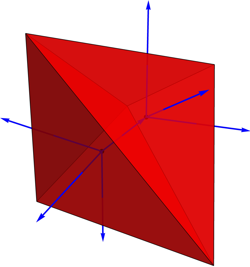
Figure 1: A simple discretization with two cells (in red) and a dual spin network (in blue). Here, the discretization is the simplest possible one: a simplicial complex, where the cells are 3-simplices (tetrahedrons) and their faces are 2-simplices (triangles). The edges are 1-simplices (line segments), and the vertices are, of course, 0-simplices (points). However, our formalism also allows the cells to be arbitrary convex polyhedra and the faces to be arbitrary convex polygons. From the figure, it should be clear that each of the two cells is dual to a node (located inside it), and each of the faces is dual to a link, with the face shared by the two cells dual to the link connecting the two nodes. This is further illustrated by Figure 2.

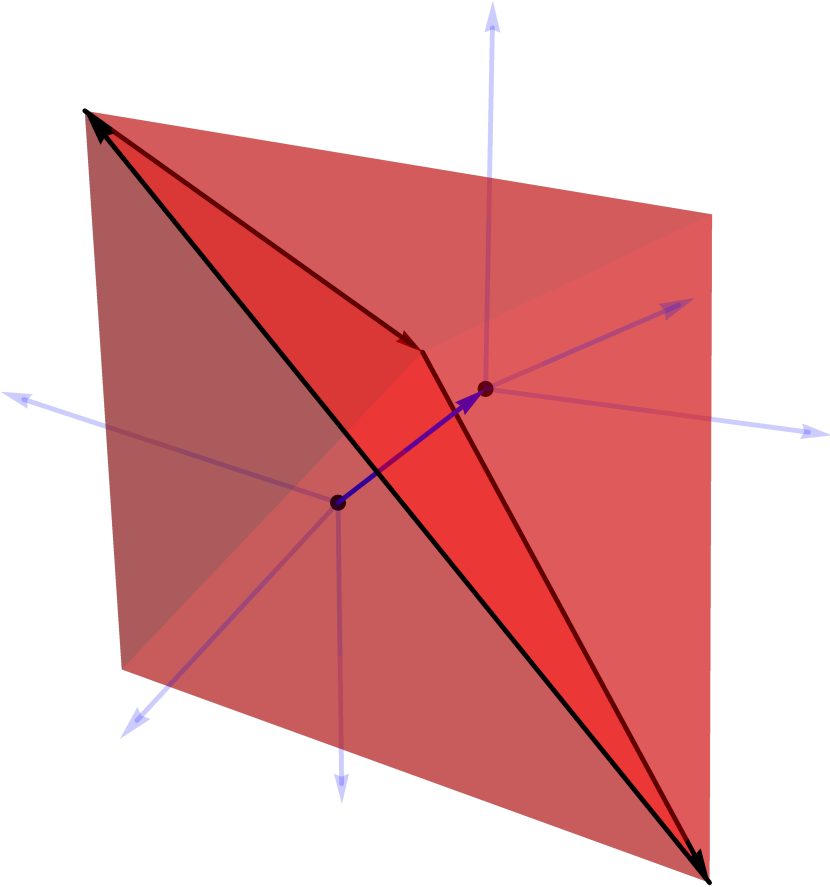
Figure 2: For clarity, we have highlighted the middle link, the two nodes it connects, the (triangular) face shared by the two cells, and the edges on the boundary on that face (which are, as illustrated, oriented) – and dimmed everything else.

4.2 Truncating the Geometry to the Edges

The connection $\mathbf{A}$ and frame field $\mathbf{e}$ inside each cell $c$ – that is, on the interior of the cell, but not on the edges and vertices – are taken to be

$$\mathbf{A}\bigl{|}_{c}=h_{c}^{-1}\mathrm{d}h_{c},\qquad\mathbf{e}\bigl{|}_{c}=h_{c}^{-1}\mathrm{d}\mathbf{x}_{c}h_{c}\quad\Longrightarrow\quad\mathbf{E}\bigl{|}_{c}=\frac{1}{2}\left[\mathbf{e},\mathbf{e}\right]\bigl{|}_{c}=h_{c}^{-1}\left[\mathrm{d}\mathbf{x}_{c},\mathrm{d}\mathbf{x}_{c}\right]h_{c},$$ (4.1)

in analogy with the 2+1D case discussed in [5, 6]. Since they correspond to

$$\mathbf{F}\equiv\mathrm{d}_{\mathbf{A}}\mathbf{A}=0,\qquad\mathbf{P}\equiv\mathrm{d}_{\mathbf{A}}\mathbf{e}=0,$$ (4.2)

they trivially solve all of the constraints:

$$\left[\mathbf{e},\mathbf{P}\right]=\left[\mathbf{e},\mathbf{F}\right]=\mathbf{e}\cdot\mathbf{F}-\frac{1}{2}\left(\frac{1}{\gamma}+\gamma\right)\mathbf{K}\cdot\mathbf{P}=0.$$ (4.3)

We also impose that $\mathbf{F}$ and $\mathbf{P}$ are non-zero only on the edges:

$$\mathbf{F}=\sum_{e}\mathbf{p}_{e}\delta^{\left(2\right)}\left(e\right),\qquad\mathbf{P}=\sum_{e}\mathbf{j}_{e}\delta^{\left(2\right)}\left(e\right),$$ (4.4)

where $\delta^{\left(2\right)}\left(e\right)$ is a delta 2-form such that for any 1-form $f$

$$\int_{\Sigma}f\wedge\delta^{\left(2\right)}\left(e\right)=\int_{e}f,$$ (4.5)

as discussed in Appendix (B), and $\mathbf{p}_{e}$, $\mathbf{j}_{e}$ are constant algebra elements encoding the curvature and torsion on each edge. These distributional curvature and torsion describe a network of cosmic strings: 1-dimensional topological defects carrying curvature and torsion in an otherwise flat spacetime. The expressions (4.4) are derived from first principles in Appendix B.

This construction describes a piecewise-flat-and-torsionless geometry; the cells are flat and torsionless, and the curvature and torsion are located only on the edges of the cells. We may interpret the 1-skeleton $\Gamma$, the set of all edges in the cellular decomposition $\Delta$, as a network of cosmic strings.

The reason for considering this particular geometry comes from the assumption that the geometry can only be probed by taking loops of holonomies along the spin network. Imagine a 3-dimensional slice $\Sigma$ with arbitrary geometry. We first embed a spin network $\Gamma^{*}$, which can be any graph, in $\Sigma$. Then we draw a dual graph, $\Gamma$, such that each edge of $\Gamma$ passes through exactly one loop of $\Gamma^{*}$. We take a holonomy along each of the loops of $\Gamma^{*}$, and encode the result on the edges of $\Gamma$. The resulting discrete geometry is exactly the one we described above, and it is completely equivalent to the continuous geometry with which we started, since the holonomies along the spin network cannot tell the difference between the continuous geometry and the discrete one.

In short, given a choice of a particular spin network, an arbitrary continuous geometry may be reduced to an equivalent discrete geometry, given by a network of cosmic strings, one for each loop of the spin network.

5 Classical Spin Networks

Our goal is to show that, by discretizing the continuous phase space of gravity, we obtain the spin network phase space of loop quantum gravity, coupled to cosmic strings. Therefore, before we perform our discretization, let us study the spin network phase space.

5.1 The Spin Network Phase Space

In the previous chapter, we defined the spin network $\Gamma^{*}$ as a collection of links $e^{*}$ connecting nodes $c^{*}$. The kinematical spin network phase space is isomorphic to a direct product of $T^{*}G$ cotangent bundles for each link $e^{*}\in\Gamma^{*}$:

$$P_{\Gamma^{*}}\equiv\underset{e^{*}\in\Gamma^{*}}{\prod}T^{*}G.$$ (5.1)

Since $T^{*}G\cong G\ltimes\mathfrak{g}^{*}$, the phase space variables are a group element $h_{e^{*}}\in G$ and a Lie algebra element $\mathbf{X}_{e^{*}}\in\mathfrak{g}^{*}$ for each link $e^{*}\in\Gamma^{*}$. Under orientation reversal of the link $e^{*}$ we have, according to (2.32),

$$h_{e^{*-1}}=h_{e^{*}}^{-1},\qquad\mathbf{X}_{e^{*-1}}=-h_{e^{*}}^{-1}\mathbf{X}_{e^{*}}h_{e^{*}}.$$ (5.2)

These variables satisfy the Poisson algebra derived in the next section:

$$\{h_{e^{*}},h_{e^{\prime*}}\}=0,\qquad\{X_{e^{*}}^{i},X_{e^{\prime*}}^{j}\}=\delta_{e^{*}e^{\prime*}}\epsilon^{ij}{}_{k}X_{e^{*}}^{k},\qquad\{X_{e^{*}}^{i},h_{e^{\prime*}}\}=\delta_{e^{*}e^{\prime*}}h_{e^{*}}\mathbf{J}^{i},$$ (5.3)

where $e^{*}$ and $e^{\prime*}$ are two links and $\mathbf{J}^{i}$ are the generators of $\mathfrak{g}$.

The symplectic potential is

$$\Theta=\sum_{e^{*}\in\Gamma^{*}}\boldsymbol{\Delta}h_{e^{*}}\cdot\mathbf{X}_{e^{*}},$$ (5.4)

where we used the graded dot product defined in Section 2.4 and the Maurer-Cartan form defined in (2.19). This phase space enjoys the action of the gauge group $G^{N}$, where $N$ is the number of nodes in $\Gamma^{*}$. This action is generated by the discrete Gauss constraint at each node,

$$\mathbf{G}_{c}\equiv\sum_{e^{*}\ni c^{*}}\mathbf{X}_{e^{*}},$$ (5.5)

where $e^{*}\ni c^{*}$ means “all links $e^{*}$ connected to the node $c^{*}$”. This means that the sum of the fluxes vanishes when summed over all the links connected to the node $c^{*}$. Given a link $e^{*}=\left(cc^{\prime}\right)^{*}$, the action of the Gauss constraint is given in terms of two group elements $g_{c},g_{c^{\prime}}\in G$, one at each node, as

$$h_{e^{*}}\mapsto g_{c}h_{e^{*}}g_{c^{\prime}}^{-1},\qquad\mathbf{X}_{e^{*}}\mapsto g_{c}\mathbf{X}_{e^{*}}g_{c}^{-1}.$$ (5.6)

5.2 Calculation of the Poisson Brackets

Let us calculate the Poisson brackets of the spin network phase space $T^{*}G$, for one link. For the Maurer-Cartan form, we use the notation

$$\boldsymbol{\theta}\equiv-\boldsymbol{\Delta}h\equiv-\delta hh^{-1}.$$ (5.7)

This serves two purposes: first, we can talk about the components $\theta^{i}$ of $\boldsymbol{\theta}$ without the notation getting too cluttered, and second, from (2.21), the Maurer-Cartan form thus defined satisfies the Maurer-Cartan structure equation

$$\mathbf{F}\left(\boldsymbol{\theta}\right)\equiv\delta_{\boldsymbol{\theta}}\boldsymbol{\theta}\equiv\delta\boldsymbol{\theta}+\frac{1}{2}\left[\boldsymbol{\theta},\boldsymbol{\theta}\right]=0,$$ (5.8)

where $\mathbf{F}\left(\boldsymbol{\theta}\right)$ is the curvature of $\boldsymbol{\theta}$. Note that $\boldsymbol{\theta}$ is a $\mathfrak{g}$-valued 1-form on field space, and we also have a $\mathfrak{g}^{*}$-valued 0-form $\mathbf{X}$, the flux. We take a set of vector fields $\mathbf{q}_{i}$ and $\mathbf{p}_{i}$ for $i\in\left\{1,2,3\right\}$ which are chosen to satisfy

$$\mathbf{q}_{j}\lrcorner\thinspace\theta^{i}=\mathbf{p}_{j}\lrcorner\thinspace\delta X^{i}=\delta_{J}^{i},\qquad\mathbf{p}_{j}\lrcorner\thinspace\theta^{i}=\mathbf{q}_{j}\lrcorner\thinspace\delta X^{i}=0,$$ (5.9)

where $\lrcorner\thinspace$ is the usual interior product on differential forms. The symplectic potential on one link is taken to be

$$\Theta=-\boldsymbol{\theta}\cdot\mathbf{X},$$ (5.11)

and its symplectic form is

$$\Omega\equiv\delta\Theta =-\delta\left(\boldsymbol{\theta}\cdot\mathbf{X}\right)=-\left(\delta\boldsymbol{\theta}\cdot\mathbf{X}-\boldsymbol{\theta}\cdot\delta\mathbf{X}\right)$$

$$=-\left(-\frac{1}{2}\left[\boldsymbol{\theta},\boldsymbol{\theta}\right]\cdot\mathbf{X}-\boldsymbol{\theta}\cdot\delta\mathbf{X}\right)$$

$$=\delta\mathbf{X}\cdot\boldsymbol{\theta}+\frac{1}{2}\mathbf{X}\cdot\left[\boldsymbol{\theta},\boldsymbol{\theta}\right],$$

where in the first line we used the graded Leibniz rule (on field-space forms) and in the second line we used (5.8). In components, we have

$$\Omega=\delta X_{k}\wedge\theta^{k}+\frac{1}{2}\epsilon_{ijk}\theta^{i}\wedge\theta^{j}X^{k}.$$ (5.12)

Now, recall the definition of the Hamiltonian vector field of $f$: it is the vector field $\mathbf{H}_{f}$ satisfying

$$\mathbf{H}_{f}\lrcorner\thinspace\Omega=-\delta f.$$ (5.13)

Let us contract the vector field $\mathbf{q}_{i}$ with $\Omega$ using $\mathbf{q}_{j}\lrcorner\thinspace\theta^{i}=\delta_{J}^{i}$ and $\mathbf{q}_{j}\lrcorner\thinspace\delta X^{i}=0$:

$$\mathbf{q}_{l}\lrcorner\thinspace\Omega =\mathbf{q}_{l}\lrcorner\thinspace\left(\delta X_{k}\wedge\theta^{k}+\frac{1}{2}\epsilon_{ijk}\theta^{i}\wedge\theta^{j}X^{k}\right)$$

$$=-\delta X_{k}\delta_{l}^{k}+\frac{1}{2}\epsilon_{ijk}\delta_{l}^{i}\theta^{j}X^{k}-\frac{1}{2}\epsilon_{ijk}\delta_{l}^{j}\theta^{i}X^{k}$$

$$=-\delta X_{l}+\epsilon_{ljk}\theta^{j}X^{k}.$$

Similarly, let us contract $\mathbf{p}_{i}$ with $\Omega$ using $\mathbf{p}_{j}\lrcorner\thinspace\delta X^{i}=\delta_{J}^{i}$ and $\mathbf{p}_{j}\lrcorner\thinspace\theta^{i}=0$:

$$\mathbf{p}_{l}\lrcorner\thinspace\Omega=\mathbf{p}_{l}\lrcorner\thinspace\left(\delta X_{k}\wedge\theta^{k}+\frac{1}{2}\epsilon_{ijk}\theta^{i}\wedge\theta^{j}X^{k}\right)=\delta_{kl}\theta^{k}=\theta_{l}.$$ (5.14)

Note that

$$-\delta X_{i}=\mathbf{q}_{i}\lrcorner\thinspace\Omega-\epsilon_{ijk}\theta^{j}X^{k}=\mathbf{q}_{i}\lrcorner\thinspace\Omega-\epsilon_{ijk}\left(\mathbf{p}^{j}\lrcorner\thinspace\Omega\right)X^{k}.$$ (5.15)

Thus, we can construct the Hamiltonian vector field for $X^{i}$:

$$\mathbf{H}_{X_{i}}\equiv\mathbf{q}_{i}-\epsilon_{ijk}\mathbf{p}^{j}X^{k},\qquad\mathbf{H}_{X_{i}}\lrcorner\thinspace\Omega=-\delta X_{i}.$$ (5.16)

As for $h$, we consider explicitly the matrix components in the fundamental representation, $h_{\ B}^{A}$. The Hamiltonian vector field for the component $h_{\ B}^{A}$ satisfies, by definition,

$$\mathbf{H}_{h_{\ B}^{A}}\lrcorner\thinspace\Omega=-\delta h_{\ B}^{A}.$$ (5.17)

If we multiply by $\left(h^{-1}\right)_{\ C}^{B}$, we get

$$\left(\mathbf{H}_{h_{\ B}^{A}}\left(h^{-1}\right)_{\ C}^{B}\right)\lrcorner\thinspace\Omega=-\delta h_{\ B}^{A}\left(h^{-1}\right)_{\ C}^{B}=\left(-\delta hh^{-1}\right)_{\ C}^{A}=\theta^{i}\left(\mathbf{J}_{i}\right)_{\ C}^{A}=\left(\mathbf{p}^{i}\left(\mathbf{J}_{i}\right)_{\ C}^{A}\right)\lrcorner\thinspace\Omega.$$ (5.18)

Thus we conclude that the Hamiltonian vector field for $h_{\ B}^{A}$ is

$$\mathbf{H}_{h_{\ B}^{A}}=\left(h\mathbf{J}_{i}\right)_{\ B}^{A}\mathbf{p}^{i}.$$ (5.19)

Now that we have found $\mathbf{H}_{X_{i}}$ and $\mathbf{H}_{h_{\ B}^{A}}$, we can finally calculate the Poisson brackets. First, we have

$$\left\{h_{\ B}^{A},h_{\ D}^{C}\right\} =-\Omega\left(\mathbf{H}_{h_{\ B}^{A}},\mathbf{H}_{h_{\ D}^{C}}\right)$$

$$=-\left(\delta X_{k}\wedge\theta^{k}+\frac{1}{2}\epsilon_{ijk}\theta^{i}\wedge\theta^{j}X^{k}\right)\left(\left(h\mathbf{J}_{l}\right)_{\ B}^{A}\mathbf{p}^{l},\left(h\mathbf{J}_{m}\right)_{\ D}^{C}\mathbf{p}^{m}\right)$$

$$=0,$$

since $\mathbf{p}_{j}\lrcorner\thinspace\theta^{i}=0$. Thus

$$\left\{h,h\right\}=0.$$ (5.20)

Next, we have

$$\left\{X^{i},X^{j}\right\} =-\Omega\left(\mathbf{H}_{X^{i}},\mathbf{H}_{X^{j}}\right)$$

$$=-\left(\delta X_{k}\wedge\theta^{k}+\frac{1}{2}\epsilon_{pqk}\theta^{p}\wedge\theta^{q}X^{k}\right)\left(\mathbf{q}^{i}-\epsilon_{lm}^{i}\mathbf{p}^{l}X^{m},\mathbf{q}^{j}-\epsilon_{no}^{j}\mathbf{p}^{n}X^{o}\right)$$

$$=\epsilon_{lm}^{i}\delta_{k}^{l}X^{m}\delta^{jk}-\delta^{ik}\epsilon_{no}^{j}\delta_{k}^{n}X^{o}-\frac{1}{2}\epsilon_{pqk}X^{k}\left(\delta^{ip}\delta^{jq}-\delta^{iq}\delta^{jp}\right)$$

$$=\epsilon_{k}^{ij}X^{k}-\epsilon_{k}^{ji}X^{k}-\frac{1}{2}\epsilon_{k}^{ij}X^{k}+\frac{1}{2}\epsilon_{k}^{ji}X^{k}$$

$$=\epsilon_{k}^{ij}X^{k}.$$

Finally, we have

$$\left\{X^{i},h_{\ B}^{A}\right\} =-\Omega\left(\mathbf{H}_{X^{i}},\mathbf{H}_{h_{\ B}^{A}}\right)$$

$$=-\left(\delta X_{k}\wedge\theta^{k}+\frac{1}{2}\epsilon_{ijk}\theta^{i}\wedge\theta^{j}X^{k}\right)\left(\mathbf{q}^{i}-\epsilon_{mn}^{i}\mathbf{p}^{m}X^{n},\left(h\mathbf{J}_{l}\right)_{\ B}^{A}\mathbf{p}^{l}\right)$$

$$=\delta^{ki}\left(h\mathbf{J}_{l}\right)_{\ B}^{A}\delta_{k}^{l}$$

$$=\left(h\mathbf{J}^{i}\right)_{\ B}^{A},$$

so

$$\left\{X^{i},h\right\}=h\mathbf{J}^{i}.$$ (5.21)

We conclude that the Poisson brackets are

$$\{h,h\}=0,\qquad\{X^{i},X^{j}\}=\epsilon_{k}^{ij}X^{k},\qquad\{X^{i},h\}=h\mathbf{J}^{i}.$$ (5.22)

All of this was calculated on one link $e^{*}$. To get the Poisson brackets for two phase space variables which are not necessarily on the same link, we simply add a Kronecker delta function:

$$\left\{h_{e^{*}},h_{e^{\prime*}}\right\}=0,\qquad\left\{X_{e^{*}}^{i},X_{e^{\prime*}}^{j}\right\}=\delta_{e^{*}e^{\prime*}}\epsilon^{ij}{}_{k}X_{e^{*}}^{k},\qquad\left\{X_{e^{*}}^{i},h_{e^{\prime*}}\right\}=\delta_{e^{*}e^{\prime*}}h_{e^{*}}\mathbf{J}^{i}.$$ (5.23)

This concludes our discussion of the spin network phase space.

6 Discretizing the Symplectic Potential

Now we are finally ready to discretize the continuous phase space. To do this, we will integrate the symplectic potential, which is a 3-dimensional integral, one dimension at a time.

6.1 First Step: From Continuous to Discrete Variables

We start with the symplectic potential obtained in (3.9),

$$\Theta=-\int_{\Sigma}\mathbf{E}\cdot\delta\mathbf{A}.$$ (6.1)

Using the identity

$$\delta\mathbf{A}\bigl{|}_{c}=h_{c}^{-1}\left(\mathrm{d}\boldsymbol{\Delta}h_{c}\right)h_{c},$$ (6.2)

the potential becomes

$$\Theta=-\sum_{c}\int_{c}\left[\mathrm{d}\mathbf{x}_{c},\mathrm{d}\mathbf{x}_{c}\right]\cdot\mathrm{d}\boldsymbol{\Delta}h_{c}.$$ (6.3)

To use Stokes’ theorem in the first integral, we note that

$$\left[\mathrm{d}\mathbf{x}_{c},\mathrm{d}\mathbf{x}_{c}\right]\cdot\mathrm{d}\boldsymbol{\Delta}h_{c}=\mathrm{d}\left(\left[\mathrm{d}\mathbf{x}_{c},\mathrm{d}\mathbf{x}_{c}\right]\cdot\boldsymbol{\Delta}h_{c}\right)=\mathrm{d}\left(\left[\mathbf{x}_{c},\mathrm{d}\mathbf{x}_{c}\right]\cdot\mathrm{d}\boldsymbol{\Delta}h_{c}\right),$$ (6.4)

hence we can write

$$\left[\mathrm{d}\mathbf{x}_{c},\mathrm{d}\mathbf{x}_{c}\right]\cdot\mathrm{d}\boldsymbol{\Delta}h_{c}=\left(1-\lambda\right)\mathrm{d}\left(\left[\mathrm{d}\mathbf{x}_{c},\mathrm{d}\mathbf{x}_{c}\right]\cdot\boldsymbol{\Delta}h_{c}\right)+\lambda\mathrm{d}\left(\left[\mathbf{x}_{c},\mathrm{d}\mathbf{x}_{c}\right]\cdot\mathrm{d}\boldsymbol{\Delta}h_{c}\right),$$ (6.5)

so

$$\Theta=-\sum_{c}\int_{\partial c}\left(\left(1-\lambda\right)\left[\mathrm{d}\mathbf{x}_{c},\mathrm{d}\mathbf{x}_{c}\right]\cdot\boldsymbol{\Delta}h_{c}+\lambda\left[\mathbf{x}_{c},\mathrm{d}\mathbf{x}_{c}\right]\cdot\mathrm{d}\boldsymbol{\Delta}h_{c}\right).$$ (6.6)

This describes a family of polarizations corresponding to different values of $\lambda\in\left[0,1\right]$, just as we found in [6] for the 2+1D case. There, we interpreted the choice $\lambda=0$ as the usual loop gravity polarization and $\lambda=1$ as a dual polarization. We motivated a relation between this dual polarization and a dual formulation of gravity called teleparallel gravity. The analysis of the relation between the $\lambda=1$ polarization and teleparallel gravity in 3+1D is left for future work.

6.2 Second Step: From Cells to Sides

Next we decompose the boundary $\partial c$ of each cell $c=\left(s_{1},\ldots,s_{n}\right)$ into sides $s_{1},\ldots,s_{n}$. Each side $s=\left(cc^{\prime}\right)$ will have exactly two contributions, one from the cell $c$ and another, with opposite sign, from the cell $c^{\prime}$. We thus rewrite $\Theta$ as

$$\Theta=-\sum_{\left(cc^{\prime}\right)}\int_{\left(cc^{\prime}\right)}\left(I_{c^{\prime}}-I_{c}\right),$$ (6.7)

where

$$I_{c}\equiv\left(1-\lambda\right)\left[\mathrm{d}\mathbf{x}_{c},\mathrm{d}\mathbf{x}_{c}\right]\cdot\boldsymbol{\Delta}h_{c}+\lambda\left[\mathbf{x}_{c},\mathrm{d}\mathbf{x}_{c}\right]\cdot\mathrm{d}\boldsymbol{\Delta}h_{c}.$$ (6.8)

Now, the connection and frame field must be continuous across cells:

$$\mathbf{A}\bigl{|}_{c}=h_{c}^{-1}\mathrm{d}h_{c}=h_{c^{\prime}}^{-1}\mathrm{d}h_{c^{\prime}}=\mathbf{A}\bigl{|}_{c^{\prime}},\qquad\textrm{on }\left(cc^{\prime}\right),$$ (6.9)

$$\mathbf{e}\bigl{|}_{c}=h_{c}^{-1}\mathrm{d}\mathbf{x}_{c}h_{c}=h_{c^{\prime}}^{-1}\mathrm{d}\mathbf{x}_{c^{\prime}}h_{c^{\prime}}=\mathbf{e}\bigl{|}_{c^{\prime}},\qquad\textrm{on }\left(cc^{\prime}\right).$$ (6.10)

For this to be satisfied, we must impose the following continuity conditions:

$$h_{c^{\prime}}=h_{c^{\prime}c}h_{c},\qquad\mathbf{x}_{c^{\prime}}=h_{c^{\prime}c}(\mathbf{x}_{c}-\mathbf{x}_{c}^{c^{\prime}})h_{cc^{\prime}},\qquad\textrm{on }\left(cc^{\prime}\right).$$ (6.11)

From these conditions we derive the following identities:

$$\boldsymbol{\Delta}h_{c^{\prime}}=\boldsymbol{\Delta}\left(h_{c^{\prime}c}h_{c}\right)=h_{c^{\prime}c}\left(\boldsymbol{\Delta}h_{c}-\boldsymbol{\Delta}h_{c}^{c^{\prime}}\right)h_{cc^{\prime}},\qquad\mathrm{d}\boldsymbol{\Delta}h_{c^{\prime}}=h_{c^{\prime}c}\mathrm{d}\boldsymbol{\Delta}h_{c}h_{cc^{\prime}},$$ (6.12)

$$\mathrm{d}\mathbf{x}_{c^{\prime}}=\mathrm{d}\left(h_{c^{\prime}c}(\mathbf{x}_{c}-\mathbf{x}_{c}^{c^{\prime}})h_{cc^{\prime}}\right)=h_{c^{\prime}c}\mathrm{d}\mathbf{x}_{c}h_{cc^{\prime}},$$ (6.13)

where all of the conditions are valid only on the side $s=\left(cc^{\prime}\right)$. Using these conditions, we find that

$$I_{c^{\prime}} =\left(1-\lambda\right)\left[\mathrm{d}\mathbf{x}_{c^{\prime}},\mathrm{d}\mathbf{x}_{c^{\prime}}\right]\cdot\boldsymbol{\Delta}h_{c^{\prime}}+\lambda\left[\mathbf{x}_{c^{\prime}},\mathrm{d}\mathbf{x}_{c^{\prime}}\right]\cdot\mathrm{d}\boldsymbol{\Delta}h_{c^{\prime}}$$

$$=\left(1-\lambda\right)\left[\mathrm{d}\mathbf{x}_{c},\mathrm{d}\mathbf{x}_{c}\right]\cdot\left(\boldsymbol{\Delta}h_{c}-\boldsymbol{\Delta}h_{c}^{c^{\prime}}\right)+\lambda\left[\mathbf{x}_{c}-\mathbf{x}_{c}^{c^{\prime}},\mathrm{d}\mathbf{x}_{c}\right]\cdot\mathrm{d}\boldsymbol{\Delta}h_{c}.$$

Comparing with $I_{c}$, we see that many terms cancel, and we are left with

$$\Theta=\sum_{\left(cc^{\prime}\right)}\int_{\left(cc^{\prime}\right)}\left(\left(1-\lambda\right)\left[\mathrm{d}\mathbf{x}_{c},\mathrm{d}\mathbf{x}_{c}\right]\cdot\boldsymbol{\Delta}h_{c}^{c^{\prime}}+\lambda\left[\mathbf{x}_{c}^{c^{\prime}},\mathrm{d}\mathbf{x}_{c}\right]\cdot\mathrm{d}\boldsymbol{\Delta}h_{c}\right).$$ (6.14)

Since $\boldsymbol{\Delta}h_{c}^{c^{\prime}}$ and $\mathbf{x}_{c}^{c^{\prime}}$ are constant (unlike $h_{c}$ and $\mathbf{x}_{c}$), we may take them out of the integral and rewrite the potential as

$$\Theta=\sum_{\left(cc^{\prime}\right)}\left(\left(1-\lambda\right)\boldsymbol{\Delta}h_{c}^{c^{\prime}}\cdot\int_{\left(cc^{\prime}\right)}\left[\mathrm{d}\mathbf{x}_{c},\mathrm{d}\mathbf{x}_{c}\right]+\lambda\mathbf{x}_{c}^{c^{\prime}}\cdot\int_{\left(cc^{\prime}\right)}\left[\mathrm{d}\mathbf{x}_{c},\mathrm{d}\boldsymbol{\Delta}h_{c}\right]\right).$$ (6.15)

Now, in order to use Stokes’ theorem again, we can write

$$\left[\mathrm{d}\mathbf{x}_{c},\mathrm{d}\mathbf{x}_{c}\right]=\mathrm{d}\left[\mathbf{x}_{c},\mathrm{d}\mathbf{x}_{c}\right],$$ (6.16)

and

$$\left[\mathrm{d}\mathbf{x}_{c},\mathrm{d}\boldsymbol{\Delta}h_{c}\right]=\mathrm{d}\left[\mathbf{x}_{c},\mathrm{d}\boldsymbol{\Delta}h_{c}\right]=-\mathrm{d}\left[\mathrm{d}\mathbf{x}_{c},\boldsymbol{\Delta}h_{c}\right],$$ (6.17)

which we write, defining an additional polarization parameter $\mu\in\left[0,1\right]$, as

$$\left[\mathrm{d}\mathbf{x}_{c},\mathrm{d}\boldsymbol{\Delta}h_{c}\right]=\left(1-\mu\right)\mathrm{d}\left[\mathbf{x}_{c},\mathrm{d}\boldsymbol{\Delta}h_{c}\right]-\mu\mathrm{d}\left[\mathrm{d}\mathbf{x}_{c},\boldsymbol{\Delta}h_{c}\right].$$ (6.18)

The symplectic potential now becomes

$$\Theta=\sum_{\left(cc^{\prime}\right)}\left(\left(1-\lambda\right)\boldsymbol{\Delta}h_{c}^{c^{\prime}}\cdot\int_{\partial\left(cc^{\prime}\right)}\left[\mathbf{x}_{c},\mathrm{d}\mathbf{x}_{c}\right]+\lambda\mathbf{x}_{c}^{c^{\prime}}\cdot\int_{\partial\left(cc^{\prime}\right)}\left(\left(1-\mu\right)\left[\mathbf{x}_{c},\mathrm{d}\boldsymbol{\Delta}h_{c}\right]-\mu\left[\mathrm{d}\mathbf{x}_{c},\boldsymbol{\Delta}h_{c}\right]\right)\right),$$ (6.19)

and it describes a two-parameter family of potentials for each value of $\lambda\in\left[0,1\right]$ and $\mu\in\left[0,1\right]$.

6.3 Third Step: From Sides to Edges

The boundary $\partial s$ of each side $s=\left(e_{1},\ldots,e_{n}\right)$ is composed of edges $e$. Conversely, each edge $e=\left(s_{1},\ldots,s_{N_{e}}\right)$ is part of the boundary of $N_{e}$ different sides, which we label in sequential order $s_{i}\equiv\left(c_{i}c_{i+1}\right)$ for $i\in\left\{1,\ldots,N_{e}\right\}$, with the convention that $c_{N_{e}+1}$ is the same as $c_{1}$ after encircling the edge $e$ once. Note that this sequence of sides is dual to a loop of links $s_{i}^{*}=\left(c_{i}c_{i+1}\right)^{*}$ around the edge $e$. Then we can rearrange the integrals as follows:

$$\sum_{\left(cc^{\prime}\right)}\int_{\partial\left(cc^{\prime}\right)}=\sum_{e}\int_{e}\sum_{i=1}^{N_{e}}.$$ (6.20)

The potential becomes

$$\Theta=\sum_{e}\int_{e}\sum_{i=1}^{N_{e}}I_{c_{i}c_{i+1}},$$ (6.21)

where

$$I_{c_{i}c_{i+1}}\equiv\left(1-\lambda\right)\boldsymbol{\Delta}h_{c_{i}}^{c_{i+1}}\cdot\left[\mathbf{x}_{c_{i}},\mathrm{d}\mathbf{x}_{c_{i}}\right]+\lambda\mathbf{x}_{c_{i}}^{c_{i+1}}\cdot\left(\left(1-\mu\right)\left[\mathbf{x}_{c_{i}},\mathrm{d}\boldsymbol{\Delta}h_{c_{i}}\right]-\mu\left[\mathrm{d}\mathbf{x}_{c_{i}},\boldsymbol{\Delta}h_{c_{i}}\right]\right).$$ (6.22)

We would like to perform a final integration using Stokes’ theorem. For this we again need to somehow cancel some elements, as we did before. However, since there are now $N_{e}$ different contributions, we cannot use the continuity conditions between each pair of adjacent cells, since in order to get cancellations, all terms must have the same base point (subscript).

One option is to choose a particular cell and trace everything back to that cell. However, this forces us to choose a specific cell for each edge. A more symmetric solution involves splitting each holonomy $h_{c_{i}c_{i+1}}$, which goes from from $c_{i}^{*}$ to $c_{i+1}^{*}$, into two holonomies – first going from $c_{i}^{*}$ to (some arbitrary point $e_{0}$ on) $e$ and then back to $c_{i+1}^{*}$, using the recipe given in Section 2.6:

$$h_{c_{i}c_{i+1}}=h_{c_{i}e}h_{ec_{i+1}},\qquad\mathbf{x}_{c_{i}}^{c_{i+1}}=\mathbf{x}_{c_{i}}^{e}\oplus\mathbf{x}_{e}^{c_{i+1}}=\mathbf{x}_{c_{i}}^{e}+h_{c_{i}e}\mathbf{x}_{e}^{c_{i+1}}h_{ec_{i}}=h_{c_{i}e}\left(\mathbf{x}_{e}^{c_{i+1}}-\mathbf{x}_{e}^{c_{i}}\right)h_{ec_{i}}.$$ (6.23)

From this we find that

$$\boldsymbol{\Delta}h_{c_{i}}^{c_{i+1}}=h_{c_{i}e}\left(\boldsymbol{\Delta}h_{e}^{c_{i+1}}-\boldsymbol{\Delta}h_{e}^{c_{i}}\right)h_{ec_{i}}.$$ (6.24)

Therefore

$$I_{c_{i}c_{i+1}} =\left(1-\lambda\right)h_{c_{i}e}\left(\boldsymbol{\Delta}h_{e}^{c_{i+1}}-\boldsymbol{\Delta}h_{e}^{c_{i}}\right)h_{ec_{i}}\cdot\left[\mathbf{x}_{c_{i}},\mathrm{d}\mathbf{x}_{c_{i}}\right]+$$

$$\qquad+\lambda h_{c_{i}e}\left(\mathbf{x}_{e}^{c_{i+1}}-\mathbf{x}_{e}^{c_{i}}\right)h_{ec_{i}}\cdot\left(\left(1-\mu\right)\left[\mathbf{x}_{c_{i}},\mathrm{d}\boldsymbol{\Delta}h_{c_{i}}\right]-\mu\left[\mathrm{d}\mathbf{x}_{c_{i}},\boldsymbol{\Delta}h_{c_{i}}\right]\right).$$

Furthermore, we again have continuity conditions, this time between each cell $c_{i}$ and the edge $e$:

$$\mathbf{x}_{c_{i}}=h_{c_{i}e}\left(\mathbf{x}_{e}-\mathbf{x}_{e}^{c_{i}}\right)h_{ec_{i}},\qquad\mathrm{d}\mathbf{x}_{c_{i}}=h_{c_{i}e}\mathrm{d}\mathbf{x}_{e}h_{ec_{i}},$$ (6.25)

$$h_{c_{i}}=h_{c_{i}e}h_{e},\qquad\boldsymbol{\Delta}h_{c_{i}}=h_{c_{i}e}\left(\boldsymbol{\Delta}h_{e}-\boldsymbol{\Delta}h_{e}^{c_{i}}\right)h_{ec_{i}},\qquad\mathrm{d}\boldsymbol{\Delta}h_{c_{i}}=h_{c_{i}e}\mathrm{d}\boldsymbol{\Delta}h_{e}h_{ec_{i}}.$$ (6.26)

Plugging in, we get

$$I_{c_{i}c_{i+1}} =\left(1-\lambda\right)\left(\boldsymbol{\Delta}h_{e}^{c_{i+1}}-\boldsymbol{\Delta}h_{e}^{c_{i}}\right)\cdot\left[\mathbf{x}_{e}-\mathbf{x}_{e}^{c_{i}},\mathrm{d}\mathbf{x}_{e}\right]+$$

$$\qquad+\lambda\left(\mathbf{x}_{e}^{c_{i+1}}-\mathbf{x}_{e}^{c_{i}}\right)\cdot\left(\left(1-\mu\right)\left[\mathbf{x}_{e}-\mathbf{x}_{e}^{c_{i}},\mathrm{d}\boldsymbol{\Delta}h_{e}\right]-\mu\left[\mathrm{d}\mathbf{x}_{e},\boldsymbol{\Delta}h_{e}-\boldsymbol{\Delta}h_{e}^{c_{i}}\right]\right).$$

Now we sum over all the terms, and take anything that does not depend on $i$ out of the sum and anything that is constant out of the integral. We get

$$\Theta=\sum_{e}\left(\Theta_{e}+\sum_{i=1}^{N_{e}}\Theta_{e}^{c_{i}c_{i+1}}\right),$$ (6.27)

where

$$\Theta_{e} \equiv\left(1-\lambda\right)\int_{e}\left[\mathbf{x}_{e},\mathrm{d}\mathbf{x}_{e}\right]\cdot\sum_{i=1}^{N_{e}}\left(\boldsymbol{\Delta}h_{e}^{c_{i+1}}-\boldsymbol{\Delta}h_{e}^{c_{i}}\right)+$$

$$\qquad+\lambda\left(\left(1-\mu\right)\int_{e}\left[\mathbf{x}_{e},\mathrm{d}\boldsymbol{\Delta}h_{e}\right]-\mu\int_{e}\left[\mathrm{d}\mathbf{x}_{e},\boldsymbol{\Delta}h_{e}\right]\right)\cdot\sum_{i=1}^{N_{e}}\left(\mathbf{x}_{e}^{c_{i+1}}-\mathbf{x}_{e}^{c_{i}}\right),$$

$$\Theta_{e}^{c_{i}c_{i+1}} \equiv-\left(1-\lambda\right)\left[\mathbf{x}_{e}^{c_{i}},\int_{e}\mathrm{d}\mathbf{x}_{e}\right]\cdot\left(\boldsymbol{\Delta}h_{e}^{c_{i+1}}-\boldsymbol{\Delta}h_{e}^{c_{i}}\right)+$$

$$\qquad-\lambda\left(\mathbf{x}_{e}^{c_{i+1}}-\mathbf{x}_{e}^{c_{i}}\right)\cdot\left(\left(1-\mu\right)\left[\mathbf{x}_{e}^{c_{i}},\int_{e}\mathrm{d}\boldsymbol{\Delta}h_{e}\right]-\mu\left[\int_{e}\mathrm{d}\mathbf{x}_{e},\boldsymbol{\Delta}h_{e}^{c_{i}}\right]\right).$$

Note that $\Theta_{e}$ exists uniquely for each edge, while $\Theta_{e}^{c_{i}c_{i+1}}$ exists uniquely for each combination of edge $e$ and side $\left(c_{i}c_{i+1}\right)$.

6.4 The Edge Potential

In $\Theta_{e}$, we notice that both sums are telescoping – each term cancels out one other term, and we are left with only the first and last term:

$$\sum_{i=1}^{N_{e}}\left(\boldsymbol{\Delta}h_{e}^{c_{i+1}}-\boldsymbol{\Delta}h_{e}^{c_{i}}\right) =\left(\boldsymbol{\Delta}h_{e}^{c_{2}}-\boldsymbol{\Delta}h_{e}^{c_{1}}\right)+\left(\boldsymbol{\Delta}h_{e}^{c_{3}}-\boldsymbol{\Delta}h_{e}^{c_{2}}\right)+\cdots+\left(\boldsymbol{\Delta}h_{e}^{c_{N_{e}+1}}-\boldsymbol{\Delta}h_{e}^{c_{N_{e}}}\right)$$

$$=\boldsymbol{\Delta}h_{e}^{c_{N_{e}+1}}-\boldsymbol{\Delta}h_{e}^{c_{1}},$$

$$\sum_{i=1}^{N_{e}}\left(\mathbf{x}_{e}^{c_{i+1}}-\mathbf{x}_{e}^{c_{i}}\right) =\left(\mathbf{x}_{e}^{c_{2}}-\mathbf{x}_{e}^{c_{1}}\right)+\left(\mathbf{x}_{e}^{c_{3}}-\mathbf{x}_{e}^{c_{2}}\right)+\cdots+\left(\mathbf{x}_{e}^{c_{N_{e}+1}}-\mathbf{x}_{e}^{c_{N_{e}}}\right)$$

$$=\mathbf{x}_{e}^{c_{N_{e}+1}}-\mathbf{x}_{e}^{c_{1}}.$$

Now, $c_{N_{e}+1}$ is the same as $c_{1}$ after encircling $e$ once. So, if the geometry is completely flat and torsionless, we can just say that $\Theta_{e}$ vanishes. However, if the edge carries curvature and/or torsion, then after winding around the edge once, the rotational and translational holonomies should detect them. This is illustrated in Figure 3. We choose to label this as follows:

$$\boldsymbol{\Delta}h_{e}^{c_{N_{e}+1}}-\boldsymbol{\Delta}h_{e}^{c_{1}}\equiv\delta\mathbf{M}_{e},\qquad\mathbf{x}_{e}^{c_{N_{e}+1}}-\mathbf{x}_{e}^{c_{1}}\equiv\SS_{e}.$$ (6.28)

The values of $\mathbf{M}_{e}$ and $\SS_{e}$ in (6.28) are directly related to the values of $\mathbf{p}_{e}$ and $\mathbf{j}_{e}$ in (4.4), which determine the momentum and angular momentum of the string that lies on the edge $e$. We may interpret (6.28) in two ways. Either we first find $\mathbf{M}_{e}$ and $\SS_{e}$ by calculating the difference of holonomies, as defined in (6.28), and then define $\mathbf{p}_{e}$ and $\mathbf{j}_{e}$ in (4.4) as functions of these quantities – or, conversely, we start with strings that have well-defined momentum and angular momentum $\mathbf{p}_{e}$ and $\mathbf{j}_{e}$, and then define $\mathbf{M}_{e}$ and $\SS_{e}$ as appropriate functions of $\mathbf{p}_{e}$ and $\mathbf{j}_{e}$.

Figure 3: Three cells (tetrahedrons, in red) dual to three nodes (in black). The cells share three faces (highlighted) which are dual to three oriented links (blue arrows) connecting the nodes. The three links form a loop, which goes around the single edge shared by all three cells (the thick black arrow in the middle). By taking a holonomy around the loop $\left(c_{1}c_{2}c_{3}c_{1}\right)$, we can detect the curvature and torsion encoded in the middle edge.

Unfortunately, aside from this simplification, it does not seem possible to simplify $\Theta_{e}$ any further, since there is no obvious way to write the integrands as exact 1-forms. The only thing left for us to do, therefore, is to call the integrals by names:

$$\mathbf{X}_{e}\equiv\int_{e}\left[\mathbf{x}_{e},\mathrm{d}\mathbf{x}_{e}\right],\qquad\boldsymbol{\Delta}H_{e}^{1}\equiv\int_{e}\left[\mathbf{x}_{e},\mathrm{d}\boldsymbol{\Delta}h_{e}\right],\qquad\boldsymbol{\Delta}H_{e}^{2}\equiv\int_{e}\left[\mathrm{d}\mathbf{x}_{e},\boldsymbol{\Delta}h_{e}\right],$$ (6.29)

and write:

$$\Theta_{e}=\left(1-\lambda\right)\mathbf{X}_{e}\cdot\delta\mathbf{M}_{e}+\lambda\SS_{e}\cdot\left(\left(1-\mu\right)\boldsymbol{\Delta}H_{e}^{1}-\mu\boldsymbol{\Delta}H_{e}^{2}\right).$$ (6.30)

In fact, since both $H_{e}^{1}$ and $H_{e}^{2}$ are conjugate to the same variable $\SS_{e}$, we might as well collect them into a single variable:

$$\boldsymbol{\Delta}H_{e}\equiv\left(1-\mu\right)\boldsymbol{\Delta}H_{e}^{1}-\mu\boldsymbol{\Delta}H_{e}^{2},$$ (6.31)

so that the choice of parameter $\mu\in\left[0,1\right]$ simply chooses how much of $H_{e}^{1}$ compared to $H_{e}^{2}$ is used this variable. We obtain:

$$\Theta_{e}=\left(1-\lambda\right)\mathbf{X}_{e}\cdot\delta\mathbf{M}_{e}+\lambda\SS_{e}\cdot\boldsymbol{\Delta}H_{e}.$$ (6.32)

This term is remarkably similar to the vertex potential we found in the 2+1D case [6], which represented the phase space of a point particle with mass $\mathbf{M}_{e}$ and spin $\SS_{e}$. This term encodes the dynamics of the curvature and torsion on each edge $e$. In fact, if we perform a change of variables:

$$\left(1-\lambda\right)\mathbf{X}_{e}\mapsto\mathbf{X}_{e},\qquad\lambda\SS_{e}\mapsto-\left(\SS_{e}+\left[\mathbf{M}_{e},\mathbf{X}_{e}\right]\right),$$ (6.33)

we obtain precisely the same term that we obtained in the 2+1D case:

$$\Theta_{e}=\mathbf{X}_{e}\cdot\delta\mathbf{M}_{e}-\left(\SS_{e}+\left[\mathbf{M}_{e},\mathbf{X}_{e}\right]\right)\cdot\boldsymbol{\Delta}H_{e}.$$ (6.34)

6.5 The Link Potential

The term $\Theta_{e}^{c_{i}c_{i+1}}$, defined at the end of Section 6.3, is easily integrable. Since we don’t need the telescoping sum anymore, we can simplify this term by returning to the original variables:

$$\mathbf{x}_{e}^{c_{i+1}}-\mathbf{x}_{e}^{c_{i}}=h_{ec_{i}}\mathbf{x}_{c_{i}}^{c_{i+1}}h_{c_{i}e},\qquad\boldsymbol{\Delta}h_{e}^{c_{i+1}}-\boldsymbol{\Delta}h_{e}^{c_{i}}=h_{ec_{i}}\boldsymbol{\Delta}h_{c_{i}}^{c_{i+1}}h_{c_{i}e},$$ (6.35)

so it becomes

$$\Theta_{e}^{c_{i}c_{i+1}} =-\left(1-\lambda\right)\left[\mathbf{x}_{e}^{c_{i}},\int_{e}\mathrm{d}\mathbf{x}_{e}\right]\cdot h_{ec_{i}}\boldsymbol{\Delta}h_{c_{i}}^{c_{i+1}}h_{c_{i}e}+$$

$$\qquad-\lambda h_{ec_{i}}\mathbf{x}_{c_{i}}^{c_{i+1}}h_{c_{i}e}\cdot\left(\left(1-\mu\right)\left[\mathbf{x}_{e}^{c_{i}},\int_{e}\mathrm{d}\boldsymbol{\Delta}h_{e}\right]-\mu\left[\int_{e}\mathrm{d}\mathbf{x}_{e},\boldsymbol{\Delta}h_{e}^{c_{i}}\right]\right).$$

We also have the usual inversion relations (see Section 2.7)

$$h_{c_{i}e}\mathbf{x}_{e}^{c_{i}}h_{ec_{i}}=-\mathbf{x}_{c_{i}}^{e},\qquad,h_{c_{i}e}\boldsymbol{\Delta}h_{e}^{c_{i}}h_{ec_{i}}=-\boldsymbol{\Delta}h_{c_{i}}^{e},$$ (6.36)

so we can further simplify to:

$$\Theta_{e}^{c_{i}c_{i+1}} =\left(1-\lambda\right)\left[\mathbf{x}_{c_{i}}^{e},h_{c_{i}e}\left(\int_{e}\mathrm{d}\mathbf{x}_{e}\right)h_{ec_{i}}\right]\cdot\boldsymbol{\Delta}h_{c_{i}}^{c_{i+1}}+$$

$$\qquad+\lambda\mathbf{x}_{c_{i}}^{c_{i+1}}\cdot\left(\left(1-\mu\right)\left[\mathbf{x}_{c_{i}}^{e},h_{c_{i}e}\left(\int_{e}\mathrm{d}\boldsymbol{\Delta}h_{e}\right)h_{ec_{i}}\right]+\mu\left[h_{c_{i}e}\left(\int_{e}\mathrm{d}\mathbf{x}_{e}\right)h_{ec_{i}},\boldsymbol{\Delta}h_{c_{i}}^{e}\right]\right).$$

Next, we assume that the edge $e$ starts at the vertex $v$ and ends at the vertex $v^{\prime}$, i.e. $e=\left(vv^{\prime}\right)$. Then we can evaluate the integrals explicitly:

$$\int_{e}\mathrm{d}\boldsymbol{\Delta}h_{e}=\boldsymbol{\Delta}h_{e}\left(v^{\prime}\right)-\boldsymbol{\Delta}h_{e}\left(v\right),\qquad\int_{e}\mathrm{d}\mathbf{x}_{e}=\mathbf{x}_{e}\left(v^{\prime}\right)-\mathbf{x}_{e}\left(v\right).$$ (6.37)

Now, let $h_{vv^{\prime}}$ and $\mathbf{x}_{v}^{v^{\prime}}$ be the rotational and translational holonomies along the edge $e$, that is, from $v$ to $v^{\prime}$. Then we can split them so that they also pass through a point $e_{0}$ on the edge $e$, as follows:

$$h_{vv^{\prime}}=h_{ve}h_{ev^{\prime}}\quad\Longrightarrow\quad\boldsymbol{\Delta}h_{v}^{v^{\prime}}=h_{ve}\left(\boldsymbol{\Delta}h_{e}^{v^{\prime}}-\boldsymbol{\Delta}h_{e}^{v}\right)h_{ev},$$ (6.38)

$$\mathbf{x}_{v}^{v^{\prime}}=\mathbf{x}_{v}^{e}\oplus\mathbf{x}_{e}^{v^{\prime}}=h_{ve}\left(\mathbf{x}_{e}^{v^{\prime}}-\mathbf{x}_{e}^{v}\right)h_{ev}.$$ (6.39)

Given that $h_{e}\left(v\right)=h_{ev}$ and $\mathbf{x}_{e}\left(v\right)=\mathbf{x}_{e}^{v}$, the integrals may now be written as

$$\int_{e}\mathrm{d}\boldsymbol{\Delta}h_{e}=h_{ev}\boldsymbol{\Delta}h_{v}^{v^{\prime}}h_{ve},\qquad\int_{e}\mathrm{d}\mathbf{x}_{e}=h_{ev}\mathbf{x}_{v}^{v^{\prime}}h_{ve}.$$ (6.40)

Moreover, since $h_{c_{i}e}h_{ev}=h_{c_{i}v}$, we have

$$h_{c_{i}e}\left(\int_{e}\mathrm{d}\boldsymbol{\Delta}h_{e}\right)h_{ec_{i}}=h_{c_{i}e}\left(h_{ev}\boldsymbol{\Delta}h_{v}^{v^{\prime}}h_{ve}\right)h_{ec_{i}}=h_{c_{i}v}\boldsymbol{\Delta}h_{v}^{v^{\prime}}h_{vc_{i}},$$ (6.41)

$$h_{c_{i}e}\left(\int_{e}\mathrm{d}\mathbf{x}_{e}\right)h_{ec_{i}}=h_{c_{i}e}\left(h_{ev}\mathbf{x}_{v}^{v^{\prime}}h_{ve}\right)h_{ec_{i}}=h_{c_{i}v}\mathbf{x}_{v}^{v^{\prime}}h_{vc_{i}}.$$ (6.42)

With this, we may simplify $\Theta_{e}^{c_{i}c_{i+1}}$ to

$$\Theta_{e}^{c_{i}c_{i+1}} =\left(1-\lambda\right)\left[\mathbf{x}_{c_{i}}^{e},h_{c_{i}v}\mathbf{x}_{v}^{v^{\prime}}h_{vc_{i}}\right]\cdot\boldsymbol{\Delta}h_{c_{i}}^{c_{i+1}}+$$

$$\qquad+\lambda\mathbf{x}_{c_{i}}^{c_{i+1}}\cdot\left(\left(1-\mu\right)\left[\mathbf{x}_{c_{i}}^{e},h_{c_{i}v}\boldsymbol{\Delta}h_{v}^{v^{\prime}}h_{vc_{i}}\right]+\mu\left[h_{c_{i}v}\mathbf{x}_{v}^{v^{\prime}}h_{vc_{i}},\boldsymbol{\Delta}h_{c_{i}}^{e}\right]\right).$$

6.6 Holonomies and Fluxes

Finally, in order to relate this to the spin network phase space discussed in Chapter 5, we need to identify holonomies and fluxes. From the 2+1D case [5, 6], we know that the fluxes are in fact also holonomies – but they are translational, not rotational, holonomies. $h_{c_{i}c_{i+1}}$ is by definition the rotational holonomy on the link $\left(c_{i}c_{i+1}\right)^{*}$, and $\mathbf{x}_{c_{i}}^{c_{i+1}}$ is is by definition the translational holonomy on the link $\left(c_{i}c_{i+1}\right)^{*}$, so it’s natural to simply define

$$H_{c_{i}c_{i+1}}\equiv h_{c_{i}c_{i+1}},\qquad\mathbf{X}_{c_{i}}^{c_{i+1}}\equiv\mathbf{x}_{c_{i}}^{c_{i+1}}.$$ (6.43)

We should also define holonomies and fluxes on the sides dual to the links. By inspection, the flux on the side $\left(c_{i}c_{i+1}\right)$ must be

$$\tilde{\mathbf{X}}_{c_{i}}^{c_{i+1}}\equiv\left[\mathbf{x}_{c_{i}}^{v},h_{c_{i}v}\mathbf{x}_{v}^{v^{\prime}}h_{vc_{i}}\right].$$ (6.44)

The first term in the commutator is $\mathbf{x}_{c_{i}}^{v}$, the translational holonomy from the node $c_{i}^{*}$ to the vertex $v$, the starting point of $e$. The second term contains $\mathbf{x}_{v}^{v^{\prime}}$, the translational holonomy along the edge $e$.

As for holonomies on the sides – again, since we initially had two ways to integrate, we also have two different ways to define holonomies. However, as above, since both holonomies are conjugate to the same flux, $\mathbf{X}_{c_{i}}^{c_{i+1}}$, there is really no reason to differentiate them. Therefore we just define implicitly:

$$\boldsymbol{\Delta}\tilde{H}_{c_{i}}^{c_{i+1}}\equiv\left(1-\mu\right)\left[\mathbf{x}_{c_{i}}^{v},h_{c_{i}v}\boldsymbol{\Delta}h_{v}^{v^{\prime}}h_{vc_{i}}\right]+\mu\left[h_{c_{i}v}\mathbf{x}_{v}^{v^{\prime}}h_{vc_{i}},\boldsymbol{\Delta}h_{c_{i}}^{v}\right],$$ (6.45)

and the choice of parameter $\mu\in\left[0,1\right]$ simply determines how much of this holonomy comes from each polarization. We finally get:

$$\Theta_{e}^{c_{i}c_{i+1}}=\left(1-\lambda\right)\tilde{\mathbf{X}}_{c_{i}}^{c_{i+1}}\cdot\boldsymbol{\Delta}H_{c_{i}}^{c_{i+1}}+\lambda\mathbf{X}_{c_{i}}^{c_{i+1}}\cdot\boldsymbol{\Delta}\tilde{H}_{c_{i}}^{c_{i+1}}.$$ (6.46)

This is exactly the same term we obtained in the 2+1D case [6]! It represents a holonomy-flux phase space on each link. For $\lambda=0$ the holonomies are on links and the fluxes are on their dual sides, while for the dual polarization $\lambda=1$ the fluxes are on the links and the holonomies are on the sides, in analogy with the two polarization we found in the 2+1D case.

6.7 Summary

We have obtained the following discrete symplectic potential:

$$\Theta=\sum_{e}\left(\left(1-\lambda\right)\mathbf{X}_{e}\cdot\delta\mathbf{M}_{e}+\lambda\SS_{e}\cdot\boldsymbol{\Delta}H_{e}+\sum_{i=1}^{N_{e}}\left(\left(1-\lambda\right)\tilde{\mathbf{X}}_{c_{i}}^{c_{i+1}}\cdot\boldsymbol{\Delta}H_{c_{i}}^{c_{i+1}}+\lambda\mathbf{X}_{c_{i}}^{c_{i+1}}\cdot\boldsymbol{\Delta}\tilde{H}_{c_{i}}^{c_{i+1}}\right)\right),$$ (6.47)

where for each edge $e$:

• $\left\{c_{1},\ldots,c_{N_{e}}\right\}$ are the $N_{e}$ cells around the edge,

• $\mathbf{X}_{e}\equiv\int_{e}\left[\mathbf{x}_{e},\mathrm{d}\mathbf{x}_{e}\right]$ is the “edge flux”,

• $\mathbf{M}_{e}$, defined implicitly by $\delta\mathbf{M}_{e}\equiv\boldsymbol{\Delta}h_{e}^{c_{N_{e}+1}}-\boldsymbol{\Delta}h_{e}^{c_{1}}$, represents the curvature on the edge,

• $\boldsymbol{\Delta}H_{e}\equiv\int_{e}\left(\left(1-\mu\right)\left[\mathbf{x}_{e},\mathrm{d}\boldsymbol{\Delta}h_{e}\right]-\mu\left[\mathrm{d}\mathbf{x}_{e},\boldsymbol{\Delta}h_{e}\right]\right)$ is the “edge holonomy”,

• $\SS_{e}\equiv\mathbf{x}_{e}^{c_{N_{e}+1}}-\mathbf{x}_{e}^{c_{1}}$ represents the torsion on the edge,

• $\tilde{\mathbf{X}}_{c_{i}}^{c_{i+1}}\equiv\left[\mathbf{x}_{c_{i}}^{v},h_{c_{i}v}\mathbf{x}_{v}^{v^{\prime}}h_{vc_{i}}\right]$ is the flux on the side $\left(c_{i}c_{i+1}\right)$ shared by the cells $c_{i}$ and $c_{i+1}$,

• $H_{c_{i}c_{i+1}}\equiv h_{c_{i}c_{i+1}}$ is the holonomy on the link $\left(c_{i}c_{i+1}\right)^{*}$ dual to the side $\left(c_{i}c_{i+1}\right)$,

• $\mathbf{X}_{c_{i}}^{c_{i+1}}\equiv\mathbf{x}_{c_{i}}^{c_{i+1}}$ is the flux on the link $\left(c_{i}c_{i+1}\right)^{*}$,

• $\tilde{H}_{c_{i}}^{c_{i+1}}$, defined implicitly by $\boldsymbol{\Delta}\tilde{H}_{c_{i}}^{c_{i+1}}\equiv\left(1-\mu\right)\left[\mathbf{x}_{c_{i}}^{v},h_{c_{i}v}\boldsymbol{\Delta}h_{v}^{v^{\prime}}h_{vc_{i}}\right]+\mu\left[h_{c_{i}v}\mathbf{x}_{v}^{v^{\prime}}h_{vc_{i}},\boldsymbol{\Delta}h_{c_{i}}^{v}\right]$, is the holonomy on the side $\left(c_{i}c_{i+1}\right)$.

We interpret this as the phase space of a spin network $\Gamma^{*}$ coupled to a network of cosmic strings $\Gamma$, with mass and spin related to the curvature and torsion.

7 Conclusions

7.1 Summary of Our Results

In this paper, we performed a piecewise-flat-and-torsionless discretization of 3+1D classical general relativity in the first-order formulation, keeping track of curvature and torsion via holonomies. We showed that the resulting phase space is precisely that of spin networks, the quantum states of discrete spacetime in loop quantum gravity, coupled to a network of cosmic strings, 1-dimensional topological defects carrying curvature and torsion. Our results illustrate, for the first time, a precise way in which spin network states can be assigned classical spatial geometries and/or matter distributions.

Each node of the spin network is dual to a 3-dimensional cell, and each link connecting two nodes is dual to the side shared by the two corresponding cells. A loop of links (or a face) is dual to an edge of the cellular decomposition. These edges are the locations where strings reside, and by examining the value of the holonomies along the loop dual to an edge, we learn about the curvature and torsion induced by the string at the edge by virtue of the Einstein equation.

Equivalently, if we assume that the only way to detect curvature and torsion is by looking at appropriate holonomies on the loops of the spin networks, then we may interpret our result as taking some arbitrary continuous geometry, not necessarily generated by strings, truncating it, and encoding it on the edges. The holonomies cannot tell the difference between a continuous geometry and a singular geometry; they can only tell us about the total curvature and torsion inside the loop.

7.2 Future Plans

In previous papers [5, 6] we presented a very detailed analysis of the 2+1-dimensional toy model, which is, of course, simpler than the realistic 3+1-dimensional case. This analysis was performed with the philosophy that the 2+1D toy model can provide deep insights about the 3+1D theory. Indeed, many structures from the 2+1D case, such as the cellular decomposition and its relation to the spin network, the rotational and translational holonomies and their properties, and the singular matter sources, can be readily generalized to the 3+1D with minimal modifications. Thus, other results should be readily generalizable as well. As we have seen, we indeed obtain the same symplectic potential in both cases, which is not surprising – since we used the same structures in both.

However, the 3+1-dimensional case presents many challenges which would require much more work, far beyond the scope of this paper, to overcome. Here we present some suggestions for possible research directions in 3+1D. Note that there are also many things one could explore in the 2+1D case, but we choose to focus on 3+1D since it is the physically relevant case. Of course, in many cases it would be beneficial to try introducing new structures (e.g. a cosmological constant) in the 2+1D case first, since the lessons learned from the toy theory may then be employed in the realistic theory – as we, indeed, did in this paper.

1. Proper treatment of the singularities

In the 2+1D case, we carefully treated the 0-dimensional singularities, the point particles, by regularizing them with disks. This introduced many complications, but also ensured that our results were completely rigorous. In the 3+1D case, we skipped this crucial part, and instead jumped right to the end by assuming the results we had in 2+1D apply to the 3+1D case as well.

It would be instructive to repeat this in 3+1D and carefully treat the 1-dimensional singularities, the cosmic strings, by regularizing them with cylinders. Of course, this calculation will be much more involved than the one we did in 2+1D, as we now have to worry not only about the boundary of the disk but about the various boundaries of the cylinder. In particular, we must also regularize the vertices by spheres such that the top and bottom of each cylinder start on the surface of a sphere; this is further necessary in order to understand what happens at the points where several strings meet.

In attempts to perform this calculation, we encountered many mathematical and conceptual difficulties, which proved to be impossible to overcome within the scope of this paper. Therefore, we leave it to future work.

2. Proper treatment of edge modes

In the 2+1D case we discovered additional degrees of freedom called edge modes, which result from the discretization itself and possess their own unique symmetries. We analyzed them in detail, in particular by studying their role in the symplectic potential in both the continuous and discrete cases. However, in the 3+1D case we again skipped this and instead assumed our results from 2+1D still hold. In future work, we plan to perform a rigorous study of the edge modes in 3+1D, including their role in the symplectic potential and the new symmetries they generate.

3. Introducing a cosmological constant

In this paper, we greatly simplified the calculation in 3+1 dimensions by imposing that the geometry inside the cells is flat, mimicking the 2+1-dimensional case. A more complicated case, but still probably doable within our framework, is incorporating a cosmological constant, which will then impose that the cells are homogeneously curved rather than flat. In this case, it would be instructive to perform the calculation in the 2+1D toy model first, and then generalize it to 3+1D.

4. Including point particles

Cosmic strings in 3+1D have a very similar mathematical structure to point particles in 2+1D [11]. For this reason, we used string-like defects as our sources of curvature and torsion in 3+1D, which then allowed us to generalize our results from 2+1D in a straightforward way. An important, but extremely complicated, modification would be to allow point particles in 3+1D as well.

More precisely, in 2+1D, we added sources for the curvature and torsion constraints, which are 2-forms. This is equivalent to adding matter sources on the right-hand side of the Einstein equation. Since these distributional sources are 2-form delta functions on a 2-dimensional spatial slice, they pick out 0-dimensional points, which we interpreted as a particle-like defects.

In 3+1D, we again added sources for the curvature and torsion, which in this case are not constraints, but rather imposed by hand to vanish. Since these distributional sources are 2-form delta functions on a 3-dimensional spatial slice, they pick out 1-dimensional strings. What we should actually do is add sources for the three constraints – Gauss, vector, and scalar – which are 3-forms. The 3-form delta functions will then pick out 0-dimensional points.

Unfortunately, doing this would introduce several difficulties, both mathematical and conceptual. Perhaps the most serious problem would be that in 3 dimensions, once cannot place a vertex inside a loop. Indeed, in 2 dimensions, a loop encircling a vertex cannot be shrunk to a point, as it would have to pass through the vertex. Similarly, in 3 dimensions, a loop encircling an edge cannot be shrunk to a point without passing through the edge. Therefore, in these cases it makes sense to say that the vertex or edge is inside the loop.

However, in 3 dimensions there is no well-defined way in which a vertex can be said to be inside a loop; any loop can always be shrunk to a point without passing through any particular vertex. Hence, it is unclear how holonomies on the loops of the spin network would be able to detect the curvature induced by a point particle at a vertex. Solving this problem might require generalizing the concept of spin networks to allow for higher-dimensional versions of holonomies.

5. Taking Lorentz boosts into account

In 2+1D, we split spacetime into 2-dimensional slices of equal time, but we left the internal space 2+1-dimensional. The internal symmetry group was then the full Lorentz group. However, in 3+1D, we not only split spacetime into 3-dimensional slices of equal time, we did the same to the internal space as well, and imposed the time gauge $e_{a}^{0}=0$. The internal symmetry group thus reduced from the Lorentz group to the rotation group.

Although this 3+1 split of the internal space is standard in 3+1D canonical loop gravity, one may still wonder what happened to the boosts, and whether we might be missing something important by assuming that the variables on each cell are related to those on other cells only by rotations, and not by a full Lorentz transformation. This analysis might prove crucial for capturing the full theory of gravity in 3+1D in our formalism, and in particular, for considering forms of matter other than cosmic strings.

6. Motivating a relation to teleparallel gravity

In both 2+1D and 3+1D, we found that the discrete phase space carries two different polarizations. In 2+1D, we motivated an interpretation where one polarization corresponds to usual general relativity and the other to teleparallel gravity, an equivalent theory where gravity is encoded in torsion instead of curvature degrees of freedom. In the future we plan to motivate a similar relation between the two polarizations in 3+1D.

7. Analyzing the discrete constraints

In 2+1D, we provided a detailed analysis of the discrete Gauss and curvature constraints, and the symmetries that they generate. We would like to provide a similar analysis of the discrete Gauss, vector, and scalar constraints in the 3+1D case. This will allow us to better understand the discrete structure we have found, and in particular, its relation to edge modes symmetries.

8. Quantizing the model

In loop quantum gravity, spin networks arise during the quantization process as the quantum states of discrete geometry, which are eigenstates of the area and volume operators. One of the major motivations for our formalism was to separate discretization from quantization in this theory, and indeed, after discretization, the spin networks which we found are not yet quantum states in a Hilbert space, but rather classical entities which live in a classical phase space.

As the next step, the spin networks may be quantized, such that each link is equipped with an irreducible group representation rather than a group element. In the usual case of $\mathrm{SU}\left(2\right)$, this means equipping the links with spin representations $j=0,1/2,1,3/2,\ldots$ such that the eigenvalues of area obtain a contribution of $\gamma\ell_{P}^{2}\sqrt{j\left(j+1\right)}$ from each link, where $\ell_{P}$ is the Planck length and $\gamma$ is the Barbero-Immirzi parameter.

In this work, we found a precise way in which spin networks are dual to piecewise-flat geometries. It would be interesting to investigate the role of these dual geometries in the quantum theory, and use them to explore the meaning of quantum properties such as superposition and entanglement in the context of geometry.

7.3 Acknowledgments

The author would like to thank Laurent Freidel and Florian Girelli for their invaluable mentorship, and the anonymous referee for suggesting interesting avenues for future investigation. This research was supported in part by Perimeter Institute for Theoretical Physics. Research at Perimeter Institute is supported by the Government of Canada through the Department of Innovation, Science and Economic Development Canada and by the Province of Ontario through the Ministry of Research, Innovation and Science.

Appendix A Derivation of the Ashtekar Variables

In this appendix, we will derive the Ashtekar variables. We will start by describing the first-order formulation of 3+1D gravity, introducing the spin connection and frame field in Section A.1, the Holst action in Section A.2, and the Hamiltonian formulation in Section A.3.

In Section A.4 we will define the Ashtekar variables themselves, along with useful identities. We will then proceed, in Section A.5, to rewrite the Hamiltonian action of first-order gravity using these variables, and define the Gauss, vector, and scalar constraints. Finally, we will derive the symplectic potential in in Section A.6.

A.1 The Spin Connection and Frame Field

Let $M=\Sigma\times\mathbb{R}$ be a 3+1-dimensional spacetime manifold, where $\Sigma$ is a 3-dimensional spatial slice and $\mathbb{R}$ represents time. Please see Section 2.2 for details and conventions.

We define a spacetime $\mathfrak{so}\left(3,1\right)$ spin connection 1-form $\omega_{\mu}^{IJ}$ and a frame field 1-form $e_{\mu}^{I}$. Here we will use partially index-free notation, where only the internal-space indices of the forms are written explicitly:

$$e^{I}\equiv e_{\mu}^{I}\thinspace\mathrm{d}x^{\mu},\qquad\omega^{IJ}\equiv\omega_{\mu}^{IJ}\thinspace\mathrm{d}x^{\mu}.$$ (A.1)

The frame field is related to the familiar metric by:

$$g=\eta_{IJ}e^{I}\otimes e^{J}\quad\Longrightarrow\quad g_{\mu\nu}=\eta_{IJ}e_{\mu}^{I}e_{\nu}^{J},$$ (A.2)

where $\eta_{IJ}$ is the Minkowski metric acting on the internal space indices. Thus, the internal space is flat, and the curvature is entirely encoded in the fields $e^{I}$; we will see below that $\omega^{IJ}$ is completely determined by $e^{I}$. We also have an inverse frame field $e_{I}^{\mu}$, a vector, which satisfies:

$$e_{I}^{\mu}e_{\nu}^{I}=\delta_{\nu}^{\mu},\qquad e_{I}^{\mu}e_{\mu}^{J}=\delta_{I}^{J},\qquad g_{\mu\nu}e_{I}^{\mu}e_{J}^{\nu}=\eta_{IJ}.$$ (A.3)

We can view $e_{I}^{\mu}$ as a set of four 4-vectors, $e_{1}$, $e_{2}$, $e_{3}$, and $e_{4}$, which form an orthonormal basis (in Lorentzian signature) with respect to the usual inner product:

$$\langle x,y\rangle\equiv g_{\mu\nu}x^{\mu}y^{\mu}\quad\Longrightarrow\quad\langle e_{I},e_{J}\rangle=\eta_{IJ}.$$ (A.4)

The familiar Levi-Civita connection $\Gamma_{\mu\nu}^{\lambda}$ is related to the spin connection and frame field by

$$\Gamma_{\mu\nu}^{\lambda}=\omega_{\mu J}^{I}e_{I}^{\lambda}e_{\nu}^{J}+e_{I}^{\lambda}\partial_{\mu}e_{\nu}^{I},$$ (A.5)

such that there is a covariant derivative $\nabla_{\mu}$, which acts on both spacetime and internal indices, and is compatible with (i.e. annihilates) the frame field:

$$\nabla_{\mu}e_{\nu}^{I}\equiv\partial_{\mu}e_{\nu}^{I}-\Gamma_{\mu\nu}^{\lambda}e_{\lambda}^{I}+\omega_{\mu J}^{I}e_{\nu}^{J}=0.$$ (A.6)

Now, if we act with the covariant derivative on the internal-space Minkowski metric $\eta_{IJ}$, we find:

$$\nabla_{\mu}\eta^{IJ}=\partial_{\mu}\eta^{IJ}+\omega_{\mu K}^{I}\eta^{KJ}+\omega_{\mu K}^{J}\eta^{IK}.$$ (A.7)

Of course, $\eta^{IJ}$ is constant in spacetime, so $\partial_{\mu}\eta^{IJ}=0$. If we furthermore demand that the spin connection is metric-compatible with respect to the internal-space metric, that is $\nabla_{\mu}\eta^{IJ}=0$, then we get

$$0=\omega_{\mu K}^{I}\eta^{KJ}+\omega_{\mu K}^{J}\eta^{IK}=\omega_{\mu}^{IJ}+\omega_{\mu}^{JI}=2\omega_{\mu}^{(IJ)}.$$ (A.8)

We thus conclude that the spin connection must be anti-symmetric in its internal indices:

$$\omega_{\mu}^{(IJ)}=0\quad\Longrightarrow\quad\omega_{\mu}^{IJ}=\omega_{\mu}^{[IJ]}.$$ (A.9)

Let us also define the covariant differential $\mathrm{d}_{\omega}$ as follows:

$$\mathrm{d}_{\omega}\phi\equiv\mathrm{d}\phi,\qquad\mathrm{d}_{\omega}X^{I}\equiv\mathrm{d}X^{I}+\omega^{I}{}_{J}\wedge X^{J},$$ (A.10)

where $\phi$ is a scalar in the internal space and $X^{I}$ is a vector in the internal space. With this we may define the torsion 2-form:

$$T^{I}\equiv\mathrm{d}_{\omega}e^{I}=\mathrm{d}e^{I}+\omega^{I}{}_{J}\wedge e^{J},$$ (A.11)

and the curvature 2-form:

$$F^{I}{}_{J}\equiv\mathrm{d}_{\omega}\omega^{I}{}_{J}=\mathrm{d}\omega^{I}{}_{J}+\omega^{I}{}_{K}\wedge\omega^{K}{}_{J}.$$ (A.12)

Note that $\mathrm{d}_{\omega}$, unlike $\mathrm{d}$, is not nilpotent. Instead, it satisfies the first Bianchi identity

$$\mathrm{d}_{\omega}^{2}X^{I}=F^{I}{}_{K}\wedge X^{K}.$$ (A.13)

A.2 The Holst Action

A.2.1 The Action and its Variation

The action of 3+1D gravity (with zero cosmological constant) is given by the Holst action:

$$S\equiv\frac{1}{4}\int_{M}\left(\star+\frac{1}{\gamma}\right)e_{I}\wedge e_{J}\wedge F^{IJ},$$ (A.14)

where $\star$ is the internal-space Hodge dual such that

$$\star\left(e_{I}\wedge e_{J}\right)\equiv\frac{1}{2}\epsilon_{IJKL}e^{K}\wedge e^{L},$$ (A.20)

$\gamma\in\mathbb{R}\backslash\left\{0\right\}$ is called the Barbero-Immirzi parameter, and

$$F^{I}{}_{J}\equiv\mathrm{d}_{\omega}\omega^{I}{}_{J}=\mathrm{d}\omega^{I}{}_{J}+\omega^{I}{}_{K}\wedge\omega^{K}{}_{J}.$$ (A.21)

is the curvature 2-form defined above. Let us derive the equation of motion and symplectic potential from the Holst action. Taking the variation, we get

$$\delta S=\frac{1}{4}\int_{M}\left(2\left(\star+\frac{1}{\gamma}\right)\delta e_{I}\wedge e_{J}\wedge F^{IJ}+\left(\star+\frac{1}{\gamma}\right)e_{I}\wedge e_{J}\wedge\delta F^{IJ}\right).$$ (A.22)

In the second term, we use the identity $\delta F^{IJ}=\mathrm{d}_{\omega}\left(\delta\omega^{IJ}\right)$ and integrate by parts to get

$$\left(\star+\frac{1}{\gamma}\right)e_{I}\wedge e_{J}\wedge\delta F^{IJ}=\mathrm{d}_{\omega}\left(\left(\star+\frac{1}{\gamma}\right)e_{I}\wedge e_{J}\wedge\delta\omega^{IJ}\right)-2\left(\star+\frac{1}{\gamma}\right)\mathrm{d}_{\omega}e_{I}\wedge e_{J}\wedge\delta\omega^{IJ}.$$ (A.23)

Thus the variation becomes

$$\delta S=\frac{1}{2}\int_{M}\left(\left(\star+\frac{1}{\gamma}\right)\delta e_{I}\wedge e_{J}\wedge F^{IJ}-\left(\star+\frac{1}{\gamma}\right)\mathrm{d}_{\omega}e_{I}\wedge e_{J}\wedge\delta\omega^{IJ}\right)+\Theta,$$ (A.24)

where the symplectic potential $\Theta$ is the boundary term:

$$\Theta\equiv\frac{1}{4}\int_{\Sigma}\left(\star+\frac{1}{\gamma}\right)e_{I}\wedge e_{J}\wedge\delta\omega^{IJ}.$$ (A.25)

A.2.2 The $\delta\omega$ Variation and the Definition of the Spin Connection

From the variation with respect to $\delta\omega$ we see that the torsion 2-form must vanish:

$$T^{I}\equiv\mathrm{d}_{\omega}e^{I}=\mathrm{d}e^{I}+\omega_{\ J}^{I}\wedge e^{J}=0.$$ (A.26)

In fact, we can take this equation of motion as a definition of $\omega$. In other words, the only independent variable in our theory is going to be the frame field $e^{I}$, and the spin connection $\omega^{IJ}$ is going to be completely determined by $e^{I}$. Once $\omega$ is defined in this way, it automatically satisfies this equation of motion (or equivalently, there is no variation with respect to $\delta\omega$ in the first place since $\omega$ is not an independent variable). The formulation where $e$ and $\omega$ are independent is called first-order, and when $\omega$ depends on $e$ it is called second-order.

Let us look at the anti-symmetric part of the compatibility condition (A.6):

$$\nabla_{[\mu}e_{\nu]I}=\partial_{[\mu}e_{\nu]I}+\omega_{[\mu|IL|}e_{\nu]}^{L}=0.$$ (A.27)

Note that the term $\Gamma_{\mu\nu}^{\lambda}e_{\lambda}^{I}$ vanishes automatically from this equation since $\Gamma_{\left[\mu\nu\right]}^{\lambda}=0$ from requiring that the Levi-Civita connection is torsion-free. Also, the anti-symmetrizer in $\omega_{[\mu|IL|}e_{\nu]}^{L}$ acts on the spacetime indices only (i.e. $\mu$ and $\nu$ are not inside the anti-symmetrizer). Contracting with $e_{J}^{\mu}e_{K}^{\nu}$, we get

$$e_{J}^{\mu}e_{K}^{\nu}\left(\partial_{[\mu}e_{\nu]I}+\omega_{[\mu|IL|}e_{\nu]}^{L}\right)=0.$$ (A.28)

We now permute the indices $I,J,K$ in this equation:

$$e_{I}^{\mu}e_{J}^{\nu}\left(\partial_{[\mu}e_{\nu]K}+\omega_{[\mu|KL|}e_{\nu]}^{L}\right)=0,$$ (A.29)

$$e_{K}^{\mu}e_{I}^{\nu}\left(\partial_{[\mu}e_{\nu]J}+\omega_{[\mu|JL|}e_{\nu]}^{L}\right)=0.$$ (A.30)

Taking the sum of the last two equations minus the first one, we get:

$$e_{I}^{\mu}e_{J}^{\nu}\partial_{[\mu}e_{\nu]K}+e_{K}^{\mu}e_{I}^{\nu}\partial_{[\mu}e_{\nu]J}-e_{J}^{\mu}e_{K}^{\nu}\partial_{[\mu}e_{\nu]I}+\omega_{\mu\left(IJ\right)}e_{K}^{\mu}-\omega_{\mu\left(KI\right)}e_{J}^{\mu}-\omega_{\mu\left[JK\right]}e_{I}^{\mu}=0.$$ (A.31)

Since $\omega_{\mu\left(IJ\right)}=0$, the two symmetric terms cancel, and we get

$$\omega_{\mu JK}e_{I}^{\mu}=e_{I}^{\mu}e_{J}^{\nu}\partial_{[\mu}e_{\nu]K}+e_{K}^{\mu}e_{I}^{\nu}\partial_{[\mu}e_{\nu]J}-e_{J}^{\mu}e_{K}^{\nu}\partial_{[\mu}e_{\nu]I}.$$ (A.32)

Finally, we multiply by $e_{\lambda}^{I}$ to get

$$\omega_{\lambda JK}=e_{J}^{\nu}\partial_{[\lambda}e_{\nu]K}+e_{K}^{\mu}\partial_{[\mu}e_{\lambda]J}-e_{\lambda}^{I}e_{J}^{\mu}e_{K}^{\nu}\partial_{[\mu}e_{\nu]I}.$$ (A.33)

Rearranging and relabeling the indices, we obtain the slightly more elegant form:

$$\omega_{\mu}^{IJ}=2e^{\lambda[I}\partial_{[\mu}e_{\lambda]}^{J]}-e_{\mu K}e^{\lambda I}e^{\sigma J}\partial_{[\lambda}e_{\sigma]}^{K},$$ (A.34)

where the first term contains an anti-symmetrizer in both the spacetime and internal space indices. Thus, $\omega$ is completely determined by $e$, just as $\Gamma$ is completely determined by $g$ in the usual metric formulation.

A.2.3 The $\delta e$ Variation and the Einstein Equation

From the variation with respect to $\delta e$ we get

$$e_{J}\wedge\left(\star+\frac{1}{\gamma}\right)F^{IJ}=0.$$ (A.35)

Note that, from the Bianchi identity (A.13), we have $e_{J}\wedge F^{IJ}=\mathrm{d}_{\omega}^{2}e_{J}=0$ by the torsion condition (A.26). In other words, the $\gamma$-dependent term vanishes on-shell, i.e., when the torsion vanishes. We are therefore left with

$$e_{J}\wedge\star F^{IJ}=0,$$ (A.36)

which is the Einstein equation $R_{\mu\nu}-\frac{1}{2}g_{\mu\nu}R=0$ in first-order form. Note that this equation is independent of $\gamma$; therefore, the $\gamma$-dependent term in the action does not affect the physics, at least not at the level of the classical equation of motion.

Let us prove that this is indeed the Einstein equation. We have

$$0=e_{J}\wedge\star F^{IJ}=\frac{1}{2}\epsilon_{KLM}^{I}e_{\rho}^{K}F_{\mu\nu}^{LM}\mathrm{d}x^{\rho}\wedge\mathrm{d}x^{\mu}\wedge\mathrm{d}x^{\nu}.$$ (A.37)

Taking the spacetime Hodge dual of this 3-form (see Footnote 15), we get

$$0=\star\left(e_{J}\wedge\star F^{IJ}\right)=\frac{1}{3!\cdot 2}\epsilon_{\alpha}^{\rho\mu\nu}\epsilon_{KLM}^{I}e_{\rho}^{K}F_{\mu\nu}^{LM}\mathrm{d}x^{\alpha}.$$ (A.38)

Of course, we can throw away the numerical factor of $1/3!\cdot 2$, and look at the components of the 1-form:

$$\epsilon_{\alpha}^{\rho\mu\nu}\epsilon_{KLM}^{I}e_{\rho}^{K}F_{\mu\nu}^{LM}=0.$$ (A.39)

The relation between the Riemann tensor on spacetime and the curvature 2-form is:

$$F_{\mu\nu}^{LM}=e_{\gamma}^{L}e_{\delta}^{M}R_{\mu\nu}^{\gamma\delta}.$$ (A.40)

Plugging in, we get

$$\epsilon_{\alpha}^{\rho\mu\nu}\epsilon_{KLM}^{I}e_{\rho}^{K}e_{\gamma}^{L}e_{\delta}^{M}R_{\mu\nu}^{\gamma\delta}=0.$$ (A.41)

Multiplying by $e_{I}^{\beta}$, and using the relation

$$\epsilon_{KLM}^{I}e_{I}^{\beta}e_{\rho}^{K}e_{\gamma}^{L}e_{\delta}^{M}=\epsilon_{\rho\gamma\delta}^{\beta},$$ (A.42)

we get, after raising $\alpha$ and lowering $\beta$,

$$\epsilon^{\rho\mu\nu\alpha}\epsilon_{\rho\gamma\delta\beta}R_{\mu\nu}^{\gamma\delta}=0.$$ (A.43)

Finally, we use the identity

$$\epsilon^{\rho\mu\nu\alpha}\epsilon_{\rho\gamma\delta\beta}=-2\left(\delta_{\gamma}^{[\mu}\delta_{\delta}^{\nu]}\delta_{\beta}^{\alpha}+\delta_{\gamma}^{[\alpha}\delta_{\delta}^{\mu]}\delta_{\beta}^{\nu}+\delta_{\gamma}^{[\nu}\delta_{\delta}^{\alpha]}\delta_{\beta}^{\mu}\right),$$ (A.44)

where the minus sign comes from the Lorentzian signature of the metric, to get:

$$R_{\beta}^{\alpha}-\frac{1}{2}\delta_{\beta}^{\alpha}R=0,$$ (A.45)

where we defined the Ricci tensor and Ricci scalar:

$$R_{\beta}^{\alpha}\equiv R_{\mu\beta}^{\mu\alpha},\qquad R\equiv R_{\mu}^{\mu}.$$ (A.46)

Lowering $\alpha$, we see that we have indeed obtained the Einstein equation,

$$R_{\alpha\beta}-\frac{1}{2}g_{\alpha\beta}R=0,$$ (A.47)

as desired.

A.3 The Hamiltonian Formulation

A.3.1 The 3+1 Split and the Time Gauge

To go to the Hamiltonian formulation, we split our spacetime manifold $M$ into space $\Sigma$ and time $\mathbb{R}$. We remind the reader that, as detailed in Section 2.2, the spacetime and spatial indices on both real space and the internal space are related as follows:

$$\overbrace{0,\underbrace{1,2,3}_{a}}^{\mu},\qquad\overbrace{0,\underbrace{1,2,3}_{i}}^{I}.$$ (A.48)

Let us decompose the 1-form $e^{I}\equiv e_{\mu}^{I}\mathrm{d}x^{\mu}$:

$$e^{0}\equiv e_{\mu}^{0}\thinspace\mathrm{d}x^{\mu}=e_{0}^{0}\thinspace\mathrm{d}x^{0}+e_{a}^{0}\thinspace\mathrm{d}x^{a},\qquad e^{i}\equiv e_{\mu}^{i}\thinspace\mathrm{d}x^{\mu}=e_{0}^{i}\thinspace\mathrm{d}x^{0}+e_{a}^{i}\thinspace\mathrm{d}x^{a}.$$ (A.49)

Here we merely changed notation from 3+1D spacetime indices $I,\mu$ to 3D spatial indices $i,a$. However, now we are going to impose a partial gauge fixing, the time gauge, given by

$$e_{a}^{0}=0.$$ (A.50)

We also define

$$e_{0}^{0}\equiv N,\qquad e_{0}^{i}\equiv N^{i},$$ (A.51)

where $N$ is called the lapse and $N^{i}$ is called the shift, as in the ADM formalism. In other words, we have:

$$e^{0}=N\thinspace\mathrm{d}x^{0},\qquad e^{i}=N^{i}\thinspace\mathrm{d}x^{0}+e_{a}^{i}\thinspace\mathrm{d}x^{a},$$ (A.52)

or in matrix form,

$$e_{\mu}^{I}=\left(\begin{array}[]{cccc}N&&N^{i}&\thinspace\\ \\ 0&&e_{a}^{i}\\ \\ \end{array}\right).$$ (A.53)

As we will soon see, $N$ and $N^{i}$ are non-dynamical Lagrange multipliers, so we are left with $e_{a}^{i}$ as the only dynamical degrees of freedom of the frame field – although they will be further reduced by the internal gauge symmetry.

A.3.2 The Hamiltonian

In order to derive the Hamiltonian, we are going to have to sacrifice the elegant index-free differential form language (for now) and write everything in terms of indices. This will allow us to perform the 3+1 split in those indices. Writing the differential forms explicitly in coordinate basis, that is, $e^{I}\equiv e_{\mu}^{I}\mathrm{d}x^{\mu}$ and so on, we get:

$$e^{I}\wedge e^{J}\wedge F^{KL} =\left(e_{\mu}^{I}\mathrm{d}x^{\mu}\right)\wedge\left(e_{\nu}^{J}\mathrm{d}x^{\nu}\right)\wedge\left(F_{\rho\sigma}^{KL}\mathrm{d}x^{\rho}\wedge\mathrm{d}x^{\sigma}\right)$$

$$=e_{\mu}^{I}e_{\nu}^{J}F_{\rho\sigma}^{KL}\mathrm{d}x^{\mu}\wedge\mathrm{d}x^{\nu}\wedge\mathrm{d}x^{\rho}\wedge\mathrm{d}x^{\sigma}.$$

Note that $\mathrm{d}x^{\mu}\wedge\mathrm{d}x^{\nu}\wedge\mathrm{d}x^{\rho}\wedge\mathrm{d}x^{\sigma}$ is a wedge produce of 1-forms, and is therefore completely anti-symmetric in the indices $\mu\nu\rho\sigma$, just like the Levi-Civita symbol $\tilde{\epsilon}^{\mu\nu\rho\sigma}$. Thus we can write:

$$\mathrm{d}x^{\mu}\wedge\mathrm{d}x^{\nu}\wedge\mathrm{d}x^{\rho}\wedge\mathrm{d}x^{\sigma}=-\tilde{\epsilon}^{\mu\nu\rho\sigma}\mathrm{d}x^{0}\wedge\mathrm{d}x^{1}\wedge\mathrm{d}x^{2}\wedge\mathrm{d}x^{3},$$ (A.57)

where the minus sign comes from the fact that $\operatorname{sign}\left(g\right)=-1$, and we defined $\tilde{\epsilon}^{\mu\nu\rho\sigma}\equiv\operatorname{sign}\left(g\right)\tilde{\epsilon}_{\mu\nu\rho\sigma}$. To see that this relation is satisfied, simply plug in values for $\mu,\nu,\rho,\sigma$ and compare both sides. For example, for $\left(\mu\nu\rho\sigma\right)=\left(0123\right)$ we have:

$$-\tilde{\epsilon}^{0123}=\tilde{\epsilon}_{0123}=+1,$$ (A.58)

and both sides are satisfied. We thus have

$$e^{I}\wedge e^{J}\wedge F^{KL}=-\tilde{\epsilon}^{\mu\nu\rho\sigma}e_{\mu}^{I}e_{\nu}^{J}F_{\rho\sigma}^{KL}\mathrm{d}t\wedge\mathrm{d}^{3}x,$$ (A.59)

where $\mathrm{d}t\equiv\mathrm{d}x^{0}$ and $\mathrm{d}^{3}x\equiv\mathrm{d}x^{1}\wedge\mathrm{d}x^{2}\wedge\mathrm{d}x^{3}$. Plugging this into the Holst action (A.14), we get after some careful manipulations

$$S =-\frac{1}{2}\int\mathrm{d}t\int\mathrm{d}^{3}x\thinspace\tilde{\epsilon}^{abc}\left(\frac{1}{2}\epsilon_{IJKL}e_{0}^{I}e_{a}^{J}F_{bc}^{KL}+\frac{1}{2}\epsilon_{IJKL}e_{a}^{I}e_{b}^{J}F_{0c}^{KL}+\right.$$

$$\qquad\qquad\left.+\frac{1}{\gamma}\eta_{IK}\eta_{JL}e_{0}^{I}e_{a}^{J}F_{bc}^{KL}+\frac{1}{\gamma}\eta_{IK}\eta_{JL}e_{a}^{I}e_{b}^{J}F_{0c}^{KL}\right),$$

where we defined the 3-dimensional Levi-Civita symbol as $\tilde{\epsilon}^{abc}\equiv\tilde{\epsilon}^{0abc}$. If we do the same in the internal indices, that is, define $\epsilon^{ijk}\equiv\epsilon^{0ijk}$, we get

$$\frac{1}{2}\tilde{\epsilon}^{abc}\epsilon_{IJKL}e_{0}^{I}e_{a}^{J}F_{bc}^{KL}=\frac{1}{2}\tilde{\epsilon}^{abc}\epsilon_{ijk}\left(\left(e_{0}^{0}e_{a}^{i}-e_{0}^{i}e_{a}^{0}\right)F_{bc}^{jk}+2e_{0}^{i}e_{a}^{j}F_{bc}^{0k}\right),$$ (A.61)

$$\frac{1}{2}\tilde{\epsilon}^{abc}\epsilon_{IJKL}e_{a}^{I}e_{b}^{J}F_{0c}^{KL}=\tilde{\epsilon}^{abc}\epsilon_{ijk}\left(e_{a}^{0}e_{b}^{i}F_{0c}^{jk}+e_{a}^{i}e_{b}^{j}F_{0c}^{0k}\right),$$ (A.62)

$$\frac{1}{\gamma}\tilde{\epsilon}^{abc}\eta_{IK}\eta_{JL}e_{0}^{I}e_{a}^{J}F_{bc}^{KL}=\frac{1}{\gamma}\tilde{\epsilon}^{abc}\left(\delta_{ij}\left(e_{0}^{i}e_{a}^{0}-e_{0}^{0}e_{a}^{i}\right)F_{bc}^{0j}+\delta_{ik}\delta_{jl}e_{0}^{i}e_{a}^{j}F_{bc}^{kl}\right),$$ (A.63)

$$\frac{1}{\gamma}\tilde{\epsilon}^{abc}\eta_{IK}\eta_{JL}e_{a}^{I}e_{b}^{J}F_{0c}^{KL}=\frac{1}{\gamma}\tilde{\epsilon}^{abc}\left(2\delta_{ij}e_{a}^{i}e_{b}^{0}F_{0c}^{0j}+\delta_{ik}\delta_{jl}e_{a}^{i}e_{b}^{j}F_{0c}^{kl}\right).$$ (A.64)

Now, as indicated above, we impose the time gauge (A.50) and define the lapse and shift (A.51):

$$e_{a}^{0}=0,\qquad e_{0}^{0}\equiv N,\qquad e_{0}^{i}\equiv N^{i}\equiv N^{d}e_{d}^{i},$$ (A.65)

where we have converted the shift into a spatial vector $N^{d}$ instead of an internal space vector. Plugging in, we get

$$\frac{1}{2}\tilde{\epsilon}^{abc}\epsilon_{IJKL}e_{0}^{I}e_{a}^{J}F_{bc}^{KL}=\frac{1}{2}\tilde{\epsilon}^{abc}\epsilon_{ijk}\left(Ne_{a}^{i}F_{bc}^{jk}+2N^{d}e_{d}^{i}e_{a}^{j}F_{bc}^{0k}\right),$$ (A.66)

$$\frac{1}{2}\tilde{\epsilon}^{abc}\epsilon_{IJKL}e_{a}^{I}e_{b}^{J}F_{0c}^{KL}=\tilde{\epsilon}^{abc}\epsilon_{ijk}e_{a}^{i}e_{b}^{j}F_{0c}^{0k},$$ (A.67)

$$\frac{1}{\gamma}\tilde{\epsilon}^{abc}\eta_{IK}\eta_{JL}e_{0}^{I}e_{a}^{J}F_{bc}^{KL}=\frac{1}{\gamma}\tilde{\epsilon}^{abc}\left(\delta_{ik}\delta_{jl}N^{d}e_{d}^{i}e_{a}^{j}F_{bc}^{kl}-\delta_{ij}Ne_{a}^{i}F_{bc}^{0j}\right),$$ (A.68)

$$\frac{1}{\gamma}\tilde{\epsilon}^{abc}\eta_{IK}\eta_{JL}e_{a}^{I}e_{b}^{J}F_{0c}^{KL}=\frac{1}{\gamma}\tilde{\epsilon}^{abc}\delta_{ik}\delta_{jl}e_{a}^{i}e_{b}^{j}F_{0c}^{kl}.$$ (A.69)

The action thus becomes, after taking out a factor of $1/\gamma$ and isolating terms proportional to $N$ and $N^{d}$:

$$S =-\frac{1}{2\gamma}\int\mathrm{d}t\int\mathrm{d}^{3}x\thinspace\tilde{\epsilon}^{abc}\left[\left(\delta_{ik}\delta_{jl}e_{a}^{i}e_{b}^{j}F_{0c}^{kl}+\gamma\epsilon_{ijk}e_{a}^{i}e_{b}^{j}F_{0c}^{0k}\right)+\right.$$

$$\qquad+N^{d}\left(\delta_{ik}\delta_{jl}e_{d}^{i}e_{a}^{j}F_{bc}^{kl}+\gamma\epsilon_{ijk}e_{d}^{i}e_{a}^{j}F_{bc}^{0k}\right)+$$

$$\qquad\left.-N\left(\delta_{ik}e_{a}^{i}F_{bc}^{0k}-\frac{1}{2}\gamma\epsilon_{ikl}e_{a}^{i}F_{bc}^{kl}\right)\right].$$

A.4 The Ashtekar Variables

A.4.1 The Densitized Triad and Related Identities

Let us define the densitized triad, which is a rank $\left(1,0\right)$ tensor of density weight $-1$:

$$\tilde{E}_{i}^{a}\equiv\det\left(e\right)e_{i}^{a}.$$ (A.70)

The inverse triad $e_{i}^{a}$ is related to the inverse metric $g^{ab}$ via

$$g^{ab}=e_{i}^{a}e_{j}^{b}\delta^{ij}.$$ (A.71)

Multiplying by $\det\left(g\right)=\det\left(e\right)^{2}$ we get

$$\det\left(g\right)g^{ab}=\tilde{E}_{i}^{a}\tilde{E}_{j}^{b}\delta^{ij}.$$ (A.72)

We now prove some identities. First, consider the determinant identity for a 3-dimensional matrix,

$$\epsilon_{ijk}e_{a}^{i}e_{b}^{j}e_{c}^{k}=\det\left(e\right)\tilde{\epsilon}_{abc}.$$ (A.73)

Multiplying by $e_{l}^{a}$ and using $e_{a}^{i}e_{l}^{a}=\delta_{l}^{i}$, we get

$$\epsilon_{ljk}e_{b}^{j}e_{c}^{k}=\epsilon_{ijk}e_{a}^{i}e_{b}^{j}e_{c}^{k}e_{l}^{a}=\det\left(e\right)e_{l}^{a}\tilde{\epsilon}_{abc}=\tilde{E}_{l}^{a}\tilde{\epsilon}_{abc}.$$ (A.74)

Next, multiplying by $\tilde{\epsilon}^{bcd}$ and using the identity

$$\tilde{\epsilon}_{abc}\tilde{\epsilon}^{bcd}=2\delta_{a}^{d},$$ (A.75)

we get

$$\tilde{\epsilon}^{bcd}\epsilon_{ljk}e_{b}^{j}e_{c}^{k}=\tilde{E}_{l}^{a}\tilde{\epsilon}_{abc}\tilde{\epsilon}^{bcd}=2\tilde{E}_{l}^{d}.$$ (A.76)

Renaming indices, we obtain the identity

$$\tilde{E}_{i}^{a}=\frac{1}{2}\tilde{\epsilon}^{abc}\epsilon_{ijk}e_{b}^{j}e_{c}^{k}.$$ (A.77)

Similarly, one may prove the identity

$$e_{a}^{i}=\frac{\epsilon^{ijk}\tilde{\epsilon}_{abc}\tilde{E}_{j}^{b}\tilde{E}_{k}^{c}}{2\det\left(e\right)}.$$ (A.78)

Since

$$\det\left(\tilde{E}\right)=\det\left(\det\left(e\right)e_{i}^{a}\right)=\left(\det\left(e\right)\right)^{2},$$ (A.79)

we obtain an expression for the triad 1-form solely in terms of the densitized triad:

$$e_{a}^{i}=\frac{\epsilon^{ijk}\tilde{\epsilon}_{abc}\tilde{E}_{j}^{b}\tilde{E}_{k}^{c}}{2\sqrt{\det\left(\tilde{E}\right)}}.$$ (A.80)

Contracting with $\tilde{\epsilon}^{ade}$, we get

$$\tilde{\epsilon}^{ade}e_{a}^{i}=\frac{\epsilon^{imn}\left(\delta_{b}^{d}\delta_{c}^{e}-\delta_{c}^{d}\delta_{b}^{e}\right)\tilde{E}_{m}^{b}\tilde{E}_{n}^{c}}{2\sqrt{\det\left(\tilde{E}\right)}}=\frac{\epsilon^{imn}\tilde{E}_{m}^{d}\tilde{E}_{n}^{e}}{\sqrt{\det\left(\tilde{E}\right)}},$$ (A.81)

from which we find that

$$\tilde{\epsilon}^{abc}e_{a}^{i}=\frac{\epsilon^{ijk}\tilde{E}_{j}^{b}\tilde{E}_{k}^{c}}{\sqrt{\det\left(E\right)}}.$$ (A.82)

In conclusion, we have the following definitions and identities:

$$\tilde{E}_{i}^{a}\equiv\det\left(e\right)e_{i}^{a}=\frac{1}{2}\tilde{\epsilon}^{abc}\epsilon_{ijk}e_{b}^{j}e_{c}^{k},$$ (A.83)

$$\epsilon^{ijm}\tilde{E}_{m}^{c}=\tilde{\epsilon}^{abc}e_{a}^{i}e_{b}^{j},\qquad\tilde{\epsilon}^{abc}e_{a}^{j}=e_{p}^{b}e_{q}^{c}\epsilon^{jpq}\det\left(e\right),$$ (A.84)

$$e_{a}^{i}=\frac{\epsilon^{ijk}\tilde{\epsilon}_{abc}\tilde{E}_{j}^{b}\tilde{E}_{k}^{c}}{2\sqrt{\det\left(E\right)}},\qquad\tilde{\epsilon}^{abc}e_{a}^{i}=\frac{\epsilon^{ijk}\tilde{E}_{j}^{b}\tilde{E}_{k}^{c}}{\sqrt{\det\left(E\right)}}.$$ (A.85)

A.4.2 The Ashtekar-Barbero Connection

Since we have performed a 3+1 split of the spin connection $\omega_{\mu}^{IJ}$, we can use its individual components to define a new connection on the spatial slice.

First, we use the fact that the spatial part of the spin connection, $\omega_{a}^{ij}$, is anti-symmetric in the internal indices, and thus it behaves as a 2-form on the internal space. This means that we can take its Hodge dual, and obtain a dual spin connection $\Gamma_{a}^{i}$:

$$\Gamma_{a}^{i}\equiv-\frac{1}{2}\epsilon_{jk}^{i}\omega_{a}^{jk}\quad\Longleftrightarrow\quad\omega_{a}^{jk}=-\epsilon_{i}^{jk}\Gamma_{a}^{i}.$$ (A.86)

Importantly, instead of two internal indices, $\Gamma_{a}^{i}$ only has one.

Next, we define the extrinsic curvature $K_{a}^{i}$:

$$K_{a}^{i}\equiv\omega_{a}^{i0}=-\omega_{a}^{0i}.$$ (A.87)

Note that we will extend both definitions to $a=0$, for brevity only; $\Gamma_{0}$ and $K_{0}$ will not be dynamical variables, as we shall see.

Using the dual spin connection and the extrinsic curvature, we may now define the Ashtekar-Barbero connection $A_{a}^{i}$:

$$A_{a}^{i}\equiv\Gamma_{a}^{i}+\gamma K_{a}^{i}.$$ (A.88)

The original spin connection $\omega_{\mu}^{IJ}$ was 1-form on spacetime which had two internal indices, and was valued in the Lie algebra of the Lorentz group, also known as $\mathfrak{so}\left(3,1\right)$. In short, it was an $\mathfrak{so}\left(3,1\right)$-valued 1-form on spacetime. The three quantities we have defined, $\Gamma_{a}^{i}$, $K_{a}^{i}$, and $A_{a}^{i}$, resulted from reducing both spacetime and the internal space from 3+1 dimensions to 3 dimensions. Thus, they are 1-forms on 3-dimensional space, not spacetime, and the internal space is now invariant under $\mathfrak{so}\left(3\right)$ only.

Since the Lie algebras $\mathfrak{so}\left(3\right)$ and $\mathfrak{su}\left(2\right)$ are isomorphic, and since in Yang-Mills theory we use $\mathfrak{su}\left(2\right)$, we might as well use $\mathfrak{su}\left(2\right)$ as the symmetry of our internal space instead of $\mathfrak{so}\left(3\right)$. Thus, the quantities $\Gamma_{a}^{i}$, $K_{a}^{i}$ and $A_{a}^{i}$ are all $\mathfrak{su}\left(2\right)$-valued 1-forms on 3-dimensional space. We can also, however, work more generally with some unspecified (compact) Lie algebra $\mathfrak{g}$. We will use index-free notation, as defined in (2.3). In particular, we will write for the connection, frame field, dual connection and extrinsic curvature:

$$\mathbf{A}\equiv A_{a}^{i}\boldsymbol{\tau}_{i}\thinspace\mathrm{d}x^{a},\qquad\mathbf{e}\equiv e_{a}^{i}\boldsymbol{\tau}_{i}\thinspace\mathrm{d}x^{a},\qquad\boldsymbol{\Gamma}\equiv\Gamma_{a}^{i}\boldsymbol{\tau}_{i}\thinspace\mathrm{d}x^{a},\qquad\mathbf{K}\equiv K_{a}^{i}\boldsymbol{\tau}_{i}\thinspace\mathrm{d}x^{a},$$ (A.89)

where $\boldsymbol{\tau}_{i}$ are the generators of $\mathfrak{g}$.

A.4.3 The Dual Spin Connection in Terms of the Frame Field

Recall that in the Lagrangian formulation we had the torsion equation of motion

$$T^{I}\equiv\mathrm{d}_{\omega}e^{I}=\mathrm{d}e^{I}+\omega_{\ J}^{I}\wedge e^{J}=0.$$ (A.90)

Explicitly, the components of the 2-form $T^{I}$ are:

$$\frac{1}{2}T_{\mu\nu}^{I}=\partial_{[\mu}e_{\nu]}^{I}+\eta_{JK}\omega_{[\mu}^{IJ}e_{\nu]}^{K}.$$ (A.91)

Taking the spatial components after a 3+1 split in both spacetime and the internal space, we get

$$\frac{1}{2}T_{ab}^{i}=\partial_{[a}e_{b]}^{i}-\omega_{[a}^{i0}e_{b]}^{0}+\delta_{jk}\omega_{[a}^{ij}e_{b]}^{k}.$$ (A.92)

However, after imposing the time gauge $e_{b}^{0}=0$ the middle term vanishes:

$$\frac{1}{2}T_{ab}^{i}=\partial_{[a}e_{b]}^{i}+\delta_{jk}\omega_{[a}^{ij}e_{b]}^{k}.$$ (A.93)

Let us now plug in

$$\omega_{a}^{ij}=-\epsilon_{l}^{ij}\Gamma_{a}^{l},$$ (A.94)

to get

$$\frac{1}{2}T_{ab}^{i}=\partial_{[a}e_{b]}^{i}+\epsilon_{kl}^{i}\Gamma_{[a}^{k}e_{b]}^{l}\equiv D_{[a}e_{b]}^{i},$$ (A.95)

where we have defined the covariant derivative $D_{a}$, which acts on $\mathfrak{g}$-valued 1-forms $e_{b}^{i}$ as

$$D_{a}e_{b}^{i}\equiv\partial_{a}e_{b}^{i}+\epsilon_{kl}^{i}\Gamma_{a}^{k}e_{b}^{l}.$$ (A.96)

The equation $D_{a}e_{b}^{i}=0$ can be seen as the definition of $\Gamma_{a}^{i}$ in terms of $e_{a}^{i}$, just as $\mathrm{d}_{\omega}e^{I}=0$ defines $\omega^{IJ}$ in terms of $e^{I}$.

In index-free notation, the spatial torsion equation of motion is simply

$$\mathbf{T}=\mathrm{d}_{\boldsymbol{\Gamma}}\mathbf{e}=\mathrm{d}\mathbf{e}+\left[\boldsymbol{\Gamma},\mathbf{e}\right]=0,$$ (A.97)

where

$$\mathbf{T}\equiv\frac{1}{2}T_{ab}^{i}\boldsymbol{\tau}_{i}\mathrm{d}x^{a}\wedge\mathrm{d}x^{b}$$ (A.98)

is a $\mathfrak{g}$-valued 2-form.

A.4.4 The “Electric Field”

We now define the electric field 2-form $\mathbf{E}$ as (half) the commutator of two frame fields:

$$\mathbf{E}\equiv\frac{1}{2}\left[\mathbf{e},\mathbf{e}\right].$$ (A.99)

This is analogous to the electric field in electromagnetism and Yang-Mills theory. In terms of components, we have

$$\mathbf{E}\equiv\frac{1}{2}E_{ab}^{i}\boldsymbol{\tau}_{i}\mathrm{d}x^{a}\wedge\mathrm{d}x^{b},\qquad E_{ab}^{i}=\frac{1}{2}\left[\mathbf{e},\mathbf{e}\right]_{ab}^{i}=\epsilon_{jk}^{i}e_{a}^{j}e_{b}^{k}.$$ (A.100)

Alternatively, starting from the definition $\tilde{E}_{i}^{c}\equiv\frac{1}{2}\tilde{\epsilon}^{abc}\epsilon_{ijk}e_{a}^{j}e_{b}^{k}$ of the densitized triad, we multiply both sides by $\tilde{\epsilon}_{cde}$ and get:

$$\tilde{\epsilon}_{cde}\tilde{E}_{i}^{c}=\frac{1}{2}\left(\tilde{\epsilon}_{cde}\tilde{\epsilon}^{abc}\right)\epsilon_{ijk}e_{a}^{j}e_{b}^{k}=\frac{1}{2}\left(\delta_{d}^{a}\delta_{e}^{b}-\delta_{e}^{a}\delta_{d}^{b}\right)\epsilon_{ijk}e_{a}^{j}e_{b}^{k}=\epsilon_{ijk}e_{d}^{j}e_{e}^{k},$$ (A.101)

which gives us the electric field in terms of the densitized triad:

$$E_{ab}^{i}=\tilde{\epsilon}_{abc}\delta^{ij}\tilde{E}_{j}^{c}.$$ (A.102)

Note that in the definition we “undensitize” the densitized triad, which is a tensor density of weight $-1$, by contracting it with the Levi-Civita tensor density, which has weight $1$. The 2-form $\mathbf{E}$ is thus a proper tensor.

Now, since $\mathbf{E}=\left[\mathbf{e},\mathbf{e}\right]/2$, we have

$$\mathrm{d}_{\boldsymbol{\Gamma}}\mathbf{E}=\frac{1}{2}\mathrm{d}_{\boldsymbol{\Gamma}}\left[\mathbf{e},\mathbf{e}\right]=\left[\mathrm{d}_{\boldsymbol{\Gamma}}\mathbf{e},\mathbf{e}\right]=\left[\mathbf{T},\mathbf{e}\right]=0.$$ (A.103)

Therefore, just like the frame field $\mathbf{e}$, the electric field $\mathbf{E}$ is also torsionless with respect to the connection $\boldsymbol{\Gamma}$.

A.5 The Action in Terms of the Ashtekar Variables

A.5.1 The Curvature

The spacetime components $F_{\mu\nu}^{IJ}$ of the curvature 2-form, related to the partially-index-free quantity $F^{IJ}$ by

$$F^{IJ}\equiv\frac{1}{2}F_{\mu\nu}^{IJ}\mathrm{d}x^{\mu}\wedge\mathrm{d}x^{\nu},$$ (A.104)

are

$$\frac{1}{2}F_{\mu\nu}^{IJ}=\partial_{[\mu}\omega_{\nu]}^{IJ}+\eta_{KL}\omega_{[\mu}^{IK}\omega_{\nu]}^{LJ}.$$ (A.105)

Let us write the 3+1 decomposition in spacetime:

$$\frac{1}{2}F_{0c}^{IJ}=\partial_{[0}\omega_{c]}^{IJ}+\eta_{KL}\omega_{[0}^{IK}\omega_{c]}^{LJ},$$ (A.106)

$$\frac{1}{2}F_{bc}^{IJ}=\partial_{[b}\omega_{c]}^{IJ}+\eta_{KL}\omega_{[b}^{IK}\omega_{c]}^{LJ}.$$ (A.107)

We can further decompose it in the internal space, remembering that $\eta_{00}=-1$, $\eta_{ij}=\delta_{ij}$ and $\omega^{00}=0$:

$$\frac{1}{2}F_{0c}^{0k}=\partial_{[0}\omega_{c]}^{0k}+\delta_{mn}\omega_{[0}^{0m}\omega_{c]}^{nk},$$ (A.108)

$$\frac{1}{2}F_{0c}^{kl}=\partial_{[0}\omega_{c]}^{kl}-\omega_{[0}^{k0}\omega_{c]}^{0l}+\delta_{mn}\omega_{[0}^{km}\omega_{c]}^{nl},$$ (A.109)

$$\frac{1}{2}F_{bc}^{0k}=\partial_{[b}\omega_{c]}^{0k}+\delta_{mn}\omega_{[b}^{0m}\omega_{c]}^{nk},$$ (A.110)

$$\frac{1}{2}F_{bc}^{kl}=\partial_{[b}\omega_{c]}^{kl}-\omega_{[b}^{k0}\omega_{c]}^{0l}+\delta_{mn}\omega_{[b}^{km}\omega_{c]}^{nl}.$$ (A.111)

Plugging the definitions of $\Gamma_{a}^{i}$ and $K_{a}^{i}$ into these expressions, we obtain:

$$-\frac{1}{2}F_{0c}^{0k}=\partial_{[0}K_{c]}^{k}+\epsilon_{pq}^{k}K_{[0}^{p}\Gamma_{c]}^{q},$$ (A.112)

$$-\frac{1}{2}F_{0c}^{kl}=\epsilon_{p}^{kl}\partial_{[0}\Gamma_{c]}^{p}-K_{[0}^{k}K_{c]}^{l}+\Gamma_{[0}^{k}\Gamma_{c]}^{l},$$ (A.113)

$$-\frac{1}{2}F_{bc}^{0k}=\partial_{[b}K_{c]}^{k}+\epsilon_{pq}^{k}K_{[b}^{p}\Gamma_{c]}^{q},$$ (A.114)

$$-\frac{1}{2}F_{bc}^{kl}=\epsilon_{p}^{kl}\partial_{[b}\Gamma_{c]}^{p}-K_{[b}^{k}K_{c]}^{l}+\Gamma_{[b}^{k}\Gamma_{c]}^{l}.$$ (A.115)

Note that, in arriving at these expressions, we obtained terms proportional to $\delta^{kl}$, but they must vanish, since $F^{kl}$ must be anti-symmetric in $k,l$.

Now we are finally ready to plug the curvature into the action. For clarity, we define

$$S=\frac{1}{\gamma}\int\mathrm{d}t\int\mathrm{d}^{3}x\left(L_{1}+L_{2}+L_{3}\right),$$ (A.116)

where

$$L_{1}\equiv-\frac{1}{2}\tilde{\epsilon}^{abc}e_{a}^{i}e_{b}^{j}\left(\delta_{ik}\delta_{jl}F_{0c}^{kl}+\gamma\epsilon_{ijk}F_{0c}^{0k}\right),$$ (A.117)

$$L_{2}\equiv-\frac{1}{2}N^{d}\tilde{\epsilon}^{abc}e_{d}^{i}e_{a}^{j}\left(\delta_{ik}\delta_{jl}F_{bc}^{kl}+\gamma\epsilon_{ijk}F_{bc}^{0k}\right),$$ (A.118)

$$L_{3}\equiv\frac{1}{2}N\tilde{\epsilon}^{abc}e_{a}^{i}\left(\delta_{ik}F_{bc}^{0k}-\frac{1}{2}\gamma\epsilon_{ikl}F_{bc}^{kl}\right).$$ (A.119)

Let us calculate these terms one by one. In the interest of conciseness, we will skip many steps; a more detailed derivation, showing all intermediate steps, may be found in [11].

A.5.2 $L_{1}$: The Kinetic Term and the Gauss Constraint

Plugging the curvature into $L_{1}$, we find:

$$L_{1} =\frac{1}{2}\tilde{\epsilon}^{abc}e_{a}^{i}e_{b}^{j}\delta_{ik}\delta_{jl}\left(\epsilon_{p}^{kl}\left(\partial_{0}\Gamma_{c}^{p}-\partial_{c}\Gamma_{0}^{p}\right)-K_{0}^{k}K_{c}^{l}+K_{c}^{k}K_{0}^{l}+\Gamma_{0}^{k}\Gamma_{c}^{l}-\Gamma_{c}^{k}\Gamma_{0}^{l}\right)+$$

$$\qquad+\frac{1}{2}\gamma\tilde{\epsilon}^{abc}\epsilon_{ijk}e_{a}^{i}e_{b}^{j}\left(\partial_{0}K_{c}^{k}-\partial_{c}K_{0}^{k}+\epsilon_{pq}^{k}\left(K_{0}^{p}\Gamma_{c}^{q}-K_{c}^{p}\Gamma_{0}^{q}\right)\right).$$

The densitized triad appears in both lines of $L_{1}$:

$$L_{1} =\tilde{E}_{k}^{c}\partial_{0}\left(\Gamma_{c}^{k}+\gamma K_{c}^{k}\right)$$

$$\qquad+\left(\Gamma_{0}^{i}-\frac{1}{\gamma}K_{0}^{i}\right)\left(\partial_{c}\tilde{E}_{i}^{c}+\epsilon_{ij}^{k}\left(\Gamma_{c}^{j}+\gamma K_{c}^{j}\right)\tilde{E}_{k}^{c}\right)+\left(\frac{1}{\gamma}+\gamma\right)K_{0}^{i}\left(\partial_{c}\tilde{E}_{i}^{c}+\epsilon_{ij}^{k}\Gamma_{c}^{j}\tilde{E}_{k}^{c}\right),$$

where we used the identity $\epsilon_{kl}^{m}\epsilon_{p}^{kl}=2\delta_{p}^{m}$, integrated by parts the expressions $\tilde{E}_{p}^{c}\partial_{c}\Gamma_{0}^{p}$ and $\gamma\tilde{E}_{k}^{c}\partial_{c}K_{0}^{k}$, and then relabeled indices and rearranged terms. Finally, we plug in the Ashtekar-Barbero connection:

$$A_{c}^{k}\equiv\Gamma_{c}^{k}+\gamma K_{c}^{k},$$ (A.120)

define two Lagrange multipliers:

$$\lambda^{i}\equiv\Gamma_{0}^{i}-\frac{1}{\gamma}K_{0}^{i},\qquad\alpha^{i}\equiv\left(\frac{1}{\gamma}+\gamma\right)K_{0}^{i},$$ (A.121)

and the Gauss constraint:

$$G_{i}\equiv\partial_{c}\tilde{E}_{i}^{c}+\epsilon_{ij}^{k}A_{c}^{j}\tilde{E}_{k}^{c}.$$ (A.122)

The complete expression can now be written simply as:

$$L_{1}=\tilde{E}_{k}^{c}\partial_{0}A_{c}^{k}+\lambda^{i}G_{i}+\left(\frac{1}{\gamma}+\gamma\right)K_{0}^{i}\left(\partial_{c}\tilde{E}_{i}^{c}+\epsilon_{ij}^{k}\Gamma_{c}^{j}\tilde{E}_{k}^{c}\right).$$ (A.123)

The first term is clearly a kinetic term, indicating that $A_{c}^{k}$ and $\tilde{E}_{k}^{c}$ are conjugate variables. The second term imposes the Gauss constraint, which, as we will see in Section 3.3, generates $\mathrm{SU}\left(2\right)$ gauge transformations. As for the third term, we will show in the next subsection that it vanishes by the definition of $\Gamma_{c}^{j}$.

A.5.3 The Gauss Constraint in Index-Free Notation

We can write the Gauss constraint in index-free notation. The covariant differential of $\mathbf{E}$ in terms of the connection $\mathbf{A}$ is given by

$$\mathrm{d}_{\mathbf{A}}\mathbf{E}\equiv\mathrm{d}\mathbf{E}+\left[\mathbf{A},\mathbf{E}\right].$$ (A.124)

The components of this 3-form are given by

$$\mathrm{d}_{\mathbf{A}}\mathbf{E}=\frac{1}{2}\tilde{\epsilon}_{d[bc}\left(\delta^{il}\partial_{a]}\tilde{E}_{l}^{d}+\epsilon_{jk}^{i}A_{a]}^{j}\delta^{kl}\tilde{E}_{l}^{d}\right)\boldsymbol{\tau}_{i}\mathrm{d}x^{a}\wedge\mathrm{d}x^{b}\wedge\mathrm{d}x^{c}.$$ (A.125)

Next, we use the relation

$$\mathrm{d}x^{a}\wedge\mathrm{d}x^{b}\wedge\mathrm{d}x^{c}=\tilde{\epsilon}^{abc}\mathrm{d}x^{1}\wedge\mathrm{d}x^{2}\wedge\mathrm{d}x^{3}\equiv\tilde{\epsilon}^{abc}\mathrm{d}^{3}x,$$ (A.126)

along with the identity $\tilde{\epsilon}_{dbc}\tilde{\epsilon}^{abc}=2\delta_{d}^{a}$, to find that

$$\mathrm{d}_{\mathbf{A}}\mathbf{E}=\left(\partial_{a}\tilde{E}_{i}^{a}+\epsilon_{ij}^{k}A_{a}^{j}\tilde{E}_{k}^{a}\right)\boldsymbol{\tau}^{i}\mathrm{d}^{3}x.$$ (A.127)

Finally, we smear this 3-form inside a 3-dimensional integral, with a Lagrange multiplier $\boldsymbol{\lambda}\equiv\lambda^{i}\boldsymbol{\tau}_{i}$:

$$\int\boldsymbol{\lambda}\cdot\mathrm{d}_{\mathbf{A}}\mathbf{E}=\int\lambda^{i}\left(\partial_{a}\tilde{E}_{i}^{a}+\epsilon_{ij}^{k}A_{a}^{j}\tilde{E}_{k}^{a}\right)\mathrm{d}^{3}x.$$ (A.128)

We thus see that demanding $\mathrm{d}_{\mathbf{A}}\mathbf{E}=0$ is equivalent to demanding that (A.122) vanishes:

$$\mathbf{G}=\mathrm{d}_{\mathbf{A}}\mathbf{E}=0\quad\Longleftrightarrow\quad G_{i}\equiv\partial_{a}\tilde{E}_{i}^{a}+\epsilon_{ij}^{k}A_{a}^{j}\tilde{E}_{k}^{a}=0.$$ (A.129)

Let us also write (A.103) with indices in the same way, replacing $A_{a}^{j}$ with $\Gamma_{a}^{j}$:

$$\mathrm{d}_{\boldsymbol{\Gamma}}\mathbf{E}=0\quad\Longleftrightarrow\quad\partial_{a}\tilde{E}_{i}^{a}+\epsilon_{ij}^{k}\Gamma_{a}^{j}\tilde{E}_{k}^{a}=0.$$ (A.130)

Taking the difference of the two constraints, we get

$$\mathrm{d}_{\mathbf{A}}\mathbf{E}-\mathrm{d}_{\boldsymbol{\Gamma}}\mathbf{E}=\gamma\left[\mathbf{K},\mathbf{E}\right]=0\quad\Longrightarrow\quad\epsilon_{ki}^{j}K_{a}^{i}\tilde{E}_{j}^{a}=0.$$ (A.131)

Now, the extrinsic curvature with two spatial indices is symmetric, and it is related to $K_{a}^{i}$ by $K_{ab}=K_{a}^{i}e_{b}^{j}\delta_{ij}$. Thus, the condition that its anti-symmetric part vanishes is

$$K_{[ab]}=K_{[a}^{i}e_{b]}^{j}\delta_{ij}=0.$$ (A.132)

Contracting with $\det\left(e\right)\epsilon^{klm}e_{k}^{a}e_{l}^{b}$, we get

$$\epsilon_{i}^{mk}K_{a}^{i}\tilde{E}_{k}^{a}=0.$$ (A.133)

Therefore, $G_{k}=0$ is also equivalent to $K_{\left[ab\right]}=0$. Yet another way to write this constraint, in index-free notation, is to define a new quantity [28]

$$\mathbf{P}\equiv\mathrm{d}_{\mathbf{A}}\mathbf{e},$$ (A.134)

such that

$$\mathrm{d}_{\mathbf{A}}\mathbf{E}=\frac{1}{2}\mathrm{d}_{\mathbf{A}}\left[\mathbf{e},\mathbf{e}\right]=\left[\mathrm{d}_{\mathbf{A}}\mathbf{e},\mathbf{e}\right]=\left[\mathbf{P},\mathbf{e}\right].$$ (A.135)

Finally, given (A.130) we can simplify (A.123) to

$$L_{1}=\tilde{E}_{k}^{c}\partial_{0}A_{c}^{k}+\lambda^{i}G_{i}.$$ (A.136)

A.5.4 $L_{2}$: The Vector (Spatial Diffeomorphism) Constraint

Plugging the curvature into $L_{2}$, we find:

$$L_{2}=N^{d}\tilde{\epsilon}^{abc}e_{d}^{i}e_{a}^{j}\left(\epsilon_{ijk}\partial_{b}A_{c}^{k}+\delta_{il}\delta_{jm}\left(\left(\Gamma_{b}^{l}\Gamma_{c}^{m}-K_{b}^{l}K_{c}^{m}\right)+\gamma\left(K_{b}^{l}\Gamma_{c}^{m}+\Gamma_{b}^{l}K_{c}^{m}\right)\right)\right).$$ (A.137)

The curvature 2-form of the Ashtekar-Barbero connection, for which we will also use the letter $F$ but with only one internal index, is defined as:

$$\frac{1}{2}F_{bc}^{k}\equiv\partial_{[b}A_{c]}^{k}+\frac{1}{2}\epsilon_{lm}^{k}A_{b}^{l}A_{c}^{m}.$$ (A.138)

Expanding $A_{c}^{k}\equiv\Gamma_{c}^{k}+\gamma K_{c}^{k}$ and contracting with $\tilde{\epsilon}^{abc}\epsilon_{ijk}$, we get

$$\frac{1}{2}\tilde{\epsilon}^{abc}\epsilon_{ijk}F_{bc}^{k}=\tilde{\epsilon}^{abc}\left(\epsilon_{ijk}\partial_{b}A_{c}^{k}+\delta_{il}\delta_{jm}\left(\Gamma_{b}^{l}\Gamma_{c}^{m}+\gamma\left(K_{b}^{l}\Gamma_{c}^{m}+\Gamma_{b}^{l}K_{c}^{m}\right)+\gamma^{2}K_{b}^{l}K_{c}^{m}\right)\right).$$ (A.139)

Therefore

$$\tilde{\epsilon}^{abc}\left(\frac{1}{2}\epsilon_{ijk}F_{bc}^{k}-\delta_{il}\delta_{jm}\left(1+\gamma^{2}\right)K_{b}^{l}K_{c}^{m}\right)=$$

$$=\tilde{\epsilon}^{abc}\left(\epsilon_{ijk}\partial_{b}A_{c}^{k}+\delta_{il}\delta_{jm}\left(\left(\Gamma_{b}^{l}\Gamma_{c}^{m}-K_{b}^{l}K_{c}^{m}\right)+\gamma\left(K_{b}^{l}\Gamma_{c}^{m}+\Gamma_{b}^{l}K_{c}^{m}\right)\right)\right).$$

Plugging into $L_{2}$, we get

$$L_{2}=N^{d}\tilde{\epsilon}^{abc}e_{d}^{i}e_{a}^{j}\left(\frac{1}{2}\epsilon_{ijk}F_{bc}^{k}-\delta_{il}\delta_{jm}\left(1+\gamma^{2}\right)K_{b}^{l}K_{c}^{m}\right).$$ (A.140)

For the next step, we use the identity

$$\tilde{\epsilon}^{abc}e_{a}^{j}=e_{p}^{b}e_{q}^{c}\epsilon^{jpq}\det\left(e\right).$$ (A.141)

Plugging in, we obtain

$$L_{2}=-N^{a}\det\left(e\right)\left(e_{p}^{b}F_{ab}^{p}+e_{a}^{i}e_{p}^{b}e_{q}^{c}\epsilon_{m}^{pq}\delta_{il}\left(1+\gamma^{2}\right)K_{b}^{l}K_{c}^{m}\right).$$ (A.142)

Next, we use the definition of the densitized triad $\tilde{E}_{i}^{a}\equiv\det\left(e\right)e_{i}^{a}$:

$$L_{2}=-N^{a}\left(\tilde{E}_{p}^{b}F_{ab}^{p}+\left(1+\gamma^{2}\right)e_{a}^{i}e_{p}^{b}\delta_{il}K_{b}^{l}\epsilon_{m}^{pq}K_{c}^{m}\tilde{E}_{q}^{c}\right).$$ (A.143)

Recall that the Gauss constraint is equivalent to $G_{i}=\gamma\epsilon_{ij}^{k}K_{c}^{j}\tilde{E}_{k}^{c}$, or, relabeling indices and rearranging,

$$\epsilon_{m}^{pq}K_{c}^{m}\tilde{E}_{q}^{c}=-\frac{1}{\gamma}G^{p}.$$ (A.144)

Plugging into $L_{2}$, we get

$$L_{2}=-N^{a}\tilde{E}_{p}^{b}F_{ab}^{p}+\left(\frac{1}{\gamma}+\gamma\right)N_{a}K_{p}^{a}G^{p}.$$ (A.145)

The part with $G^{p}$ is redundant – the Gauss constraint is already enforced by $L_{1}$, and we can combine the second term of $L_{2}$ with $L_{1}$ by redefining some fields. Thus we get

$$L_{2}=-N^{a}\tilde{E}_{p}^{b}F_{ab}^{p}.$$ (A.146)

We can now define the vector (or momentum) constraint:

$$V_{a}\equiv\tilde{E}_{p}^{b}F_{ab}^{p}.$$ (A.147)

Then $L_{2}$ simply enforces this constraint with the Lagrange multiplier $N^{a}$:

$$L_{2}=-N^{a}V_{a}.$$ (A.148)

In Section 3.3 we will discuss how this constraint is related to spatial diffeomorphisms.

To write the vector constraint in index-free notation, we note that

$$N^{i}\left[\mathbf{e},\mathbf{F}\right]_{i} =-N^{b}\tilde{E}_{k}^{c}F_{bc}^{k}\mathrm{d}^{3}x.$$

Thus, in terms of differential forms, we can write the vector constraint as

$$\mathbf{N}\cdot\left[\mathbf{e},\mathbf{F}\right]=0.$$ (A.149)

A.5.5 $L_{3}$: The Scalar (Hamiltonian) Constraint

Finally, we plug the curvature into the last term in the action:

$$L_{3}=-N\tilde{\epsilon}^{abc}e_{a}^{i}\left(\delta_{ik}\left(\partial_{b}K_{c}^{k}+\epsilon_{pq}^{k}K_{b}^{p}\Gamma_{c}^{q}\right)-\frac{1}{2}\gamma\epsilon_{ikl}\left(\epsilon_{p}^{kl}\partial_{b}\Gamma_{c}^{p}-K_{b}^{k}K_{c}^{l}+\Gamma_{b}^{k}\Gamma_{c}^{l}\right)\right).$$ (A.150)

Using the identity for $\tilde{\epsilon}^{abc}e_{a}^{i}$ in (A.85), we get

$$L_{3} =N\frac{\epsilon^{imn}\tilde{E}_{m}^{b}\tilde{E}_{n}^{c}}{\sqrt{\det\left(E\right)}}\left(\gamma\delta_{ij}\partial_{b}\left(\Gamma_{c}^{j}-\frac{1}{\gamma}K_{c}^{j}\right)-\epsilon_{ijk}\left(K_{b}^{j}\Gamma_{c}^{k}+\frac{1}{2}\gamma\left(K_{b}^{j}K_{c}^{k}-\Gamma_{b}^{j}\Gamma_{c}^{k}\right)\right)\right).$$

Substituting $K_{c}^{j}=\frac{1}{\gamma}\left(A_{c}^{j}-\Gamma_{c}^{j}\right)$, we obtain

$$L_{3} =-N\frac{\epsilon_{i}^{mn}\tilde{E}_{m}^{b}\tilde{E}_{n}^{c}}{2\gamma\sqrt{\det\left(E\right)}}\left(F_{bc}^{i}-\left(1+\gamma^{2}\right)R_{bc}^{i}\right),$$

where we identified the curvature of the Ashtekar-Barbero connection:

$$\frac{1}{2}F_{bc}^{i}\equiv\partial_{[b}A_{c]}^{i}+\frac{1}{2}\epsilon_{jk}^{i}A_{b}^{j}A_{c}^{k},$$ (A.151)

as well as the curvature of the spin connection:

$$\frac{1}{2}R_{bc}^{i}\equiv\partial_{[b}\Gamma_{c]}^{i}+\frac{1}{2}\epsilon_{jk}^{i}\Gamma_{b}^{j}\Gamma_{c}^{k}.$$ (A.152)

If we define the scalar (or Hamiltonian) constraint:

$$C\equiv-\frac{\epsilon_{i}^{mn}\tilde{E}_{m}^{b}\tilde{E}_{n}^{c}}{2\gamma\sqrt{\det\left(E\right)}}\left(F_{bc}^{i}-\left(1+\gamma^{2}\right)R_{bc}^{i}\right),$$ (A.153)

then $L_{3}$ is simply

$$L_{3}=NC,$$ (A.154)

and it imposes the scalar constraint via the Lagrange multiplier $N$. The scalar constraint generates the time evolution of the theory, that is, from one spatial slice to another.

A.5.6 The Scalar Constraint in Terms of the Extrinsic Curvature

We can rewrite the scalar constraint in another way which is more commonly encountered. First we plug $A_{b}^{j}=\Gamma_{b}^{j}+\gamma K_{b}^{j}$ into the curvature of the Ashtekar-Barbero connection and get

$$F_{bc}^{i}=R_{bc}^{i}+\gamma^{2}\epsilon_{jk}^{i}K_{b}^{j}K_{c}^{k}+2\gamma D_{[b}\left(\Gamma\right)K_{c]}^{i},$$ (A.155)

where we defined the covariant derivative of $K_{c}^{i}$ with respect to the spin connection:

$$D_{[b}\left(\Gamma\right)K_{c]}^{i}\equiv\partial_{[b}K_{c]}^{i}+\epsilon_{jk}^{i}\Gamma_{b}^{j}K_{c}^{k}.$$ (A.156)

Now, since the spin connection $\Gamma_{a}^{k}$ is compatible with the triad, we have:

$$\frac{1}{2}T_{ab}^{i}\equiv D_{a}\left(\Gamma\right)e_{b}^{i}\equiv\partial_{a}e_{b}^{i}+\epsilon_{kl}^{i}\Gamma_{a}^{k}e_{b}^{l}=0.$$ (A.157)

However,

$$D_{a}\left(\Gamma\right)\left(e_{b}^{i}e_{i}^{b}\right)=D_{a}\left(\Gamma\right)\left(3\right)=0\quad\Longrightarrow\quad e_{i}^{b}D_{a}\left(\Gamma\right)e_{b}^{i}=-e_{b}^{i}D_{a}\left(\Gamma\right)e_{i}^{b}.$$ (A.158)

Therefore

$$0=e_{b}^{i}D_{a}\left(\Gamma\right)e_{i}^{b}=-e_{i}^{b}D_{a}\left(\Gamma\right)e_{b}^{i}=e_{b}^{i}\left(\partial_{a}e_{i}^{b}+\epsilon_{ik}^{l}\Gamma_{a}^{k}e_{l}^{b}\right),$$ (A.159)

and we obtain that

$$D_{a}\left(\Gamma\right)e_{i}^{b}\equiv\partial_{a}e_{i}^{b}+\epsilon_{ik}^{l}\Gamma_{a}^{k}e_{l}^{b}=0.$$ (A.160)

Multiplying by $\det\left(e\right)$ and using the definition of $\tilde{E}_{i}^{b}$, we get

$$D_{a}\left(\Gamma\right)\tilde{E}_{i}^{b}\equiv\partial_{a}\tilde{E}_{i}^{b}+\epsilon_{ik}^{l}\Gamma_{a}^{k}\tilde{E}_{l}^{b}=0.$$ (A.161)

Thus, when we contract $F_{bc}^{i}$ with $\epsilon_{i}^{mn}\tilde{E}_{m}^{b}\tilde{E}_{n}^{c}$, we can insert $\gamma\epsilon_{i}^{mn}\tilde{E}_{n}^{c}$ into the covariant derivative:

$$\epsilon_{i}^{mn}\tilde{E}_{m}^{b}\tilde{E}_{n}^{c}F_{bc}^{i}=\epsilon_{i}^{mn}\tilde{E}_{m}^{b}\tilde{E}_{n}^{c}\left(R_{bc}^{i}+\gamma^{2}\epsilon_{jk}^{i}K_{b}^{j}K_{c}^{k}\right)-2\tilde{E}_{m}^{b}D_{b}\left(\Gamma\right)G^{m},$$ (A.162)

where we used the identity $G^{m}=-\gamma\epsilon_{i}^{mn}K_{c}^{i}\tilde{E}_{n}^{c}$ again. Rearranging terms, we get

$$\epsilon_{i}^{mn}\tilde{E}_{m}^{b}\tilde{E}_{n}^{c}R_{bc}^{i}=\epsilon_{i}^{mn}\tilde{E}_{m}^{b}\tilde{E}_{n}^{c}\left(F_{bc}^{i}-\gamma^{2}\epsilon_{jk}^{i}K_{b}^{j}K_{c}^{k}\right)+2\tilde{E}_{m}^{b}D_{b}\left(\Gamma\right)G^{m}.$$ (A.163)

Plugging into $C$, we obtain

$$C=\frac{\gamma\epsilon_{i}^{mn}\tilde{E}_{m}^{b}\tilde{E}_{n}^{c}}{2\sqrt{\det\left(E\right)}}\left(F_{bc}^{i}-\left(1+\gamma^{2}\right)\epsilon_{jk}^{i}K_{b}^{j}K_{c}^{k}\right)+\frac{\left(1+\gamma^{2}\right)\tilde{E}_{m}^{b}}{\gamma\sqrt{\det\left(E\right)}}D_{b}\left(\Gamma\right)G^{m}.$$ (A.164)

Now, if the Gauss constraint is satisfied, then the second term is redundant, and we can get rid of it. We obtain the familiar expression for the scalar or Hamiltonian constraint:

$$C=\frac{\gamma\epsilon_{i}^{mn}\tilde{E}_{m}^{b}\tilde{E}_{n}^{c}}{2\sqrt{\det\left(E\right)}}\left(F_{bc}^{i}-\left(1+\gamma^{2}\right)\epsilon_{jk}^{i}K_{b}^{j}K_{c}^{k}\right).$$ (A.165)

A.5.7 The Scalar Constraint in Index-Free Notation

Finally, let us write the scalar constraint in index-free notation. We first use the identity (A.85):

$$\frac{\epsilon^{imn}\tilde{E}_{m}^{b}\tilde{E}_{n}^{c}}{\sqrt{\det\left(E\right)}}=\tilde{\epsilon}^{abc}e_{a}^{i}.$$ (A.166)

Plugging in, and ignoring the overall factor of $\gamma$, we get

$$C=\frac{1}{2}\tilde{\epsilon}^{abc}\delta_{il}e_{a}^{l}\left(F_{bc}^{i}-\left(1+\gamma^{2}\right)\epsilon_{jk}^{i}K_{b}^{j}K_{c}^{k}\right).$$ (A.167)

Now, from our definition of the graded dot product (see Section 2.4) we have:

$$\mathbf{e}\cdot\mathbf{F}=\frac{1}{2}\delta_{il}e_{a}^{l}F_{bc}^{i}\tilde{\epsilon}^{abc}\mathrm{d}^{3}x.$$ (A.168)

Furthermore, from our definition (2.18) of the triple product we have

$$\mathbf{e}\cdot\left[\mathbf{K},\mathbf{K}\right]=\delta_{il}\epsilon_{jk}^{i}e_{a}^{l}K_{b}^{j}K_{c}^{k}\tilde{\epsilon}^{abc}\mathrm{d}^{3}x.$$ (A.169)

Thus we can write

$$C\equiv\mathbf{e}\cdot\left(\mathbf{F}-\frac{1+\gamma^{2}}{2}\left[\mathbf{K},\mathbf{K}\right]\right).$$ (A.170)

If we smear this 3-form inside a 3-dimensional integral, with a Lagrange multiplier $N$, we get the appropriate expression for the scalar constraint.

Furthermore, let us consider again the new quantity defined in (A.134). We find that

$$\mathbf{P}\equiv\mathrm{d}_{\mathbf{A}}\mathbf{e}=\mathrm{d}\mathbf{e}+\left[\mathbf{A},\mathbf{e}\right]=\gamma\left[\mathbf{K},\mathbf{e}\right],$$ (A.171)

since $\mathrm{d}_{\boldsymbol{\Gamma}}\mathbf{e}=0$. Thus we can write

$$\mathbf{e}\cdot\left[\mathbf{K},\mathbf{K}\right]=\mathbf{K}\cdot\left[\mathbf{K},\mathbf{e}\right]=\frac{1}{\gamma}\mathbf{K}\cdot\mathbf{P},$$ (A.172)

and the scalar constraint becomes

$$C\equiv\mathbf{e}\cdot\mathbf{F}-\frac{1}{2}\left(\frac{1}{\gamma}+\gamma\right)\mathbf{K}\cdot\mathbf{P}.$$ (A.173)

In this form of the constraint, it is clear that it is automatically satisfied if $\mathbf{F}=\mathbf{P}=0$.

Similarly, for (A.153),

$$C=-\frac{\epsilon_{i}^{mn}\tilde{E}_{m}^{b}\tilde{E}_{n}^{c}}{2\gamma\sqrt{\det\left(E\right)}}\left(F_{bc}^{i}-\left(1+\gamma^{2}\right)R_{bc}^{i}\right),$$ (A.174)

we again use (A.85) to get, ignoring the overall factor of $-1/\gamma$,

$$C=\frac{1}{2}\tilde{\epsilon}^{abc}\delta_{il}e_{a}^{l}\left(F_{bc}^{i}-\left(1+\gamma^{2}\right)R_{bc}^{i}\right).$$ (A.175)

Then, we have as before

$$\mathbf{e}\cdot\mathbf{F}=\frac{1}{2}\delta_{il}e_{a}^{l}F_{bc}^{i}\tilde{\epsilon}^{abc}\mathrm{d}^{3}x,$$ (A.176)

and similarly

$$\mathbf{e}\cdot\mathbf{R}=\frac{1}{2}\delta_{il}e_{a}^{l}R_{bc}^{i}\tilde{\epsilon}^{abc}\mathrm{d}^{3}x,$$ (A.177)

where

$$\mathbf{R}\equiv\mathrm{d}_{\boldsymbol{\Gamma}}\boldsymbol{\Gamma}=\mathrm{d}\boldsymbol{\Gamma}+\frac{1}{2}\left[\boldsymbol{\Gamma},\boldsymbol{\Gamma}\right].$$ (A.178)

The scalar constraint can thus be written simply as

$$C=\mathbf{e}\cdot\left(\mathbf{F}-\left(1+\gamma^{2}\right)\mathbf{R}\right).$$ (A.179)

A.6 The Symplectic Potential

Above, we found the symplectic potential A.25 of the Holst action:

$$\Theta=\frac{1}{4}\int_{\Sigma}\left(\star+\frac{1}{\gamma}\right)e_{I}\wedge e_{J}\wedge\delta\omega^{IJ}.$$ (A.180)

Let us rewrite it in terms of the 3-dimensional internal indices, using the 3-dimesional internal-space Levi-Civita symbol $\epsilon_{ijk}\equiv\epsilon_{0ijk}$:

$$\Theta=\frac{1}{4}\int_{\Sigma}\left(\epsilon_{ijk}e^{0}\wedge e^{i}\wedge\delta\omega^{jk}+\epsilon_{ijk}e^{i}\wedge e^{j}\wedge\delta\omega^{0k}+\frac{2}{\gamma}e_{0}\wedge e_{i}\wedge\delta\omega^{0i}+\frac{1}{\gamma}e_{i}\wedge e_{j}\wedge\delta\omega^{ij}\right).$$ (A.181)

Since $e^{0}=0$ on $\Sigma$ due to the time gauge, the two terms with $e^{0}$ vanish and we are left with:

$$\Theta=\frac{1}{4}\int_{\Sigma}\left(\epsilon_{ijk}e^{i}\wedge e^{j}\wedge\delta\omega^{0k}+\frac{1}{\gamma}e_{i}\wedge e_{j}\wedge\delta\omega^{ij}\right).$$ (A.182)

Recall that we defined the electric field as

$$\mathbf{E}\equiv\frac{1}{2}\left[\mathbf{e},\mathbf{e}\right],$$ (A.183)

or with indices

$$E_{i}=\epsilon_{ijk}e^{j}\wedge e^{k}\quad\Longleftrightarrow\quad e_{i}\wedge e_{j}=\frac{1}{2}\epsilon_{ijk}E^{k}.$$ (A.184)

Thus our symplectic potential becomes

$$\Theta=\frac{1}{4\gamma}\int_{\Sigma}E_{i}\wedge\delta\left(\frac{1}{2}\epsilon_{jk}^{i}\omega^{jk}+\gamma\omega^{0i}\right).$$ (A.185)

We identify here the dual spin connection and extrinsic curvature defined in Section A.4.2:

$$\Gamma_{a}^{i}\equiv-\frac{1}{2}\epsilon_{jk}^{i}\omega_{a}^{jk},\qquad K_{a}^{i}\equiv-\omega_{a}^{0i},$$ (A.186)

so the expression in parentheses is none other than the (minus) Ashtekar-Barbero connection:

$$\mathbf{A}\equiv\boldsymbol{\Gamma}+\gamma\mathbf{K}\quad\Longrightarrow\quad A_{a}^{i}\equiv\Gamma_{a}^{i}+\gamma K_{a}^{i}=-\frac{1}{2}\epsilon_{jk}^{i}\omega_{a}^{jk}-\gamma\omega_{a}^{0i}.$$ (A.187)

Ignoring the irrelevant overall factor, the symplectic potential now reaches its final form

$$\Theta=\int_{\Sigma}\mathbf{E}\cdot\delta\mathbf{A}.$$ (A.188)

A.7 Summary

To summarize our calculation, we find that the action for 3+1D gravity with the Ashtekar variables is

$$S=\frac{1}{\gamma}\int\mathrm{d}t\int_{\Sigma}\mathrm{d}^{3}x\left(\tilde{E}_{i}^{a}\partial_{t}A_{a}^{i}+\lambda^{i}G_{i}+N^{a}V_{a}+NC\right),$$ (A.189)

or in index-free notation

$$S=\frac{1}{\gamma}\int\mathrm{d}t\int_{\Sigma}\left(\mathbf{E}\cdot\partial_{t}\mathbf{A}+\boldsymbol{\lambda}\cdot\left[\mathbf{e},\mathbf{P}\right]+\mathbf{N}\cdot\left[\mathbf{e},\mathbf{F}\right]+N\left(\mathbf{e}\cdot\mathbf{F}-\frac{1}{2}\left(\frac{1}{\gamma}+\gamma\right)\mathbf{K}\cdot\mathbf{P}\right)\right),$$ (A.190)

and the symplectic potential is

$$\Theta=\int_{\Sigma}\mathbf{E}\cdot\delta\mathbf{A}.$$ (A.191)

Chapter 3 in the main text provides a legend and interpretation for the various quantities in these expressions.

Appendix B Cosmic Strings

In this appendix, we consider a very simple 3+1-dimensional geometry: a flat and torsionless spacetime with a single infinite string, which appears as a 1-dimensional topological defect and carries curvature and torsion degrees of freedom. This can also be interpreted as a flat universe which is completely empty except for a single infinite string, serving as the only source of matter.

B.1 Proof that $\mathrm{d}^{2}\phi=2\pi\delta^{\left(2\right)}\left(r\right)$

We begin by proving a relation between $\mathrm{d}^{2}\phi$ and the Dirac delta 2-form in cylindrical coordinates. This relation will be used later in this appendix to show that a cosmic string has distributional curvature and torsion.

Let us define a cylinder $\Sigma$ with coordinates $\left(r,\phi,z\right)$ such that

$$r\in\left[0,R\right],\qquad\phi\in\left[0,2\pi\right),\qquad z\in\left[-\frac{L}{2},+\frac{L}{2}\right].$$ (B.1)

Furthermore, let

$$f\equiv f_{r}\thinspace\mathrm{d}r+f_{\phi}\thinspace\mathrm{d}\phi+f_{z}\thinspace\mathrm{d}z$$ (B.2)

be a test 1-form such that

$$\partial_{\phi}f_{z}\left(r=0\right)=0.$$ (B.3)

The condition (B.3) means that that value of the 1-form on the string itself, $f\left(r=0\right)$, is the same for each value of $\phi$. This certainly makes sense, as different values of $\phi$ at $r=0$ (for a particular choice of $z$) correspond to the same point.

We define a 2-form distribution $\delta^{\left(2\right)}\left(r\right)$ such that

$$\int_{\Sigma}f\wedge\delta^{\left(2\right)}\left(r\right)=\int_{\left\{r=0\right\}}f,$$ (B.4)

where $\left\{r=0\right\}$ is the line along the $z$ axis. Let us now show that the 2-form $\mathrm{d}^{2}\phi$ satisfies this definition.

Using the graded Leibniz rule we have, since $f$ is a 1-form,

$$f\wedge\mathrm{d}^{2}\phi=\mathrm{d}f\wedge\mathrm{d}\phi-\mathrm{d}\left(f\wedge\mathrm{d}\phi\right).$$ (B.5)

Integrating this on $\Sigma$, we get

$$\int_{\Sigma}f\wedge\mathrm{d}^{2}\phi=\int_{\Sigma}\mathrm{d}f\wedge\mathrm{d}\phi-\int_{\Sigma}\mathrm{d}\left(f\wedge\mathrm{d}\phi\right).$$ (B.6)

The second integral in (B.6) can easily be integrated using Stokes’ theorem:

$$\int_{\Sigma}\mathrm{d}\left(f\wedge\mathrm{d}\phi\right)=\int_{\partial\Sigma}f\wedge\mathrm{d}\phi=\int_{\partial\Sigma}\left(f_{r}\thinspace\mathrm{d}r+f_{z}\thinspace\mathrm{d}z\right)\wedge\mathrm{d}\phi.$$ (B.7)

The boundary of the cylinder consists of three parts:

$$\partial\Sigma=\left\{r=R\right\}\cup\left\{z=-\frac{L}{2}\right\}\cup\left\{z=+\frac{L}{2}\right\}.$$ (B.8)

Note that $\mathrm{d}r=0$ for the first part and $\mathrm{d}z=0$ for the second and third; thus

$$\int_{\Sigma}\mathrm{d}\left(f\wedge\mathrm{d}\phi\right)=\int_{\left\{r=R\right\}}f_{z}\thinspace\mathrm{d}z\wedge\mathrm{d}\phi+\int_{\left\{z=\pm L/2\right\}}f_{r}\thinspace\mathrm{d}r\wedge\mathrm{d}\phi.$$ (B.9)

As for the first integral in (B.6), we have

$$\int_{\Sigma}\mathrm{d}f\wedge\mathrm{d}\phi =\int_{\Sigma}\mathrm{d}\left(f_{r}\thinspace\mathrm{d}r+f_{\phi}\thinspace\mathrm{d}\phi+f_{z}\thinspace\mathrm{d}z\right)\wedge\mathrm{d}\phi$$

$$=\int_{\Sigma}\left(\partial_{z}f_{r}\thinspace\mathrm{d}z\wedge\mathrm{d}r+\partial_{r}f_{z}\mathrm{d}r\wedge\mathrm{d}z\right)\wedge\mathrm{d}\phi.$$

For the first term we find

$$\int_{\Sigma}\partial_{z}f_{r}\thinspace\mathrm{d}z\wedge\mathrm{d}r\wedge\mathrm{d}\phi =\int_{\phi=0}^{2\pi}\int_{r=0}^{R}\left(\int_{z=-L/2}^{+L/2}\partial_{z}f_{r}\thinspace\mathrm{d}z\right)\mathrm{d}r\wedge\mathrm{d}\phi$$

$$=\int_{\phi=0}^{2\pi}\int_{r=0}^{R}\left(f_{r}\left(z=+\frac{L}{2}\right)-f_{r}\left(z=-\frac{L}{2}\right)\right)\mathrm{d}r\wedge\mathrm{d}\phi$$

$$=\int_{\left\{z=\pm L/2\right\}}f_{r}\thinspace\mathrm{d}r\wedge\mathrm{d}\phi,$$

where the orientation of the boundary at $z=-L/2$ is chosen to be opposite to that at $z=+L/2$, and for the second term we find

$$\int_{\Sigma}\partial_{r}f_{z}\mathrm{d}r\wedge\mathrm{d}z\wedge\mathrm{d}\phi =\int_{\phi=0}^{2\pi}\int_{z=-L/2}^{+L/2}\left(\int_{r=0}^{R}\partial_{r}f_{z}\mathrm{d}r\right)\mathrm{d}z\wedge\mathrm{d}\phi$$

$$=\int_{\phi=0}^{2\pi}\int_{z=-L/2}^{+L/2}\left(f_{z}\left(r=R\right)-f_{z}\left(r=0\right)\right)\mathrm{d}z\wedge\mathrm{d}\phi$$

$$=\int_{\left\{r=R\right\}}f_{z}\thinspace\mathrm{d}z\wedge\mathrm{d}\phi-\int_{\phi=0}^{2\pi}\int_{z=-L/2}^{+L/2}f_{z}\left(r=0\right)\mathrm{d}z\wedge\mathrm{d}\phi.$$

In conclusion, given (B.9) we see that

$$\int_{\Sigma}\mathrm{d}f\wedge\mathrm{d}\phi=\int_{\Sigma}\mathrm{d}\left(f\wedge\mathrm{d}\phi\right)-\int_{\phi=0}^{2\pi}\int_{z=-L/2}^{+L/2}f_{z}\left(r=0\right)\mathrm{d}z\wedge\mathrm{d}\phi,$$ (B.10)

and therefore (B.6) becomes

$$\int_{\Sigma}f\wedge\mathrm{d}^{2}\phi=-\int_{\phi=0}^{2\pi}\int_{z=-L/2}^{+L/2}f_{z}\left(r=0\right)\mathrm{d}z\wedge\mathrm{d}\phi.$$ (B.11)

Finally, due to the condition (B.3), we can rewrite this as:

$$\int_{\Sigma}f\wedge\mathrm{d}^{2}\phi =\int_{z=-L/2}^{+L/2}\int_{\phi=0}^{2\pi}\left(f_{z}\left(r=0\right)\mathrm{d}\phi\right)\mathrm{d}z$$

$$=2\pi\int_{z=-L/2}^{+L/2}f_{z}\left(r=0\right)\mathrm{d}z.$$

Noting that $\mathrm{d}\phi=\mathrm{d}r=0$ along the line $\left\{r=0\right\}$, we see that

$$\int_{\left\{r=0\right\}}f=\int_{\left\{r=0\right\}}f_{z}\thinspace\mathrm{d}z,$$ (B.12)

and thus we find that

$$\int_{\Sigma}f\wedge\mathrm{d}^{2}\phi=2\pi\int_{\left\{r=0\right\}}f.$$ (B.13)

Given (B.4), we see that indeed $\mathrm{d}^{2}\phi=2\pi\delta^{\left(2\right)}\left(r\right)$, as we wanted to prove.

Note that the delta 2-form distribution may be written as

$$\delta^{\left(2\right)}\left(r\right)=\delta\left(r\right)\mathrm{d}x\wedge\mathrm{d}y=\delta\left(r\right)r\thinspace\mathrm{d}r\wedge\mathrm{d}\phi,$$ (B.14)

where $\delta\left(r\right)$ is the usual 1-dimensional delta function. Therefore we have

$$\mathrm{d}^{2}\phi=2\pi\delta\left(r\right)r\thinspace\mathrm{d}r\wedge\mathrm{d}\phi.$$ (B.15)

B.2 The Frame Field and Spin Connection

To describe a cosmic string, we use cylindrical coordinates $\left(t,r,\phi,z\right)$ with the infinite string lying along the $z$ axis. This metric can then be embedded in a larger space to represent a finite string. The metric will be

$$\mathrm{d}s^{2}=-\mathrm{d}t^{2}+\frac{\mathrm{d}r^{2}}{\left(1-M\right)^{2}}+r^{2}\thinspace\mathrm{d}\phi^{2}+\left(\mathrm{d}z+S\thinspace\mathrm{d}\phi\right)^{2}.$$ (B.16)

We can define new coordinates

$$T\equiv t,\qquad R\equiv\frac{r}{1-M},\qquad\Phi\equiv\left(1-M\right)\phi,\qquad Z\equiv z+S\phi,$$ (B.17)

where $M$ will be referred to as the “mass” and $S$ the “spin”. Then the metric becomes flat:

$$\mathrm{d}s^{2}=-\mathrm{d}T^{2}+\mathrm{d}R^{2}+R^{2}\thinspace\mathrm{d}\Phi^{2}+\mathrm{d}Z^{2}.$$ (B.18)

However, the periodicity condition $\phi\sim\phi+2\pi$ becomes

$$\Phi\sim\Phi+2\pi\left(1-M\right),\qquad Z\sim Z+2\pi S.$$ (B.19)

The identification $\Phi\sim\Phi+2\pi\left(1-M\right)$ means that in a slice of constant $T$, as we go around the origin at $r=0$, we find that it only takes us $2\pi\left(1-M\right)$ radians to complete a full circle, rather than $2\pi$ radians. Therefore we have obtained a “Pac-Man”-like surface, where the angle of the “mouth” is $2\pi M$, and both ends of the “mouth” are glued to each other. This produces a cone with deficit angle $2\pi M$. Note that if $M=0$ and $S=0$, the particle is indistinguishable from flat spacetime.

Next, we define the frame fields:

$$e^{0}=\mathrm{d}T,\qquad e^{1}=\mathrm{d}R,\qquad e^{2}=R\thinspace\mathrm{d}\Phi,\qquad e^{3}=\mathrm{d}Z.$$ (B.23)

The torsion 2-form is

$$T^{I}\equiv\mathrm{d}_{\omega}e^{I}=\mathrm{d}e^{I}+\omega^{I}{}_{J}\wedge e^{J},$$ (B.24)

and its four components are:

$$T^{0}=\omega^{0}{}_{1}\wedge\mathrm{d}R+\omega^{0}{}_{2}\wedge R\thinspace\mathrm{d}\Phi+\omega^{0}{}_{3}\wedge\mathrm{d}Z,$$ (B.25)

$$T^{1}=\omega^{1}{}_{0}\wedge\mathrm{d}T+\omega^{1}{}_{2}\wedge R\thinspace\mathrm{d}\Phi+\omega^{1}{}_{3}\wedge\mathrm{d}Z,$$ (B.26)

$$T^{2}=\mathrm{d}R\wedge\mathrm{d}\Phi+\omega^{2}{}_{0}\wedge\mathrm{d}T+\omega^{2}{}_{1}\wedge\mathrm{d}R+\omega^{2}{}_{3}\wedge\mathrm{d}Z,$$ (B.27)

$$T^{3}=\omega^{3}{}_{0}\wedge\mathrm{d}T+\omega^{3}{}_{1}\wedge\mathrm{d}R+\omega^{3}{}_{2}\wedge R\thinspace\mathrm{d}\Phi.$$ (B.28)

The spin connection is the one for which $T^{I}=0$. In order for the torsion to vanish, all of the components of $\omega^{I}{}_{J}$ must be set to zero except

$$\omega^{2}{}_{1}=\mathrm{d}\Phi,$$ (B.29)

which is needed in order to cancel the $\mathrm{d}R\wedge\mathrm{d}\Phi$ term in $T^{2}$. Note that, since the metric on the internal space is flat, we also have that $\omega^{2}{}_{1}=\omega^{21}=-\omega^{12}=\mathrm{d}\Phi$. Finally, we go back to the original coordinates using (B.17):

$$\omega^{2}{}_{1}=\left(1-M\right)\mathrm{d}\phi=-\omega^{1}{}_{2},\qquad e^{0}=\mathrm{d}t,\qquad e^{1}=\frac{\mathrm{d}r}{1-M},\qquad e^{2}=r\thinspace\mathrm{d}\phi,\qquad e^{3}=\mathrm{d}z+S\thinspace\mathrm{d}\phi.$$ (B.30)

Then the torsion becomes

$$T^{0}=T^{1}=T^{2}=0,\qquad T^{3}=S\thinspace\mathrm{d}^{2}\phi=2\pi S\delta\left(r\right)\mathrm{d}r\wedge\mathrm{d}\phi,$$ (B.31)

where we used the fact that $\mathrm{d}^{2}\phi=2\pi\delta\left(r\right)\mathrm{d}r\wedge\mathrm{d}\phi$, as proven above, and thus

$$\mathrm{d}e^{3}=\mathrm{d}\left(\mathrm{d}z+S\thinspace\mathrm{d}\phi\right)=S\thinspace\mathrm{d}^{2}\phi=2\pi S\delta\left(r\right)\mathrm{d}r\wedge\mathrm{d}\phi.$$ (B.32)

We may also calculate the curvature of the spin connection, which is defined as

$$R^{I}{}_{J}\equiv\mathrm{d}_{\omega}\omega^{I}{}_{J}=\mathrm{d}\omega^{I}{}_{J}+\omega^{I}{}_{K}\wedge\omega^{K}{}_{J}.$$ (B.33)

Its components will all be zero, except for

$$R^{1}{}_{2}=-R^{2}{}_{1}=-\left(1-M\right)\mathrm{d}^{2}\phi=-2\pi\left(1-M\right)\delta\left(r\right)\mathrm{d}r\wedge\mathrm{d}\phi.$$ (B.34)

B.3 The Foliation of Spacetime and the Ashtekar Variables

To go to the Hamiltonian formulation, we perform the 3+1 split and impose the time gauge, as detailed in Section A.3.1:

$$e^{0}=N\thinspace\mathrm{d}t,\qquad e^{i}=N^{i}\thinspace\mathrm{d}t+e_{a}^{i}\thinspace\mathrm{d}x^{a}.$$ (B.35)

From (B.30) we see that we are already in the time gauge, and the lapse and shift are trivial, $N=1$ and $N^{i}=0$, as one would indeed expect from a flat spacetime.

Next, we turn the two internal-space indices on the spin connection into one index by defining the dual spin connection as in Section A.4.2:

$$\Gamma^{i}\equiv-\frac{1}{2}\epsilon^{i}{}_{jk}\omega^{jk}.$$ (B.36)

Since the only non-zero components of $\omega^{ij}$ are $\omega^{21}=-\omega^{12}=\left(1-M\right)\mathrm{d}\phi$, we get:

$$\Gamma^{1}=\Gamma^{2}=0,\qquad\Gamma^{3}=\left(1-M\right)\mathrm{d}\phi.$$ (B.37)

The frame field on each spatial slice is simply

$$e^{1}=\frac{\mathrm{d}r}{1-M},\qquad e^{2}=r\thinspace\mathrm{d}\phi,\qquad e^{3}=\mathrm{d}z+S\thinspace\mathrm{d}\phi.$$ (B.38)

We can now use index-free notation again:

$$\boldsymbol{\Gamma}=\left(1-M\right)\mathbf{J}_{3}\thinspace\mathrm{d}\phi,\qquad\mathbf{e}=\frac{\mathbf{P}_{1}\thinspace\mathrm{d}r}{1-M}+\mathbf{P}_{3}\thinspace\mathrm{d}z+\left(S\mathbf{P}_{3}+r\mathbf{P}_{2}\right)\mathrm{d}\phi.$$ (B.39)

The torsion will be

$$\mathbf{T}\equiv\mathrm{d}_{\boldsymbol{\Gamma}}\mathbf{e}=\mathrm{d}\mathbf{e}+\left[\boldsymbol{\Gamma},\mathbf{e}\right]=S\mathbf{P}_{3}\mathrm{d}^{2}\phi=2\pi S\thinspace\delta\left(r\right)\boldsymbol{\tau}_{3}\thinspace\mathrm{d}r\wedge\mathrm{d}\phi.$$ (B.40)

The first Ashtekar variable is the electric field $\mathbf{E}$, defined as

$$\mathbf{E}\equiv\frac{1}{2}\left[\mathbf{e},\mathbf{e}\right]\quad\Longrightarrow\quad E^{i}=\frac{1}{2}\epsilon^{i}{}_{jk}e^{j}\wedge e^{k}.$$ (B.41)

Calculating it, we get

$$\mathbf{E}=\frac{\left(r\mathbf{P}_{3}-S\mathbf{P}_{2}\right)\mathrm{d}r\wedge\mathrm{d}\phi+\left(\mathbf{P}_{1}+\mathbf{P}_{2}\right)\mathrm{d}z\wedge\mathrm{d}r}{1-M}+r\mathbf{P}_{1}\mathrm{d}\phi\wedge\mathrm{d}z.$$ (B.42)

The second Ashtekar variables is the Ashtekar-Barbero connection $\mathbf{A}$, defined as

$$\mathbf{A}\equiv\boldsymbol{\Gamma}+\gamma\mathbf{K},$$ (B.43)

where $\gamma$ is the Barbero-Immirzi parameter and $\mathbf{K}$ is the extrinsic curvature, defined as

$$K_{a}^{i}\equiv\omega_{a}^{i0}.$$ (B.44)

In our case, it is clear that the extrinsic curvature vanishes; this makes sense, as we are on equal-time slices in an essentially flat spacetime. Therefore the Ashtekar connection is in fact identical to the dual spin connection:

$$\mathbf{A}=\boldsymbol{\Gamma}=\left(1-M\right)\mathbf{J}_{3}\thinspace\mathrm{d}\phi.$$ (B.45)

The curvatures of these connections are:

$$\mathbf{R}\equiv\mathrm{d}_{\boldsymbol{\Gamma}}\boldsymbol{\Gamma}=\mathrm{d}\boldsymbol{\Gamma}+\frac{1}{2}\left[\boldsymbol{\Gamma},\boldsymbol{\Gamma}\right],$$ (B.46)

$$\mathbf{F}\equiv\mathrm{d}_{\mathbf{A}}\mathbf{A}=\mathrm{d}\mathbf{A}+\frac{1}{2}\left[\mathbf{A},\mathbf{A}\right],$$ (B.47)

and they are both equal to:

$$\mathbf{R}=\mathbf{F}=\left(1-M\right)\mathbf{J}_{3}\thinspace\mathrm{d}^{2}\phi=2\pi\left(1-M\right)\delta\left(r\right)\mathbf{J}_{3}\thinspace\mathrm{d}r\wedge\mathrm{d}\phi.$$ (B.48)

If we define $\mathbf{m}\equiv\left(1-M\right)\mathbf{J}_{3}\in\mathfrak{g}$ and $\mathbf{s}\equiv S\mathbf{P}_{3}\in\mathfrak{g}^{*}$, then we may write

$$\boldsymbol{\Gamma}=\mathbf{A}=\mathbf{m}\thinspace\mathrm{d}\phi,\qquad\mathbf{e}=\frac{\mathbf{P}_{1}\thinspace\mathrm{d}r}{1-M}+\mathbf{P}_{3}\thinspace\mathrm{d}z+\left(\mathbf{s}+r\mathbf{P}_{2}\right)\mathrm{d}\phi,$$ (B.49)

$$\mathbf{T}=\mathbf{P}=2\pi\mathbf{s}\thinspace\delta\left(r\right)\thinspace\mathrm{d}r\wedge\mathrm{d}\phi,\qquad\mathbf{R}=\mathbf{F}=2\pi\mathbf{m}\thinspace\delta\left(r\right)\mathrm{d}r\wedge\mathrm{d}\phi.$$ (B.50)

B.4 The Dressed Quantities

The expressions for $\mathbf{A}$ and $\mathbf{e}$ are not invariant under the $G\ltimes\mathfrak{g}^{*}$ gauge transformation

$$\mathbf{A}\mapsto h^{-1}\mathbf{A}h+h^{-1}\mathrm{d}h,\qquad\mathbf{e}\mapsto h^{-1}\left(\mathbf{e}+\mathrm{d}_{\mathbf{A}}\mathbf{x}\right)h,$$ (B.51)

$$\mathbf{F}\mapsto h^{-1}\mathbf{F}h,\qquad\mathbf{T}\mapsto h^{-1}\left(\mathbf{T}+\left[\mathbf{F},\mathbf{x}\right]\right)h,$$ (B.52)

where the gauge parameters are a $G$-valued 0-form $h$ and a $\mathfrak{g}^{*}$-valued 0-form $\mathbf{x}$. When we apply these transformations, we get:

$$\boldsymbol{\Gamma}=\mathbf{A}=h^{-1}\mathbf{m}h\thinspace\mathrm{d}\phi+h^{-1}\mathrm{d}h,$$ (B.53)

$$\mathbf{e}=h^{-1}\left(\mathrm{d}\mathbf{x}+\left(\mathbf{s}+\left[\mathbf{m},\mathbf{x}\right]\right)\mathrm{d}\phi\right)h,$$ (B.54)

$$\mathbf{E}=h^{-1}\left(\frac{1}{2}\left[\mathrm{d}\mathbf{x},\mathrm{d}\mathbf{x}\right]+\left[\mathrm{d}\mathbf{x},\left(\mathbf{s}+\left[\mathbf{m},\mathbf{x}\right]\right)\mathrm{d}\phi\right]\right)h,$$ (B.55)

$$\mathbf{R}=\mathbf{F}=2\pi h^{-1}\mathbf{m}h\thinspace\delta\left(r\right)\mathrm{d}r\wedge\mathrm{d}\phi,$$ (B.56)

$$\mathbf{T}=\mathbf{P}=2\pi h^{-1}\left(\mathbf{s}+\left[\mathbf{m},\mathbf{x}\right]\right)h\thinspace\delta\left(r\right)\mathrm{d}r\wedge\mathrm{d}\phi.$$ (B.57)

These expressions are gauge-invariant, since any additional gauge transformation will produce the same expression with the new gauge parameters composed with the old ones in a well-defined way. The process of adding new degrees of freedom in order to make variables invariant under gauge transformations is called dressing.

Finally, let us define a momentum $\mathbf{p}$ and angular momentum $\mathbf{j}$:

$$\mathbf{p}\equiv h^{-1}\mathbf{m}h,\qquad\mathbf{j}\equiv h^{-1}\left(\mathbf{s}+\left[\mathbf{m},\mathbf{x}\right]\right)h,$$ (B.58)

which satisfy, as one would expect, the relations

$$\mathbf{p}^{2}\equiv\mathbf{m}^{2},\qquad\mathbf{p}\cdot\mathbf{j}=\mathbf{m}\cdot\mathbf{s}.$$ (B.59)

Then we have

$$\mathbf{F}=2\pi\mathbf{p}\thinspace\delta\left(r\right)\mathrm{d}r\wedge\mathrm{d}\phi,\qquad\mathbf{T}=2\pi\mathbf{j}\thinspace\delta\left(r\right)\mathrm{d}r\wedge\mathrm{d}\phi.$$ (B.60)

We see that the source of curvature is momentum, while the source of torsion is angular momentum, as discussed in [26, 36, 32, 25, 37, 27] for the 2+1D case.

In conclusion, in the Ashtekar formulation, a cosmic string is a distributional source of both curvature and torsion in an otherwise flat and torsionless spacetime.