Topological Field Theory far from Equilibrium

Abstract

The observable properties of topological quantum matter are often described by topological field theories. We here demonstrate that this principle extends beyond thermal equilibrium. To this end, we construct a model of two-dimensional driven open dynamics with a Chern insulator steady state. Within a Keldysh field theory approach, we show that under mild assumptions – particle number conservation and purity of the stationary state – an abelian Chern-Simons theory describes its response to external perturbations. As a corollary, we predict chiral edge modes stabilized by a dissipative bulk.

Introduction – The topological properties of many-body systems in zero temperature equilibrium states are encoded in twists of their ground state wave function Thouless et al. (1982); Thouless (1983); Kane and Mele (2005); Hasan and Kane (2010); Qi and Zhang (2011); Asbóth et al. (2016). Recently, there has been increasing interest in exploring how such structures generalize beyond equilibrium. New concepts developed along these lines include Floquet topological phases Lindner et al. (2011); Rudner et al. (2013); Rudner and Lindner , dissipative engineering of topological states Diehl et al. (2011); Bardyn et al. (2013); Budich et al. (2015), and topological non-Hermitian systems Weimann et al. (2017); Zhou et al. (2018); Gong et al. (2018); Kunst et al. (2018); Kawabata et al. (2019). These developments are motivated in part by breakthroughs realizing out of equilibrium topological matter in experimental platforms, such as ultracold atoms Goldman et al. (2016), photonic settings Lu et al. (2014); Ozawa et al. (2019), and exciton-polariton systems St-Jean et al. (2017); Klembt et al. (2018). This multitude of emerging concepts and application fields raises the questions for universal organizing principles in the topology of matter.

In equilibrium, one such overarching framework is the topological field theory Zhang et al. (1989); Lopez and Fradkin (1991); Kou et al. (2008a); Qi et al. (2006) approach. Based on the interplay of topology and gauge structures, such effective theories provide a versatile bridge between microphysics and observable system properties Redlich (1984); Zhang et al. (1989); Lopez and Fradkin (1991); Ryu et al. (2012). Where these gauge principles exist, they show a high level of robustness, including in the presence of interactions Ryu et al. (2012) or translational symmetry breaking Altland and Bagrets (2016). On the same basis, they describe the connection between bulk and boundaries, and the formation of edge modes Wen (1995); Tong . Representative for numerous other implementations Zhang et al. (1989); Lopez and Fradkin (1991); Kou et al. (2008a); Qi et al. (2006); Kou et al. (2008b), the perhaps simplest example in this category is the Chern-Simons (CS) theory describing the electromagnetic response of the (anomalous) quantum Hall insulator Ryu et al. (2012) by extension of an earlier construction in $(2+1)$-dimensional quantum electrodynamics Redlich (1984).

In this Letter we address the question whether the topological gauge response approach is tied to thermal equilibrium. To this end, we consider an extreme opposite of the Hamiltonian quantum Hall paradigm: topology defined by dissipative state engineering and absence of Hamiltonian dynamics Diehl et al. (2011); Bardyn et al. (2013); Budich et al. (2015); Goldstein ; Shavit and Goldstein . We start out from a quantum master equation of Lindblad form stabilizing a stationary point (‘dark state’) that is identical to the ground state of an anomalous quantum Hall insulator. In this way the stationary state and static correlation functions coincide with those of the Hamiltonian ground state scenario. Yet, the dynamics steering the system into that state is fundamentally different: it violates equilibrium principles such as detailed balance, and is dissipative instead of unitary. We will show that, despite of these differences, Chern-Simons theory emerges as the effective response theory (cf. Eq. (7) below). In this way, our findings extend the scope of topological field theory to systems driven far out of equilibrium. Specifically, they demonstrate that quantum mechanical unitarity is not essential to the stabilization of a topological response theory.

Microscopic Lindblad model – We consider the dynamics of a Markovian quantum master equation in Lindblad form Lindblad (1976); Breuer et al. (2002) and in the spatial continuum,

$$\frac{d}{dt}\hat{\rho}=\int_{\mathbf{x}}\big{(}-i\big{[}\hat{\mathcal{H}}_{0},\hat{\rho}\big{]}+\sum_{\alpha}\gamma_{\alpha}\big{[}2\hat{L}_{\alpha}^{\,}\hat{\rho}\hat{L}_{\alpha}^{\dagger}-\{\hat{L}_{\alpha}^{\dagger}\hat{L}_{\alpha}^{\,},\hat{\rho}\}\big{]}\big{)},$$ (1)

where the Lindblad operators, $\hat{L}_{\alpha}$, generate driven–dissipative dynamics, and $\hat{\mathcal{H}}_{0}$ represents the optional presence of coherent Hamiltonian dynamics. We now construct the non-equilibrium analog of a gapped ground state, by requiring the existence of a stationary state, $\hat{\rho}_{D}=|D\rangle\langle D|$, $\frac{d}{dt}\hat{\rho}_{D}=0$, satisfying

$$\big{[}\hat{H}_{0},\left|D\right\rangle\langle D|\,\big{]}=0, \hat{L}_{\alpha}\left|D\right\rangle=0,$$ (2)

where $\hat{H}_{0}=\int_{\mathbf{x}}\hat{\mathcal{H}}_{0}$. We require the state $|D\rangle$ and the dynamics stabilizing it to satisfy a number of defining conditions: $|D\rangle$ should (i) carry topological charge, (ii) be unique such that $\hat{\rho}_{D}$ is a pure state, and (iii) stable in that local perturbations to the steady state relax at a finite minimal rate, defining the ‘dissipative gap’ of the system. We also require (iv) particle number conservation of the dynamics generated by $\hat{L}_{\alpha}$, and (v) spatial locality of the same operators. Here, (ii)–(iv) implement conditions otherwise required by Laughlin’s gauge argument Laughlin (1981): the threading of a quantum Hall annulus by a time varying magnetic flux can be adiabatic only if the bulk state is non-degenerate and has a many-body spectral gap. In this case, the insertion of flux quanta will lead to the transfer of an integer number of charges from one edge to the other, provided these charges cannot be lost (e.g., to a bath). In practical terms, particle number conservation implies that $\hat{L}_{\alpha}$ are (at least) quadratic in elementary particle operators, and $\hat{L}^{\dagger}_{\alpha}\hat{L}_{\alpha}$ quartic : the model we are constructing is strongly interacting by design.

The above criteria (i)–(v) are implemented in one go by defining the jump operators $\hat{L}_{\alpha}$ in correspondence to a two-band topological insulator model. To start with, we pick a reference Hamiltonian, parameterized as $\hat{H}=\int_{\mathbf{q}}\hat{H}_{\mathbf{q}}$, with $\hat{H}_{\mathbf{q}}\equiv\hat{\psi}_{\mathbf{q}}^{\dagger}\,(\mathbf{d}_{\mathbf{q}}\cdot\bm{\sigma})\,\hat{\psi}_{\mathbf{q}}$. Here, $\int_{\mathbf{q}}\equiv\int\frac{d^{2}q}{(2\pi)^{2}}$, $\hat{\psi}_{\mathbf{q}}\equiv\begin{pmatrix}\hat{\psi}_{1,\mathbf{q}},\hat{\psi}_{2,\mathbf{q}}\end{pmatrix}^{T}$ is a two-component vector, and $\bm{\sigma}=(\sigma_{1},\sigma_{2},\sigma_{3})^{T}$ the vector of Pauli matrices. The specific choice $\mathbf{d}_{\mathbf{q}}\equiv(2mq_{1},2mq_{2},-m^{2}+\mathbf{q}^{2})$ defines the continuum representation of a two-dimensional Chern insulator Asbóth et al. (2016), where the winding of the map $\mathbf{q}\mapsto\mathbf{d}_{\mathbf{q}}$ defines the Chern number $\theta=-1$ (for any $m\not=0$).

The insulating configuration corresponds to half filling, i.e., equal occupation density of particles and holes, $\langle\hat{\psi}_{\alpha}^{\,}\hat{\psi}^{\dagger}_{\alpha}\rangle=\langle\hat{\psi}_{\alpha}^{\dagger}\hat{\psi}^{\,}_{\alpha}\rangle=n$, where $n$ is a (formally diverging) factor of the order of the squared inverse lattice spacing of a microscopically defined topological insulator with the above continuum limit Qi et al. (2006). In this configuration, the ground state $|D\rangle$ of $\hat{H}$ is defined by the occupation of all states with negative eigenvalue of modulus $d_{\mathbf{q}}\equiv|\mathbf{d}_{\mathbf{q}}|=(\mathbf{q}^{2}+m^{2})$. Identifying this state with the dark state of the dissipative dynamics, we now define a set $\{\hat{L}_{\alpha}\}$ satisfying the above conditions (i)-(v): consider the four operators $\hat{L}^{\,}_{1,2}=\hat{\psi}^{\dagger}_{1,2}\hat{l}^{\,}_{1}$, $\hat{L}^{\,}_{3,4}=\hat{\psi}^{\,}_{1,2}\hat{l}^{\dagger}_{2}$, where the operators $\hat{l}_{1,2}$ diagonalize the Hamiltonian as $\hat{H}^{\,}_{\mathbf{q}}\equiv\hat{l}^{\dagger}_{\mathbf{q}}\sigma_{3}\hat{l}^{\,}_{\mathbf{q}}$ with

$$\hat{l}_{\mathbf{q}}=V_{\mathbf{q}}\hat{\psi}_{\mathbf{q}},\quad V_{\mathbf{q}}\equiv q_{1}\sigma_{0}+iq_{2}\sigma_{3}+im\sigma_{2}.$$ (3)

The matrices $V_{\mathbf{q}}$ differ from the unitary transformations $\hat{c}_{\mathbf{q}}\equiv U_{\mathbf{q}}\hat{\psi}_{\mathbf{q}}$ defining the eigenbasis, $\hat{H}_{\mathbf{q}}\equiv d_{\mathbf{q}}\hat{c}^{\dagger}_{\mathbf{q}}\sigma_{3}\hat{c}_{\mathbf{q}}$, by only a scalar factor $V_{\mathbf{q}}=d_{\mathbf{q}}^{\frac{1}{2}}U_{\mathbf{q}}$, i.e. the definition of the ground state can equally be represented in the $\hat{c}$– or $\hat{l}$–representation. However, the advantage of working with the latter is that the matrices $V_{\mathbf{q}}$ contain only one spatial derivative, $q_{i}=-i\partial_{i}$, so that the bilinears $\hat{\psi}^{\dagger}_{\alpha}$ are local in space, (3), while $\hat{\psi}^{\dagger}_{\alpha}\hat{c}^{\,}_{\beta}$ would be strongly nonlocal.

Keldysh field theory – Our goal is to describe the long time/distance response of a system governed by the dissipative dynamics (1) to a perturbation represented by an external gauge field. Rather than working with the equation itself, we approach this task in the language of a unit normalized Keldysh functional integral,

$$Z = \int\mathcal{D}\psi\,e^{iS[\psi]},$$ (4)

$$S[\psi] = \int_{t,\mathbf{x}}\Big{[}\psi^{\dagger}_{+}i\partial_{t}\psi_{+}-\mathcal{H}_{+}-(+\to-)$$

$$-i\gamma\sum_{\alpha}\Big{(}2L_{\alpha,+}{L}^{\dagger}_{\alpha,-}-{L}^{\dagger}_{\alpha,+}L_{\alpha,+}-{L}^{\dagger}_{\alpha,-}L_{\alpha,-}\Big{)}\Big{]},$$

carrying equivalent information Kamenev (2011); Sieberer et al. (2016). In Eq. (4), we assume identical couplings $\gamma_{\alpha}\equiv\gamma$ for simplicity, $\psi=(\psi_{+},\psi_{-})^{T}$ is now a field of anticommuting Grassmann variables, and the shorthand notation $\mathcal{H}_{\pm}=\mathcal{H}(\psi_{\pm}),L_{\pm}=L(\psi_{\pm})$ is used. In Eq. (4), fields carrying a Keldysh contour index $\pm$ assume the role of operators acting in Eq. (1) on the density matrix from the left/right. Specifically, the quartic operators $L^{\dagger}L$ define a dissipative variant of an instantaneous two-body interaction. Via the processes illustrated in Fig. 1, they drive an exponentially fast population of the ground state of $\hat{H}$. This state is unique, and protected by a dissipative gap against the formation of long-lived excitations, e.g., of particle–hole type (see Supplemental Material C ). These features stabilize a mean field approach, which is the key to progress with the strongly interacting theory Eq. (4).

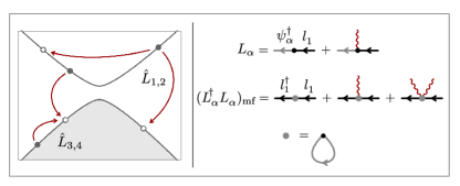
Figure 1: Left: Visualizing the action of the jump operators $\hat{L}$. The operators $\hat{L}_{1,2}$ annihilate particles in the upper band to either re-create them in the lower, or redistribute them in the upper band. Similarly, $\hat{L}_{3,4}$ create particles in the lower band by transfer from the upper or redistribution from the lower band. The stationary state of this process is a fully occupied lower band. Right: A mean field decoupling $\langle{\psi}_{\alpha}^{\,}{\psi}_{\alpha}^{\dagger}\rangle\to n$ reduces the quartic field polynomials $L^{\dagger}L\to l^{\dagger}l$ to quadratic ones. The presence of the wavy line indicates that the $L$-fields carry a non-trivial gauge representation, upgrading them to current operators in the presence of an external vector potential, cf. Eq. (6).

An inspection of the quartic terms shows that their leading contribution to the functional integral, formally equivalent to a one-loop self-consistent Born approximation, comes from replacements such as $l_{1}^{\dagger}\psi_{\alpha}\psi^{\dagger}_{\alpha}l_{1}\to l_{1}^{\dagger}\langle\psi_{\alpha}\psi^{\dagger}_{\alpha}\rangle l_{1}=nl_{1}^{\dagger}l_{1}$ (see Supplemental Material A Note (20) for technical details). Prior to the introduction of gauge fields, the same decoupling applies to all terms of quartic order. In effect, it amounts to a substitution $L^{\,}_{1,2}\to l^{\,}_{1}$, $L^{\,}_{3,4}\to l^{\dagger}_{2}$, and an absorption $\gamma\to n\gamma\equiv\bar{\gamma}$ of the density factor in an effective coupling constant.

At this point, the theory has become quadratic in the fields. Representing the $l$-fields via Eq. (3) through $\psi$’s and doing the Gaussian integrals describing the theory after mean field decoupling, we obtain the retarded and Keldysh Green’s functions ($\gamma_{\mathbf{q}}=\bar{\gamma}d_{\mathbf{q}}$)

$$G^{K}_{\omega,\mathbf{q}}\,=\,-2i\bar{\gamma}\frac{{\mathbf{d}_{\mathbf{q}}\cdot\bm{\sigma}}}{\omega^{2}+\gamma_{\mathbf{q}}^{2}},\quad G^{R}_{\omega,\mathbf{q}}\,=\,\frac{\mathbb{1}}{\omega+i\gamma_{\mathbf{q}}}\,.$$ (5)

Here, the different matrix structure of $G^{R}$ and $G^{K}$ implies the absence of a thermodynamic fluctuation–dissipation relation Kamenev (2011); Sieberer et al. (2016). Moreover, the information on the topological band structure abides in $G^{K}$ (via the matrix $\mathbf{d}_{\mathbf{q}}\cdot\bm{\sigma}$), while $G^{R}$ knows only about the spectral structure through the function $\gamma_{\mathbf{q}}$. The structure of the Green’s function also shows that in mean field theory the many body dissipative damping mechanism reduces to a spectral gap for single-particle excitations, $i\gamma_{\mathbf{q}}\stackrel{{\scriptstyle\mathbf{q}\rightarrow 0}}{{\longrightarrow}}i\bar{\gamma}m^{2}$. Therefore, both, single–particle and particle-hole excitations are gapped out.

Gauge theory – In its present form, the theory describes the relaxation of generic states $\hat{\rho}$ into the Chern insulator dark state $\hat{\rho}_{D}$. We now take the next step to couple the fermions to a gauge field and in this way probe the response to external perturbation. To this end, we go back to the original Keldysh action (4) and notice that it possesses a $\mathrm{U}(1)\times\mathrm{U}(1)$ symmetry under independent phase rotations $\psi_{\sigma}\to e^{i\chi_{\sigma}}\psi_{\sigma}$, $\sigma=\pm$ of the fields on the two contours. On general grounds, phase rotations with spatio-temporal variation generate a finite action cost where $\sum_{\sigma}\int_{t,\mathbf{x}}\sigma\partial_{\mu}\chi_{\sigma}J^{\mu}_{\sigma}$, ($\partial_{\mu}=(\partial_{t},\vec{\nabla})$), and $J^{\mu}_{\sigma}$, define conserved currents of the theory Sieberer et al. (2016). The symmetry under phase rotations is upgraded to a local one by gauging it Avron et al. (2011). We do so by minimally coupling occurrences of phase gradients in Eq. (4) as $\partial_{\mu}\chi_{\sigma}\to\partial_{\mu}\chi_{\sigma}+A_{\sigma,\mu}$ to the components of a vector potential, independently for both contours. In this way, $Z\to Z[A]$ becomes a sourced functional, from which expectation values of currents can be computed as derivatives. Of particular interest are the elements of the DC conductance tensor Mahan (1993), $\sigma_{ij}=\lim_{\omega,\mathbf{q}\to 0}\omega^{-1}\delta^{2}_{A_{q,i,\mathbf{q},\omega},A_{c,j,-\mathbf{q},-\omega}}Z[A]$ , where the Keldysh representation $A_{c}=(A_{+}+A_{-})/2,A_{q}=A_{+}-A_{-}$ is used.

To give these expressions concrete meaning, the coupling of the gauge field to the action needs to be made explicit. From Eq. (4), we infer that the temporal component couples to the action as $\int_{t,\mathbf{x}}\psi^{\dagger}_{\sigma}A_{\sigma,0}\psi_{\sigma}$. The coupling to the spatial components is more interesting, and this is where the interplay of topology and dissipation comes in: consider the jump operator $L_{1}=\psi^{\dagger}_{1}l_{1}$. With $l=V\psi$, phase transformations affect this expression as $L_{1,\sigma}\to L_{1,\sigma}+\psi_{1}^{\dagger}(\partial_{q_{i}}VV^{-1}l)_{1}\,\partial_{i}\chi$, where $\partial_{q_{i}}VV^{-1}$ is a matrix local in momentum space, but non-local in real space. Using that $V_{\mathbf{q}}$ and the unitary diagonalizing matrices $U_{\mathbf{q}}=d_{\mathbf{q}}^{\frac{1}{2}}V_{\mathbf{q}}$ differ only by a scalar factor, we find that, up to an inessential diagonal matrix, $\partial_{q^{i}}VV^{-1}=-ia_{i}+\dots$, where $a_{i}\equiv i\partial_{q_{i}}UU^{-1}$ is the Berry connection defining the topology of the system Asbóth et al. (2016). In this way we conclude that

$$L_{1}\to L_{1}-i\psi_{1}^{\dagger}(a_{i}l)_{1}A_{i}$$ (6)

describes the minimal coupling of the jump operators to both the external gauge field $A_{i}$, and the ‘internal’ gauge field $a_{i}$ (cf. wavy line in the top row of Fig. 1 left.) With this substitution the bilinears $L_{1}^{\dagger}L_{1}^{\,}$ pick up $A$-dependence of up to second order.

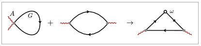
Figure 2: Structure of the diagrams appearing in the expansion in $A$. Both diagrams are individually ultraviolet-divergent in momentum space. The divergences cancel and the remaining contribution is identical to the triangle structure on the right, where the empty dot represents the expansion of the propagators $G$ to first order in the external frequency, $\omega$. This gives a contribution $\sim\omega A_{i}A_{j}$ which becomes one part of the Chern-Simons action.

We next expand the action to second order in $A_{i}$ and apply the same mean field decoupling as that outlined above. This procedure is equivalent to a one-loop approximation of the action (cf. Fig. 2, and Supplemental Material B Note (20) for details). It is reminiscent of the computation of an induced CS term Redlich and Wijewardhana (1985); Dunne in $(2+1)$-dimensional quantum electrodynamics by loop expansion, later proven to be unchanged under the inclusion of higher order gauge invariant gauge–matter interactions Coleman and Hill (1985). Under the condition of purity of the dark state, which is met by the model (2)-(3) , this procedure yields $S[A]=\frac{\theta}{4\pi}\int_{t,\mathbf{x}}\epsilon_{ij}A_{i}\partial_{t}A_{j}$, where the prefactor is given by the Chern number of the filled band, $\theta=-\frac{\pi}{2}\int_{\mathbf{q}}\text{Tr}[\sigma^{z}(\partial_{q_{1}}a_{2}-\partial_{q_{2}}a_{1})]$. The above linear response relation shows that this parameter defines the quantized transverse conductance as $\sigma_{12}=\theta/2\pi$. For the particular two-band model defined above, the identification of $a$ through the transformation matrices (3) leads to the winding number representation $\theta=\frac{1}{4\pi}\int d^{2}q\,\frac{1}{d^{3}}\,\mathbf{d}\cdot(\partial_{q_{1}}\mathbf{d}\times\partial_{q_{2}}\mathbf{d})$, which evaluates to the Chern number $\theta=-1$.

Topological gauge theory – One may now complete the derivation of the topological action by double expansion in the temporal and spatial components $\sim A_{0}A_{i}$. However, there is no need to do so explicitly, because the structure of the ensuing dissipative Chern-Simons action is entirely fixed by symmetry and topological principles. To see how, we note that the most general form of a Chern-Simons action of two gauge fields $(A_{c},A_{q})$ reads $S_{\text{CS}}[A]=\int_{t,\mathbf{x}}{M^{IJ}}A_{I}dA_{J}$, where we switched to a compact differential form notation $\epsilon^{\mu\nu\rho}\,A_{\mu}\partial_{\nu}A_{\rho}\rightarrow AdA$, and $M$ is a $2\times 2$ matrix. Probability conservation (equivalent to the absence of purely $c$ contributions to the action of bosonic Keldysh theory Kamenev (2011)) requires ${M^{cc}}=0$. Similarly, the preserved Hermiticity of a density matrix under evolution by the Keldysh functional requires $S^{*}[A_{c},A_{q}]=-S[A_{c},-A_{q}]$, from which ${M^{cq}=(M^{cq})^{*}\equiv\tilde{M}}$ and ${M^{qq}=-(M^{qq})^{*}}$. The condition that topological actions enter a theory as purely imaginary phases Altland and Simons (2010) in combination with the reality of the vector potential $A$ enforces $M_{qq}=0$. We thus conclude that the most general form of the action consistent with symmetries reads as $S_{\text{CS}}[A]=\tilde{M}\int_{t,\mathbf{x}}(A_{c}dA_{q}+A_{q}dA_{c})$. The quantization of $\tilde{M}$ likewise follows from trace preservation, i.e., probability conservation, but in somewhat different ways : the latter requires that at times $t=\pm\infty$ the Keldysh time contour be closed, which means that time is effectively defined on a circle. Now consider the effect of a gauge transformation, $\psi\to e^{i\chi}\psi$, where $\chi$ is spatially constant and changes uniformly in time to accumulate an integer winding number $2\pi W$ upon completion of the full time revolution. In Keldysh theory the condition that such large gauge transformations be inconsequential enforces the quantization of observables Altland and Egger (2009), and in the present context that of the CS coupling constant. Folding time onto the standard forward and backward contour, the gauge transformation $A\to A+d\chi$ leaves $A_{c}$ invariant, while $A_{q,0}\to A_{q,0}+\frac{2\pi W}{\Delta T}$, where $\Delta T$ is the diverging extent of the Keldysh time interval. Substitution into the action shows that the latter changes by $\frac{2M}{\Delta T}\int_{\Delta T}dt\Phi$, where $\Phi\equiv\int_{\textbf{x}}(\partial_{i}A_{j}-\partial_{j}A_{i})$ is the out of plane magnetic flux through the system. Requiring (Dirac monopole) quantization of the latter, $\Phi=2\pi n$, on a boundary–less spatial domain Tong , we find that the gauge transformation changes the action by an inconsequential multiple of $2\pi$, provided $M=\theta/4\pi$, with integer $\theta$. In agreement with this general argument, the calculation valid for the present model determines $\theta$ as a Chern number, thus respecting the condition.

Summarizing, the above construction identifies

$$S_{\text{CS}}[A] =\frac{\theta}{4\pi}\int_{t,\mathbf{x}}{\epsilon_{\mu\nu\rho}}\,(A_{c,\mu}\partial_{\nu}A_{q,\rho}+A_{q,\mu}\partial_{\nu}A_{c,\rho}),$$ (7)

$$\theta =-\frac{\pi}{2}\int_{\mathbf{q}}\text{Tr}[\sigma^{z}F],\quad F=\partial_{q_{1}}a_{2}-\partial_{q_{2}}a_{1},$$ (8)

as the final form of the topological field theory describing the describing the long-time/distance response of a purely dissipative system with a pure Chern insulator steady state characterized by the Chern number $\theta$.

Boundary theory – In the presence of a system boundary, the Chern-Simons theory (7) lacks gauge invariance Tong . In principle, one may attempt to identify a supplementary boundary theory compensating for this non-invariance by microscopic construction. However, we here adopt the more economical strategy Wen (1995) to reason that gauge invariance is restored if the boundaries harbor a postulated gapless chiral boson mode. The minimal action of this mode reads Wen (1995) $S_{0}[\phi]\equiv-\frac{\theta}{4\pi}\int_{x,t}(\partial_{t}\phi_{c}\partial_{x}\phi_{q}+(q\leftrightarrow c))$, where $x$ is the boundary coordinate. In the presence of an external vector potential, $A_{I}$, this action picks up an additional contribution Stone (1991) $\delta S[\phi,A]\equiv-\frac{\theta}{4\pi}\int_{x,t}(2\partial_{x}\phi_{c}A_{q,0}+2A_{c,0}A_{q,0}+(q\leftrightarrow c))$. Gauge transformations, $A_{I}\to A_{I}-\partial\chi_{I},\phi_{I}\rightarrow\phi_{I}+\chi_{I}$ then affect the full action $S[\phi,A]=S_{0}[\phi]+\delta S[\phi,A]$, in such a way that the full action $S[\phi,A]+S_{\mathrm{CS}}[A]$ is gauge invariant. In the absence of the external field, the boundary particle density is given by $n(x,t)=\delta_{A_{q,0}(x,t)}\big{|}_{A=0}S[\phi,A]=\frac{\theta}{4\pi}\partial_{x}\phi(x,t)$. The above action is minimal in that variation of $S_{0}$ leads to stationarity of the boundary density $\partial_{t}n(x,t)=0$. To add dynamics to $n$, elements outside pure CS theory need to be invoked. Specifically, the so far neglected Hermitian Hamiltonian $\hat{H}_{0}$ will generate unitary time evolution through the operator equation $i\partial_{t}\hat{n}=-[\hat{H}_{0},\hat{n}]$. For example, if $\hat{H}_{0}$ describes a topological insulator, this leads to chiral boundary evolution, $\partial_{t}\hat{n}=v\hat{n}$, with a non-universal velocity $v$. In the boundary theory, this is accounted for by generalization $S_{0}[\phi]\rightarrow-\frac{\theta}{4\pi}\int_{t,x}((\partial_{t}\phi_{c}-v\partial_{x}\phi_{c})\partial_{x}\phi_{q}+(q\leftrightarrow c))$. However, irrespective of the detailed realization of the dynamics, the CS action generated by the dissipative bulk, requires the presence of a gapless boundary mode.

Conclusions and Outlook – We have considered quantum matter defined via a dissipative driving protocol with a topologically twisted dark state. This setting is an antipode to that in topological insulators, where mathematically identical twists are inscribed into the ground state of a non-interacting Hamiltonian. Our main result is that Chern-Simons theory emerges in either case, underpinning the universality of topological gauge theory. In the driven framework, its stabilization rests on three prerequisites: particle number conservation (formally equivalent to a double $\mathrm{U}(1)\times\mathrm{U}(1)$ symmetry separately for the forward and backward time evolution), purity of the dark state, and presence of a dissipative gap. Crucially, however, quantum mechanical unitarity is nowhere required to stabilize the topological response theory.

Finally, one may look at the situation from the perspective of general geometric response theory for Lindbladian dynamics whose formal framework has been developed in the seminal work Avron et al. (2011, 2012a, 2012b); Albert et al. (2016). The present study demonstrates how such structures materialize in concrete settings where nonlinear fermion dynamics stabilizes a system, and a minimal coupling scheme probes it. Given that response theories define an ‘interface’ between the micro– and the macrophysics of a system, this construction may provide useful guiding principles to the description of topologically ordered quantum matter beyond the Hamiltonian ground state setting. Specifically, one may consider the extension to other classes of non-Hermitian systems currently under active research Weimann et al. (2017); Zhou et al. (2018); Gong et al. (2018); Kunst et al. (2018); Kawabata et al. (2019), and strongly entangled out of equilibrium systems with fractional excitations Ma et al. (2019).

Acknowledgements – We thank M. Fleischhauer, M. Goldstein, H. Hansson, S. Moroz and M. Rudner for insightful discussions. We acknowledge support from the Deutsche Forschungsgemeinschaft (DFG, German Research Foundation) under Germany’s Excellence Strategy Cluster of Excellence Matter and Light for Quantum Computing (ML4Q) EXC 2004/1 390534769, and by the DFG Collaborative Research Center (CRC) 183 Project No. 277101999 - project B02. S.D. and F.T. acknowledge support by the European Research Council (ERC) under the Horizon 2020 research and innovation program, Grant Agreement No. 647434 (DOQS). J.C.B. acknowledges financial support from the DFG through SFB 1143 (project-id 247310070) and the Wuerzburg-Dresden Cluster of Excellence ct.qmat (EXC 2147, project-id 39085490).

I Supplemental material

I.1 A.  Self-Consistent Born Approximation

The mean field approximation applied to the dissipative model is analogous to the one-loop self-consistent Born approximation developed for Hamiltonian systems Altland and Simons (2010): each quartic vertex is replaced by sums of bilinears constructed by selecting one couple of fields from the vertex and contracting the other two. For example, for the $++$ vertices involving $l_{1}$, it consists in the replacement

$$l^{\dagger}_{1,+}\psi^{\,}_{\alpha,+}\psi_{\alpha,+}^{\dagger}l_{1,+}^{\,}\to -\langle l^{\dagger}_{1,+}\psi^{\,}_{\alpha,+}\rangle\psi^{\dagger}_{\alpha,+}l^{\,}_{1,+}$$ (9)

$$+\langle\psi^{\dagger}_{\alpha,+}\psi^{\,}_{\alpha,+}\rangle l^{\dagger}_{1,+}l^{\,}_{1,+}+\,_{\cdots}\,,$$

where Einstein’s summation convention is assumed as in the main text, unless otherwise specified. A diagrammatic representation of this procedure is depicted in Fig. 1 in the main text.

Since the vertex is local, all contractions involve fields with the same time (and space) arguments, and the corresponding Green’s functions are singular and need to be regularized by means of a point splitting of the fields. This can be done e.g. as in Sieberer et al. (2016), by introducing an infinitesimal correction to perfect Markovianity.

On the $\pm$ basis, the regularization is needed only for vertices $++$ and $--$, because Green’s functions with crossed indices, $\langle\psi^{\,}_{\pm,\alpha}\psi^{\dagger}_{\mp,\beta}\rangle=iG^{</>}_{\alpha\beta}$ Kamenev (2011), are well-defined also for equal time arguments. For any model described by a Lindbladian, the point-splitting reads $L^{\dagger}_{\pm}(t)L^{\,}_{\pm}(t)\to L^{\dagger}_{\pm}(t\pm\varepsilon)L^{\,}_{\pm}(t)$; the same scheme is applied within each Lindblad operator, e.g., $L_{\pm}=\psi^{\dagger}_{\pm}l^{\,}_{\pm}\to\psi^{\dagger}_{\pm}(t\pm\varepsilon)l^{\,}_{\pm}(t)$. We denote the split by the superscript ${\,}^{(\varepsilon)}$ for brevity. Time/anti-time ordered Green’s functions are now well-defined; for example, in Eq. (9),

$$\langle\psi_{+,\alpha}^{(\varepsilon)}\psi^{\dagger}_{+,\alpha}\rangle=iG^{\mathbb{T}}_{\alpha\alpha}(t=+\varepsilon)=\langle\hat{\psi}_{\alpha}^{\,}\hat{\psi}^{\dagger}_{\alpha}\rangle.$$ (10)

This is a static expectation value of operators, the order of which is fixed. Similar equalities hold for Green’s functions involving all other field and branch index combinations. In particular, it can be shown that all Green’s functions of the same fields but different branch indices correspond to the same operatorial expression, thus reducing the number of independent mean field parameters.

Contractions in Eq. (9) can now be determined. One is already computed in Eq. (10) and is fixed by the half filling condition (see main text), $\langle\psi_{+,\alpha}^{(\varepsilon)}\,\psi^{\dagger}_{+,\alpha}\rangle=n$. The others must be found self-consistently, and read:

$$\langle l^{\dagger\,(\varepsilon)}_{+,1}\,l^{\,}_{+,1}\rangle= \,\langle\hat{l}^{\dagger}_{1}\hat{l}^{\,}_{1}\rangle,$$ (11)

$$\langle\psi^{\dagger\,(\varepsilon)}_{+,\alpha}l^{\,}_{+,1}\rangle= \,\langle\hat{\psi}^{\dagger}_{\alpha}\hat{l}^{\,}_{1}\rangle,\quad\langle l^{\dagger\,(\varepsilon)}_{+,1}\,\psi^{\,}_{+,\alpha}\rangle=\langle\hat{l}^{\dagger}_{1}\hat{\psi}^{\,}_{\alpha}\rangle.$$

The right hand side of Eqs. (11) vanishes if computed on the dark state. This is a feature shared by the analogous contractions coming from all other vertices. Setting them to zero, thus leaving $\langle\psi^{\,}_{\alpha}\psi^{\dagger}_{\alpha}\rangle=n$ as the only nonvanishing contraction, corresponds to the replacement $L\to l,\ \gamma\to\gamma n=\bar{\gamma}$ in the original action, and the resulting model does indeed share the same dark state as the strongly interacting one, fulfilling the self-consistent condition. A more detailed analysis Tonielli et al. (tion) shows that this is the only possible solution, completing the derivation.

I.2 B.  Chern-Simons level

We substantiate here the content of Fig. 2 in the main text, and we also derive Eq. (7), starting from the minimal coupling of the strongly interacting model outlined in the main text. In particular, these results show that the mean field approximation preserves gauge invariance, at least up to first order of the derivative expansion of the gauge action. We proceed on two lines: on one hand, we compute the ultraviolet divergent contributions coming from all the vertices, to prove that the sum vanishes; on the other, we compute only the finite terms necessary to show Eq. (7). We focus for simplicity on the case of a purely spatial gauge field configuration, $A_{\sigma,\mu}=(0,A_{\sigma,i})$; although more involved, the case $A_{\sigma,0}\neq 0$ can be treated in complete analogy.

We recall from the main text that the model couples to the spatial components of the gauge field through shifts of Lindblad operators, expressed by Eq. (6) for $L_{1}$ and by analogous equations for $L_{2,3,4}$. The minimally coupled action has the form $S[\psi,A]=\sum_{i=0}^{2}X^{(i)}$, each $X^{(i)}$ being of $i$th order in $A$ and (up to) quartic in fermionic operators. The gauge action can be obtained by integrating over fermionic degrees of freedom, with action $S[\psi]=X^{(0)}$. Denoting by $S^{(i)}[A]$ the sector of the gauge action of $i$th order in $A$, we get in cumulant expansion in second order in $A$:

$$S^{(1)}[A] =\langle X^{(1)}\rangle,$$ (12a)

$$S^{(2)}[A] =\langle X^{(2)}\rangle+\frac{i}{2}\langle X^{(1)}X^{(1)}\rangle_{c.},$$ (12b)

the subscript $c.$ in Eq. (12b) denoting the connected part of the correlation function, $\langle X^{(1)}X^{(1)}\rangle_{c.}=\langle X^{(1)}X^{(1)}\rangle-\langle X^{(1)}\rangle^{2}$. We work out the full, local contribution of $\langle X^{(1)}\rangle$ and $\langle X^{(2)}\rangle$ to $S[A]$, whereas an expansion in derivatives of the fields is enough to extract the local and Chern-Simons terms from $\langle X^{(1)}X^{(1)}\rangle_{c.}$. More concretely, parametrizing the latter in the Keldysh representation as

$$i\langle X^{(1)}X^{(1)}\rangle_{c.}\equiv\int_{\omega,\mathbf{q}}A^{\,}_{I,i}\Pi^{IJ}_{ij}A^{\,}_{J,j}, I,J\in\{c,q\},$$ (13)

we determine only $\Pi^{IJ}_{ij}(0,\mathbf{0})$ and $\partial_{\omega}\Pi^{cq}_{ij}(0,\mathbf{0})$.

Recalling from the main text the definition of the Berry connection, $a_{i}=i\partial_{q_{i}}UU^{-1}$, and suppressing the Keldysh structure for simplicity, $X^{(i)}$ are integrals of the linear combinations of the following terms:

$$X^{(0)}=\ L^{\dagger}L^{\,},\psi^{\dagger}i\partial_{t}\psi,$$ (14a)

$$X^{(1)}=\ l^{\dagger}_{1}\,\psi^{\,}_{\alpha}\psi^{\dagger\,}_{\alpha}\,(a^{\,}_{i\,}l)^{\,}_{1}\,A^{\,}_{i}\,,\,A^{\,}_{i}\,(a^{\,}_{i\,}l)^{\dagger}_{1}\,\psi^{\,}_{\alpha}\psi^{\dagger\,}_{\alpha}\,l^{\,}_{1}\,,$$ (14b)

$$l^{\,}_{2}\,\psi^{\dagger\,}_{\alpha}\psi^{\,}_{\alpha}\,(a^{\,}_{i\,}l)_{2}^{\dagger}\,A^{\,}_{i}\,,\,A^{\,}_{i}\,(a^{\,}_{i\,}l)^{\,}_{2}\,\psi^{\dagger\,}_{\alpha}\psi^{\,}_{\alpha}\,l^{\dagger}_{2}\,,$$

$$X^{(2)}=\ A^{\,}_{i}\,(a^{\,}_{i\,}l)^{\dagger}_{1}\,\psi^{\,}_{\alpha}\psi^{\dagger\,}_{\alpha}\,(a^{\,}_{j}l)^{\,}_{1}\,A^{\,}_{j}\,,$$ (14c)

$$A^{\,}_{i}\,(a^{\,}_{i\,}l)_{2}^{\,}\,\psi^{\dagger\,}_{\alpha}\psi^{\,}_{\alpha}\,(a^{\,}_{j}l)_{2}^{\dagger}\,A^{\,}_{j}\,,$$

where the order of fields reflects the operatorial ordering of the corresponding terms in the Liouvillian via the point-splitting explained in Sec. A. In Eqs. (14b) and (14c), the gauge fields $A$ have the same contour index $\sigma$ as the operator they are closest in Eqs. (14) to; for example, $A_{i}^{\,}l^{\dagger}{\,}_{\cdots}\equiv A^{\,}_{\sigma,i}l^{\dagger}_{\sigma}{\,}_{\cdots}$, where $\sigma$ is a free and fixed branch index in this case. Moreover, each curly bracket is expanded in band and momentum space as $(a_{i}l)_{\alpha,\mathbf{q}}=a_{i,\alpha\beta,\mathbf{q}\,}l_{\beta,\mathbf{q}}$, with $\alpha,\beta\in\{1,2\}$ band indices.

Without any approximation, we can already infer from Eq. (14b) that $S^{(1)}[A]$ vanishes due to the dark state property, in agreement with the requirement of gauge invariance. In fact, all terms in $X^{(1)}$ either have $l_{1}^{\,}$ or $l^{\dagger}_{2}$ on the right, or their Hermitian conjugates on the left. In both cases, they act directly on the dark state, annihilating it.

To compute the more interesting quadratic sector $S^{(2)}[A]$, that includes the topological action, we adopt the same decoupling scheme employed to obtain the Green’s functions (5). We make in Eqs. (14b) and (14c) the replacements $\psi^{\,}_{\alpha}\psi^{\dagger\,}_{\alpha}\to\langle\psi^{\,}_{\alpha}\psi^{\dagger\,}_{\alpha}\rangle=n$ and $\psi^{\dagger\,}_{\alpha}\psi^{\,}_{\alpha}\to\langle\psi^{\dagger\,}_{\alpha}\psi^{\,}_{\alpha}\rangle=n$.

The main building blocks of the calculations are the static and dynamic correlation functions of the eigenoperators. The former are easier to determine by adopting the point splitting procedure on the basis of contour fields, see Sec. A. They read:

$$\begin{split}\langle l^{\,}_{\sigma,\alpha,\mathbf{p}}l^{\dagger}_{\sigma^{\prime},\alpha^{\prime},\mathbf{p^{\prime}}}\rangle=d_{\mathbf{p}}\delta_{\alpha,1}\delta_{\alpha^{\prime},1}\delta_{\mathbf{p},\mathbf{p}^{\prime}},\\ \langle l^{\dagger}_{\sigma,\alpha,\mathbf{p}}l^{\,}_{\sigma^{\prime},\alpha^{\prime},\mathbf{p^{\prime}}}\rangle=d_{\mathbf{p}}\delta_{\alpha,2}\delta_{\alpha^{\prime},2}\delta_{\mathbf{p},\mathbf{p}^{\prime}}.\end{split}$$ (15)

When the correlation functions are computed at two different times, we find the Keldysh representation more practical. We denote the former by $\tilde{G}\sim-i\langle l\,l^{\dagger}\rangle$ to stress the different field combination as compared to Eq. (5). Keldysh and retarded Green’s functions can be either defined as in the main text, replacing $\psi\to l$, or more compactly after the rotation Kamenev (2011) $l^{1/2}=(l^{+}\pm l^{-})/\sqrt{2}$ and $l^{1/2\dagger}=(l^{+\dagger}\mp l^{+\dagger})/\sqrt{2}$. In this case they can be computed as $i\tilde{G}^{K}_{\alpha\beta}(t)=\langle\psi^{1}_{\alpha}\psi^{2\dagger}_{\beta}\rangle$ and $i\tilde{G}^{R}_{\alpha\beta}(t)=\langle\psi^{1}_{\alpha}\psi^{2\dagger}_{\beta}\rangle$. From Eq. (3) for $l_{1/2}$ and Eq. (5) for $G^{K/R}$, in the frequency and momentum domains we have

$$\tilde{G}^{K}_{\omega,\mathbf{q}}=V^{\,}_{\mathbf{q}}G^{K}_{\omega,\mathbf{q}}V^{\dagger}_{\mathbf{q}}=\frac{-2i\bar{\gamma}d_{\mathbf{q}}^{2}\sigma^{z}}{\omega^{2}+\gamma_{\mathbf{q}}^{2}}\equiv g^{K}_{\omega,\mathbf{q}}\sigma^{z},$$ (16)

$$\tilde{G}^{R}_{\omega,\mathbf{q}}=V^{\,}_{\mathbf{q}}G^{R}_{\omega,\mathbf{q}}V^{\dagger}_{\mathbf{q}}=\frac{d_{\mathbf{q}}\mathbb{1}}{\omega+i\gamma_{\mathbf{q}}}\equiv g^{R}_{\omega,\mathbf{q}}\mathbb{1}.$$

We can now proceed to determine $S^{(2)}[A]$. We denote the decoupled quadratic and linear terms in the gauge field respectively by $X^{(2)}_{m.f.}$ and $X^{(1)}_{m.f.}$. The first contribution corresponds to the first diagram in Fig. 2. Expressing it in terms of $A_{c}$ and $A_{q}$, we get:

$$\langle X^{(2)}_{m.f.}\rangle =i\bar{\gamma}\lambda_{ij}\int_{t,\mathbf{x}}\!A^{\,}_{q,i}A^{\,}_{q,j}-A^{\,}_{c,i}A^{\,}_{q,j}+A^{\,}_{q,i}A^{\,}_{c,j},$$ (17)

$$\lambda_{ij} \equiv\int_{\mathbf{p}}\big{\langle}(a^{\,}_{i\,}l)^{\dagger}_{1,\mathbf{p}}(a^{\,}_{j}l)^{\,}_{1,\mathbf{p}}+(a^{\,}_{i\,}l)_{2,\mathbf{p}}^{\,}(a^{\,}_{j}l)_{2,\mathbf{p}}^{\dagger}\big{\rangle}\,$$ (18)

$$=\int_{\mathbf{p}}\frac{d_{\mathbf{p}}}{2}\,\text{Tr}\big{[}\big{(}a_{i}a_{j}\big{)}_{\mathbf{p}}-\sigma^{z}a_{i,\mathbf{p}}\sigma^{z}a_{j,\mathbf{p}}$$

$$\quad\quad\quad\quad\quad\ -\sigma^{z}\big{(}a_{i}a_{j}-a_{j}a_{i}\big{)}_{\mathbf{p}\,}\big{]},$$

where Tr denotes the trace over band indices. The static expectation values in Eq. (18) involve contour fields, since they are generated independently by each term of the quantum master equation. However, the respective indices are not specified because the expectation values are independent of them, as shown by Eqs. (15).

We move on to the calculation of the connected correlation function $\langle X^{(1)}_{m.f.}X^{(1)}_{m.f.}\rangle^{\,}_{c.}$, which we illustrate by discussing the components of $\Pi^{IJ}_{ij}(\omega,\mathbf{q})$, defined by Eq. (13). The first step is to simplify $X^{(1)}_{m.f.}$ by excluding terms contributing only at order $\mathcal{O}(\mathbf{q})$ of the Taylor expansion of $\Pi^{IJ}_{ij}(\omega,\mathbf{q})$. This can be done by assuming that all eigenoperators in Eq. (14b) have the same momentum argument, leading e.g. to the replacement

$$l^{\dagger}_{\mathbf{p}_{1}}(a^{\,}_{i}l)^{\,}_{\mathbf{p}_{2}}+(a^{\,}_{i\,}l_{\,})^{\dagger}_{\mathbf{p}_{1}}l^{\,}_{\mathbf{p}_{2}}\ \to\ 2l^{\dagger}_{\mathbf{p}_{1}}a^{\,}_{i,(\mathbf{p}_{1}+\mathbf{p}_{2})/2\,}l^{\,}_{\mathbf{p}_{2}}\,.$$ (19)

In all the diagrams we compute, momentum conservation actually implies $\mathbf{p}_{1}=\mathbf{p}_{2}=(\mathbf{p}_{1}+\mathbf{p}_{2})/2$, making the distinction between different field arguments fictitious. The resulting gauge-matter coupling reads:

$$X^{(1)}_{m.f.}=\int 2\bar{\gamma}\,A^{\,}_{c,i}\,l^{1\dagger}_{\,}\big{[}\sigma^{z},a^{\,}_{i}\big{]}l^{2}_{\,}\,-\,\bar{\gamma}\,A^{\,}_{q,i}\,\big{(}l^{2\dagger}_{\,}a_{i}^{\,}l^{1}_{\,}$$ (20)

$$+l^{2\dagger}_{\,}a^{\,}_{i}\sigma^{z}l^{2}_{\,}-\,l^{1\dagger}_{\,}\sigma^{z}a^{\,}_{i}l^{1}_{\,}-\,l^{1\dagger}_{\,}a_{i}^{\,}l^{2}_{\,}\big{)}.$$

The corresponding interaction vertices between matter and spatial components of the gauge field are depicted in Fig. 3.

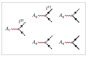
Figure 3: Diagrammatic representation of the interaction between gauge fields and effective currents. Continuous lines stand for $l^{1}/l^{2\dagger}$, dashed lines for $l^{2}/l^{1\dagger}$, and wiggly lines for $A_{c/q}$, with Keldysh index clear from the context in this case.

The simplest term we consider is $\Pi^{cc}_{ij}(0,\mathbf{0})$. It involves only $l^{2}$ and $l^{1\dagger}$, and thus vanishes due to $\langle l^{2}_{\alpha}l_{\beta}^{1\dagger}\rangle=0$.

$\Pi^{qq}_{ij}(0,\mathbf{0})$ is the sum of seven diagrams, depicted in Fig. 4. The first five contribute as:

$$\Pi^{qq}_{ij}(0,\mathbf{0})\big{|}_{(I)}=\, i\bar{\gamma}^{2}\int_{\epsilon,\mathbf{p}}g^{K}\big{(}g^{K}-2g^{R}+2g^{A}\big{)}$$ (21)

$$\quad\quad\cdot\text{Tr}\big{[}\sigma^{z}a_{i,\mathbf{p}}\sigma^{z}a_{j,\mathbf{p}}\big{]}$$

$$=\, i\int_{\epsilon,\mathbf{p}}\frac{4\gamma_{\mathbf{p}}^{4}}{(\omega^{2}+\gamma^{2}_{\mathbf{p}})^{2}}\cdot\text{Tr}\big{[}\sigma^{z}a_{i,\mathbf{p}}\sigma^{z}a_{j,\mathbf{p}}\big{]}$$

$$=\, i\bar{\gamma}\int_{\mathbf{p}}d_{\mathbf{p}}\,\text{Tr}\big{[}\sigma^{z}a_{i,\mathbf{p}}\sigma^{z}a_{j,\mathbf{p}}\big{]},$$

where we omitted the arguments of the Green’s functions for brevity, and used $\gamma_{\mathbf{p}}=\bar{\gamma}d_{\mathbf{p}}$. The last two diagrams in Fig. 4 contribute instead as:

$$\Pi^{qq}_{ij}(0,\mathbf{0})\big{|}_{(II)}=\, -i\bar{\gamma}^{2}\int_{\epsilon,\mathbf{p}}g^{R}g^{A}\,\text{Tr}\big{[}(a_{i}a_{j})_{\mathbf{p}}\big{]}$$ (22)

$$=\, -i\bar{\gamma}\int_{\mathbf{p}}d_{\mathbf{p}}\,\text{Tr}\big{[}(a_{i}a_{j})_{\mathbf{p}}\big{]}.$$

Using Eq. (18) to identify the parameters $\lambda_{ij}$, the sum of the two parts reads:

$$\Pi^{qq}_{ij}(0,\mathbf{0})\big{|}_{(I)+(II)}=-i\bar{\gamma}(\lambda_{ij}+\lambda_{ji}),$$ (23)

that cancels the coefficient of the first term in brackets in Eq. (17), after symmetrizing the latter.

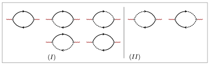
Figure 4: Diagrams contributing to $\Pi^{\,}_{qq}(0,\mathbf{0})$. The two classes of diagrams differ in the matrix structure, see Eqs. (21) and (22).

The last yet most interesting coefficient is $\Pi^{cq}_{ij}$, as it contains the information on the topological invariant: as shown in Fig. 5, the triangle diagram of Fig. 2 plus a diverging local contribution both stem from the diagram contributing to $\Pi^{cq}_{ij}(\omega,\mathbf{0})$ through an expansion in powers of $\omega$. Taking advantage of the simple matrix structure of the Green’s functions of the eigenoperators, we get for the full $\Pi^{cq}_{ij}(\omega,\mathbf{0})$:

$$\Pi^{cq}_{ij}(\omega,\mathbf{0})= -2i\bar{\gamma}^{2}\int_{\epsilon,\mathbf{p}}g^{A}(\epsilon+\omega,\mathbf{p})g^{R}(\epsilon,\mathbf{p})\,$$ (24)

$$\hskip 38.41139pt\cdot\,\text{Tr}\big{[}\sigma^{z}(a_{i}a_{j}-a_{j}a_{i})_{\mathbf{p}}\big{]}=$$

$$= \int_{\mathbf{p}}\frac{\bar{\gamma}^{2}d_{\mathbf{p}}^{2}}{i\gamma_{\mathbf{p}}-\omega/2}\,\text{Tr}\big{[}\sigma^{z}(a_{i}a_{j}-a_{j}a_{i})_{\mathbf{p}}\big{]}.$$

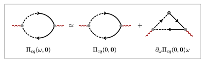
Figure 5: Unique diagram contributing to $\Pi^{\,}_{cq}(\omega,\mathbf{0})$. The Keldysh structure of the triangle diagram can be identified at the first order of the Taylor expansion in $\omega$.

Setting $\omega=0$ and expressing Eq. (24) in terms of $\lambda_{ij}$, it becomes:

$$\Pi^{cq}_{ij}(0,\mathbf{0})=i\bar{\gamma}\big{(}\lambda_{ij}-\lambda_{ji}\big{)}.$$ (25)

This coefficient cancels the analogous one multiplying the second term in brackets in Eq. (17), upon antisymmetrization of the latter. Moreover, both $\Pi^{qc}_{ij}$ and the coefficient of the third term in Eq. (17) are Hermitian conjugates of their $cq$ counterparts, hence they also cancel. The zeroth order of the derivative expansion of $S^{(2)}[A]$ vanishes then exactly, and gauge invariance is preserved as anticipated at the beginning of the section.

At $\mathcal{O}(\omega)$ we get the topological invariant:

$$\omega\,\partial_{\omega}\Pi^{cq}_{ij}(0,\mathbf{0})=\, -\omega\int_{\mathbf{p}}\text{Tr}\big{[}\sigma^{z}(a_{i}a_{j}-a_{j}a_{i})_{\mathbf{p}}\big{]}$$ (26)

$$=\, \frac{i\omega}{2}\,\epsilon_{ij}\,\int_{\mathbf{p}}\text{Tr}\big{[}\sigma^{z}F\big{]}=-i\omega\frac{\mathcal{\theta}}{2\pi}\epsilon_{ij},$$

$F=\partial_{q_{1}}a_{2}-\partial_{q_{2}}a_{1}$ being the Berry curvature, $\theta$ the Chern number of the filled band. Manipulations leading to Eq. (26) are shown below. One part of the Chern-Simons action is recovered after substituting Eq. (26) in $S^{(2)}[A]$, namely $\frac{\theta}{4\pi}\int\epsilon_{ij}A^{\,}_{c,i}\partial_{t}A^{\,}_{q,j}$, (partially) proving the relation (7) between the CS level and the Chern number. The identification $S^{(2)}[A]=S_{\text{CS}}[A]$ at the first order of the derivative expansion of the gauge action can indeed be confirmed by a more complete yet involved calculation Tonielli et al. (tion). We remark that such result extends the proof of gauge invariance up to first order of the derivative expansion of the gauge action, whereas the previous calculation shows it only at the zeroth order.

Let us conclude the section by showing the manipulations leading to the last equality of Eq. (26). First, the definition $a_{i}=i\partial_{q_{i}}UU^{-1}=-iU\partial_{q_{i}}U^{-1}$ implies that

$$a_{1}a_{2}-a_{2}a_{1} =\partial_{q_{1}}U\partial_{q_{2}}U^{-1}-\partial_{q_{2}}U\partial_{q_{1}}U^{-1}$$ (27)

$$=-i(\partial_{q_{1}}a_{2}-\partial_{q_{2}}a_{1})=iF.$$

The last equality follows from the zero sum rule obeyed by the Berry curvatures of the bands, i.e., $\int\text{Tr}\,F=0$ Asbóth et al. (2016).

I.3 C.  Decay of particle-hole excitations

Here we show that the elementary two-body excitation, the creation of a particle in the upper band and a hole in the lower one, is massive in the strongly interacting model.

In the first step, we define the states of interest in terms of normalized eigenoperators as

$$|\mathbf{k}\rangle=n^{-1/2}\int_{\mathbf{q}}\hat{c}^{\dagger}_{1,\mathbf{q}-\mathbf{k}}\hat{c}^{\,}_{2,\mathbf{q}}\,|D\rangle.$$ (28)

They are normalized:

$$\langle\mathbf{k}|\mathbf{k}^{\prime}\rangle =\,n^{-1}\langle D|\int_{\mathbf{q},\mathbf{q}^{\prime}}\hat{c}^{\dagger}_{2,\mathbf{q}\,}\hat{c}^{\,}_{1,\mathbf{q}-\mathbf{k}\,}\hat{c}^{\dagger}_{1,\mathbf{q}^{\prime}-\mathbf{k}^{\prime}\,}\hat{c}^{\,}_{2,\mathbf{q}^{\prime}}\,|D\rangle$$

$$=\,n^{-1}\cdot\delta_{\mathbf{k},\mathbf{k}^{\prime}\,}n=\delta_{\mathbf{k},\mathbf{k}^{\prime}}.$$ (29)

As a second step, we define an effective model that captures the essence of the task, by including only the exactly local processes in the generator of dynamics. This way, we take into account the quick decay of the amplitude of the particle-hole excitations but not its slow, subleading dispersion. The new Lindblad operator describes only direct transitions from the upper band to the lower band, local in real space:

$$\hat{L}(\mathbf{x})=\hat{c}^{\dagger}_{2}(\mathbf{x})\hat{c}^{\,}_{1}(\mathbf{x}) \Leftrightarrow \hat{L}_{\mathbf{k}}=\int_{\mathbf{q}}\hat{c}^{\dagger}_{2,\mathbf{q}-\mathbf{k}}\hat{c}^{\,}_{1,\mathbf{q}}.$$ (30)

The damping strength is set to $\gamma m^{2}$, leading to a mean field dissipative gap equal to $\bar{\gamma}m^{2}$ through the same mean field decoupling explained in the main text, equivalent to $\gamma\to\gamma n=\bar{\gamma}$.

The action of the operator (30) on the state (28) is

$$\hat{L}_{\mathbf{p}}|\mathbf{k}\rangle =\,n^{-1/2}\int_{\mathbf{q},\mathbf{q}^{\prime}}\hat{c}^{\dagger}_{2,\mathbf{q}-\mathbf{p}}\hat{c}^{\,}_{1,\mathbf{q}}\,\hat{c}^{\dagger}_{1,\mathbf{q}^{\prime}-\mathbf{k}}\hat{c}^{\,}_{2,\mathbf{q}^{\prime}}\,|D\rangle$$

$$=\,n^{1/2}\delta_{\mathbf{p},-\mathbf{k}}|D\rangle.$$ (31)

The anticommutator term in the Liouvillian then yields

$$\int_{\mathbf{p}}\hat{L}^{\dagger}_{\mathbf{p}}\hat{L}_{\mathbf{p}}|\mathbf{k}\rangle=n|\mathbf{k}\rangle.$$ (32)

The quantum jump term yields instead

$$\int_{\mathbf{p}}\hat{L}_{\mathbf{p}}|\mathbf{k}\rangle\langle\mathbf{k}|\hat{L}^{\dagger}_{\mathbf{p}}=n|D\rangle\langle D|.$$ (33)

If the initial state is $\hat{\rho}(0)=|\mathbf{k}\rangle\langle\mathbf{k}|$, it follows from Eqs. (32) and (33) that an ansatz for the density matrix at all times can be chosen as

$$\hat{\rho}=\rho_{0}|D\rangle\langle D|+\rho_{\mathbf{k}}|\mathbf{k}\rangle\langle\mathbf{k}|\,.$$ (34)

The closed set of equations for $\rho_{0}$ ($0$ particles, $0$ holes) and $\rho_{\mathbf{k}}$ ($1$ particle, $1$ hole) are:

$$\partial_{t}{\rho}_{0}=2\bar{\gamma}m^{2}\rho_{\mathbf{k}}, \partial_{t}{\rho}_{\mathbf{k}}=-2\bar{\gamma}m^{2}\rho_{\mathbf{k}}.$$ (35)

Eqs. (34) show that the steady state is approached exponentially fast, i.e., that the elementary two-body excitation is gapped.

References

• Thouless et al. (1982) D. J. Thouless, M. Kohmoto, M. P. Nightingale,  and M. den Nijs, Phys. Rev. Lett. 49, 405 (1982).
• Thouless (1983) D. J. Thouless, Phys. Rev. B 27, 6083 (1983).
• Kane and Mele (2005) C. L. Kane and E. J. Mele, Phys. Rev. Lett. 95, 146802 (2005).
• Hasan and Kane (2010) M. Z. Hasan and C. L. Kane, Rev. Mod. Phys. 82, 3045 (2010).
• Qi and Zhang (2011) X.-L. Qi and S.-C. Zhang, Rev. Mod. Phys. 83, 1057 (2011).
• Asbóth et al. (2016) J. K. Asbóth, L. Oroszlány,  and A. Pályi, A Short Course on Topological Insulators, Lecture Notes in Physics, Vol. 919 (Springer International Publishing, Cham, 2016).
• Lindner et al. (2011) N. H. Lindner, G. Refael,  and V. Galitski, Nat. Phys. 7, 490 (2011).
• Rudner et al. (2013) M. S. Rudner, N. H. Lindner, E. Berg,  and M. Levin, Phys. Rev. X 3, 031005 (2013).
• (9) M. S. Rudner and N. H. Lindner,  arXiv:1909.02008 (2019) .
• Diehl et al. (2011) S. Diehl, E. Rico, M. A. Baranov,  and P. Zoller, Nat. Phys. 7, 971 (2011).
• Bardyn et al. (2013) C.-E. Bardyn, M. A. Baranov, C. V. Kraus, E. Rico, A. İmamoğlu, P. Zoller,  and S. Diehl, New J. Phys. 15, 085001 (2013).
• Budich et al. (2015) J. C. Budich, P. Zoller,  and S. Diehl, Phys. Rev. A 91, 042117 (2015).
• Weimann et al. (2017) S. Weimann, M. Kremer, Y. Plotnik, Y. Lumer, S. Nolte, K. G. Makris, M. Segev, M. C. Rechtsman,  and A. Szameit, Nat. Materials 16, 433 (2017).
• Zhou et al. (2018) H. Zhou, C. Peng, Y. Yoon, C. W. Hsu, K. A. Nelson, L. Fu, J. D. Joannopoulos, M. Soljačić,  and B. Zhen, Science (New York, N.Y.) 359, 1009 (2018).
• Gong et al. (2018) Z. Gong, Y. Ashida, K. Kawabata, K. Takasan, S. Higashikawa,  and M. Ueda, Phys. Rev. X 8, 031079 (2018).
• Kunst et al. (2018) F. K. Kunst, E. Edvardsson, J. C. Budich,  and E. J. Bergholtz, Phys. Rev. Lett. 121, 026808 (2018).
• Kawabata et al. (2019) K. Kawabata, K. Shiozaki, M. Ueda,  and M. Sato, Phys. Rev. X 9, 041015 (2019).
• Goldman et al. (2016) N. Goldman, J. C. Budich,  and P. Zoller, Nat. Phys. 12, 639 (2016).
• Lu et al. (2014) L. Lu, J. D. Joannopoulos,  and M. Soljačić, Nat. Photon. 8, 821 (2014).
• Ozawa et al. (2019) T. Ozawa, H. M. Price, A. Amo, N. Goldman, M. Hafezi, L. Lu, M. C. Rechtsman, D. Schuster, J. Simon, O. Zilberberg,  and I. Carusotto, Rev. Mod. Phys. 91, 015006 (2019).
• St-Jean et al. (2017) P. St-Jean, V. Goblot, E. Galopin, A. Lemaître, T. Ozawa, L. Le Gratiet, I. Sagnes, J. Bloch,  and A. Amo, Nat. Photon. 11, 651 (2017).
• Klembt et al. (2018) S. Klembt, T. H. Harder, O. A. Egorov, K. Winkler, R. Ge, M. A. Bandres, M. Emmerling, L. Worschech, T. C. H. Liew, M. Segev, C. Schneider,  and S. Höfling, Nature 562, 552 (2018).
• Zhang et al. (1989) S. C. Zhang, T. H. Hansson,  and S. Kivelson, Phys. Rev. Lett. 62, 82 (1989).
• Lopez and Fradkin (1991) A. Lopez and E. Fradkin, Phys. Rev. B 44, 5246 (1991).
• Kou et al. (2008a) S.-P. Kou, M. Levin,  and X.-G. Wen, Phys. Rev. B 78, 155134 (2008a).
• Qi et al. (2006) X.-L. Qi, Y.-S. Wu,  and S.-C. Zhang, Phys. Rev. B 74, 085308 (2006).
• Redlich (1984) A. N. Redlich, Phys. Rev. D 29, 2366 (1984).
• Ryu et al. (2012) S. Ryu, J. E. Moore,  and A. W. W. Ludwig, Phys. Rev. B 85, 045104 (2012).
• Altland and Bagrets (2016) A. Altland and D. Bagrets, Phys. Rev. B 93, 075113 (2016).
• Wen (1995) X. G. Wen, Adv. Phys. 44, 405 (1995).
• (31) D. Tong,  arXiv:1606.06687 (2016) .
• Kou et al. (2008b) S.-P. Kou, M. Levin,  and X.-G. Wen, Phys. Rev. B 78, 155134 (2008b).
• (33) M. Goldstein,  arXiv:1810.12050 (2018) .
• (34) G. Shavit and M. Goldstein,  arXiv:1903.05336 (2019) .
• Lindblad (1976) G. Lindblad, Comm. Math. Phys. 48, 119 (1976).
• Breuer et al. (2002) H. Breuer, F. Petruccione,  and S. Petruccione, The Theory of Open Quantum Systems (Oxford University Press, 2002).
• Laughlin (1981) R. B. Laughlin, Phys. Rev. B 23, 5632 (1981).
• Note (1) Einstein’s summation convention on repeated indices is assumed unless otherwise specified.
• Kamenev (2011) A. Kamenev, Field theory of non-equilibrium systems (Cambridge University Press, 2011).
• Sieberer et al. (2016) L. M. Sieberer, M. Buchhold,  and S. Diehl, Rep. Prog. Phys 79 (2016).
• Note (20) See Supplemental Material for details on the self-consistent Born approximation, on the evaluation of the prefactor of the Chern-Simons action, and a discussion on the existence of a many-body dissipative gap through a paradigmatic example.
• Note (21) In terms of contour fields, suppressing all arguments but time for simplicity, they are equal to $G^{R}(t)=\theta(t)(G^{>}(t)-G^{<}(t))$ and $G^{K}(t)=G^{>}(t)-G^{<}(t)$, with $iG^{>/<}_{\alpha\beta}(t)=\delimiter 69632778\psi_{\mp,\alpha}^{\tmspace+{.1667em}}(t)\psi_{\pm,\beta}^{\dagger}(0)\delimiter 86414091$ Kamenev (2011).
• Avron et al. (2011) J. E. Avron, M. Fraas, G. M. Graf,  and O. Kenneth, New J. Phys. 13, 053042 (2011).
• Mahan (1993) G. D. Mahan, Many-Particle Physics, 2nd ed. (Plenum, New York, N.Y., 1993).
• Redlich and Wijewardhana (1985) A. N. Redlich and L. C. R. Wijewardhana, Phys. Rev. Lett. 54, 970 (1985).
• (46) G. V. Dunne,  arXiv:902115 (1999) .
• Coleman and Hill (1985) S. Coleman and B. Hill, Phys. Lett. B 159, 184 (1985).
• Note (22) Violations of this condition Tonielli et al. (tion) play a role similar to that of finite temperatures in Hamiltonian settings Dunne and may compromise the form of the Chern-Simons theory.
• Note (23) Despite the lack of thermal symmetry Sieberer et al. (2016), the action (4\@@italiccorr) is invariant under another discrete transformation, namely $\psi_{\pm}^{\tmspace+{.1667em}}\to i\psi^{\dagger}_{\mp}$, $\psi^{\dagger}_{\pm}\to i\psi^{\tmspace+{.1667em}}_{\mp}$, $S\to-S^{*}$, where the latter symbol denotes complex conjugation of the coefficients of the action. This is the field theoretic counterpart of the action of Hermitian conjugation on the Liouvillian. Under this transformation, $S[A_{\pm}]\to-S^{*}[A_{\mp}]$, from which the conditions on $M^{IJ}$ follow.
• Altland and Simons (2010) A. Altland and B. D. Simons, Condensed Matter Field Theory, 2nd ed. (Cambridge University Press, 2010).
• Note (24) While the quantization of coupling constants in non-abelian CS theory is a straightforward consequence of gauge invariance, the situation in abelian theories is somewhat more tricky Tong and depends on the topology of the integration manifold.
• Altland and Egger (2009) A. Altland and R. Egger, Phys. Rev. Lett. 102 (2009).
• Stone (1991) M. Stone, Ann. Phys. 207, 38 (1991).
• Avron et al. (2012a) J. E. Avron, M. Fraas,  and G. M. Graf, J. Stat. Phys. 148, 800 (2012a).
• Avron et al. (2012b) J. Avron, M. Fraas, G. M. Graf,  and P. Grech, Commun. Math. Phys. 314 (2012b).
• Albert et al. (2016) V. V. Albert, B. Bradlyn, M. Fraas,  and L. Jiang, Phys. Rev. X 6, 041031 (2016).
• Ma et al. (2019) R. Ma, B. Saxberg, C. Owens, N. Leung, Y. Lu, J. Simon,  and D. I. Schuster, Nature 566, 51 (2019).
• Tonielli et al. (tion) F. Tonielli, J. C. Budich, A. Altland,  and S. Diehl,   (in preparation).