Angular Correlation Function Estimators Accounting for Contamination from Probabilistic Distance Measurements

Abstract

With the advent of surveys containing millions to billions of galaxies, it is imperative to develop analysis techniques that utilize the available statistical power. In galaxy clustering, even small sample contamination arising from distance uncertainties can lead to large artifacts, which the standard estimator does not account for. We first introduce a formalism, termed decontamination, that corrects for sample contamination by utilizing the observed cross-correlations in the contaminated samples; this corrects any correlation function estimator for contamination. Using this formalism, we present a new estimator that uses the standard estimator to measure correlation functions in the contaminated samples but then corrects for contamination. We also introduce a weighted estimator that assigns each galaxy a weight in each redshift bin based on its probability of being in that bin. We demonstrate that these estimators effectively recover the true correlation functions and their covariance matrices. Our estimators can correct for sample contamination caused by misclassification between object types as well as photometric redshifts; they should be particularly helpful for studies of galaxy evolution and baryonic acoustic oscillations, where forward-modeling the contaminated redshift distribution is undesirable.

1 Introduction

Various probes exist to study the cause of cosmic acceleration, one of which is the evolution of large-scale structure (LSS) as traced by clustering in the spatial distribution of galaxies (Cooray & Sheth, 2002). The standard metric to quantify galaxy clustering is the two-point correlation function (CF) or its Fourier transform, the power spectrum. Galaxy clustering can be measured in 3D using spectroscopic surveys, where precise radial information is available, or by measuring the 2D correlations in tomographic redshift bins when only photometric data is available.

Several large astronomical surveys are coming online in the next decade, allowing access to an unprecedented amount of data and hence the ability to measure the evolution of LSS to high precision. These surveys include the Large Synoptic Survey Telescope (LSST) (LSST Science Collaboration et al., 2009), Dark Energy Spectroscopic Instrument (DESI Collaboration et al., 2016), Euclid (Laureijs et al., 2011), and WFIRST (Spergel et al., 2015). The large datasets, however, present new challenges, among which are understanding, mitigating, and accounting for the impacts of systematic uncertainties that exceed the statistical uncertainties; these include uncertainties due to sample contamination, arising either due to photometric redshift uncertainties or spectroscopic line misidentification. Various studies have presented methods to mitigate these effects; e.g., Elsner et al. (2016) and Leistedt et al. (2016) present mode projection as a way to account for systematics, and Shafer & Huterer (2015) present methodology to handle multiplicative errors like photometric calibration errors.

Various estimators exist to measure the CFs, with the most widely used one introduced in Landy & Szalay (1993) (referred to as LS93 hereafter); see e.g., Kerscher et al. (2000) for a comparison of the various analog estimators, while Vargas-Magaña et al. (2013) and Bernstein (1994) are example studies that consider involved optimizations of the estimators. These estimators can also be extended for various purposes using the overarching idea of ‘marked’ statistics, which employ weights, or ‘marks’, for different quantities: they can be used to account for additional dependencies in the correlation functions (see e.g., Sheth & Tormen, 2004; Harker et al., 2006; Skibba et al., 2006; White & Padmanabhan, 2009; Sheth et al., 2005; Robaina & Bell, 2012; Hernández-Aguayo et al., 2018; White, 2016), extract characteristic-dependent correlations (see e.g., Beisbart & Kerscher, 2000; Armijo et al., 2018), or be used to account for different systematics or to extract target features. For instance, Feldman et al. (1994) present a simple weighting that accounts for the signal-to-noise differences coming from each tomographic volume (which was applied e.g., when measuring the Baryonic Acoustic Oscillations (BAO) in Eisenstein et al. 2005); Ross et al. (2017) extend the weights in Feldman et al. (1994) to handle photometric redshift (photo-$z$) uncertainties for BAO measurements while Peacock et al. (2004) extend them to account for luminosity-dependent clustering, which then are extended by Pearson et al. (2016) for minimal variance in cosmological parameters; Zhu et al. (2015) and Blake et al. (2019) use weights to optimize the BAO measurements; Bianchi et al. (2018) employ weights to account for spectroscopic fibre assignment; Ross et al. (2012) use them to handle systematics, as do Morrison & Hildebrandt (2015); while Bianchi & Percival (2017) and Percival & Bianchi (2017) employ them for 3D correlations to not only correct for missing observations but to improve clustering measurements.

In this paper, we focus on the impacts of sample contamination on the angular correlation functions (ACF). As alluded to earlier, ACFs are especially relevant for photometric surveys, for which we can either measure the projected CFs (e.g., see Zehavi et al. 2002, 2011) or the ACFs in redshift bins (e.g., see Crocce et al. 2016; Balaguera-Antolínez et al. 2018; Abbott et al. 2018). Note that one can also measure the ACFs without the tomographic binning (e.g., as in Connolly et al. 2002; Scranton et al. 2002) but that disallows mapping the evolution of the galaxy clustering. Photo-$z$ uncertainties make measuring ACFs in tomographic bins more challenging as the uncertainties introduce spurious cross-correlations across the redshift bins (e.g., see Bailoni et al. 2017 for a study on the impacts of bin cross-correlations on cosmological parameters) and smear out valuable cosmological information, including the BAO (e.g., as in Chaves-Montero et al. 2018). Since the traditional ACF estimators do not account for contamination arising from photo-$z$ uncertainties, the standard tomographic clustering analysis entails estimating $N(z)$, i.e., the number of galaxies as a function of redshift, in each nominal redshift bin and forward modeling the contaminated ACFs using the $N(z)$ estimates (e.g., as in Crocce et al. 2016; Balaguera-Antolínez et al. 2018; Abbott et al. 2018); also see e.g., Newman (2008) for a discussion on estimating $N(z)$. While this method allows cosmological parameter estimation, it suffers some key limitations as forward modeling is not commonly used outside of cosmology. Furthermore, the variance on the cosmological parameters could potentially be reduced if sample contamination were accounted for directly, instead of being forward modeled, to yield a higher S/N BAO signal from photometric samples.

We propose a method to measure the ACFs while accounting for contamination and without needing to forward model the $N(z)$. Specifically, we first introduce a formalism that uses the observed cross correlations to account for sample contamination. Using this formalism, we propose our first estimator, which still uses the photo-$z$ point estimates and the standard CF estimator, but corrects for contamination. Then, we introduce a new estimator that incorporates not just the photo-$z$ point estimates but each galaxy’s entire photo-$z$ probability distribution function (PDF; of which photo-$z$ is only representative), by weighting each galaxy based on its photo-$z$ PDF. We note that while the second estimator extends the idea of marked statistics, as discussed above, it differs from the applications in the literature on several fronts. In particular, it avoids the loss of information caused by placing galaxies in a single redshift bin based on their photo-$z$s, thereby allowing us to counter the impacts of sample contamination with the statistical power of a large dataset, as well as allowing low-variance measurements of the full correlation function. We return to some of these points for a more thorough discussion of the various differences.

This paper is structured as follows: in Section 2, we formally introduce the ACF and its standard estimator. In Section 3, we introduce terminology to address sample contamination in the most general sense, followed by our first estimator to correct for sample contamination. In Section 4, we introduce a weighted estimator in which the weights can be chosen to track the probability of each galaxy lying in each redshift bin. We present our validation method in Section 5, where we start with a toy example to illustrate the impacts of photo-$z$ uncertainties, followed by a realistic example of measuring the ACFs in three redshift bins, demonstrating the effectiveness of the estimators in recovering the true correlation functions in the presence of sample contamination. We discuss our results in Section 6 and conclude in Section 7.

2 2D Two-Point Correlation Function

The most common statistic to study galaxy clustering is the two-point correlation function. The 2D angular correlation function $w_{\alpha\beta}(\theta)$ measures the excess probability of finding a galaxy of Type-$\alpha$ at an angular distance $\theta$ from a galaxy of Type-$\beta$, in comparison with a random distribution (Peebles, 1993):

$${dP_{\alpha\beta}(\theta)=\eta_{\alpha}\eta_{\beta}\left[{1+w_{\alpha\beta}(\theta)}\right]d\Omega_{\alpha}d\Omega_{\beta}}$$ (1)

where $dP_{\alpha\beta}(\theta)$ is the probability of finding a pair of galaxies of Type-$\alpha\beta$ at an angular distance $\theta$, $\eta_{\alpha}$ is the observed sky density of Type-$\alpha$ galaxies in the projected catalog, and $d\Omega$ is the solid angle element at separation $\theta$. An estimator for the correlation function can be constructed as the ratio of number of data-data pairs compared to the number of random-random pairs at a given angular separation:

$${w_{\alpha\beta}(\theta_{k})=\frac{(DD)_{\alpha\beta}(\theta_{k})}{(RR)_{\alpha\beta}(\theta_{k})}-1}$$ (2)

where $(DD)_{\alpha\beta}(\theta_{k})$ is the normalized number of data-data pairs at angular separation $\theta_{k}$, and $(RR)_{\alpha\beta}(\theta_{k})$ is that for the random-random pairs; the index $k$ emphasizes the binned nature of the estimator. We note that Equation 2 leads to an auto-correlation function when $\alpha=\beta$ and cross-correlation otherwise; for the cross-correlation, we explicitly consider independent random catalogs for the two populations, accounting for the case when the two samples do not completely overlap in their angular range. We also note that each histogram can be written using the Heaviside step function, defined as

$${\Theta(x)=\begin{cases}0,&x<0\\ 1,&x\geq 0\end{cases}}$$ (3)

For instance, for the auto-correlation, we have

$${(DD)_{11}(\theta_{k})=\frac{\sum_{i}^{N_{1}}\sum_{j>i}^{N_{1}}\Theta(\theta_{ij}-\theta_{\mathrm{min},k})[1-\Theta(\theta_{ij}-\theta_{\mathrm{max},k})]}{\sum_{i}^{N_{1}}\sum_{j>i}^{N_{1}}}\equiv\frac{\sum_{i}^{N_{1}}\sum_{j>i}^{N_{1}}\bar{\Theta}_{{ij},k}}{\sum_{i}^{N_{1}}\sum_{j>i}^{N_{1}}}=\frac{\sum_{i}^{N_{1}}\sum_{j\neq i}^{N_{1}}\bar{\Theta}_{{ij},k}}{\sum_{i}^{N_{1}}\sum_{j\neq i}^{N_{1}}}}$$ (4)

where

$${\bar{\Theta}_{{ij},k}\equiv\Theta(\theta_{ij}-\theta_{\mathrm{min},k})[1-\Theta(\theta_{ij}-\theta_{\mathrm{max},k})]}$$ (5)

Here, $\theta_{{ij}}$ is the angular separation between the $i$th and $j$th galaxy in the data sample of ${N_{1}}$ galaxies, and we have explicitly written out the histogram: the $k$th bin counts the number of galaxy pairs at separations $\theta_{\mathrm{min},k}\leq\theta_{ij}<\theta_{\mathrm{max},k}$. Note that the normalized histograms can be calculated either by considering all unique pairs or with double counting, as long as the normalization accounts for the total pairs; the denominator in the case where we count only the unique pairs yields the familiar count of $N_{1}(N_{1}-1)/2$ pairs.

Similar to Equation 4, we can write the histogram for the cross-correlation function as

$${(DD)_{12}(\theta_{k})=\frac{\sum_{i}^{N_{1}}\sum_{j}^{N_{2}}\bar{\Theta}_{{ij},k}}{\sum_{i}^{N_{1}}\sum_{j}^{N_{2}}}}$$ (6)

where sample $\alpha$ contains $N_{\alpha}$ galaxies.

We note here that the estimator in Equation 2 differs only slightly from the estimator introduced in LS93 (referred to hereafter as the LS estimator). In the absence of sample contamination, the LS estimator is unbiased and has Poissonian variance but we choose to work with the simpler estimator since the LS estimator accounts for edge-effects that become subdominant to sample contamination when using large galaxy surveys. Specifically, we note that the $DD/RR$ estimator presented above is as (un)biased as the LS estimator (see Equation 48 in LS93) and its variance reduces to Poissonian variance in the limit of large $N$ (see Equations 42, 48 in LS93).

3 Standard Estimator and Contaminants

We start with the case of two galaxy types in the observed sample, Type-$A$ and Type-$B$; either one acts as a contaminant in relation to the other. We assume that we have some method that gives us the probability of each observed galaxy $i$ of being Type-$A$, $\texttt{q}_{i}^{A}$ or Type-$B$, $\texttt{q}_{i}^{B}$; example methods include, e.g., integration of a galaxy’s photo-$z$ PDF in the target redshift bin or a Bayesian classifier as presented in Leung et al. (2017). Assuming that our observed galaxy sample comprises only the two types of galaxies, we have $\texttt{q}_{i}^{A}+\texttt{q}_{i}^{B}=1$, where $i$ runs over all the galaxies in the observed sample.

Now, assuming that the classifier is unbiased, we can use the classification probabilities to estimate the fraction of objects that are contaminants for a given target sample. For this purpose, however, we must divide the full observed sample into target subsamples, i.e., in the 2-sample case, the observed Type-$A$ and Type-$B$ galaxies. Then, our classifier provides the probability of each observed Type-$A$ galaxy $i$ to be truly of Type-$A$, $q_{i}^{AA}$, as well as the probability of each observed Type-$A$ galaxy to be truly of Type-$B$, $q_{i}^{AB}$. Hence, we have

$${q_{i}^{AA}+q_{i}^{AB}=q_{j}^{BA}+q_{j}^{BB}=1}$$ (7)

where $i$ runs over the observed Type-$A$ sample and $j$ runs over the observed Type-$B$ sample. We can then use the classification probabilities on the observed subsamples to estimate the contamination. That is, we have the fraction of observed Type-$A$ galaxies that are true Type-$A$ or Type-$B$ galaxies given by

$${f_{AA}=\left<{q_{i}^{AA}}\right>\ ;\ f_{AB}=\left<{q_{i}^{AB}}\right>}$$ (8)

where the average is over the observed Type-$A$ sample. Equation 7 translates into the expected identities on the fractions:

$${f_{AA}+f_{AB}=f_{BA}+f_{BB}=1}$$ (9)

These ideas can be generalized to $M$ galaxy samples of Types $A_{1},A_{2},...,A_{M}$, with the classification probabilities on the entire observed sample given by $\texttt{q}_{A_{1}},\texttt{q}_{A_{2}},...,\texttt{q}_{A_{M}}$. Once the full observed catalog is divided into $M$ target subsamples, we have the probability of $i$th observed galaxy of Type-$A_{j}$ being of Type-$A_{m}$ given by $q_{A_{j}A_{m},i}$ and the fraction of observed Type-$A_{j}$ galaxies that are Type-$A_{m}$ galaxies given by $f_{A_{j}A_{m}}$.

3.1 Decontamination

Using the standard ACF estimator, correlations from known contaminated samples can be corrected for by using the fractions $f_{\alpha\beta}$ as defined in Equation 8; see e.g., Grasshorn Gebhardt et al. (2018), Addison et al. (2018) for a similar approach. Formally, this is done by writing the observed correlation functions in terms of the true correlation functions by considering the type of galaxy that contributes to each data pair. Here we work with two target galaxy samples, Type-$A$ and Type-$B$; the generalized case is discussed in Appendix D.1.

Since we have two types of galaxies, we aim to calculate two auto-correlations and one cross-correlation from the contaminated sample: ${w}_{AA}^{{\rm{true}}}(\theta_{k}),{w}_{AB}^{{\rm{true}}}(\theta_{k}),{w}_{BB}^{{\rm{true}}}(\theta_{k})$. However, if we calculate the correlations on the subsamples directly, we get ${w}_{AA}^{{\rm{obs}}}(\theta_{k}),{w}_{AB}^{{\rm{obs}}}(\theta_{k}),{w}_{BB}^{{\rm{obs}}}(\theta_{k})$, which differ from the true correlations due to sample contamination. To construct the relation between the two, lets consider ${w}_{AB}^{{\rm{obs}}}(\theta_{k})$ which gets its contributions from four types of pairs: 1) Observed Type-$A$ galaxies that are true Type-$A$, paired with observed Type-$B$ that are true Type-$A$, contributing $f_{AA}f_{BA}{w}_{AA}^{{\rm{true}}}(\theta_{k})$ to the observed correlation, 2) Observed Type-$A$ that are true Type-$A$, paired with observed Type-$B$ that are true Type-$B$, contributing $f_{AA}f_{BB}{w}_{AB}^{{\rm{true}}}(\theta_{k})$, 3) Observed Type-$B$ that are true Type-$A$, paired with observed Type-$A$ that are true Type-$B$, contributing $f_{AB}f_{BA}{w}_{AB}^{{\rm{true}}}(\theta_{k})$, and 4) Observed Type-$A$ that are true Type-$B$, paired with observed Type-$B$ that are true Type-$B$, contributing $f_{AB}f_{BB}{w}_{BB}^{{\rm{true}}}(\theta_{k})$. Therefore, we have

$${{w}_{AB}^{{\rm{obs}}}(\theta_{k})=f_{AA}f_{BA}{w}_{AA}^{{\rm{true}}}(\theta_{k})+\left\{{f_{AA}f_{BB}+f_{BA}f_{AB}}\right\}{w}_{AB}^{{\rm{true}}}(\theta_{k})+f_{AB}f_{BB}{w}_{BB}^{{\rm{true}}}(\theta_{k})}$$ (10)

The auto correlations follow similarly, leading us to

$${\begin{bmatrix}{w}_{AA}^{{\rm{obs}}}(\theta_{k})\\ {w}_{AB}^{{\rm{obs}}}(\theta_{k})\\ {w}_{BB}^{{\rm{obs}}}(\theta_{k})\end{bmatrix}=\begin{bmatrix}f_{AA}^{2}&2f_{AA}f_{AB}&f_{AB}^{2}\\ f_{AA}f_{BA}&f_{AA}f_{BB}+f_{AB}f_{BA}&f_{AB}f_{BB}\\ f_{BA}^{2}&2f_{BB}f_{BA}&f_{BB}^{2}\end{bmatrix}\begin{bmatrix}{w}_{AA}^{{\rm{true}}}(\theta_{k})\\ {w}_{AB}^{{\rm{true}}}(\theta_{k})\\ {w}_{BB}^{{\rm{true}}}(\theta_{k})\end{bmatrix}}$$ (11)

where we note that the contribution from the true cross correlation to the observed auto correlations simplifies (as opposed for that to the observed cross correlation). We also present a derivation of the result above using Equation 1 in Appendix A.1. Now, using these equations, we can construct the estimators $\widehat{w}_{AA}(\theta_{k}),\widehat{w}_{BB}(\theta_{k}),\widehat{w}_{AB}(\theta_{k})$ for the true correlation functions ${w}_{AA}^{{\rm{true}}}(\theta_{k}),{w}_{BB}^{{\rm{true}}}(\theta_{k}),{w}_{AB}^{{\rm{true}}}(\theta_{k})$ given by

$${\begin{bmatrix}\widehat{w}_{AA}(\theta_{k})\ \ \widehat{w}_{AB}(\theta_{k})\ \ \widehat{w}_{BB}(\theta_{k})\end{bmatrix}^{T}=[D_{\rm{S}}]^{-1}\begin{bmatrix}{w}_{AA}^{{\rm{obs}}}(\theta_{k})\ \ {w}_{AB}^{{\rm{obs}}}(\theta_{k})\ \ {w}_{BB}^{{\rm{obs}}}(\theta_{k})\end{bmatrix}^{T}}$$ (12)

where $[D_{\rm{S}}]$ is the square matrix in Equation 11, which must be invertible. Appendix D.1 presents the Decontaminated estimators for the generalized case of working with $M$ target subsamples.

Given their construction, the Decontaminated estimators are unbiased (under the assumption that the contamination fractions are represented by the average classification probabilities); see Appendix A.2 for more details. As for the variance, the decontamination leads to a quadrature sum of the variance of the standard estimators for each of the auto- and cross-correlations ; the closed form expression for the variance of the estimators is presented in Appendix A.3. Note that this overarching idea of using contamination fractions is similar to that presented in Benjamin et al. (2010) but their focus is on estimating the contamination fractions from the contaminated correlations, for which they resort to approximating the decontamination matrix as diagonal. Since we expect sufficiently strong correlations across the different target samples (e.g., between the neighboring photo-$z$ bins for a tomographic clustering analysis), the simplification of ignoring some contamination fractions becomes undesirable.

4 A New, Weighted Estimator

Here, we present an estimator for the observed correlation function that accounts for pair weights, i.e., each pair of galaxies is weighted to account for its contribution to the target correlation function, e.g., by the classification probability of each contributing galaxy (alongside other parameters). This way, we consider the entire observed catalog, containing $N_{\rm{tot}}$ galaxies of both Type-$A$ and Type-$B$, each with their respective classification probabilities. That is, we propose a Weighted estimator for the observed correlation function:

$${\widetilde{w}_{\alpha\beta}^{\rm{obs}}(\theta_{k})=\frac{(\widetilde{DD})_{\alpha\beta}(\theta_{k})}{RR(\theta_{k})}-1}$$ (13)

where $\alpha,\beta$ are the types, e.g., $\widetilde{w}_{AA}^{\rm{obs}}$ denotes the estimator for the observed Type-$A$ auto-correlation while $\widetilde{w}_{AB}^{\rm{obs}}$ denotes the cross-correlation. Here, we define weighted data-data pair counts as

$${(\widetilde{DD})_{\alpha\beta}(\theta_{k})=\frac{\sum_{i}^{N_{\rm{tot}}}\sum_{j\neq i}^{N_{\rm{tot}}}\texttt{w}_{ij}^{\alpha\beta}\bar{\Theta}_{{ij},k}}{\sum_{i}^{N_{\rm{tot}}}\sum_{j\neq i}^{N_{\rm{tot}}}\texttt{w}_{ij}^{\alpha\beta}}}$$ (14)

where $\texttt{w}_{ij}^{\alpha\beta}$ is the pair weight, with the pair comprised of the $i$th and $j$th galaxies, while the weighting is over all $N_{\rm{tot}}$ galaxies in the observed catalog. We note that the normalization is needed to match the normalization of unweighted correlation functions (Equations 4, 6). Equation 14 therefore allows us to calculate the different weighted data-data pair counts, e.g., $(\widetilde{DD})_{AA},(\widetilde{DD})_{AB},(\widetilde{DD})_{BB}$. We also note that $RR(\theta_{k})$ is formally $(RR)_{\alpha\beta}(\theta_{k})$ since different galaxy samples can have different selection functions. However, since we consider all the galaxies in the observed sample, not just the target subsamples, we take $RR(\theta_{k})$ to trace the full survey geometry. We include some notes on the implementation of the Weighted estimator in Appendix C.2.

In the simplest scenario, the pair weight could be linearly dependent on the probabilities of $i$th and $j$th objects being of Type $\alpha,\beta$ respectively, i.e., $\texttt{w}_{ij}^{\alpha\beta}=\texttt{w}_{i}^{\alpha}\texttt{w}_{j}^{\beta}=\texttt{q}_{i}^{\alpha}\texttt{q}_{j}^{\beta}$. Note that this approach does not require us to break the observed sample into target subsamples as long as intelligent weights are assigned to each galaxy pair. Explicitly, if we have two observed galaxy types in our observed catalog, as was discussed at the beginning of Section 3, $\texttt{w}_{i}^{A}=q_{i}^{AA}$ for observed Type-$A$ while $\texttt{w}_{i}^{A}=q_{i}^{BA}$ for observed Type-$B$ galaxies. Similarly, $\texttt{w}_{i}^{B}=q_{i}^{AB}$ for observed Type-$A$ while $\texttt{w}_{i}^{B}=q_{i}^{BB}$ for observed Type-$B$. Also note that $N_{\rm{tot}}={N}_{{\rm{obs}}}^{A}+{N}_{{\rm{obs}}}^{B}={N}_{{\rm{true}}}^{A}+{N}_{{\rm{true}}}^{B}$. Finally, we highlight that our Weighted estimator reduces to the Standard estimator if $\texttt{w}_{i}^{\alpha}$ is set to 1 for observed Type-$A$ galaxies and to 0 for observed Type-$B$ galaxies, and $\texttt{w}_{i}^{\beta}$ is set to 0 for observed Type-$A$ galaxies and to 1 for observed Type-$B$.

4.1 Estimator Bias and Variance

The estimator in Equation 13 is biased, as it considers the entire sample, including contaminants with different correlation functions. In order to estimate the true correlations using unbiased estimators, $\widehat{w}$, we require that their expectation value approach the true correlations. That is, we have

$${\left<{\begin{bmatrix}\widehat{w}_{AA}(\theta_{k})\\ \widehat{w}_{AB}(\theta_{k})\\ \widehat{w}_{BB}(\theta_{k})\end{bmatrix}}\right>=\left<{[D_{W}]\begin{bmatrix}{\widetilde{w}}_{AA}^{{\rm{obs}}}(\theta_{k})\\ {\widetilde{w}}_{AB}^{{\rm{obs}}}(\theta_{k})\\ {\widetilde{w}}_{BB}^{{\rm{obs}}}(\theta_{k})\end{bmatrix}}\right>=\begin{bmatrix}{w}_{AA}^{{\rm{true}}}(\theta_{k})\\ {w}_{AB}^{{\rm{true}}}(\theta_{k})\\ {w}_{BB}^{{\rm{true}}}(\theta_{k})\end{bmatrix}}$$ (15)

where $[D_{\rm{W}}]$ is a decontamination matrix, designed to make the estimators unbiased. It is analogous to the decontamination matrix $[D_{\rm{S}}]$ in Equation 12. Here we explicitly work with the two-sample case, with only Type-$A$ and Type-$B$ galaxies present in our sample.

As done to decontaminate the Standard estimators in Section 3.1, we calculate the contributions that are coming from each of the true correlation functions to any given weighted correlation function. That is, we have

$$\begin{split}\left<{\widetilde{w}_{\alpha\beta}^{\rm{obs}}(\theta_{k})}\right>&=\frac{\left({\sum\limits_{i}^{N_{\rm{tot}}}\sum\limits_{j\neq i}^{N_{\rm{tot}}}\texttt{w}_{ij}^{\alpha\beta}\texttt{q}_{i}^{A}\texttt{q}_{j}^{A}}\right){w}_{AA}^{{\rm{true}}}(\theta_{k})+\left({\sum\limits_{i}^{N_{\rm{tot}}}\sum\limits_{j\neq i}^{N_{\rm{tot}}}\texttt{w}_{ij}^{\alpha\beta}\left\{{\texttt{q}_{i}^{A}\texttt{q}_{j}^{B}+\texttt{q}_{i}^{B}\texttt{q}_{j}^{A}}\right\}}\right){w}_{AB}^{{\rm{true}}}(\theta_{k})+\left({\sum\limits_{i}^{N_{\rm{tot}}}\sum\limits_{j\neq i}^{N_{\rm{tot}}}\texttt{w}_{ij}^{\alpha\beta}\texttt{q}_{i}^{B}\texttt{q}_{j}^{B}}\right){w}_{BB}^{{\rm{true}}}(\theta_{k})}{\sum\limits_{i}^{N_{\rm{tot}}}\sum\limits_{j\neq i}^{N_{\rm{tot}}}\texttt{w}_{ij}^{\alpha\beta}}\end{split}$$ (16)

We present the full derivation of Equation 16 in Appendix B. Consolidating the terms as done in Equation 11, we have

$${\begin{bmatrix}\left<{{\widetilde{w}}_{AA}^{{\rm{obs}}}(\theta_{k})}\right>\\ \left<{{\widetilde{w}}_{AB}^{{\rm{obs}}}(\theta_{k})}\right>\\ \left<{{\widetilde{w}}_{BB}^{{\rm{obs}}}(\theta_{k})}\right>\end{bmatrix}=\begin{bmatrix}\frac{\sum\limits_{i}^{N_{\rm{tot}}}\sum\limits_{j\neq i}^{N_{\rm{tot}}}\texttt{w}_{ij}^{AA}\texttt{q}_{i}^{A}\texttt{q}_{j}^{A}}{\sum\limits_{i}^{N_{\rm{tot}}}\sum\limits_{j\neq i}^{N_{\rm{tot}}}\texttt{w}_{ij}^{AA}}&\frac{\sum\limits_{i}^{N_{\rm{tot}}}\sum\limits_{j\neq i}^{N_{\rm{tot}}}\texttt{w}_{ij}^{AA}\left\{{\texttt{q}_{i}^{A}\texttt{q}_{j}^{B}+\texttt{q}_{i}^{B}\texttt{q}_{j}^{A}}\right\}}{\sum\limits_{i}^{N_{\rm{tot}}}\sum\limits_{j\neq i}^{N_{\rm{tot}}}\texttt{w}_{ij}^{AA}}&\frac{\sum\limits_{i}^{N_{\rm{tot}}}\sum\limits_{j\neq i}^{N_{\rm{tot}}}\texttt{w}_{ij}^{AA}\texttt{q}_{i}^{B}\texttt{q}_{j}^{B}}{\sum\limits_{i}^{N_{\rm{tot}}}\sum\limits_{j\neq i}^{N_{\rm{tot}}}\texttt{w}_{ij}^{AA}}\\ \frac{\sum\limits_{i}^{N_{\rm{tot}}}\sum\limits_{j\neq i}^{N_{\rm{tot}}}\texttt{w}_{ij}^{AB}\texttt{q}_{i}^{A}\texttt{q}_{j}^{A}}{\sum\limits_{i}^{N_{\rm{tot}}}\sum\limits_{j\neq i}^{N_{\rm{tot}}}\texttt{w}_{ij}^{AB}}&\frac{\sum\limits_{i}^{N_{\rm{tot}}}\sum\limits_{j\neq i}^{N_{\rm{tot}}}\texttt{w}_{ij}^{AB}\left\{{\texttt{q}_{i}^{A}\texttt{q}_{j}^{B}+\texttt{q}_{i}^{B}\texttt{q}_{j}^{A}}\right\}}{\sum\limits_{i}^{N_{\rm{tot}}}\sum\limits_{j\neq i}^{N_{\rm{tot}}}\texttt{w}_{ij}^{AB}}&\frac{\sum\limits_{i}^{N_{\rm{tot}}}\sum\limits_{j\neq i}^{N_{\rm{tot}}}\texttt{w}_{ij}^{AB}\texttt{q}_{i}^{B}\texttt{q}_{j}^{B}}{\sum\limits_{i}^{N_{\rm{tot}}}\sum\limits_{j\neq i}^{N_{\rm{tot}}}\texttt{w}_{ij}^{AB}}\\ \frac{\sum\limits_{i}^{N_{\rm{tot}}}\sum\limits_{j\neq i}^{N_{\rm{tot}}}\texttt{w}_{ij}^{BB}\texttt{q}_{i}^{A}\texttt{q}_{j}^{A}}{\sum\limits_{i}^{N_{\rm{tot}}}\sum\limits_{j\neq i}^{N_{\rm{tot}}}\texttt{w}_{ij}^{BB}}&\frac{\sum\limits_{i}^{N_{\rm{tot}}}\sum\limits_{j\neq i}^{N_{\rm{tot}}}\texttt{w}_{ij}^{BB}\left\{{\texttt{q}_{i}^{A}\texttt{q}_{j}^{B}+\texttt{q}_{i}^{B}\texttt{q}_{j}^{A}}\right\}}{\sum\limits_{i}^{N_{\rm{tot}}}\sum\limits_{j\neq i}^{N_{\rm{tot}}}\texttt{w}_{ij}^{BB}}&\frac{\sum\limits_{i}^{N_{\rm{tot}}}\sum\limits_{j\neq i}^{N_{\rm{tot}}}\texttt{w}_{ij}^{BB}\texttt{q}_{i}^{B}\texttt{q}_{j}^{B}}{\sum\limits_{i}^{N_{\rm{tot}}}\sum\limits_{j\neq i}^{N_{\rm{tot}}}\texttt{w}_{ij}^{BB}}\\ \end{bmatrix}\begin{bmatrix}{w}_{AA}^{{\rm{true}}}(\theta_{k})\\ {w}_{AB}^{{\rm{true}}}(\theta_{k})\\ {w}_{BB}^{{\rm{true}}}(\theta_{k})\end{bmatrix}}$$ (17)

Therefore, the Decontaminated Weighted estimators are given by

$${\begin{bmatrix}\widehat{w}_{AA}(\theta_{k})\ \ \widehat{w}_{AB}(\theta_{k})\ \ \widehat{w}_{BB}(\theta_{k})\end{bmatrix}^{T}=[D_{\rm{W}}]^{-1}\begin{bmatrix}{\widetilde{w}}_{AA}^{{\rm{obs}}}(\theta_{k})\ \ {\widetilde{w}}_{AB}^{{\rm{obs}}}(\theta_{k})\ \ {\widetilde{w}}_{BB}^{{\rm{obs}}}(\theta_{k})\end{bmatrix}^{T}}$$ (18)

where $[D_{\rm{W}}]$ is the square matrix in Equation 17. We note that each row in Equation 18 corresponds to final, unbiased weights on each pair, comprised of a sum of three weights – a fact that can be utilized when optimizing weights for minimum variance. We present an example optimization that decontaminates while estimating the correlation functions in Appendix C.3.

We have checked Equation 18 in various limiting cases to confirm the validity of its form. Specifically, we first divided the total observed sample into subsamples, and then applied the simplifications that reduce the Decontaminated Weighted estimators to Decontaminated estimators (i.e., setting the pair weights for the target subsample to unity and the rest to zero, and approximating the classification probabilities with their averages); we confirm that Equation 18 does indeed reduce to Equation 12. We then tested the two limiting cases of no contamination and 100% contamination, working with just the observed subsamples and using pair weights that are a linear product of the respective classification probabilities; we confirm that the reduced estimator recovers the truth when there is no contamination while it is indeterminate when there is 100% contamination. Finally, we considered the entire observed sample and tested the limiting cases of no contamination and 100% contamination, with pair weights that are a linear product of the respective classification probabilities, and arrive at true correlations both when there is no contamination and when there is 100% contamination – an advantage of using the full sample. We also present the analytical form of the variance of the Weighted estimator in Appendix C.1; since the variance is a function of a four-point sum and depends non-trivially on the pair weights, we choose to estimate the variance numerically. Finally, we present the generalized estimator, i.e., applicable to $M$ target samples, in Appendix D.2.

5 Validation and Results

In order to test our estimators, we consider the simplest relevant application: tomographic clustering analysis, i.e., the measurement of the ACF for galaxies in different redshift bins. Then, in the context of our terminology in Sections 3-4, the different ‘types’ of galaxies are essentially the galaxies in the different redshift bins. For this purpose, we use the publicly available v0.4_r1.4 of MICE-Grand Challenge Galaxy and Halo Light-cone Catalog. The catalog is generated by populating the dark matter halos in MICE, which is an $N$-body simulation covering an octant of the sky at $0\leq z\leq 1.4$. Most importantly for our purposes, the catalog follows local observational constraints, e.g., galaxy clustering as a function of luminosity and color, and incorporates galaxy evolution for realistic high-$z$ clustering – allowing for a robust test of the estimators. More details about the catalog can be found in MICE publications: Fosalba et al. (2015a); Crocce et al. (2015); Fosalba et al. (2015b); Carretero et al. (2015); Hoffmann et al. (2015). We query the catalog using CosmoHub (Carretero et al., 2017).

In order to test our method, we must have photo-$z$s that are realistic for upcoming surveys like LSST. Since MICE catalog photo-$z$s are biased and exhibit a large scatter, we simulate adhoc photo-$z$s using the true redshifts and assuming $\sigma_{z}=0.03(1+z)$, the upper limit on the scatter mentioned in the LSST Science Requirements Document. Specifically, we model the photo-$z$ probability distribution function (PDF) for each galaxy as a Gaussian with its true redshift as the mean and $\sigma_{z}$ as the standard deviation. Then, we randomly draw from the PDF and assign the draw as the photo-$z$ of the galaxy; the “observed PDF” is then a Gaussian with the random draw as the mean and $\sigma_{z}$ as the standard deviation. This method generates unbiased photo-$z$s in a simple way.

Figure 1 illustrates our simulated photo-$z$s: the left panel compares the MICE catalog photo-$z$s and the simulated photo-$z$s with the true redshifts, while the right panel shows $N(z)$, the number of galaxies as a function of redshift, as estimated by binning the redshifts as well as by stacking the photo-$z$ PDFs. We see that our simulated photo-$z$ PDFs and the consequent photo-$z$s effectively recover the overall true galaxy number distribution. Also note that the $N(z)$ from simulated photo-$z$ (solid red) and observed (solid black) PDFs are very similar, indicating that our simulated observed photo-$z$ PDFs are nearly unbiased.

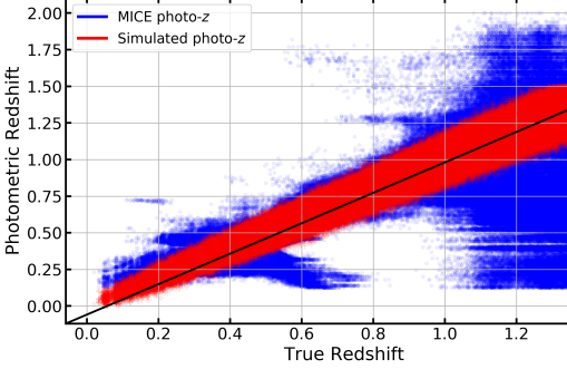
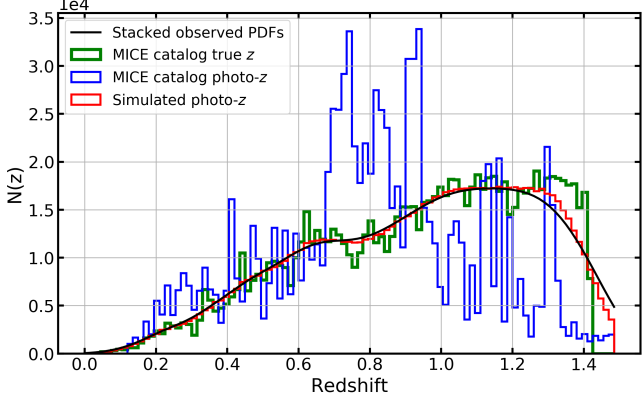
Figure 1: Illustration of the simulated photo-$z$s. Left: Comparison between true redshift and MICE catalog photo-$z$s vs. those simulated here . Right: Comparison between the different $N(z)$ distributions: true $N(z)$; those based on MICE catalog photo-$z$s vs. those simulated assuming Gaussian PDFs with $\sigma_{z}=0.03(1+z)$. The red, blue, green are $N(z)$ estimates from binning the respective redshifts, while the black curve is based on stacking the observed photo-$z$ PDFs. We see that our simulated photo-$z$s are well-behaved and are able to recover the true $N(z)$ effectively. These plots are created using only the galaxies with $0\leq$ RA $\leq 5$ deg, $0\leq$ Dec $\leq 5$ deg, yielding 994,863 galaxies at $0\leq z\leq 1.4$.

Now, the true catalog essentially consists of the location of the galaxies on the sky (RA, Dec) and the true redshift, while the observed catalog consists of the RA, Dec and photo-$z$s. In order to test the effects of contamination, we must work with observed subsamples, i.e., galaxies with photo-$z$s in the target redshift bin; these differ from the true subsamples, which are galaxies with their true redshifts in the target redshift bins. Note that this subsampling is not necessary for the Weighted estimator, introduced in Section 4, which only needs the photo-$z$ PDFs for all the observed galaxies. We use TreeCorr (Jarvis et al., 2004) to calculate the correlation functions.

5.1 Toy Example

In order to illustrate the impacts of photo-$z$s, we consider a toy example: a clustering analysis using only two tomographic bins ($0.7\leq z<0.8$, $0.8\leq z<0.9$) with the true galaxy sample having galaxies only at $0.75\leq z\leq 0.76$, $0.85\leq z\leq 0.86$, but with the photo-$z$ scatter as mentioned before, i.e., $\sigma_{z}=0.03(1+z)$. We query the true galaxies in nine 10x10 deg² patches along Dec = 0; all patches have a similar number of galaxies (66K-78K) and face similar photo-$z$ contamination rates (22-25%, 18-21% in the two tomographic bins, respectively). Figure 2 shows the distributions of the true and photometric redshifts using one of the patches (with 66,927 galaxies, and 23% and 20% contamination in the two tomographic bins, respectively).

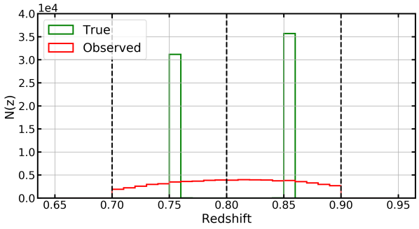
Figure 2: True and observed redshift histograms for the idealized galaxy sample of Section 5.1, with redshift bin edges shown using the vertical dashed lines. We see that photo-$z$ uncertainties lead to a smearing of the redshift information.

Then, using the observed PDFs, we calculate the classification probabilities as the integral of the PDFs within the target redshift bin. Note that since we are simulating only two bins, we use Gaussian PDFs truncated at $z=0.7$ and $z=0.9$ to ensure that we conserve the number of true and observed galaxies; this yields a slight bias in the PDF integrations, which we correct to make the overall classification probabilities unbiased, i.e., $\left<{q_{i}^{AB}}\right>=f_{AB}$, where the average is checked over redshift intervals with $\Delta z=0.02$. Figure 3 shows the distribution of the final classification probabilities for all the galaxies in our observed sample.

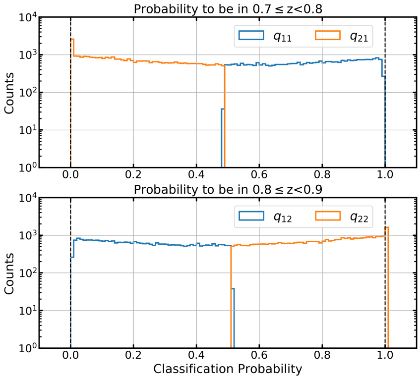
Figure 3: Distribution of the classification probabilities to be in bin 1 (upper panel) or bin 2 (lower panel) for the toy galaxy sample of Section 5.1. As introduced in Section 3, $q_{\alpha\beta}$ is the probability of the observed Type-$\alpha$ galaxy to be a true Type-$\beta$ galaxy. We see that given the photo-$z$ uncertainties, the probability to be in a given target tomographic bin has a broad range.

In order to estimate the various correlation functions (two auto, one cross) and their variance, we consider the 9 patches: the mean across the nine samples gives us the mean estimate of the respective correlation function while we calculate the estimator variance as $\left<{\left\{{\widehat{w}_{i}(\theta_{k})-{w}_{i}^{{\rm{true}}}(\theta_{k})}\right\}^{2}}\right>$ where $i$ runs over all the correlations (both auto and cross) and the expectation value is over all the realizations; note that this variance is not sensitive to the sample variance but only a measure of the estimator variance, which we can calculate explicitly given that we have access to the true CFs in each of the nine patches. Note that for each of the patches, we calculate five types of the three correlation functions: those in the true subsamples; those using the Standard estimator on the contaminated observed subsamples, followed by those from the Decontaminated estimators; and those using the Weighted estimator, followed by the Decontaminated Weighted ones. Also, we use a random catalog that is 5x the size of the data catalog, and restrict to 0.01-3deg scales. Figure 4 shows our results, with both the correlation functions and their variance. As expected, the cross correlations with contamination are non-negligible, taking signal away from the two auto-correlations. find that both estimators correct for the contamination and reduce the bias, leading to estimates closer to the truth. This is more apparent in Figure 5, where we show the bias in the correlation functions (i.e., difference from the truth). We note that the Decontaminated Weighted estimator is unbiased after decontamination – a reassuring result.

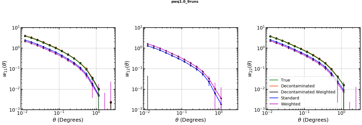
Figure 4: Correlation functions and the variance in the toy galaxy sample with only two redshift bins (presented in Section 5.1). We see that just as Decontamination (red) recovers the truth (green) using the correlations on the contaminated subsamples (blue), the Decontaminated Weighted estimator (black) recovers the truth from the Weighted correlations on the entire observed sample (magenta), without needing to divide the observed sample into subsamples.

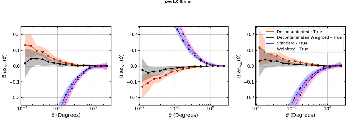
Figure 5: Bias in correlation functions for the toy galaxy sample of Section 5.1, with 1$\sigma$ uncertainties in each estimator indicated with the shaded regions. We see that the Decontaminated Weighted estimator (black) leads to a bias smaller than that from the Decontaminated estimator (red)

5.2 Realistic Example: Optimistic Case

Now we consider a more realistic scenario: a true galaxy sample with $0.7\leq z\leq 1.0$, with three redshift bins ($0.7\leq z<0.8$, $0.8\leq z<0.9$, $0.9\leq z<1.0$) for the tomographic clustering analysis. As before, we query the galaxies in nine 10x10 deg² patches along Dec = 0; all patches have similar number of galaxies (1080K-1147K) and face similar contamination (23-26%, 44-46%, 19-23% in the three tomographic bins, respectively). Note that our chosen bins are realistic, as a tomographic analysis for 10 redshift bins with $\Delta z=0.1$ is currently planned for dark energy science studies with LSST (The LSST Dark Energy Science Collaboration et al., 2018).

Figure 6 shows the distributions of the true redshifts and the photo-$z$s using one of the patches (with 1,095,404 galaxies, and 24%, 45% and 22% contamination in the three redshift bins, respectively). We note that the middle bin sees the largest and most realistic contamination – the case that will be true for most of the LSST bins, hence making this example a relevant one. Note that the bin edges see the impacts of artificially having contamination from only one side.

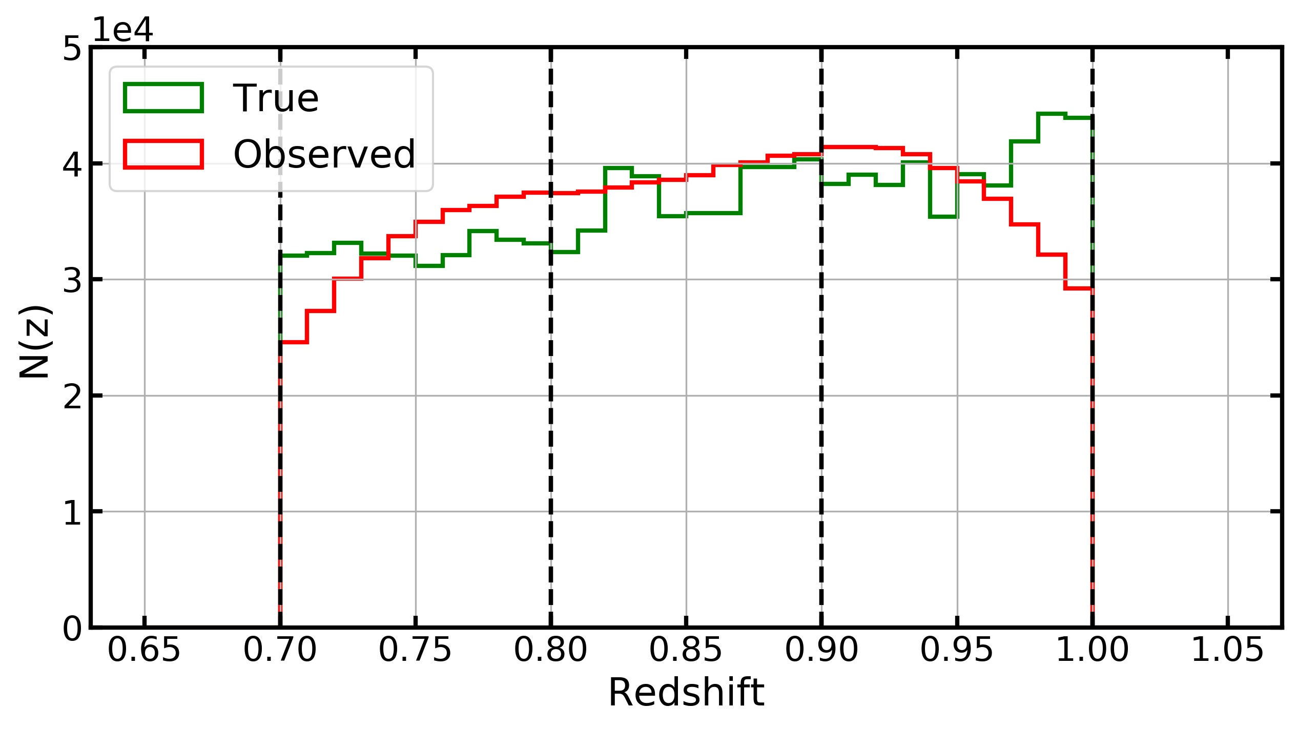
Figure 6: True and observed redshift histograms for the galaxy sample of Section 5.2, with bin edges shown using the vertical dashed lines. We see that the photo-$z$ uncertainties lead to a smearing of the redshift information, while the truncation of the edge-bins makes the $N(z)$ biased near the outermost edges.

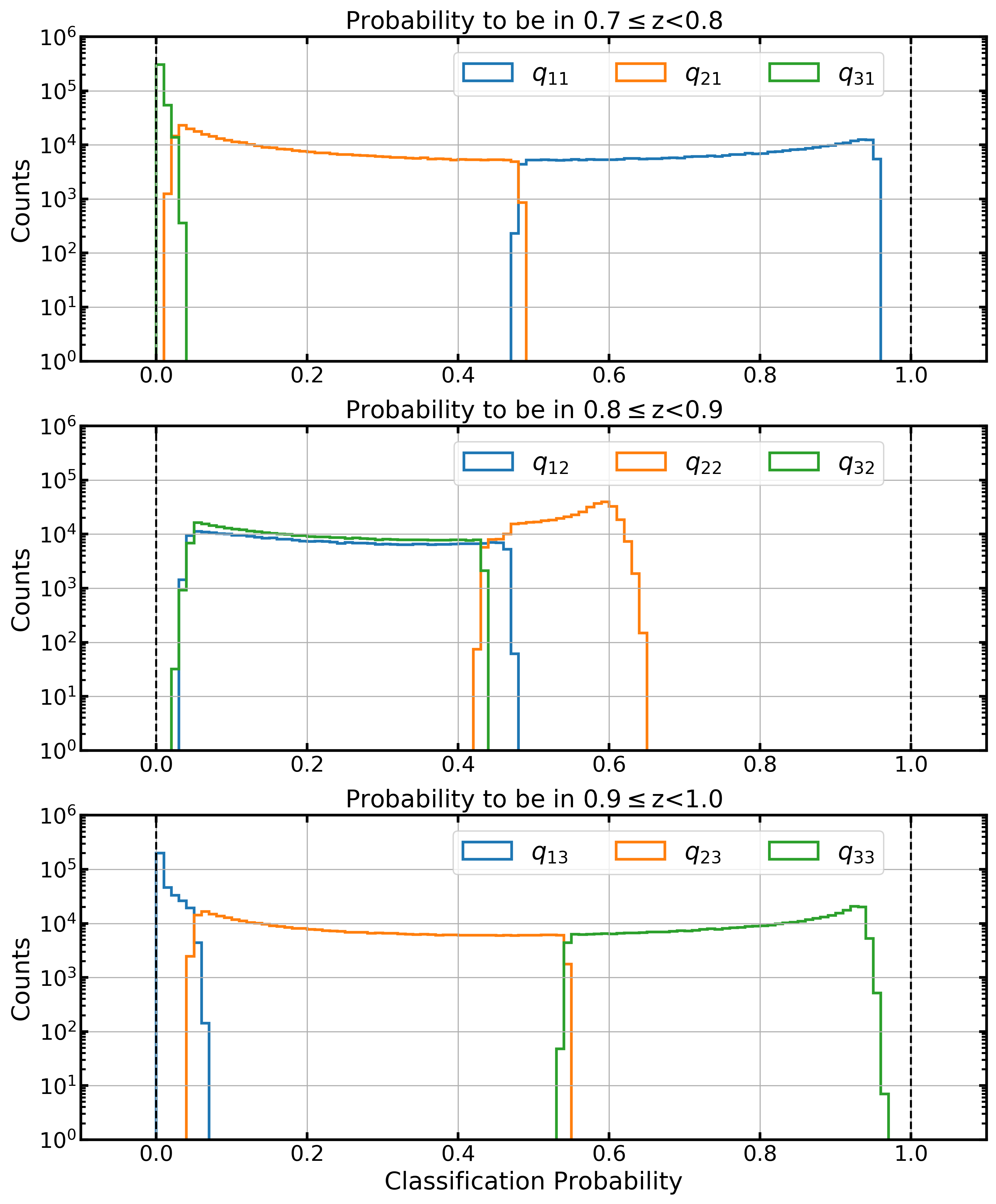
Figure 7: Distribution of the classification probabilities to be in the three target redshift bins for the galaxy sample of Section 5.2. The middle bin sees the largest contamination and therefore has no objects that have a very high probability to be in any target bin.

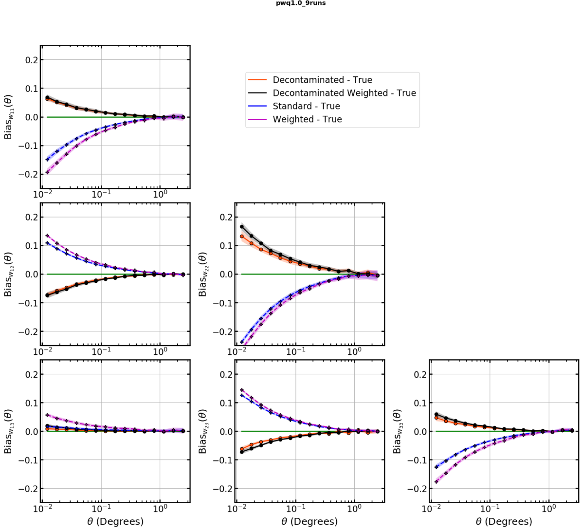
Figure 8: Bias in the correlation functions in the three sample case of Section 5.2, with 1$\sigma$ uncertainties in each estimator indicated with the shaded regions. We see that as in the toy example in Section 5.1, just as Decontamination (red) reduces the bias using the correlations on the contaminated subsamples (blue), the Decontaminated Weighted estimator (black) reduces the bias from the Weighted correlations on the entire observed sample (magenta), without needing to divide the observed sample into subsamples.

Figure 7 shows the distribution of the classification probabilities for all the galaxies. Again we note that given the large contamination rates for the middle bin, the classification probabilities are far from unity, indicating that no observed galaxy has a very high probability to be in any target bin. As before, we calculate the various correlations for each of the nine patches and estimate the mean and the variance across the calculations. Figure 8 illustrates our results, showing only the estimator bias for brevity, where we see that the Decontaminated Weighted estimator leads to a bias that is comparable to that using the Decontaminated estimator. We note that the Decontaminated estimator performs similar to Decontaminated Weighted, potentially due to the correlation functions in the three redshift bins being similar.

As a more comprehensive metric for comparing the various estimators, we consider the covariances in correlation functions across the three redshift bins for an example $\theta$-bin. Specifically, given that we have access to the truth here, we first calculate the covariances in the estimators without accounting for the LSS sample variance – this we term as the “estimator covariance” and calculate as $\left<{\left\{{\widehat{w}_{i}(\theta_{k})-{w}_{i}^{{\rm{true}}}(\theta_{k})}\right\}\left\{{\widehat{w}_{j}(\theta_{k})-{w}_{j}^{{\rm{true}}}(\theta_{k})}\right\}}\right>$ where $i,j$ run over all the correlations (both auto and cross) and the expectation value is over all the realizations; note here that the diagonal of this covariance matrix is the estimator variance used to generate uncertainties shown in Figures 4-5 and Figure 8. We show the estimator covariances for the galaxy sample considered here in Figure LABEL:fig:_3bin_est_cov, where we see that without decontamination, the covariances are large, as expected given the strong mixing of the samples. Both decontaminated estimators effectively reduce the covariances, with Decontaminated Weighted outperforming Decontaminated.

Then we consider the covariances accounting for the LSS sample variance – this we term as the “full covariance” and calculate as $\left<{\left\{{\widehat{w}_{i}(\theta_{k})-\left<{\widehat{w}_{i}(\theta_{k})}\right>}\right\}\left\{{\widehat{w}_{j}(\theta_{k})-\left<{\widehat{w}_{j}(\theta_{k})}\right>}\right\}}\right>$ where $i,j$ again run over all the correlations and the expectation value is over all the realizations; these are shown in Figure LABEL:fig:_3bin_full_cov. We see that without decontamination, the clustering information is smeared across the CF-space and is much in contrast from the true covariances. However, both of our decontaminated estimators are able to approximate the true covariances effectively, hence achieving their purpose of correcting for sample contamination. We also note here that decontamination does not simply diagonalize the covariance matrices but instead reduces off-diagonal elements appropriately; diagonalization would not account for true covariances that exist between auto- and cross- CFs for neighboring bins due to shared LSS. Finally, comparing with Figure LABEL:fig:_3bin_est_cov, we note that LSS sample variance largely dominates over the estimator variance for the 10x10 patches considered here – a reassuring result; a comparison between the two sources of variance for larger effective survey area is left for future work.

This completes the demonstration of our new estimators: they provide for a way to decontaminate correlations, while the Weighted estimator specifically allows using the full photo-$z$ PDFs and full observed samples, in a framework that can be extended e.g., to minimize variance.

6 Discussion

We have presented a formalism to estimate the ACFs in the presence of sample contamination arising from photo-$z$ uncertainties. We achieve this by utilizing the probabilistic information available via each galaxy’s photo-$z$ PDF. As mentioned in Section 1, our method avoids forward modeling the contaminated ACFs based on estimated $N(z)$, which is the standard way to handle the photo-$z$  contamination . We note, however, that forward modeling is effective if the contamination can be modeled effectively; a full investigation of measurements using our method vs. those using forward modeling is left for future work. We also note that the BAO signal is washed out by projection and hence its measurement should benefit from our approach.

Our estimators are distinct from previous work employing weighted correlation functions, specifically on three accounts: 1) our weighted estimator considers all galaxies in the entire observed sample as a part of every photo-$z$ bin, 2) to our knowledge, there is no literature on the usage of a decontamination matrix to correct for correlation function contamination, and our Decontaminated Weighted estimator presents a novel way to decontaminate marked correlation functions, and 3) we weight only the data, and not the randoms. In a further comparison with our work, for instance, Ross et al. (2017) employ weights to account for photo-$z$ uncertainty by weighting both the data and random galaxies in the target subsamples by inverse-variance weights. Blake et al. (2019) also weight both the data and random galaxies to increase the precision with which they can measure the BAO by accounting for the dependency on the environment of the measured signal. In somewhat of a contrast, Zhu et al. (2015) use both weighted data and random pairs, and unweighted random pairs for optimized BAO measurements, while Morrison & Hildebrandt (2015) employ weighted randoms to account for mitigating survey systematics. Percival & Bianchi (2017), on the other hand, upweight only their data (data-data, data-random pairs, but not the random-random pairs) for 3D BAO measurements when the spectroscopic data is available only for a subset of the angular sample.

Since this work introduces a new estimator, we note various avenues for further development. For the 2D case, we can optimize the estimator to be minimum variance by introducing an additional parameter for each pair of galaxies, i.e., $\texttt{w}_{ij,\rm{opt}}^{\alpha\beta}$= $\Upsilon_{ij}(q,k)\texttt{w}_{ij}^{\alpha\beta}$, where $\Upsilon_{ij}(q,k)$ are the optimization parameters that minimize the variance of the estimator for each bin $k$. We note that the Decontaminated estimator presented in the text is in fact a special case of the Decontaminated Weighted estimator, with the weights set to 1 when the probability is high enough to place an object in a given subsample and 0 otherwise. It is surprising that the Decontaminated estimator performs nearly as well as our Decontaminated probability-Weighted estimator; this implies either a broad range of optimal weights or, more likely, that the optimal weights lie somewhere between these two simplistic approaches. Optimization of the weights will be an important aspect of applying the new estimator. Furthermore, since we have introduced general pair weights, we can incorporate Bayesian priors on the correlation functions, based on current measurements, or when measuring correlation functions for different galaxy types, as then, we can incorporate priors that are dependent on the separations, e.g., accounting for one galaxy sample clustering strongly on smaller scales. This will call for an in-depth analysis of the covariance matrices for the various correlation functions. Also, we can extend the weighting scheme to harmonic space, where it will be relevant for a tomographic analysis for LSST (Awan et al., in prep).

We also note that our method can handle other kinds of contamination, e.g., star-galaxy contamination, where probabilistic models for whether an object is a star or a galaxy can inform the weights for each object in our observed sample . Finally, we can also extend the 2D formulation to 3D, where it will be relevant for HETDEX (Hill et al., 2008), Euclid and WFIRST, as they face emission line contaminants, as well as LSST where the projected correlation function will be measurable (without tomographic binning). Note that for the 3D case in real space, we must treat the random catalogs more carefully than in 2D; in the 2D case, we have not made a distinction between random catalogs for the different samples as they are spatially overlapping with the same selection function – a case that does not hold for 3D.

7 Conclusions

Cosmology is entering a data-driven era, with several upcoming galaxy surveys opening gateways for huge galaxy catalogs. Given the increased statistical power of our datasets, we face imminent challenges, including the need to account for systematic uncertainties that dominate the uncertainty budget on our measurements. In this paper, we have studied the treatment of contamination arising from photo-$z$ uncertainties when measuring the two-point angular correlation functions. We first introduced a simple formalism: decontamination that uses the correlations in contaminated subsamples to estimate the true correlations. We then introduced a new estimator that accounts for the full photo-$z$ PDF of each galaxy to estimate the true correlations, allowing each galaxy to contribute to all bins (or samples) based on their probabilities. We demonstrated the effectiveness of our method on both a toy example and a realistic scenario that is scaleable for surveys like LSST.

We emphasize the need for more data-driven tools in order to truly utilize the statistical power of the large datasets. Here we have presented an estimator that incorporates the available probabilistic information to reduce the variance in the measured correlation functions; this represents a step in the direction of reducing biases and uncertainties in the measurement of cosmological parameters from upcoming surveys.

Appendix A Decontaminated Estimator: Decontamination, Bias and Variance

A.1 Decontamination Derivation

Here, we re-derive the decontamination equation (Equation 11) using the definition of angular correlation function. We start with Equation 1, rewriting it as

$$\begin{split}dP_{\alpha\beta}(\theta_{k})&=\eta_{\alpha\beta}^{\rm{pair}}\left[{1+w_{\alpha\beta}(\theta_{k})}\right]d\Omega_{\alpha}d\Omega_{\beta}=\mathcal{N}_{\alpha\beta}\left[{1+w_{\alpha\beta}(\theta_{k})}\right]\frac{d\Omega_{\alpha}}{V_{\alpha}}\frac{d\Omega_{\beta}}{V_{\beta}}\end{split}$$ (A1)

where $\eta_{\alpha\beta}^{\rm{pair}}$ is the observed sky density of Type-$\alpha\beta$ pairs of galaxies while $\mathcal{N}_{\alpha\beta}$ is the observed number of type-$\alpha\beta$ pairs. Assuming that we work with large surveys such that the integral constraint is nearly zero, $\mathcal{N}_{\alpha\beta}\rightarrow\left<{\mathcal{N}_{\alpha\beta}}\right>$, hence the simplification in the last line in the equation above. Since we consider samples in the same volume, $V_{\alpha}=V_{\beta}=V$ and $d\Omega_{\alpha}=d\Omega_{\beta}=d\Omega$. Therefore, for the Standard estimator, where we have the correlations measured in the contamination subsamples, we have

$$\begin{split}dP_{\alpha\beta}(\theta_{k})=\mathcal{N}_{\alpha\beta,\rm{obs}}\left[{1+w_{\alpha\beta}^{\rm{obs}}(\theta_{k})}\right]\frac{d\Omega}{V}\frac{d\Omega}{V}=\sum_{\gamma,\delta}\mathcal{N}_{\alpha\beta,\rm{obs}}^{\gamma\delta,\rm{true}}[1+w_{\gamma,\delta}^{\rm{true}}(\theta_{k})]\frac{d\Omega}{V}\frac{d\Omega}{V}\end{split}$$ (A2)

where $w_{\alpha\beta}^{\rm{obs}}(\theta_{k})$ is the biased correlation function, measured using contaminated samples. Expanding the sum on the right hand side, we have

$$\begin{split}\mathcal{N}_{\alpha\beta,\rm{obs}}^{\rm{tot}}\left[{1+w_{\alpha\beta}^{\rm{obs}}(\theta_{k})}\right]&=\mathcal{N}_{\alpha\beta,\rm{obs}}^{11,\rm{true}}\left[{1+w_{11}^{\rm{true}}(\theta_{k})}\right]+\mathcal{N}_{\alpha\beta,\rm{obs}}^{12,\rm{true}}\left[{1+w_{12}^{\rm{true}}(\theta_{k})}\right]\\ &\hskip 20.00003pt+\mathcal{N}_{\alpha\beta,\rm{obs}}^{21,\rm{true}}\left[{1+w_{21}^{\rm{true}}(\theta_{k})}\right]+\mathcal{N}_{\alpha\beta,\rm{obs}}^{22,\rm{true}}\left[{1+w_{22}^{\rm{true}}(\theta_{k})}\right]\end{split}$$ (A3)

Since we have

$${\frac{\mathcal{N}_{\alpha\beta,\rm{obs}}^{\gamma\delta,\rm{true}}}{\mathcal{N}_{\alpha\beta,\rm{obs}}^{\rm{tot}}}=f_{\alpha\gamma}f_{\beta\delta}}$$ (A4)

$${\Rightarrow\left[{1+w_{\alpha\beta}^{\rm{obs}}(\theta_{k})}\right]=f_{\alpha 1}f_{\beta 1}\left[{1+w_{11}^{\rm{true}}(\theta_{k})}\right]+\left\{{f_{\alpha 1}f_{\beta 2}+f_{\alpha 2}f_{\beta 1}}\right\}\left[{1+w_{12}^{\rm{true}}(\theta_{k})}\right]+f_{\alpha 2}f_{\beta 2}\left[{1+w_{22}^{\rm{true}}(\theta_{k})}\right]}$$ (A5)

Therefore, for $\alpha,\beta=1,2$, Equation A5 becomes

$${\left[{1+w_{12}^{\rm{obs}}(\theta_{k})}\right]=f_{11}f_{21}\left[{1+w_{11}^{\rm{true}}(\theta_{k})}\right]+\left\{{f_{11}f_{22}+f_{12}f_{21}}\right\}\left[{1+w_{12}^{\rm{true}}(\theta_{k})}\right]+f_{12}f_{22}\left[{1+w_{22}^{\rm{true}}(\theta_{k})}\right]}$$ (A6)

Now, since

$$\begin{split}f_{11}f_{21}+\left\{{f_{11}f_{22}+f_{12}f_{21}}\right\}+f_{12}f_{22}=f_{11}\left[{f_{21}+f_{22}}\right]+f_{12}\left[{f_{21}+f_{2}}\right]=1,\end{split}$$ (A7)

we have

$$\begin{split}w_{12}^{\rm{obs}}(\theta_{k})&=f_{11}f_{21}w_{11}^{\rm{true}}(\theta_{k})+\left\{{f_{11}f_{22}+f_{12}f_{21}}\right\}w_{12}^{\rm{true}}(\theta_{k})+f_{12}f_{22}w_{22}^{\rm{true}}(\theta_{k})\end{split}$$ (A8)

which agrees with Equation 11. Similar results follow for $(\alpha,\beta)$ = (1,1), (2, 2).

A.2 Estimator Bias

We expect that the Decontaminated estimators are unbiased given their construction (i.e., Equation 10). However, for brevity, we formally show that they are indeed unbiased. By definition, an unbiased estimator is such that

$${\left<{\widehat{w}}\right>=w_{\rm{true}}}$$ (A9)

where the expectation value is over many realizations of the survey. Then, using Equations 11 and 12, we have

$$\begin{split}\left<{\begin{bmatrix}\widehat{w}_{AA}(\theta_{k})\ \ \widehat{w}_{AB}(\theta_{k})\ \ \widehat{w}_{BB}(\theta_{k})\end{bmatrix}^{T}}\right>&=\left<{[D_{\rm{S}}]^{-1}\begin{bmatrix}{w}_{AA}^{{\rm{obs}}}(\theta_{k})\ \ {w}_{AB}^{{\rm{obs}}}(\theta_{k})\ \ {w}_{BB}^{{\rm{obs}}}(\theta_{k})\end{bmatrix}^{T}}\right>\\ &=[D_{\rm{S}}]^{-1}[D_{\rm{S}}]\begin{bmatrix}{w}_{AA}^{{\rm{true}}}(\theta_{k})\ \ {w}_{AB}^{{\rm{true}}}(\theta_{k})\ \ {w}_{BB}^{{\rm{true}}}(\theta_{k})\end{bmatrix}^{T}=\begin{bmatrix}{w}_{AA}^{{\rm{true}}}(\theta_{k})\ \ {w}_{AB}^{{\rm{true}}}(\theta_{k})\ \ {w}_{BB}^{{\rm{true}}}(\theta_{k})\end{bmatrix}^{T}\end{split}$$ (A10)

where the second equality follows by substituting Equation 11. Hence, the Decontaminated estimators are unbiased. We note here that $[D_{\rm{S}}]$ in Equation 12 is effectively a decontamination matrix: it removes the contamination from the biased estimates, $w_{\alpha\beta}^{\rm{obs}}$, in the presence of sample contamination. A similar argument follows for the case where we have $M$ target samples, using Equation D4. We also note that Equation A10 is valid only when $f_{\alpha\beta}$ are accurate averages of the classification probabilities.

A.3 Estimator Variance

As for the variance of the Decontaminated estimator, we can calculate it by using the variance in our observed correlations. That is, given Equation 12, we have

$${\begin{bmatrix}\sigma_{\widehat{w}_{AA}}^{2}(\theta_{k})\ \ \sigma_{\widehat{w}_{AB}}^{2}(\theta_{k})\ \ \sigma_{\widehat{w}_{BB}}^{2}(\theta_{k})\end{bmatrix}^{T}=\left\{{[D_{\rm{S}}]^{-1}}\right\}_{ij}^{2}\begin{bmatrix}\sigma_{{w}_{AA}^{{\rm{obs}}}}^{2}(\theta_{k})\ \ \sigma_{{w}_{AB}^{{\rm{obs}}}}^{2}(\theta_{k})\ \ \sigma_{{w}_{BB}^{{\rm{obs}}}}^{2}(\theta_{k})\end{bmatrix}^{T}}$$ (A11)

Appendix B Decontamination: From Decontaminated with Full Sample to Weighted

Here, we present the methodology to decontaminate the Weighted correlation function introduced in Equation 13, using the formalism introduced in A.1. To develop intuition, we first extend the methodology in A.1 to consider an unweighted full observed sample, followed by considering the weighted full sample.

B.1 Decontaminated: Full Sample

We extend the treatment in A.1 to consider an unweighted full sample. Then, the analog of Equation A2 is

$$\begin{split}dP(\theta_{k})=\mathcal{N}_{\rm{tot_{obs}}}\left[{1+w^{\rm{full}}(\theta_{k})}\right]\frac{d\Omega}{V}\frac{d\Omega}{V}=\sum_{\gamma,\delta}\mathcal{N}_{\rm{tot_{obs}}}^{\gamma\delta,\rm{true}}[1+w_{\gamma,\delta}^{\rm{true}}(\theta_{k})]\frac{d\Omega}{V}\frac{d\Omega}{V}\end{split}$$ (B1)

Note that we have dropped the $\alpha,\beta$ markers since there is only one correlation that can be measured for the unweighted full sample. Expanding the sum, we have

$$\begin{split}\mathcal{N}_{\rm{tot_{obs}}}\left[{1+w^{\rm{full}}(\theta_{k})}\right]&=\mathcal{N}_{\rm{tot_{obs}}}^{11,\rm{true}}\left[{1+w_{11}^{\rm{true}}(\theta_{k})}\right]+\mathcal{N}_{\rm{tot_{obs}}}^{12,\rm{true}}\left[{1+w_{12}^{\rm{true}}(\theta_{k})}\right]\\ &\hskip 20.00003pt+\mathcal{N}_{\rm{tot_{obs}}}^{21,\rm{true}}\left[{1+w_{21}^{\rm{true}}(\theta_{k})}\right]+\mathcal{N}_{\rm{tot_{obs}}}^{22,\rm{true}}\left[{1+w_{22}^{\rm{true}}(\theta_{k})}\right]\end{split}$$ (B2)

Now if we assume that our classification probabilities are unbiased, we can write

$$\begin{split}\sum_{i}^{N_{\rm{tot_{obs}}}^{\gamma}}\sum_{j\neq i}^{N_{\rm{tot_{obs}}}^{\delta}}\texttt{q}_{i}^{\gamma}\texttt{q}_{j}^{\delta}&=\widehat{\mathcal{N}}_{\rm{tot_{obs}}}^{\gamma\delta,\rm{true}}\end{split}$$ (B3)

Note that technically $N_{\rm{tot_{obs}}}^{\gamma}=N_{\rm{tot_{obs}}}^{\delta}=N_{\rm{tot_{obs}}}$ but we keep $\gamma,\delta$ tags just to keep track of samples when reducing to Decontaminated. Now, simplifying the equation above, we have

$$\begin{split}\mathcal{N}_{\rm{tot_{obs}}}\left[{1+w^{\rm{full}}(\theta_{k})}\right]&=\sum_{i}^{N_{\rm{tot_{obs}}}^{1}}\sum_{j\neq i}^{N_{\rm{tot_{obs}}}^{1}}\texttt{q}_{i}^{1}\texttt{q}_{j}^{1}\left[{1+w_{11}^{\rm{true}}(\theta_{k})}\right]+\sum_{i}^{N_{\rm{tot_{obs}}}^{1}}\sum_{j\neq i}^{N_{\rm{tot_{obs}}}^{2}}\texttt{q}_{i}^{1}\texttt{q}_{j}^{2}\left[{1+w_{12}^{\rm{true}}(\theta_{k})}\right]\\ &\hskip 20.00003pt+\sum_{i}^{N_{\rm{tot_{obs}}}^{2}}\sum_{j\neq i}^{N_{\rm{tot_{obs}}}^{1}}\texttt{q}_{i}^{2}\texttt{q}_{j}^{1}\left[{1+w_{21}^{\rm{true}}(\theta_{k})}\right]+\sum_{i}^{N_{\rm{tot_{obs}}}^{2}}\sum_{j\neq i}^{N_{\rm{tot_{obs}}}^{2}}\texttt{q}_{i}^{2}\texttt{q}_{j}^{2}\left[{1+w_{22}^{\rm{true}}(\theta_{k})}\right]\end{split}$$ (B4)

We now check what happens when we reduce the above equation to Decontaminated, i.e., we consider not the full sample but the target subsamples, while all the probabilities are represented by their averages. Then, for $\alpha,\beta=1,2$, Equation B4 becomes

$$\begin{split}N_{1,\rm{obs}}N_{2,\rm{obs}}\left[{1+w_{11}^{\rm{obs}}(\theta_{k})}\right]&=\left({\sum_{i}^{N_{1,\rm{obs}}}\sum_{j\neq i}^{N_{2,\rm{obs}}}\texttt{q}_{i}^{1}\texttt{q}_{j}^{1}}\right)\left[{1+w_{11}^{\rm{true}}(\theta_{k})}\right]+\left({\sum_{i}^{N_{1,\rm{obs}}}\sum_{j\neq i}^{N_{2,\rm{obs}}}\texttt{q}_{i}^{1}\texttt{q}_{j}^{2}}\right)\left[{1+w_{12}^{\rm{true}}(\theta_{k})}\right]\\ &\hskip 20.00003pt+\left({\sum_{i}^{N_{1,\rm{obs}}}\sum_{j\neq i}^{N_{2,\rm{obs}}}\texttt{q}_{i}^{2}\texttt{q}_{j}^{1}}\right)\left[{1+w_{21}^{\rm{true}}(\theta_{k})}\right]+\left({\sum_{i}^{N_{1,\rm{obs}}}\sum_{j\neq i}^{N_{2,\rm{obs}}}\texttt{q}_{i}^{2}\texttt{q}_{j}^{2}}\right)\left[{1+w_{22}^{\rm{true}}(\theta_{k})}\right]\\ &=\left({\sum_{i}^{N_{1,\rm{obs}}}\sum_{j}^{N_{2,\rm{obs}}}\texttt{q}_{i}^{1}\texttt{q}_{j}^{1}}\right)\left[{1+w_{11}^{\rm{true}}(\theta_{k})}\right]+\left({\sum_{i}^{N_{1,\rm{obs}}}\sum_{j}^{N_{2,\rm{obs}}}\texttt{q}_{i}^{1}\texttt{q}_{j}^{2}}\right)\left[{1+w_{12}^{\rm{true}}(\theta_{k})}\right]\\ &\hskip 20.00003pt+\left({\sum_{i}^{N_{1,\rm{obs}}}\sum_{j}^{N_{2,\rm{obs}}}\texttt{q}_{i}^{2}\texttt{q}_{j}^{1}}\right)\left[{1+w_{21}^{\rm{true}}(\theta_{k})}\right]+\left({\sum_{i}^{N_{1,\rm{obs}}}\sum_{j}^{N_{2,\rm{obs}}}\texttt{q}_{i}^{2}\texttt{q}_{j}^{2}}\right)\left[{1+w_{22}^{\rm{true}}(\theta_{k})}\right]\\ &\xrightarrow[\text{}]{\text{simplify\ $q$s}}\left({\sum_{i}^{N_{1,\rm{obs}}}\sum_{j}^{N_{2,\rm{obs}}}q_{i,11}q_{j,12}}\right)\left[{1+w_{11}^{\rm{true}}(\theta_{k})}\right]+\left({\sum_{i}^{N_{1,\rm{obs}}}\sum_{j}^{N_{2,\rm{obs}}}q_{i,11}q_{j,22}}\right)\left[{1+w_{12}^{\rm{true}}(\theta_{k})}\right]\\ &\hskip 20.00003pt+\left({\sum_{i}^{N_{1,\rm{obs}}}\sum_{j}^{N_{2,\rm{obs}}}q_{i,12}q_{j,21}}\right)\left[{1+w_{21}^{\rm{true}}(\theta_{k})}\right]+\left({\sum_{i}^{N_{1,\rm{obs}}}\sum_{j}^{N_{2,\rm{obs}}}q_{i,12}q_{j,22}}\right)\left[{1+w_{22}^{\rm{true}}(\theta_{k})}\right]\\ &\xrightarrow[\text{}]{\text{$q$s=$f$s}}\left({f_{11}f_{21}\sum_{i}^{N_{1,\rm{obs}}}\sum_{j}^{N_{2,\rm{obs}}}}\right)\left[{1+w_{11}^{\rm{true}}(\theta_{k})}\right]+\left({f_{11}f_{22}\sum_{i}^{N_{1,\rm{obs}}}\sum_{j}^{N_{2,\rm{obs}}}}\right)\left[{1+w_{12}^{\rm{true}}(\theta_{k})}\right]\\ &\hskip 20.00003pt+\left({f_{12}f_{21}\sum_{i}^{N_{1,\rm{obs}}}\sum_{j}^{N_{2,\rm{obs}}}}\right)\left[{1+w_{21}^{\rm{true}}(\theta_{k})}\right]+\left({f_{12}f_{22}\sum_{i}^{N_{1,\rm{obs}}}\sum_{j}^{N_{2,\rm{obs}}}}\right)\left[{1+w_{22}^{\rm{true}}(\theta_{k})}\right]\\ &=f_{11}f_{21}N_{1,\rm{obs}}N_{2,\rm{obs}}\left[{1+w_{11}^{\rm{true}}(\theta_{k})}\right]+f_{11}f_{22}N_{1,\rm{obs}}N_{2,\rm{obs}}\left[{1+w_{12}^{\rm{true}}(\theta_{k})}\right]\\ &\hskip 20.00003pt+f_{12}f_{21}N_{1,\rm{obs}}N_{2,\rm{obs}}\left[{1+w_{21}^{\rm{true}}(\theta_{k})}\right]+f_{12}f_{22}N_{1,\rm{obs}}N_{2,\rm{obs}}\left[{1+w_{22}^{\rm{true}}(\theta_{k})}\right]\end{split}$$ (B5)

$${\Rightarrow\left[{1+w_{12}^{\rm{obs}}(\theta_{k})}\right]=f_{11}f_{21}\left[{1+w_{11}^{\rm{true}}(\theta_{k})}\right]+\left\{{f_{11}f_{22}+f_{12}f_{21}}\right\}\left[{1+w_{12}^{\rm{true}}(\theta_{k})}\right]+f_{12}f_{22}\left[{1+w_{22}^{\rm{true}}(\theta_{k})}\right]}$$ (B6)

which agrees with Equation A8. Similar results follow for $(\alpha,\beta)=(1,1)=(2,2)$.

B.2 Weighted: Full Sample

We now extend the analysis above further for the weighted (biased) estimator:

$$\begin{split}d\widetilde{P}_{\alpha\beta}(\theta_{k})=\widetilde{\mathcal{N}}_{\rm{tot_{obs}}}^{\alpha\beta,\rm{obs}}\left[{1+\widetilde{w}_{\alpha\beta}(\theta_{k})}\right]\frac{d\Omega}{V}\frac{d\Omega}{V}\end{split}$$ (B7)

where we introduce $\widetilde{\mathcal{N}}$ to account for the weighted pair counts which we define as

$${\widetilde{\mathcal{N}}_{\rm{tot_{obs}}}^{\alpha\beta,\rm{obs}}=\sum_{i}^{N_{\rm{tot_{obs}}}^{\alpha}}\sum_{j\neq i}^{N_{\rm{tot_{obs}}}^{\beta}}\texttt{w}_{ij}^{\alpha\beta}}$$ (B8)

Now, when writing the analog of Equations A2 -B1, we need to account for pair weights, leading us to

$$\begin{split}d\widetilde{P}_{\alpha\beta}(\theta_{k})=\widetilde{\mathcal{N}}_{\rm{tot_{obs}}}^{\alpha\beta,\rm{obs}}\left[{1+\widetilde{w}_{\alpha\beta}(\theta_{k})}\right]\frac{d\Omega}{V}\frac{d\Omega}{V}=\sum_{\gamma,\delta}\widetilde{\mathcal{N}}_{\rm{tot_{obs}}}^{\gamma\delta,\rm{true}}[1+w_{\gamma,\delta}^{\rm{true}}(\theta_{k})]\frac{d\Omega}{V}\frac{d\Omega}{V}\end{split}$$ (B9)

where we have the analog of Equation B3:

$$\begin{split}\sum_{i}^{N_{\rm{tot_{obs}}}^{\alpha}}\sum_{j\neq i}^{N_{\rm{tot_{obs}}}^{\beta}}\texttt{w}_{ij}^{\alpha\beta}\texttt{q}_{i}^{\alpha}\texttt{q}_{j}^{\beta}&=\widehat{\widetilde{\mathcal{N}}}_{\rm{tot_{obs}}}^{\alpha\beta,\rm{true}}\end{split}$$ (B10)

Now, expanding the sum in Equation B9, we have

$$\begin{split}\widetilde{\mathcal{N}}_{\rm{tot_{obs}}}^{\alpha\beta,\rm{obs}}\left[{1+\widetilde{w}_{\alpha\beta}(\theta_{k})}\right]&=\widetilde{\mathcal{N}}_{\rm{tot_{obs}}}^{11,\rm{true}}\left[{1+w_{11}^{\rm{true}}(\theta_{k})}\right]+\widetilde{\mathcal{N}}_{\rm{tot_{obs}}}^{12,\rm{true}}\left[{1+w_{12}^{\rm{true}}(\theta_{k})}\right]\\ &\hskip 20.00003pt+\widetilde{\mathcal{N}}_{\rm{tot_{obs}}}^{21,\rm{true}}\left[{1+w_{21}^{\rm{true}}(\theta_{k})}\right]+\widetilde{\mathcal{N}}_{\rm{tot_{obs}}}^{22,\rm{true}}\left[{1+w_{22}^{\rm{true}}(\theta_{k})}\right]\end{split}$$ (B11)

Substituting Equation B3 to estimate the true counts, we have

$$\begin{split}\left({\sum_{i}^{N_{\rm{tot_{obs}}}^{\alpha}}\sum_{j\neq i}^{N_{\rm{tot_{obs}}}^{\beta}}\texttt{w}_{ij}^{\alpha\beta}}\right)\left[{1+\widetilde{w}_{\alpha\beta}^{\rm{full}}(\theta_{k})}\right]&=\left({\sum_{i}^{N_{\rm{tot_{obs}}}^{\alpha}}\sum_{j\neq i}^{N_{\rm{tot_{obs}}}^{\beta}}\texttt{w}_{ij}^{\alpha\beta}\texttt{q}_{i}^{1}\texttt{q}_{j}^{1}}\right)\left[{1+w_{11}^{\rm{true}}(\theta_{k})}\right]+\left({\sum_{i}^{N_{\rm{tot_{obs}}}^{\alpha}}\sum_{j\neq i}^{N_{\rm{tot_{obs}}}^{\beta}}\texttt{w}_{ij}^{\alpha\beta}\texttt{q}_{i}^{1}\texttt{q}_{j}^{2}}\right)\left[{1+w_{12}^{\rm{true}}(\theta_{k})}\right]\\ &+\left({\sum_{i}^{N_{\rm{tot_{obs}}}^{\alpha}}\sum_{j\neq i}^{N_{\rm{tot_{obs}}}^{\beta}}\texttt{w}_{ij}^{\alpha\beta}\texttt{q}_{i}^{2}\texttt{q}_{j}^{1}}\right)\left[{1+w_{21}^{\rm{true}}(\theta_{k})}\right]+\left({\sum_{i}^{N_{\rm{tot_{obs}}}^{\alpha}}\sum_{j\neq i}^{N_{\rm{tot_{obs}}}^{\beta}}\texttt{w}_{ij}^{\alpha\beta}\texttt{q}_{i}^{2}\texttt{q}_{j}^{2}}\right)\left[{1+w_{22}^{\rm{true}}(\theta_{k})}\right]\end{split}$$ (B12)

Note that, this equation reduces to Decontaminated as in Equation  B5 when weights are set to 1 for target subsample and 0 for the rest; and we basically have theta-independent decontamination.

Appendix C Weighted Estimator: Variance and Practical Notes

C.1 Weighted Estimator: Variance

Here, we follow the procedure in LS93 to estimate the variance of the Weighted estimator introduced in Equation 13, filling in additional details while accounting for the weights in the data-data pair counts. While the details may be of value to the interested reader, we note that the derivation is lengthy, culminating in the analytical expression for the variance in C.1.6. Specifically, we write the pair counts, i.e., the unnormalized $\overline{DD}$, $\overline{RR}$ histograms in terms of the fluctuations about their means, i.e., we have

$$\begin{split}(\overline{DD})_{\alpha\beta}(\theta_{k})&=\left<{(\overline{DD})_{\alpha\beta}(\theta_{k})}\right>(1+\eta(\theta_{k}))\\ (\overline{RR})(\theta_{k})&=\left<{(\overline{RR})(\theta_{k})}\right>(1+\gamma(\theta_{k}))\end{split}$$ (C1)

where we use the overline to distinguish the unnormalized histograms from the normalized ones (denoted with a tilde). Here, $\eta$ and $\gamma$ are the fluctuations in the histograms about their means, which follows

$$\begin{split}\left<{\eta(\theta_{k})}\right>=\left<{\gamma(\theta_{k})}\right>=0\end{split}$$ (C2)

and hence, we have

$$\begin{split}\sigma_{\eta}^{2}(\theta_{k})&=\left<{\eta^{2}(\theta_{k})}\right>-\cancelto{0}{\left<{\eta(\theta_{k})}\right>^{2}}=\left<{\eta^{2}(\theta_{k})}\right>\\ \sigma_{\gamma}^{2}(\theta_{k})&=\left<{\gamma^{2}(\theta_{k})}\right>-\cancelto{0}{\left<{\gamma(\theta_{k})}\right>^{2}}=\left<{\gamma^{2}(\theta_{k})}\right>\\ \rm{cov}(\eta,\gamma)(\theta_{k})&=\left<{\eta(\theta_{k})\gamma(\theta_{k})}\right>-\cancelto{0}{\left<{\eta(\theta_{k})}\right>}\cancelto{0}{\left<{\gamma(\theta_{k})}\right>}=0\end{split}$$ (C3)

where $\left<{\eta(\theta_{k})\gamma(\theta_{k})}\right>=0$ since the data and random catalogs are not correlated. Note that $\eta$ here is the same as $\alpha$ in LS93; we choose the former given that the latter letter is already in use here. Then, given Equation 13 and Equation C1, we have

$$\begin{split}1+\widetilde{w}_{\alpha\beta}(\theta_{k})=\frac{(\widetilde{DD})_{\alpha\beta}(\theta_{k})}{RR(\theta_{k})}=\frac{(\overline{DD})_{\alpha\beta}(\theta_{k})}{\sum_{j\neq i}^{N_{\rm{tot}}}\texttt{w}_{ij}^{\alpha\beta}}\frac{N_{r}(N_{r}-1)/2}{(\overline{RR})(\theta_{k})}=\frac{N_{r}(N_{r}-1)}{2\sum_{j\neq i}^{N_{\rm{tot}}}\texttt{w}_{ij}^{\alpha\beta}}\frac{\left<{(\overline{DD})_{\alpha\beta}(\theta_{k})}\right>(1+\eta(\theta_{k}))}{\left<{(\overline{RR})(\theta_{k})}\right>(1+\gamma(\theta_{k}))}\end{split}$$ (C4)

where we have collapsed the double sums for brevity, and have defined

$${RR(\theta_{k})=\frac{\sum_{i}^{N_{r}}\sum_{j>i}^{N_{r}}\bar{\Theta}_{{ij},k}}{\sum_{i}^{N_{r}}\sum_{j>i}^{N_{r}}}=\frac{\sum_{i}^{N_{r}}\sum_{j>i}^{N_{r}}\bar{\Theta}_{{ij},k}}{N_{r}(N_{r}-1)/2}}$$ (C5)

$$\begin{split}\Rightarrow 1+\left<{\widetilde{w}_{\alpha\beta}(\theta_{k})}\right>&=\left<{\frac{N_{r}(N_{r}-1)}{2\sum_{j\neq i}^{N_{\rm{tot}}}\texttt{w}_{ij}^{\alpha\beta}}\frac{\left<{(\overline{DD})_{\alpha\beta}(\theta_{k})}\right>(1+\eta(\theta_{k}))}{\left<{(\overline{RR})}\right>(\theta_{k})(1+\gamma(\theta_{k}))}}\right>\\ &=\frac{N_{r}(N_{r}-1)}{2}\frac{\left<{(\overline{DD})_{\alpha\beta}(\theta_{k})}\right>}{\left<{(\overline{RR})(\theta_{k})}\right>}\left<{\frac{1}{\sum_{j\neq i}^{N_{\rm{tot}}}\texttt{w}_{ij}^{\alpha\beta}}}\right>\left<{\frac{(1+\eta(\theta_{k}))}{(1+\gamma(\theta_{k}))}}\right>\\ &\approx\frac{N_{r}(N_{r}-1)}{2\sum_{j\neq i}^{N_{\rm{tot}}}\texttt{w}_{ij}^{\alpha\beta}}\frac{\left<{(\overline{DD})_{\alpha\beta}(\theta_{k})}\right>}{\left<{(\overline{RR})(\theta_{k})}\right>}\left<{(1+\eta(\theta_{k}))(1-\gamma(\theta_{k})+\gamma^{2}(\theta_{k}))}\right>\\ &=\frac{N_{r}(N_{r}-1)}{2\sum_{j\neq i}^{N_{\rm{tot}}}\texttt{w}_{ij}^{\alpha\beta}}\frac{\left<{(\overline{DD})_{\alpha\beta}(\theta_{k})}\right>}{\left<{(\overline{RR})(\theta_{k})}\right>}\left<{1-\gamma(\theta_{k})+\gamma^{2}(\theta_{k})+\eta(\theta_{k})-\eta(\theta_{k})\gamma(\theta_{k})+\eta(\theta_{k})\gamma^{2}(\theta_{k})}\right>\end{split}$$ (C6)

where we only keep the terms up to the second order in fluctuations. Note that the second equality is justified since the weights for individual galaxies are fixed across the different realizations. Now, we calculate the variance of the estimator as

$$\begin{split}\mathrm{var}\left[{\widetilde{w}_{\alpha\beta}}\right](\theta_{k})=\sigma_{\widetilde{w}_{\alpha\beta}}^{2}(\theta_{k})&=\mathrm{var}\left[{\frac{N_{r}(N_{r}-1)}{2\sum_{j\neq i}^{N_{\rm{tot}}}\texttt{w}_{ij}^{\alpha\beta}}\frac{\left<{(\overline{DD})_{\alpha\beta}(\theta_{k})}\right>}{\left<{(\overline{RR})(\theta_{k})}\right>}\left[{1-\gamma(\theta_{k})+\gamma^{2}(\theta_{k})+\eta(\theta_{k})-\eta(\theta_{k})\gamma(\theta_{k})+\eta(\theta_{k})\gamma^{2}(\theta_{k})}\right]}\right]\\ &\approx\left[{\frac{N_{r}(N_{r}-1)}{2\sum_{j\neq i}^{N_{\rm{tot}}}\texttt{w}_{ij}^{\alpha\beta}}\frac{\left<{(\overline{DD})_{\alpha\beta}(\theta_{k})}\right>}{\left<{(\overline{RR})(\theta_{k})}\right>}}\right]^{2}\mathrm{var}\left[{1-\gamma(\theta_{k})+\eta(\theta_{k})}\right]\\ &=\left[{\frac{N_{r}(N_{r}-1)}{2\sum_{j\neq i}^{N_{\rm{tot}}}\texttt{w}_{ij}^{\alpha\beta}}\frac{\left<{(\overline{DD})_{\alpha\beta}(\theta_{k})}\right>}{\left<{(\overline{RR})(\theta_{k})}\right>}}\right]^{2}\left[{\sigma_{\gamma}^{2}(\theta_{k})+\sigma_{\eta}^{2}(\theta_{k})-2\cancelto{0}{\rm{cov}(\eta(\theta_{k}),\gamma(\theta_{k}))}}\right]\\ &=\left[{\frac{N_{r}(N_{r}-1)}{2\sum_{j\neq i}^{N_{\rm{tot}}}\texttt{w}_{ij}^{\alpha\beta}}\frac{\left<{(\overline{DD})_{\alpha\beta}(\theta_{k})}\right>}{\left<{(\overline{RR})(\theta_{k})}\right>}}\right]^{2}\left[{\left<{\gamma^{2}(\theta_{k})}\right>+\left<{\eta^{2}(\theta_{k})}\right>}\right]\end{split}$$ (C7)

where, again, we only keep the terms up to the second order in fluctuations. Here, as derived from Equation C1, we have the second moments of the fluctuations defined as

$$\begin{split}\left<{\eta^{2}(\theta_{k})}\right>&=\frac{\left<{(\overline{DD})_{\alpha\beta}(\theta_{k})\cdot(\overline{DD})_{\alpha\beta}(\theta_{k})}\right>-\left<{(\overline{DD})_{\alpha\beta}(\theta_{k})}\right>^{2}}{\left<{(\overline{DD})_{\alpha\beta}(\theta_{k})}\right>^{2}}\end{split}$$ (C8)

$$\begin{split}\left<{\gamma^{2}(\theta_{k})}\right>&=\frac{\left<{(\overline{RR})(\theta_{k})\cdot(\overline{RR})(\theta_{k})}\right>-\left<{(\overline{RR})(\theta_{k})}\right>^{2}}{\left<{(\overline{RR})(\theta_{k})}\right>^{2}}\end{split}$$ (C9)

In order to evaluate the variance, we calculate the second moments of the fluctuations using the first and second moments of the pair counts. Specifically, we only need $\left<{(\overline{RR})(\theta_{k})}\right>$, $\left<{(\overline{DD})_{\alpha\beta}(\theta_{k})}\right>$, and $\left<{(\overline{DD})_{\alpha\beta}\cdot(\overline{DD})_{\alpha\beta}(\theta_{k})}\right>$; we do not need the second moment of the random pair counts, since $\left<{\gamma^{2}}\right>$ is simply the variance of the random data and hence the variance of the Poisson distribution.

C.1.1 Pair Counts: First and Second Moments

As in Section 2 in LS93, we consider counts in cells in order to write out the first and second moments of the pair counts. We calculate first moment of random pairs in C.1.2; random pairs are uncorrelated in the limit of large $N_{r}$ and hence present a simpler case. Then, we calculate the first moment of correlated data pairs in C.1.3, followed by the second moment for the correlated data pairs in C.1.4.

C.1.2 Random Pairs: First Moment

Here, we consider $N_{r}$ points distributed randomly over the survey area, which we divide into $K$ cells. The probability of finding the $i$th random point in any cell is the continuum probability, $\left<{\rho_{j}}\right>=N_{r}/K$, in the limit of large enough $K$ that we essentially have either zero or one point in each cell. This follows that the number of random pairs is

$$\begin{split}\left<{(\overline{RR})(\theta_{k})}\right>&=\left<{\sum_{j<i}^{K}\rho_{i}\rho_{j}\bar{\Theta}_{{ij},k}}\right>=\frac{1}{2}\sum_{i\neq j}^{K}\left<{\rho_{i}\rho_{j}}\right>\bar{\Theta}_{{ij},k}\end{split}$$ (C10)

where we have borrowed the notation introduced in Equation 5 to express the heavisides. Now, the probability of finding two random points in two cells, chosen without replacement, is

$${\left<{\rho_{i}\rho_{j}}\right>=\frac{N_{r}(N_{r}-1)}{K(K-1)}}$$ (C11)

and, similar to LS93 Equation 10, we have

$${\sum_{i\neq j}^{K}\bar{\Theta}_{{ij},k}=K(K-1)G_{p}(\theta_{k})}$$ (C12)

where $G_{p}(\theta_{k})$ is the probability of finding two random points at separations $\theta_{k}\pm d\theta_{k}/2$. Hence $\sum_{i\neq j}^{K}\bar{\Theta}_{{ij},k}$ is just the total number of random points with separations between $\theta_{\mathrm{min},k}$, $\theta_{\mathrm{max},k}$ as we have $K(K-1)$ cells. Substituting Equations C11-C12 into Equation C10, we have

$$\begin{split}\left<{(\overline{RR})(\theta_{k})}\right>&=\frac{1}{2}\frac{N_{r}(N_{r}-1)}{K(K-1)}\left[{K(K-1)G_{p}(\theta_{k})}\right]=\frac{N_{r}(N_{r}-1)}{2}G_{p}(\theta_{k})\end{split}$$ (C13)

C.1.3 Data Pairs: First Moment

Here, we have $N_{\rm{tot}}$ points distributed randomly over the survey area. As in C.1.2, the probability of finding a galaxy in any cell is $\left<{\nu}\right>=N_{\rm{tot}}/K$, in the limit of large enough $K$ that we essentially have either no galaxy or one galaxy in each cell. Furthermore, we assign the pair weight to the cells in which the pair falls. This follows, given Equation 14, that

$$\begin{split}\left<{(\overline{DD})_{\alpha\beta}(\theta_{k})}\right>&=C_{\Omega}\left<{\sum_{i\neq j}^{K}\texttt{w}_{ij}^{\alpha\beta}\nu_{i}\nu_{j}\bar{\Theta}_{{ij},k}}\right>=C_{\Omega}\sum_{i\neq j}^{K}\left<{\texttt{w}_{ij}^{\alpha\beta}}\right>\left<{\nu_{i}\nu_{j}}\right>\bar{\Theta}_{{ij},k}\end{split}$$ (C14)

where $C_{\Omega}$ is a normalization constant to ensure that we recover the correct number of pairs, $\sum_{i\neq j}^{N_{\rm{tot}}}\texttt{w}_{ij}^{\alpha\beta}$, when integrating over all angles. Here, the pair weights are assumed to be uncorrelated with the probability of finding galaxies in a particular pair of cells, allowing us to separate their expectation values in the second equality; this assumption is valid since we are assigning pair weights based upon galaxy properties rather than their locations. Now, since data pairs are generally correlated, we must account for the correlation explicitly when considering the probabilities of finding a pair of galaxies in any two cells, chosen without replacement. That is, we have the probability of finding two galaxies in two cells separated by $\theta_{k}$, chosen without replacement, as

$${\left<{\nu_{i}\nu_{j}}\right>=\frac{N_{\rm{tot}}(N_{\rm{tot}}-1)}{K(K-1)}\left[{1+w_{\alpha\beta}(\theta_{k})}\right]=\frac{N_{\rm{tot}}(N_{\rm{tot}}-1)}{K(K-1)}\left[{1+w_{\alpha\beta}(\theta_{k})}\right]}$$ (C15)

Therefore, using Equations C12 and C15, Equation C14 becomes

$$\begin{split}\left<{(\overline{DD})_{\alpha\beta}(\theta_{k})}\right>&=C_{\Omega}\left<{\texttt{w}_{ij}^{\alpha\beta}}\right>|_{i\neq j}\frac{N_{\rm{tot}}(N_{\rm{tot}}-1)}{K(K-1)}\left[{1+w_{\alpha\beta}(\theta_{k})}\right]\left[{K(K-1)G_{p}(\theta_{k})}\right]\\ &=C_{\Omega}\left[{\frac{\sum_{i\neq j}^{N_{\rm{tot}}}\texttt{w}_{ij}^{\alpha\beta}}{N_{\rm{tot}}(N_{\rm{tot}}-1)}}\right]\left[{1+w_{\alpha\beta}(\theta_{k})}\right]G_{p}(\theta_{k})N_{\rm{tot}}(N_{\rm{tot}}-1)\\ &=C_{\Omega}\left[{1+w_{\alpha\beta}(\theta_{k})}\right]G_{p}(\theta_{k})\sum_{i\neq j}^{N_{\rm{tot}}}\texttt{w}_{ij}^{\alpha\beta}\end{split}$$ (C16)

Now, before finding the normalization constant, we define $w_{\Omega}$ as the mean of $w_{\alpha\beta}(\theta_{k})$ over the sampling geometry, i.e.,

$${w_{\Omega}=\int_{\Omega}G_{p}(\theta_{k})w_{\alpha\beta}(\theta_{k})d\Omega}$$ (C17)

with $G_{p}(\theta_{k})$ normalized to unity, i.e.,

$${\int_{\Omega}G_{p}(\theta_{k})d\Omega=1}$$ (C18)

Therefore, we have

$$\begin{split}\int_{\Omega}\left<{(\overline{DD})_{\alpha\beta}(\theta_{k})}\right>d\Omega&=\sum\limits_{i\neq j}^{N_{\rm{tot}}}\texttt{w}_{ij}^{\alpha\beta}\\ \Rightarrow\int_{\Omega}C_{\Omega}G_{p}(\theta_{k})\left[{1+w_{\alpha\beta}(\theta_{k})}\right]\sum_{i\neq j}^{N_{\rm{tot}}}\texttt{w}_{ij}^{\alpha\beta}&=\sum\limits_{i\neq j}^{N_{\rm{tot}}}\texttt{w}_{ij}^{\alpha\beta}\\ \Rightarrow C_{\Omega}&=\frac{1}{1+w_{\Omega}}\end{split}$$ (C19)

where we make use of Equation C18. Therefore, Equation C16 becomes

$$\begin{split}\left<{(\overline{DD})_{\alpha\beta}(\theta_{k})}\right>&=G_{p}(\theta_{k})\left[{\frac{1+w_{\alpha\beta}(\theta_{k})}{1+w_{\Omega}}}\right]\sum_{i\neq j}^{N_{\rm{tot}}}\texttt{w}_{ij}^{\alpha\beta}\end{split}$$ (C20)

C.1.4 Data-Data Pairs

As in LS93, using counts in cells, the second moment is defined as

$$\begin{split}\left<{(\overline{DD})_{\alpha\beta}\cdot(\overline{DD})_{\alpha\beta}(\theta_{k})}\right>&=\left<{\sum_{j\neq i}^{K}\texttt{w}_{ij}^{\alpha\beta}\nu_{i}\nu_{j}\bar{\Theta}_{{ij},k}\sum_{l\neq m}^{K}\texttt{w}_{ml}^{\alpha\beta}\nu_{m}\nu_{l}\bar{\Theta}_{{ml},k}}\right>\\ &=\left<{\sum_{j\neq i}^{K}\texttt{w}_{ij}^{\alpha\beta}\nu_{i}\nu_{j}\bar{\Theta}_{{ij},k}\sum_{l\neq m}^{K}\texttt{w}_{ml}^{\alpha\beta}\nu_{m}\nu_{l}\bar{\Theta}_{{ml},k}}\right>\\ &=\sum_{j\neq i}^{K}\sum_{l\neq m}^{K}\left<{\nu_{i}\nu_{j}\nu_{m}\nu_{l}}\right>\left<{\texttt{w}_{ij}^{\alpha\beta}\texttt{w}_{ml}^{\alpha\beta}}\right>\bar{\Theta}_{{ij},k}\bar{\Theta}_{{ml},k}\end{split}$$ (C21)

Now, there are three cases to consider, each of which needs to be normalized to give the right total weight from each case (as done in C.1.3):

1. No indices overlap: there are $K(K-1)(K-2)(K-3)$ cases of the sort since we choose each of the four cells without replacement. Since the data pairs are correlated, the probability of finding each of the four galaxies in the four cells, chosen without replacement, is given by

   $${\left<{\nu_{i}\nu_{j}\nu_{m}\nu_{l}}\right>=\frac{N_{\rm{tot}}(N_{\rm{tot}}-1)(N_{\rm{tot}}-2)(N_{\rm{tot}}-3)}{K(K-1)(K-2)(K-3)}\left[{1+w_{ij}(\theta_{k})+w_{im}(\theta_{k})+w_{il}(\theta_{k})+w_{jm}(\theta_{k})+w_{jl}(\theta_{k})+w_{ml}(\theta_{k})}\right]}$$ (C22)

   Here, since pairs $i,j$ and $m,l$ are separated by $\theta_{k}\pm d\theta_{k}/2$, $w_{ij}(\theta_{k})=w_{ml}(\theta_{k})=w_{\alpha\beta}(\theta_{k})$ while the rest of the correlations can be approximated as $w_{\Omega}$. Therefore,

   $${\left<{\nu_{i}\nu_{j}\nu_{m}\nu_{l}}\right>=\frac{N_{\rm{tot}}(N_{\rm{tot}}-1)(N_{\rm{tot}}-2)(N_{\rm{tot}}-3)}{K(K-1)(K-2)(K-3)}\left[{1+2w_{\alpha\beta}(\theta_{k})+4w_{\Omega}}\right]}$$ (C23)

   Also, as in LS93, we introduce $G_{q}(\theta_{k})$ as the probability of finding quadrilaterals, i.e., pairs $i,j$ and $m,l$ separated by $\theta_{k}\pm d\theta_{k}/2$. Then, the total number of quadrilaterals is

   $${\sum_{\mathrm{unique}\{{i,j,l,m}\}}^{K}\bar{\Theta}_{{ij},k}\bar{\Theta}_{{ml},k}=K(K-1)(K-2)(K-3)G_{q}(\theta_{k}),\ \ \ i\neq j,m\neq l}$$ (C24)

   Note that as in Equation C18, $G_{q}(\theta_{k})$ is also normalized to unity, i.e.,

   $${\int_{\Omega}G_{q}(\theta_{k})d\Omega=1}$$ (C25)

   Therefore, the contribution to the second moment of the pair counts by the quadrilaterals is given by

   $$\begin{split}\left<{(\overline{DD})_{\alpha\beta}\cdot(\overline{DD})_{\alpha\beta}(\theta_{k})}\right>_{\mathrm{quad}}&=C_{\mathrm{quad}}\sum_{j\neq i\neq l\neq m}^{K}\left<{\nu_{i}\nu_{j}\nu_{m}\nu_{l}}\right>\left<{\texttt{w}_{ij}^{\alpha\beta}\texttt{w}_{ml}^{\alpha\beta}}\right>\bar{\Theta}_{{ij},k}\bar{\Theta}_{{ml},k}\\ &=C_{\mathrm{quad}}N_{\rm{tot}}(N_{\rm{tot}}-1)(N_{\rm{tot}}-2)(N_{\rm{tot}}-3)\left[{1+2w_{\alpha\beta}(\theta_{k})+4w_{\Omega}}\right]G_{q}(\theta_{k})\left<{\texttt{w}_{ij}^{\alpha\beta}\texttt{w}_{ml}^{\alpha\beta}}\right>_{i\neq j\neq m\neq l}\\ &=C_{\mathrm{quad}}N_{\rm{tot}}(N_{\rm{tot}}-1)(N_{\rm{tot}}-2)(N_{\rm{tot}}-3)\left[{1+2w_{\alpha\beta}(\theta_{k})+4w_{\Omega}}\right]G_{q}(\theta_{k})\left[{\frac{\sum_{i\neq j\neq m\neq l}^{N_{\rm{tot}}}\texttt{w}_{ij}^{\alpha\beta}\texttt{w}_{ml}^{\alpha\beta}}{N_{\rm{tot}}(N_{\rm{tot}}-1)(N_{\rm{tot}}-2)(N_{\rm{tot}}-3)}}\right]\\ &=C_{\mathrm{quad}}\left[{1+2w_{\alpha\beta}(\theta_{k})+4w_{\Omega}}\right]G_{q}(\theta_{k})\sum_{i\neq j\neq m\neq l}^{N_{\rm{tot}}}\texttt{w}_{ij}^{\alpha\beta}\texttt{w}_{ml}^{\alpha\beta}\end{split}$$ (C26)

   where $C_{\mathrm{quad}}$ is the normalization constant so that we get the correct weight for the quadrilaterals when integrating over all angles, i.e.,

   $$\begin{split}\int\left<{(\overline{DD})_{\alpha\beta}\cdot(\overline{DD})_{\alpha\beta}(\theta_{k})}\right>_{\mathrm{quad}}d\Omega&=\sum_{i\neq j\neq m\neq l}^{N_{\rm{tot}}}\texttt{w}_{ij}^{\alpha\beta}\texttt{w}_{ml}^{\alpha\beta}\\ \Rightarrow\int\left\{{C_{\mathrm{quad}}\left[{1+2w_{\alpha\beta}(\theta_{k})+4w_{\Omega}}\right]G_{q}(\theta_{k})}\right\}d\Omega&=1\\ \Rightarrow C_{\mathrm{quad}}&=\frac{1}{1+2\int w_{\alpha\beta}(\theta_{k})G_{q}(\theta_{k})d\Omega+4w_{\Omega}}=\frac{1}{1+2w_{\Omega,q}+4w_{\Omega}}\end{split}$$ (C27)

   where we have used Equation C25 and have defined a new mean:

   $${w_{\Omega,q}\equiv\int w_{\alpha\beta}(\theta_{k})G_{q}(\theta_{k})d\Omega}$$ (C28)

   Therefore,

   $$\begin{split}\left<{(\overline{DD})_{\alpha\beta}\cdot(\overline{DD})_{\alpha\beta}(\theta_{k})}\right>_{\mathrm{quad}}&=\left[{\frac{1+2w_{\alpha\beta}(\theta_{k})+4w_{\Omega}}{1+2w_{\Omega,q}+4w_{\Omega}}}\right]G_{q}(\theta_{k})\sum_{i\neq j\neq m\neq l}^{N_{\rm{tot}}}\texttt{w}_{ij}^{\alpha\beta}\texttt{w}_{ml}^{\alpha\beta}\end{split}$$ (C29)

2. One of the indices is repeated: there are $K(K-1)(K-2)$ cases of the sort, since we choose only three cells without replacement, i.e., we choose two cells for the first $(\overline{DD})$ and one for the second $(\overline{DD})$. Note that we do not have to account for $m,l$ swap since we consider the two cases explicitly when calculating $\left<{\nu_{i}\nu_{j}\nu_{m}\nu_{l}}\right>$ (needed since the swap carries different meaning for the pair weights). As for the probabilities of finding the data points in the chosen cells, we have

   $$\begin{split}\left<{\nu_{i}\nu_{j}\nu_{m}\nu_{l}}\right>|_{i=m}&=\left<{\nu_{i}^{2}\nu_{j}\nu_{l}}\right>=\left<{\nu_{i}\nu_{j}\nu_{l}}\right>\\ &=\frac{N_{\rm{tot}}(N_{\rm{tot}}-1)(N_{\rm{tot}}-2)}{K(K-1)(K-2)}\left[{1+w_{ij}(\theta_{k})+w_{il}(\theta_{k})+w_{jl}(\theta_{k})}\right]\\ &=\frac{N_{\rm{tot}}(N_{\rm{tot}}-1)(N_{\rm{tot}}-2)}{K(K-1)(K-2)}\left[{1+3w_{\alpha\beta}(\theta_{k})}\right]\\ \left<{\nu_{i}\nu_{j}\nu_{m}\nu_{l}}\right>|_{i=l}&=\left<{\nu_{i}^{2}\nu_{l}\nu_{m}}\right>=\left<{\nu_{i}\nu_{l}\nu_{m}}\right>\\ &=\frac{N_{\rm{tot}}(N_{\rm{tot}}-1)(N_{\rm{tot}}-2)}{K(K-1)(K-2)}\left[{1+w_{il}(\theta_{k})+w_{im}(\theta_{k})+w_{lm}(\theta_{k})}\right]\\ &=\frac{N_{\rm{tot}}(N_{\rm{tot}}-1)(N_{\rm{tot}}-2)}{K(K-1)(K-2)}\left[{1+3w_{\alpha\beta}(\theta_{k})}\right]\\ \left<{\nu_{i}\nu_{j}\nu_{m}\nu_{l}}\right>|_{j=m}&=\left<{\nu_{i}\nu_{j}^{2}\nu_{l}}\right>=\left<{\nu_{i}\nu_{j}\nu_{l}}\right>\\ &=\frac{N_{\rm{tot}}(N_{\rm{tot}}-1)(N_{\rm{tot}}-2)}{K(K-1)(K-2)}\left[{1+w_{ij}(\theta_{k})+w_{il}(\theta_{k})+w_{jl}(\theta_{k})}\right]\\ &=\frac{N_{\rm{tot}}(N_{\rm{tot}}-1)(N_{\rm{tot}}-2)}{K(K-1)(K-2)}\left[{1+3w_{\alpha\beta}(\theta_{k})}\right]\\ \left<{\nu_{i}\nu_{j}\nu_{m}\nu_{l}}\right>|_{j=l}&=\left<{\nu_{i}\nu_{j}^{2}\nu_{m}}\right>=\left<{\nu_{i}\nu_{j}\nu_{m}}\right>\\ &=\frac{N_{\rm{tot}}(N_{\rm{tot}}-1)(N_{\rm{tot}}-2)}{K(K-1)(K-2)}\left[{1+w_{ij}(\theta_{k})+w_{im}(\theta_{k})+w_{jm}(\theta_{k})}\right]\\ &=\frac{N_{\rm{tot}}(N_{\rm{tot}}-1)(N_{\rm{tot}}-2)}{K(K-1)(K-2)}\left[{1+3w_{\alpha\beta}(\theta_{k})}\right]\\ \end{split}$$ (C30)

   where we note that $\left<{\nu}\right>=\left<{\nu^{2}}\right>=N_{\rm{tot}}/K$ since we are working in the large-$K$ regime where there is only 0 or 1 galaxy in each cell. Also, as in LS93, we introduce $G_{t}(\theta_{k})$ as the probability of finding triangles, i.e., two galaxies within $\theta_{k}\pm d\theta_{k}/2$ of a given galaxy. Then, the total number of triangles is

   $${\sum_{\mathrm{unique}\{{i,j,m\};l=i}}^{K}\bar{\Theta}_{{ij},k}\bar{\Theta}_{{ml},k}=K(K-1)(K-2)G_{t}(\theta_{k}),\ \ \ i\neq j,m\neq i}$$ (C31)

   while $G_{t}(\theta_{k})$ it is also normalized to unity:

   $${\int_{\Omega}G_{t}(\theta_{k})d\Omega=1}$$ (C32)

   Therefore, the contribution to the second moment of the pair counts by the triangles is given by

   $$\begin{split}\left<{(\overline{DD})_{\alpha\beta}\cdot(\overline{DD})_{\alpha\beta}(\theta_{k})}\right>_{\mathrm{tri}}&=C_{\mathrm{tri}}N_{\rm{tot}}(N_{\rm{tot}}-1)(N_{\rm{tot}}-2)G_{t}(\theta_{k})\left[{1+3w_{\alpha\beta}(\theta_{k})}\right]\times\\ &\left\{{\left<{\texttt{w}_{ij}^{\alpha\beta}\texttt{w}_{ml}^{\alpha\beta}}\right>_{i=m\neq j\neq l}+\left<{\texttt{w}_{ij}^{\alpha\beta}\texttt{w}_{ml}^{\alpha\beta}}\right>_{i=l\neq j\neq m}+\left<{\texttt{w}_{ij}^{\alpha\beta}\texttt{w}_{ml}^{\alpha\beta}}\right>_{i\neq j=m\neq l}+\left<{\texttt{w}_{ij}^{\alpha\beta}\texttt{w}_{ml}^{\alpha\beta}}\right>_{i\neq j=l\neq m}}\right\}\\ &=C_{\mathrm{tri}}G_{t}(\theta_{k})\left[{1+3w_{\alpha\beta}(\theta_{k})}\right]\sum_{i\neq j\neq l}^{N_{\rm{tot}}}\left\{{\texttt{w}_{ij}^{\alpha\beta}\texttt{w}_{il}^{\alpha\beta}+\texttt{w}_{ij}^{\alpha\beta}\texttt{w}_{li}^{\alpha\beta}+\texttt{w}_{ij}^{\alpha\beta}\texttt{w}_{jl}^{\alpha\beta}+\texttt{w}_{ij}^{\alpha\beta}\texttt{w}_{lj}^{\alpha\beta}}\right\}\end{split}$$ (C33)

   where $C_{\mathrm{tri}}$ is the normalization constant so that we get the correct weight for the triangles when integrating over all angles, i.e.,

   $$\begin{split}\int\left<{(\overline{DD})_{\alpha\beta}\cdot(\overline{DD})_{\alpha\beta}(\theta_{k})}\right>_{\mathrm{tri}}d\Omega&=\sum_{i\neq j\neq l}^{N_{\rm{tot}}}\left\{{\texttt{w}_{ij}^{\alpha\beta}\texttt{w}_{il}^{\alpha\beta}+\texttt{w}_{ij}^{\alpha\beta}\texttt{w}_{li}^{\alpha\beta}+\texttt{w}_{ij}^{\alpha\beta}\texttt{w}_{jl}^{\alpha\beta}+\texttt{w}_{ij}^{\alpha\beta}\texttt{w}_{lj}^{\alpha\beta}}\right\}\\ \Rightarrow\int\left\{{C_{\mathrm{tri}}\left[{1+3w_{\alpha\beta}(\theta_{k})}\right]G_{t}(\theta_{k})}\right\}d\Omega&=1\\ \Rightarrow C_{\mathrm{tri}}&=\frac{1}{1+3\int w_{\alpha\beta}(\theta_{k})G_{t}(\theta_{k})d\Omega+3w_{\Omega}}=\frac{1}{1+3w_{\Omega,t}}\end{split}$$ (C34)

   where we have used Equation C32 and have defined a new mean:

   $${w_{\Omega,t}\equiv\int w_{\alpha\beta}(\theta_{k})G_{t}(\theta_{k})d\Omega}$$ (C35)

   Therefore,

   $$\begin{split}\left<{(\overline{DD})_{\alpha\beta}\cdot(\overline{DD})_{\alpha\beta}(\theta_{k})}\right>_{\mathrm{tri}}&=\left[{\frac{1+3w_{\alpha\beta}(\theta_{k})}{1+3w_{\Omega,t}}}\right]G_{t}(\theta_{k})\sum_{i\neq j\neq l}^{N_{\rm{tot}}}\left\{{\texttt{w}_{ij}^{\alpha\beta}\texttt{w}_{il}^{\alpha\beta}+\texttt{w}_{ij}^{\alpha\beta}\texttt{w}_{li}^{\alpha\beta}+\texttt{w}_{ij}^{\alpha\beta}\texttt{w}_{jl}^{\alpha\beta}+\texttt{w}_{ij}^{\alpha\beta}\texttt{w}_{lj}^{\alpha\beta}}\right\}\end{split}$$ (C36)

3. Two of the indices overlap: there are $K(K-1)$ cases, since we choose only two cells. This follows that the probability of finding two galaxies in the chosen cells is

   $$\begin{split}\left<{\nu_{i}\nu_{j}\nu_{m}\nu_{l}}\right>_{i=m,j=l}&=\left<{\nu_{i}\nu_{j}\nu_{i}\nu_{j}}\right>=\left<{\nu_{i}^{2}\nu_{j}^{2}}\right>=\left<{\nu_{i}\nu_{j}}\right>=\frac{N_{\rm{tot}}(N_{\rm{tot}}-1)}{K(K-1)}\left[{1+w_{\alpha\beta}(\theta_{k})}\right]\\ \left<{\nu_{i}\nu_{j}\nu_{m}\nu_{l}}\right>_{i=l,j=m}&=\left<{\nu_{i}\nu_{j}\nu_{j}\nu_{i}}\right>=\left<{\nu_{i}^{2}\nu_{j}^{2}}\right>=\left<{\nu_{i}\nu_{j}}\right>=\frac{N_{\rm{tot}}(N_{\rm{tot}}-1)}{K(K-1)}\left[{1+w_{\alpha\beta}(\theta_{k})}\right]\end{split}$$ (C37)

   Here, Equation C12 applies, giving us the contribution to the second moment of the pair counts by the pairs as

   $$\begin{split}\left<{(\overline{DD})_{\alpha\beta}\cdot(\overline{DD})_{\alpha\beta}(\theta_{k})}\right>_{\mathrm{pairs}}&=C_{\mathrm{pairs}}N_{\rm{tot}}(N_{\rm{tot}}-1)G_{p}(\theta_{k})\left[{1+w_{\alpha\beta}(\theta_{k})}\right]\left\{{\left<{\texttt{w}_{ij}^{\alpha\beta}\texttt{w}_{ml}^{\alpha\beta}}\right>_{i=m\neq j=l}+\left<{\texttt{w}_{ij}^{\alpha\beta}\texttt{w}_{ml}^{\alpha\beta}}\right>_{i=l\neq j=m}}\right\}\\ &=C_{\mathrm{pairs}}N_{\rm{tot}}(N_{\rm{tot}}-1)G_{p}(\theta_{k})\left[{1+w_{\alpha\beta}(\theta_{k})}\right]\left\{{\left<{\texttt{w}_{ij}^{\alpha\beta}\texttt{w}_{ij}^{\alpha\beta}}\right>_{i\neq j}+\left<{\texttt{w}_{ij}^{\alpha\beta}\texttt{w}_{ji}^{\alpha\beta}}\right>_{i\neq j}}\right\}\\ &=C_{\mathrm{pairs}}G_{p}(\theta_{k})\left[{1+w_{\alpha\beta}(\theta_{k})}\right]\sum_{i\neq j}^{N_{\rm{tot}}}\left\{{\texttt{w}_{ij}^{\alpha\beta}\texttt{w}_{ij}^{\alpha\beta}+\texttt{w}_{ij}^{\alpha\beta}\texttt{w}_{ji}^{\alpha\beta}}\right\}\end{split}$$ (C38)

   where $C_{\mathrm{pairs}}$ is the normalization constant so that we get the correct weight for the pairs when integrating over all angles, i.e.,

   $$\begin{split}\int\left<{(\overline{DD})_{\alpha\beta}\cdot(\overline{DD})_{\alpha\beta}(\theta_{k})}\right>_{\mathrm{pairs}}d\Omega&=\sum_{i\neq j}^{N_{\rm{tot}}}\left\{{\texttt{w}_{ij}^{\alpha\beta}\texttt{w}_{ij}^{\alpha\beta}+\texttt{w}_{ij}^{\alpha\beta}\texttt{w}_{ji}^{\alpha\beta}}\right\}\\ \Rightarrow\int\left\{{C_{\mathrm{pairs}}\left[{1+w_{\alpha\beta}(\theta_{k})}\right]G_{p}(\theta_{k})}\right\}d\Omega&=1\\ \Rightarrow C_{\mathrm{pairs}}&=\frac{1}{1+w_{\Omega}}\end{split}$$ (C39)

   where we have used Equation C18; this results matches with Equation C19 as it should. Therefore,

   $$\begin{split}\left<{(\overline{DD})_{\alpha\beta}\cdot(\overline{DD})_{\alpha\beta}(\theta_{k})}\right>_{\mathrm{pairs}}=G_{p}(\theta_{k})\left[{\frac{1+w_{\alpha\beta}(\theta_{k})}{1+w_{\Omega}}}\right]\sum_{i\neq j}^{N_{\rm{tot}}}\left\{{\texttt{w}_{ij}^{\alpha\beta}\texttt{w}_{ij}^{\alpha\beta}+\texttt{w}_{ij}^{\alpha\beta}\texttt{w}_{ji}^{\alpha\beta}}\right\}\end{split}$$ (C40)

Combining the three cases, i.e., Equations C29, C36 and C40, Equation C21 becomes

$$\begin{split}\left<{(\overline{DD})_{\alpha\beta}\cdot(\overline{DD})_{\alpha\beta}(\theta_{k})}\right>&=\sum_{j\neq i}^{K}\sum_{l\neq m}^{K}\left<{\nu_{i}\nu_{j}\nu_{m}\nu_{l}}\right>\left<{\texttt{w}_{ij}^{\alpha\beta}\texttt{w}_{ml}^{\alpha\beta}}\right>\bar{\Theta}_{{ij},k}\bar{\Theta}_{{ml},k}\\ &=\left[{\frac{1+2w_{\alpha\beta}(\theta_{k})+4w_{\Omega}}{1+2w_{\Omega,q}+4w_{\Omega}}}\right]G_{p}(\theta_{k})^{2}\sum_{i\neq j\neq m\neq l}^{N_{\rm{tot}}}\texttt{w}_{ij}^{\alpha\beta}\texttt{w}_{ml}^{\alpha\beta}\\ &\hskip 30.00005pt+\left[{\frac{1+3w_{\alpha\beta}(\theta_{k})}{1+3w_{\Omega,t}}}\right]G_{t}(\theta_{k})\sum_{i\neq j\neq l}^{N_{\rm{tot}}}\left\{{\texttt{w}_{ij}^{\alpha\beta}\texttt{w}_{il}^{\alpha\beta}+\texttt{w}_{ij}^{\alpha\beta}\texttt{w}_{li}^{\alpha\beta}+\texttt{w}_{ij}^{\alpha\beta}\texttt{w}_{jl}^{\alpha\beta}+\texttt{w}_{ij}^{\alpha\beta}\texttt{w}_{lj}^{\alpha\beta}}\right\}\\ &\hskip 50.00008pt+G_{p}(\theta_{k})\left[{\frac{1+w_{\alpha\beta}(\theta_{k})}{1+w_{\Omega}}}\right]\sum_{i\neq j}^{N_{\rm{tot}}}\left\{{\texttt{w}_{ij}^{\alpha\beta}\texttt{w}_{ij}^{\alpha\beta}+\texttt{w}_{ij}^{\alpha\beta}\texttt{w}_{ji}^{\alpha\beta}}\right\}\end{split}$$ (C41)

where we have used the result $G_{q}(\theta_{k})=G_{p}^{2}(\theta_{k})$ from LS93, valid in the large-$K$ limit.

C.1.5 Fluctuations

Now, substituting Equations C20, C41 in Equation C8, we have

$$\begin{split}\left<{\eta^{2}(\theta_{k})}\right>&=\frac{\begin{multlined}\left[{\frac{1+2w_{\alpha\beta}(\theta_{k})+4w_{\Omega}}{1+2w_{\Omega,q}+4w_{\Omega}}}\right]G_{p}(\theta_{k})^{2}\sum_{i\neq j\neq m\neq l}^{N_{\rm{tot}}}\texttt{w}_{ij}^{\alpha\beta}\texttt{w}_{ml}^{\alpha\beta}\\ \begin{multlined}+\left[{\frac{1+3w_{\alpha\beta}(\theta_{k})}{1+3w_{\Omega,t}}}\right]G_{t}(\theta_{k})\sum_{i\neq j\neq l}^{N_{\rm{tot}}}\left\{{\texttt{w}_{ij}^{\alpha\beta}\texttt{w}_{il}^{\alpha\beta}+\texttt{w}_{ij}^{\alpha\beta}\texttt{w}_{li}^{\alpha\beta}+\texttt{w}_{ij}^{\alpha\beta}\texttt{w}_{jl}^{\alpha\beta}+\texttt{w}_{ij}^{\alpha\beta}\texttt{w}_{lj}^{\alpha\beta}}\right\}\\ +G_{p}(\theta_{k})\left[{\frac{1+w_{\alpha\beta}(\theta_{k})}{1+w_{\Omega}}}\right]\sum_{i\neq j}^{N_{\rm{tot}}}\left\{{\texttt{w}_{ij}^{\alpha\beta}\texttt{w}_{ij}^{\alpha\beta}+\texttt{w}_{ij}^{\alpha\beta}\texttt{w}_{ji}^{\alpha\beta}}\right\}\end{multlined}+\left[{\frac{1+3w_{\alpha\beta}(\theta_{k})}{1+3w_{\Omega,t}}}\right]G_{t}(\theta_{k})\sum_{i\neq j\neq l}^{N_{\rm{tot}}}\left\{{\texttt{w}_{ij}^{\alpha\beta}\texttt{w}_{il}^{\alpha\beta}+\texttt{w}_{ij}^{\alpha\beta}\texttt{w}_{li}^{\alpha\beta}+\texttt{w}_{ij}^{\alpha\beta}\texttt{w}_{jl}^{\alpha\beta}+\texttt{w}_{ij}^{\alpha\beta}\texttt{w}_{lj}^{\alpha\beta}}\right\}\\ +G_{p}(\theta_{k})\left[{\frac{1+w_{\alpha\beta}(\theta_{k})}{1+w_{\Omega}}}\right]\sum_{i\neq j}^{N_{\rm{tot}}}\left\{{\texttt{w}_{ij}^{\alpha\beta}\texttt{w}_{ij}^{\alpha\beta}+\texttt{w}_{ij}^{\alpha\beta}\texttt{w}_{ji}^{\alpha\beta}}\right\}\end{multlined}\left[{\frac{1+2w_{\alpha\beta}(\theta_{k})+4w_{\Omega}}{1+2w_{\Omega,q}+4w_{\Omega}}}\right]G_{p}(\theta_{k})^{2}\sum_{i\neq j\neq m\neq l}^{N_{\rm{tot}}}\texttt{w}_{ij}^{\alpha\beta}\texttt{w}_{ml}^{\alpha\beta}\\ \begin{multlined}+\left[{\frac{1+3w_{\alpha\beta}(\theta_{k})}{1+3w_{\Omega,t}}}\right]G_{t}(\theta_{k})\sum_{i\neq j\neq l}^{N_{\rm{tot}}}\left\{{\texttt{w}_{ij}^{\alpha\beta}\texttt{w}_{il}^{\alpha\beta}+\texttt{w}_{ij}^{\alpha\beta}\texttt{w}_{li}^{\alpha\beta}+\texttt{w}_{ij}^{\alpha\beta}\texttt{w}_{jl}^{\alpha\beta}+\texttt{w}_{ij}^{\alpha\beta}\texttt{w}_{lj}^{\alpha\beta}}\right\}\\ +G_{p}(\theta_{k})\left[{\frac{1+w_{\alpha\beta}(\theta_{k})}{1+w_{\Omega}}}\right]\sum_{i\neq j}^{N_{\rm{tot}}}\left\{{\texttt{w}_{ij}^{\alpha\beta}\texttt{w}_{ij}^{\alpha\beta}+\texttt{w}_{ij}^{\alpha\beta}\texttt{w}_{ji}^{\alpha\beta}}\right\}\end{multlined}+\left[{\frac{1+3w_{\alpha\beta}(\theta_{k})}{1+3w_{\Omega,t}}}\right]G_{t}(\theta_{k})\sum_{i\neq j\neq l}^{N_{\rm{tot}}}\left\{{\texttt{w}_{ij}^{\alpha\beta}\texttt{w}_{il}^{\alpha\beta}+\texttt{w}_{ij}^{\alpha\beta}\texttt{w}_{li}^{\alpha\beta}+\texttt{w}_{ij}^{\alpha\beta}\texttt{w}_{jl}^{\alpha\beta}+\texttt{w}_{ij}^{\alpha\beta}\texttt{w}_{lj}^{\alpha\beta}}\right\}\\ +G_{p}(\theta_{k})\left[{\frac{1+w_{\alpha\beta}(\theta_{k})}{1+w_{\Omega}}}\right]\sum_{i\neq j}^{N_{\rm{tot}}}\left\{{\texttt{w}_{ij}^{\alpha\beta}\texttt{w}_{ij}^{\alpha\beta}+\texttt{w}_{ij}^{\alpha\beta}\texttt{w}_{ji}^{\alpha\beta}}\right\}}{\left({G_{p}(\theta_{k})\left[{\frac{1+w_{\alpha\beta}(\theta_{k})}{1+w_{\Omega}}}\right]\sum_{i\neq j}^{N_{\rm{tot}}}\texttt{w}_{ij}^{\alpha\beta}}\right)^{2}}-1\\ &=\frac{\begin{multlined}\left[{\frac{1+2w_{\alpha\beta}(\theta_{k})+4w_{\Omega}}{1+2w_{\Omega,q}+4w_{\Omega}}}\right]\sum_{i\neq j\neq m\neq l}^{N_{\rm{tot}}}\texttt{w}_{ij}^{\alpha\beta}\texttt{w}_{ml}^{\alpha\beta}\\ \begin{multlined}+\left[{\frac{1+3w_{\alpha\beta}(\theta_{k})}{1+3w_{\Omega,t}}}\right]\frac{G_{t}(\theta_{k})}{G_{p}^{2}(\theta_{k})}\sum_{i\neq j\neq l}^{N_{\rm{tot}}}\left\{{\texttt{w}_{ij}^{\alpha\beta}\texttt{w}_{il}^{\alpha\beta}+\texttt{w}_{ij}^{\alpha\beta}\texttt{w}_{li}^{\alpha\beta}+\texttt{w}_{ij}^{\alpha\beta}\texttt{w}_{jl}^{\alpha\beta}+\texttt{w}_{ij}^{\alpha\beta}\texttt{w}_{lj}^{\alpha\beta}}\right\}\\ +\frac{1}{G_{p}(\theta_{k})}\left[{\frac{1+w_{\alpha\beta}(\theta_{k})}{1+w_{\Omega}}}\right]\sum_{i\neq j}^{N_{\rm{tot}}}\left\{{\texttt{w}_{ij}^{\alpha\beta}\texttt{w}_{ij}^{\alpha\beta}+\texttt{w}_{ij}^{\alpha\beta}\texttt{w}_{ji}^{\alpha\beta}}\right\}\end{multlined}+\left[{\frac{1+3w_{\alpha\beta}(\theta_{k})}{1+3w_{\Omega,t}}}\right]\frac{G_{t}(\theta_{k})}{G_{p}^{2}(\theta_{k})}\sum_{i\neq j\neq l}^{N_{\rm{tot}}}\left\{{\texttt{w}_{ij}^{\alpha\beta}\texttt{w}_{il}^{\alpha\beta}+\texttt{w}_{ij}^{\alpha\beta}\texttt{w}_{li}^{\alpha\beta}+\texttt{w}_{ij}^{\alpha\beta}\texttt{w}_{jl}^{\alpha\beta}+\texttt{w}_{ij}^{\alpha\beta}\texttt{w}_{lj}^{\alpha\beta}}\right\}\\ +\frac{1}{G_{p}(\theta_{k})}\left[{\frac{1+w_{\alpha\beta}(\theta_{k})}{1+w_{\Omega}}}\right]\sum_{i\neq j}^{N_{\rm{tot}}}\left\{{\texttt{w}_{ij}^{\alpha\beta}\texttt{w}_{ij}^{\alpha\beta}+\texttt{w}_{ij}^{\alpha\beta}\texttt{w}_{ji}^{\alpha\beta}}\right\}\end{multlined}\left[{\frac{1+2w_{\alpha\beta}(\theta_{k})+4w_{\Omega}}{1+2w_{\Omega,q}+4w_{\Omega}}}\right]\sum_{i\neq j\neq m\neq l}^{N_{\rm{tot}}}\texttt{w}_{ij}^{\alpha\beta}\texttt{w}_{ml}^{\alpha\beta}\\ \begin{multlined}+\left[{\frac{1+3w_{\alpha\beta}(\theta_{k})}{1+3w_{\Omega,t}}}\right]\frac{G_{t}(\theta_{k})}{G_{p}^{2}(\theta_{k})}\sum_{i\neq j\neq l}^{N_{\rm{tot}}}\left\{{\texttt{w}_{ij}^{\alpha\beta}\texttt{w}_{il}^{\alpha\beta}+\texttt{w}_{ij}^{\alpha\beta}\texttt{w}_{li}^{\alpha\beta}+\texttt{w}_{ij}^{\alpha\beta}\texttt{w}_{jl}^{\alpha\beta}+\texttt{w}_{ij}^{\alpha\beta}\texttt{w}_{lj}^{\alpha\beta}}\right\}\\ +\frac{1}{G_{p}(\theta_{k})}\left[{\frac{1+w_{\alpha\beta}(\theta_{k})}{1+w_{\Omega}}}\right]\sum_{i\neq j}^{N_{\rm{tot}}}\left\{{\texttt{w}_{ij}^{\alpha\beta}\texttt{w}_{ij}^{\alpha\beta}+\texttt{w}_{ij}^{\alpha\beta}\texttt{w}_{ji}^{\alpha\beta}}\right\}\end{multlined}+\left[{\frac{1+3w_{\alpha\beta}(\theta_{k})}{1+3w_{\Omega,t}}}\right]\frac{G_{t}(\theta_{k})}{G_{p}^{2}(\theta_{k})}\sum_{i\neq j\neq l}^{N_{\rm{tot}}}\left\{{\texttt{w}_{ij}^{\alpha\beta}\texttt{w}_{il}^{\alpha\beta}+\texttt{w}_{ij}^{\alpha\beta}\texttt{w}_{li}^{\alpha\beta}+\texttt{w}_{ij}^{\alpha\beta}\texttt{w}_{jl}^{\alpha\beta}+\texttt{w}_{ij}^{\alpha\beta}\texttt{w}_{lj}^{\alpha\beta}}\right\}\\ +\frac{1}{G_{p}(\theta_{k})}\left[{\frac{1+w_{\alpha\beta}(\theta_{k})}{1+w_{\Omega}}}\right]\sum_{i\neq j}^{N_{\rm{tot}}}\left\{{\texttt{w}_{ij}^{\alpha\beta}\texttt{w}_{ij}^{\alpha\beta}+\texttt{w}_{ij}^{\alpha\beta}\texttt{w}_{ji}^{\alpha\beta}}\right\}}{\left({\left[{\frac{1+w_{\alpha\beta}(\theta_{k})}{1+w_{\Omega}}}\right]\sum_{i\neq j}^{N_{\rm{tot}}}\texttt{w}_{ij}^{\alpha\beta}}\right)^{2}}-1\end{split}$$ (C42)

As for $\left<{\gamma^{2}(\theta_{k})}\right>$, given Equation C13, it takes the form

$${\left<{\gamma^{2}(\theta_{k})}\right>=\frac{2}{N_{r}(N_{r}-1)G_{p}(\theta_{k})}}$$ (C43)

C.1.6 Variance

We now go back to Equation C7, and attempt to evaluate it. First, substituting Equations C20 and C13, we have

$$\begin{split}\sigma_{\widetilde{w}_{\alpha\beta}}^{2}(\theta_{k})&=\left[{\frac{N_{r}(N_{r}-1)}{2\sum_{j\neq i}^{N_{\rm{tot}}}\texttt{w}_{ij}^{\alpha\beta}}\frac{G_{p}(\theta_{k})\left[{\frac{1+w_{\alpha\beta}(\theta_{k})}{1+w_{\Omega}}}\right]\sum_{i\neq j}^{N_{\rm{tot}}}\texttt{w}_{ij}^{\alpha\beta}}{\frac{N_{r}(N_{r}-1)}{2}G_{p}(\theta_{k})}}\right]^{2}\left[{\left<{\gamma^{2}(\theta_{k})}\right>+\left<{\eta^{2}(\theta_{k})}\right>}\right]\\ &=\left[{\frac{1+w_{\alpha\beta}(\theta_{k})}{1+w_{\Omega}}}\right]^{2}\left[{\left<{\gamma^{2}(\theta_{k})}\right>+\left<{\eta^{2}(\theta_{k})}\right>}\right]\end{split}$$ (C44)

Now, in the limit of large $N_{r}$, i.e., $\left<{\gamma^{2}}\right>\rightarrow 0$, we have

$$\begin{split}\sigma_{\widetilde{w}_{\alpha\beta}}^{2}(\theta_{k})&\xrightarrow[\mathrm{large}\ N_{r}]{}\left[{\frac{1+w_{\alpha\beta}(\theta_{k})}{1+w_{\Omega}}}\right]^{2}\left<{\eta^{2}(\theta_{k})}\right>\end{split}$$ (C45)

where $\left<{\eta^{2}(\theta_{k})}\right>$ is given by Equation C42. The expression can be simplified: we first look at leading order term, i.e., the quadrilateral contribution:

$$\begin{split}\sigma_{\widetilde{w}_{\alpha\beta}}^{2}(\theta_{k})\xrightarrow[\mathrm{order}]{\mathrm{leading}}&\frac{\left[{\frac{1+2w_{\alpha\beta}(\theta_{k})+4w_{\Omega}}{1+2w_{\Omega,q}+4w_{\Omega}}}\right]\sum_{i\neq j\neq m\neq l}^{N_{\rm{tot}}}\texttt{w}_{ij}^{\alpha\beta}\texttt{w}_{ml}^{\alpha\beta}}{\left({\left[{\frac{1+w_{\alpha\beta}(\theta_{k})}{1+w_{\Omega}}}\right]\sum_{i\neq j}^{N_{\rm{tot}}}\texttt{w}_{ij}^{\alpha\beta}}\right)^{2}}-1\end{split}$$ (C46)

Then, in the limit of weak correlations as then $1<<w_{\alpha\beta}(\theta_{k})\sim w_{\Omega}<w_{\Omega,t}<w_{\Omega,q}$, we have

$$\begin{split}\sigma_{\widetilde{w}_{\alpha\beta}}^{2}(\theta_{k})\xrightarrow[\mathrm{correlations}]{\mathrm{weak}}&\frac{\sum_{i\neq j\neq m\neq l}^{N_{\rm{tot}}}\texttt{w}_{ij}^{\alpha\beta}\texttt{w}_{ml}^{\alpha\beta}}{\left({\sum_{i\neq j}^{N_{\rm{tot}}}\texttt{w}_{ij}^{\alpha\beta}}\right)^{2}}-1\end{split}$$ (C47)

where we note that $\texttt{w}_{ij}^{\alpha\beta}=\texttt{w}_{ji}^{\beta\alpha}$.

Now, in order to get the analytical expression for the variance of the unbiased estimator, , we must consider not only the variance of each of the biased correlations but also the covariances. As an example, based on Equation 18 which is valid for when there are two galaxy types in our observed sample, we essentially have the unbiased estimator for the $AA$ auto-correlation function as

$$\begin{split}\widehat{w}_{AA}(\theta_{k})=C_{AA}(\theta_{k}){\widetilde{w}}_{AA}^{{\rm{obs}}}(\theta_{k})+C_{AB}(\theta_{k}){\widetilde{w}}_{AB}^{{\rm{obs}}}(\theta_{k})+C_{BB}(\theta_{k}){\widetilde{w}}_{BB}^{{\rm{obs}}}(\theta_{k})\end{split}$$ (C48)

where $C_{AA}(\theta_{k}),C_{AB}(\theta_{k}),C_{BB}(\theta_{k})$ are the elements of the first row of the inverse matrix in Equation 18. Given the dependency of all terms and factors on the pair weights, we have the variance of the unbiased estimator as

$$\begin{split}\sigma_{\widehat{w}_{AA}}^{2}(\theta_{k})&=C_{AA}^{2}(\theta_{k})\sigma_{\widetilde{w}_{AA}}^{2}(\theta_{k})+C_{AB}^{2}(\theta_{k})\sigma_{\widetilde{w}_{AB}}^{2}(\theta_{k})+C_{BB}^{2}(\theta_{k})\sigma_{\widetilde{w}_{BB}}^{2}(\theta_{k})\\ &\hskip 20.00003pt-2\mathrm{cov}\left[{C_{AA}(\theta_{k}),{\widetilde{w}}_{AA}^{{\rm{obs}}}(\theta_{k})}\right]-2\mathrm{cov}\left[{C_{AB}(\theta_{k}),{\widetilde{w}}_{AB}^{{\rm{obs}}}(\theta_{k})}\right]-2\mathrm{cov}\left[{C_{BB}(\theta_{k}),{\widetilde{w}}_{BB}^{{\rm{obs}}}(\theta_{k})}\right]\\ &\hskip 40.00006pt-2{\widetilde{w}}_{AA}^{{\rm{obs}}}(\theta_{k}){\widetilde{w}}_{AB}^{{\rm{obs}}}(\theta_{k})\mathrm{cov}\left[{C_{AA}(\theta_{k}),C_{AB}(\theta_{k})}\right]-2{\widetilde{w}}_{AA}^{{\rm{obs}}}(\theta_{k}){\widetilde{w}}_{BB}^{{\rm{obs}}}(\theta_{k})\mathrm{cov}\left[{C_{AA}(\theta_{k}),C_{BB}(\theta_{k})}\right]\\ &\hskip 60.00009pt-2{\widetilde{w}}_{AB}^{{\rm{obs}}}(\theta_{k}){\widetilde{w}}_{BB}^{{\rm{obs}}}(\theta_{k})\mathrm{cov}\left[{C_{AB}(\theta_{k}),C_{BB}(\theta_{k})}\right]\end{split}$$ (C49)

This expression is unwieldy to evaluate for the general case, even if when we use the leading-order, weak-correlation approximation as in Equation C47. Therefore, we resort to numerical estimation of the variance.

C.2 Weighted Estimator: Practical Notes

C.2.1 Weighted Data-Data Pair Counts

Here, we note some points that are important when it comes to implementing the Weighted estimator proposed in Equation 13. Specifically considering Equation 14 for the auto correlation, we have

$${(\widetilde{DD})_{AA}(\theta_{k})=\frac{\sum_{i}^{N_{\rm{tot}}}\sum_{j\neq i}^{N_{\rm{tot}}}\texttt{w}_{ij}^{AA}\bar{\Theta}_{{ij},k}}{\sum_{i}^{N_{\rm{tot}}}\sum_{j\neq i}^{N_{\rm{tot}}}\texttt{w}_{ij}^{AA}}}$$ (C50)

while for the cross, we have

$${(\widetilde{DD})_{AB}(\theta_{k})=\frac{\sum_{i}^{N_{\rm{tot}}}\sum_{j\neq i}^{N_{\rm{tot}}}\texttt{w}_{ij}^{AB}\bar{\Theta}_{{ij},k}}{\sum_{i}^{N_{\rm{tot}}}\sum_{j\neq i}^{N_{\rm{tot}}}\texttt{w}_{ij}^{AB}}}$$ (C51)

It might appear that $(\widetilde{DD})_{AB}\neq(\widetilde{DD})_{BA}$ since $\texttt{w}_{ij}^{AB}\neq\texttt{w}_{ij}^{BA}$ but we must realize that

$${\texttt{w}_{ij}^{AB}=\texttt{w}_{ji}^{BA}}$$ (C52)

and since the sums are re-indexable, we have

$$\begin{split}(\widetilde{DD})_{BA}(\theta_{k})&=\frac{\sum_{i}^{N_{\rm{tot}}}\sum_{j\neq i}^{N_{\rm{tot}}}\texttt{w}_{ij}^{BA}\bar{\Theta}_{{ij},k}}{\sum_{i}^{N_{\rm{tot}}}\sum_{j\neq i}^{N_{\rm{tot}}}\texttt{w}_{ij}^{BA}}=\frac{\sum_{i}^{N_{\rm{tot}}}\sum_{j\neq i}^{N_{\rm{tot}}}\texttt{w}_{ji}^{AB}\bar{\Theta}_{{ij},k}}{\sum_{i}^{N_{\rm{tot}}}\sum_{j\neq i}^{N_{\rm{tot}}}\texttt{w}_{ji}^{AB}}=(\widetilde{DD})_{AB}(\theta_{k})\end{split}$$ (C53)

Therefore, when implementing the weighted data-data histogram, we can work with either $\texttt{w}_{ij}^{\alpha\beta}$ or $\texttt{w}_{ij}^{\beta\alpha}$, even though $\texttt{w}_{ij}^{\alpha\beta}\neq\texttt{w}_{ij}^{\beta\alpha}$ when $\alpha\neq\beta$.

C.2.2 Pair Weights

While we have used simple pair weights in this work, i.e., $\texttt{w}_{ij}^{\alpha\beta}=\texttt{q}_{i}^{\alpha}\texttt{q}_{j}^{\beta}$, the Weighted estimator presented in Equation 13 works with general pair weights. In the case where the pair weights are not separable (e.g., they account for a theta-dependence), we must circumvent the problem presented by the normalization of the data-data histogram in Equation 14: it requires summing over all the pair weights – a task that is computationally prohibitive when working with large datasets where standard correlation function algorithms focus on a specified range of separations to reduce compute time. We can address the challenge by two methods: 1) estimating the number of pairs and the average weights for the larger $\theta$-bins, and hence still being able to use the all-pairs normalization, and 2) introducing a new, exact normalization, which can be achieved by considering Equation 13 with its full details, i.e.,

$$\begin{split}\widetilde{w}_{\alpha\beta}^{\rm{obs}}(\theta_{k})+1&=\frac{(\widetilde{DD})_{\alpha\beta}(\theta_{k})}{RR(\theta_{k})}=\frac{\sum_{i}^{N_{\rm{tot}}}\sum_{j\neq i}^{N_{\rm{tot}}}\texttt{w}_{ij}^{\alpha\beta}\bar{\Theta}_{{ij},k}}{\sum_{i}^{N_{\rm{tot}}}\sum_{j\neq i}^{N_{\rm{tot}}}\texttt{w}_{ij}^{\alpha\beta}}\frac{\sum_{i}^{N_{r}}\sum_{j\neq i}^{N_{r}}}{\sum_{i}^{N_{r}}\sum_{j\neq i}^{N_{r}}\bar{\Theta}_{{ij},k}}\\ &=\frac{\sum_{i}^{N_{\rm{tot}}}\sum_{j\neq i}^{N_{\rm{tot}}}\texttt{w}_{ij}^{\alpha\beta}\bar{\Theta}_{{ij},k}}{\sum_{i}^{N_{r}}\sum_{j\neq i}^{N_{r}}\bar{\Theta}_{{ij},k}}\frac{\sum_{i}^{N_{r}}\sum_{j\neq i}^{N_{r}}}{\sum_{i}^{N_{\rm{tot}}}\sum_{j\neq i}^{N_{\rm{tot}}}\texttt{w}_{ij}^{\alpha\beta}}\end{split}$$ (C54)

where the first fraction in the last line compares the data-data pair weight in bin $k$ with the random-random pairs in the same bins, while the second fraction normalizes the total data-data pair weight with the total random-random pair counts. Now, since exact numerical calculation of the total data-data pair weight is prohibitive and affects only the overall normalization, we can normalize $both$ the total data-data pair weight and the total random pair counts in a less computationally challenging way, i.e.,

$$\begin{split}\widetilde{w}_{\alpha\beta}^{\rm{obs}}(\theta_{k})+1&=\frac{\sum_{i}^{N_{\rm{tot}}}\sum_{j\neq i}^{N_{\rm{tot}}}\texttt{w}_{ij}^{\alpha\beta}\bar{\Theta}_{{ij},k}}{\sum_{i}^{N_{r}}\sum_{j\neq i}^{N_{r}}\bar{\Theta}_{{ij},k}}\frac{\sum_{m}^{N_{\rm{bin}}}\sum_{i}^{N_{r}}\sum_{j\neq i}^{N_{r}}\bar{\Theta}_{{ij},m}}{\sum_{m}^{N_{\rm{bin}}}\sum_{i}^{N_{\rm{tot}}}\sum_{j\neq i}^{N_{\rm{tot}}}\texttt{w}_{ij}^{\alpha\beta}\bar{\Theta}_{{ij},m}}\end{split}$$ (C55)

where have replaced the total counts over all possible scales to those in only the scales of interest.

C.3 Direct Decontamination

Here we attempt to find weights that allow us to decontaminate $while$ estimating the correlations – a step towards optimal weights. To achieve this, we consider Equation 17 which is reproduced here for convenience:

$${\begin{bmatrix}\left<{{\widetilde{w}}_{AA}^{{\rm{obs}}}(\theta_{k})}\right>\\ \left<{{\widetilde{w}}_{AB}^{{\rm{obs}}}(\theta_{k})}\right>\\ \left<{{\widetilde{w}}_{BB}^{{\rm{obs}}}(\theta_{k})}\right>\end{bmatrix}=\begin{bmatrix}\frac{\sum\limits_{i}^{N_{\rm{tot}}}\sum\limits_{j\neq i}^{N_{\rm{tot}}}\texttt{w}_{ij}^{AA}\texttt{q}_{i}^{A}\texttt{q}_{j}^{A}}{\sum\limits_{i}^{N_{\rm{tot}}}\sum\limits_{j\neq i}^{N_{\rm{tot}}}\texttt{w}_{ij}^{AA}}&\frac{\sum\limits_{i}^{N_{\rm{tot}}}\sum\limits_{j\neq i}^{N_{\rm{tot}}}\texttt{w}_{ij}^{AA}\left\{{\texttt{q}_{i}^{A}\texttt{q}_{j}^{B}+\texttt{q}_{i}^{B}\texttt{q}_{j}^{A}}\right\}}{\sum\limits_{i}^{N_{\rm{tot}}}\sum\limits_{j\neq i}^{N_{\rm{tot}}}\texttt{w}_{ij}^{AA}}&\frac{\sum\limits_{i}^{N_{\rm{tot}}}\sum\limits_{j\neq i}^{N_{\rm{tot}}}\texttt{w}_{ij}^{AA}\texttt{q}_{i}^{B}\texttt{q}_{j}^{B}}{\sum\limits_{i}^{N_{\rm{tot}}}\sum\limits_{j\neq i}^{N_{\rm{tot}}}\texttt{w}_{ij}^{AA}}\\ \frac{\sum\limits_{i}^{N_{\rm{tot}}}\sum\limits_{j\neq i}^{N_{\rm{tot}}}\texttt{w}_{ij}^{AB}\texttt{q}_{i}^{A}\texttt{q}_{j}^{A}}{\sum\limits_{i}^{N_{\rm{tot}}}\sum\limits_{j\neq i}^{N_{\rm{tot}}}\texttt{w}_{ij}^{AB}}&\frac{\sum\limits_{i}^{N_{\rm{tot}}}\sum\limits_{j\neq i}^{N_{\rm{tot}}}\texttt{w}_{ij}^{AB}\left\{{\texttt{q}_{i}^{A}\texttt{q}_{j}^{B}+\texttt{q}_{i}^{B}\texttt{q}_{j}^{A}}\right\}}{\sum\limits_{i}^{N_{\rm{tot}}}\sum\limits_{j\neq i}^{N_{\rm{tot}}}\texttt{w}_{ij}^{AB}}&\frac{\sum\limits_{i}^{N_{\rm{tot}}}\sum\limits_{j\neq i}^{N_{\rm{tot}}}\texttt{w}_{ij}^{AB}\texttt{q}_{i}^{B}\texttt{q}_{j}^{B}}{\sum\limits_{i}^{N_{\rm{tot}}}\sum\limits_{j\neq i}^{N_{\rm{tot}}}\texttt{w}_{ij}^{AB}}\\ \frac{\sum\limits_{i}^{N_{\rm{tot}}}\sum\limits_{j\neq i}^{N_{\rm{tot}}}\texttt{w}_{ij}^{BB}\texttt{q}_{i}^{A}\texttt{q}_{j}^{A}}{\sum\limits_{i}^{N_{\rm{tot}}}\sum\limits_{j\neq i}^{N_{\rm{tot}}}\texttt{w}_{ij}^{BB}}&\frac{\sum\limits_{i}^{N_{\rm{tot}}}\sum\limits_{j\neq i}^{N_{\rm{tot}}}\texttt{w}_{ij}^{BB}\left\{{\texttt{q}_{i}^{A}\texttt{q}_{j}^{B}+\texttt{q}_{i}^{B}\texttt{q}_{j}^{A}}\right\}}{\sum\limits_{i}^{N_{\rm{tot}}}\sum\limits_{j\neq i}^{N_{\rm{tot}}}\texttt{w}_{ij}^{BB}}&\frac{\sum\limits_{i}^{N_{\rm{tot}}}\sum\limits_{j\neq i}^{N_{\rm{tot}}}\texttt{w}_{ij}^{BB}\texttt{q}_{i}^{B}\texttt{q}_{j}^{B}}{\sum\limits_{i}^{N_{\rm{tot}}}\sum\limits_{j\neq i}^{N_{\rm{tot}}}\texttt{w}_{ij}^{BB}}\\ \end{bmatrix}\begin{bmatrix}{w}_{AA}^{{\rm{true}}}(\theta_{k})\\ {w}_{AB}^{{\rm{true}}}(\theta_{k})\\ {w}_{BB}^{{\rm{true}}}(\theta_{k})\end{bmatrix}}$$ (C56)

In order to achieve our goal, we would like to find weights $\texttt{w}_{ij,\mathrm{opt}}^{\alpha\beta}$ such that we can write the above equation as

$${\begin{bmatrix}\left<{{\widetilde{w}}_{AA}^{{\rm{obs}}}(\theta_{k})}\right>\\ \left<{{\widetilde{w}}_{AB}^{{\rm{obs}}}(\theta_{k})}\right>\\ \left<{{\widetilde{w}}_{BB}^{{\rm{obs}}}(\theta_{k})}\right>\end{bmatrix}=\begin{bmatrix}\frac{\sum\limits_{i}^{N_{\rm{tot}}}\sum\limits_{j\neq i}^{N_{\rm{tot}}}\texttt{w}_{ij}^{AA}\texttt{q}_{i}^{A}\texttt{q}_{j}^{A}}{\sum\limits_{i}^{N_{\rm{tot}}}\sum\limits_{j\neq i}^{N_{\rm{tot}}}\texttt{w}_{ij}^{AA}}&0&0\\ 0&\frac{\sum\limits_{i}^{N_{\rm{tot}}}\sum\limits_{j\neq i}^{N_{\rm{tot}}}\texttt{w}_{ij}^{AB}\left\{{\texttt{q}_{i}^{A}\texttt{q}_{j}^{B}+\texttt{q}_{i}^{B}\texttt{q}_{j}^{A}}\right\}}{\sum\limits_{i}^{N_{\rm{tot}}}\sum\limits_{j\neq i}^{N_{\rm{tot}}}\texttt{w}_{ij}^{AB}}&0\\ 0&0&\frac{\sum\limits_{i}^{N_{\rm{tot}}}\sum\limits_{j\neq i}^{N_{\rm{tot}}}\texttt{w}_{ij}^{BB}\texttt{q}_{i}^{B}\texttt{q}_{j}^{B}}{\sum\limits_{i}^{N_{\rm{tot}}}\sum\limits_{j\neq i}^{N_{\rm{tot}}}\texttt{w}_{ij}^{BB}}\\ \end{bmatrix}\begin{bmatrix}{w}_{AA}^{{\rm{true}}}(\theta_{k})\\ {w}_{AB}^{{\rm{true}}}(\theta_{k})\\ {w}_{BB}^{{\rm{true}}}(\theta_{k})\end{bmatrix}}$$ (C57)

To consider a simple scenario, we first assume that the pair weights are a linear product of the weights of individual weights, i.e., $\texttt{w}_{ij,\mathrm{opt}}^{\alpha\beta}=\texttt{w}_{i,\mathrm{opt}}^{\alpha}\texttt{w}_{j,\mathrm{opt}}^{\beta}$, which follows that we only need to find $\texttt{w}_{i,\mathrm{opt}}^{\alpha}$ and $\texttt{w}_{i,\mathrm{opt}}^{\beta}$ (where we note $\alpha,\beta$ can be either $A$ or $B$). Then, we must have the non-diagonal terms in Equation C56 be zero, leading us to specific constraints on the pair weights. To demonstrate the method, we achieved the optimization by assuming a functional form for the optimized weights:

$${\texttt{w}_{i,\mathrm{opt}}^{\alpha}=\mu^{\alpha}+\nu^{\alpha}q_{i}^{\alpha}}$$ (C58)

where $\mu,\nu$ are the optimization parameters and are allowed to be negative (which is what allows this method to mimic Decontaminated by automatically subtracting off pairs in which one contributor is likely a contaminant). Using this method, we were able to decontaminate as effectively as Decontaminated for the 2-sample case, but without reducing the variance. We note that the equivalence between this direct decontamination with optimized weights and Decontaminated is not guaranteed for larger numbers of samples or for weights that are non-linear functions of probability, meriting further investigation as part of a larger investigation of optimizing the weights.

Appendix D Generalized Estimators

D.1 Decontaminated Estimator

As an extension of our derivation for two samples in Section 3.1, we now consider three samples, with galaxies of Types $A$, $B$, $C$ present in our sample. For instance, we have

$$\begin{split}{w}_{AB}^{{\rm{obs}}}(\theta_{k})&=f_{AA}f_{BA}{w}_{AA}^{{\rm{true}}}(\theta_{k})+\left\{{f_{AA}f_{BB}+f_{AB}f_{BA}}\right\}{w}_{AB}^{{\rm{true}}}(\theta_{k})+f_{AB}f_{BB}{w}_{BB}^{{\rm{true}}}(\theta_{k})+\left\{{f_{AB}f_{BC}+f_{AC}f_{BB}}\right\}{w}_{BC}^{{\rm{true}}}(\theta_{k})\\ &\hskip 20.00003pt+f_{AC}f_{BC}{w}_{CC}^{{\rm{true}}}(\theta_{k})+\left\{{f_{AA}f_{BC}+f_{AC}f_{BA}}\right\}{w}_{CA}^{{\rm{true}}}(\theta_{k})\end{split}$$ (D1)

Therefore, similar to the construction of Equation 12, we have

$${\begin{bmatrix}\widehat{w}_{AA}(\theta_{k})\\ \widehat{w}_{AB}(\theta_{k})\\ \widehat{w}_{BB}(\theta_{k})\\ \widehat{w}_{BC}(\theta_{k})\\ \widehat{w}_{CC}(\theta_{k})\\ \widehat{w}_{CA}(\theta_{k})\end{bmatrix}=\begin{bmatrix}\varsigma_{AA}^{AA}&2\varsigma_{AB}^{AA}&\varsigma_{AB}^{AB}&2\varsigma_{AC}^{AB}&\varsigma_{AC}^{AC}&2\varsigma_{AC}^{AA}\\ \varsigma_{BA}^{AA}&\varsigma_{BB}^{AA}+\varsigma_{AB}^{BA}&\varsigma_{AB}^{BB}&\varsigma_{BC}^{AB}+\varsigma_{AC}^{BB}&\varsigma_{BC}^{AC}&\varsigma_{BC}^{AA}+\varsigma_{AC}^{BA}\\ \varsigma_{BA}^{BA}&2\varsigma_{BA}^{BB}&\varsigma_{BB}^{BB}&2\varsigma_{BC}^{BB}&\varsigma_{BC}^{BC}&2\varsigma_{BC}^{BA}\\ \varsigma_{CB}^{BA}&\varsigma_{CB}^{BA}+\varsigma_{BB}^{CA}&\varsigma_{CB}^{BB}&\varsigma_{CC}^{BB}+\varsigma_{BC}^{CB}&\varsigma_{CC}^{BC}&\varsigma_{BC}^{BA}+\varsigma_{BC}^{BA}\\ \varsigma_{CA}^{CA}&2\varsigma_{CB}^{CA}&\varsigma_{CB}^{CB}&2\varsigma_{CC}^{CB}&\varsigma_{CC}^{CC}&2\varsigma_{CC}^{CA}\\ \varsigma_{CA}^{AA}&\varsigma_{CB}^{AA}+\varsigma_{AB}^{CA}&\varsigma_{CB}^{AB}&\varsigma_{CC}^{AB}+\varsigma_{AC}^{CB}&\varsigma_{CC}^{AC}&\varsigma_{CC}^{AA}+\varsigma_{AC}^{CA}\end{bmatrix}^{-1}\begin{bmatrix}{w}_{AA}^{{\rm{obs}}}(\theta_{k})\\ {w}_{AB}^{{\rm{obs}}}(\theta_{k})\\ {w}_{BB}^{{\rm{obs}}}(\theta_{k})\\ {w}_{BC}^{{\rm{obs}}}(\theta_{k})\\ {w}_{CC}^{{\rm{obs}}}(\theta_{k})\\ {w}_{CA}^{{\rm{obs}}}(\theta_{k})\end{bmatrix}}$$ (D2)

where we have defined the following for brevity:

$$\begin{split}\varsigma_{mn}^{ij}&=f_{A_{i}A_{j}}f_{A_{m}A_{n}}=\varsigma_{ij}^{mn}\end{split}$$ (D3)

Extending the idea to $M$ samples, we can write the analog of the unbiased estimator for Decontamination, given by Equation 12, as

As for the 2-sample case, we can get the variance of the estimators for $M$ target samples as

where $[D_{\rm{S}}^{\rm{gen}}]$ is the square matrix in Equation D4.

D.2 Decontaminated Weighted Estimator

Expanding our derivation for two samples to three samples, with galaxies of Types $A$, $B$, $C$ present in our sample, we have

$${\begin{bmatrix}\widehat{w}_{AA}(\theta_{k})\\ \widehat{w}_{AB}(\theta_{k})\\ \widehat{w}_{BB}(\theta_{k})\\ \widehat{w}_{BC}(\theta_{k})\\ \widehat{w}_{CC}(\theta_{k})\\ \widehat{w}_{CA}(\theta_{k})\\ \end{bmatrix}=\begin{bmatrix}\varkappa_{AA}^{AA}&2\varkappa_{AB}^{AA}&\varkappa_{AB}^{AB}&2\varkappa_{AC}^{AB}&\varkappa_{AC}^{AC}&2\varkappa_{AC}^{AA}\\ \varkappa_{BA}^{AA}&\varkappa_{BB}^{AA}+\varkappa_{AB}^{BA}&\varkappa_{AB}^{BB}&\varkappa_{BC}^{AB}+\varkappa_{AC}^{BB}&\varkappa_{BC}^{AC}&\varkappa_{BC}^{AA}+\varkappa_{AC}^{BA}\\ \varkappa_{BA}^{BA}&2\varkappa_{BA}^{BB}&\varkappa_{BB}^{BB}&2\varkappa_{BC}^{BB}&\varkappa_{BC}^{BC}&2\varkappa_{BC}^{BA}\\ \varkappa_{CB}^{BA}&\varkappa_{CB}^{BA}+\varkappa_{BB}^{CA}&\varkappa_{CB}^{BB}&\varkappa_{CC}^{BB}+\varkappa_{BC}^{CB}&\varkappa_{CC}^{BC}&\varkappa_{BC}^{BA}+\varkappa_{BC}^{BA}\\ \varkappa_{CA}^{CA}&2\varkappa_{CB}^{CA}&\varkappa_{CB}^{CB}&2\varkappa_{CC}^{CB}&\varkappa_{CC}^{CC}&2\varkappa_{CC}^{CA}\\ \varkappa_{CA}^{AA}&\varkappa_{CB}^{AA}+\varkappa_{AB}^{CA}&\varkappa_{CB}^{AB}&\varkappa_{CC}^{AB}+\varkappa_{AC}^{CB}&\varkappa_{CC}^{AC}&\varkappa_{CC}^{AA}+\varkappa_{AC}^{CA}\end{bmatrix}^{-1}\begin{bmatrix}{\widetilde{w}}_{AA}^{{\rm{obs}}}(\theta_{k})\\ {\widetilde{w}}_{AB}^{{\rm{obs}}}(\theta_{k})\\ {\widetilde{w}}_{BB}^{{\rm{obs}}}(\theta_{k})\\ {\widetilde{w}}_{BC}^{{\rm{obs}}}(\theta_{k})\\ {\widetilde{w}}_{CC}^{{\rm{obs}}}(\theta_{k})\\ {\widetilde{w}}_{CA}^{{\rm{obs}}}(\theta_{k})\\ \end{bmatrix}}$$ (D6)

where we have defined the following for brevity:

$$\begin{split}\varkappa_{mn}^{uv}&=\frac{\sum\limits_{i}^{N_{\rm{tot}}}\sum\limits_{j\neq i}^{N_{\rm{tot}}}\texttt{w}_{ij}^{A_{u}A_{v}}\texttt{q}_{i}^{A_{m}}\texttt{q}_{j}^{A_{n}}}{\sum\limits_{i}^{N_{\rm{tot}}}\sum\limits_{j\neq i}^{N_{\rm{tot}}}\texttt{w}_{ij}^{A_{u}A_{v}}}\end{split}$$ (D7)

Extending the idea to $M$ samples, we can write the analog of our unbiased estimator , given by Equation 18, as

References

- Abbott et al. (2018) Abbott, T. M. C., Abdalla, F. B., Alarcon, A., et al. 2018, Phys. Rev. D, 98, 043526
- Addison et al. (2018) Addison, G. E., Bennett, C. L., Jeong, D., Komatsu, E., & Weiland, J. L. 2018, arXiv e-prints, arXiv:1811.10668
- Armijo et al. (2018) Armijo, J., Cai, Y.-C., Padilla, N., Li, B., & Peacock, J. A. 2018, MNRAS, 478, 3627
- Asorey et al. (2016) Asorey, J., Carrasco Kind, M., Sevilla-Noarbe, I., Brunner, R. J., & Thaler, J. 2016, MNRAS, 459, 1293
- Bailoni et al. (2017) Bailoni, A., Spurio Mancini, A., & Amendola, L. 2017, MNRAS, 470, 688
- Balaguera-Antolínez et al. (2018) Balaguera-Antolínez, A., Bilicki, M., Branchini, E., & Postiglione, A. 2018, MNRAS, 476, 1050
- Beisbart & Kerscher (2000) Beisbart, C., & Kerscher, M. 2000, ApJ, 545, 6
- Benjamin et al. (2010) Benjamin, J., van Waerbeke, L., Ménard, B., & Kilbinger, M. 2010, MNRAS, 408, 1168
- Bernstein (1994) Bernstein, G. M. 1994, ApJ, 424, 569
- Bianchi & Percival (2017) Bianchi, D., & Percival, W. J. 2017, MNRAS, 472, 1106
- Bianchi et al. (2018) Bianchi, D., Burden, A., Percival, W. J., et al. 2018, MNRAS, 481, 2338
- Blake et al. (2019) Blake, C., Achitouv, I., Burden, A., & Rasera, Y. 2019, MNRAS, 482, 578
- Carretero et al. (2015) Carretero, J., Castander, F. J., Gaztañaga, E., Crocce, M., & Fosalba, P. 2015, MNRAS, 447, 646
- Carretero et al. (2017) Carretero, J., et al. 2017, PoS, EPS-HEP2017, 488
- Chaves-Montero et al. (2018) Chaves-Montero, J., Angulo, R. E., & Hernández-Monteagudo, C. 2018, MNRAS, 477, 3892
- Connolly et al. (2002) Connolly, A. J., Scranton, R., Johnston, D., et al. 2002, The Astrophysical Journal, 579, 42
- Cooray & Sheth (2002) Cooray, A., & Sheth, R. 2002, Physics Reports, 372, 1
- Crocce et al. (2015) Crocce, M., Castander, F. J., Gaztañaga, E., Fosalba, P., & Carretero, J. 2015, MNRAS, 453, 1513
- Crocce et al. (2016) Crocce, M., Carretero, J., Bauer, A. H., et al. 2016, MNRAS, 455, 4301
- DESI Collaboration et al. (2016) DESI Collaboration, Aghamousa, A., Aguilar, J., et al. 2016, arXiv e-prints, arXiv:1611.00036
- Eisenstein et al. (2005) Eisenstein, D. J., Zehavi, I., Hogg, D. W., et al. 2005, ApJ, 633, 560
- Elsner et al. (2016) Elsner, F., Leistedt, B., & Peiris, H. V. 2016, MNRAS, 456, 2095
- Feldman et al. (1994) Feldman, H. A., Kaiser, N., & Peacock, J. A. 1994, ApJ, 426, 23
- Fosalba et al. (2015a) Fosalba, P., Crocce, M., Gaztañaga, E., & Castander, F. J. 2015a, MNRAS, 448, 2987
- Fosalba et al. (2015b) Fosalba, P., Gaztañaga, E., Castander, F. J., & Crocce, M. 2015b, MNRAS, 447, 1319
- Grasshorn Gebhardt et al. (2018) Grasshorn Gebhardt, H. S., Jeong, D., Awan, H., et al. 2018, arXiv e-prints, arXiv:1811.06982
- Harker et al. (2006) Harker, G., Cole, S., Helly, J., Frenk, C., & Jenkins, A. 2006, MNRAS, 367, 1039
- Hernández-Aguayo et al. (2018) Hernández-Aguayo, C., Baugh, C. M., & Li, B. 2018, MNRAS, 479, 4824
- Hill et al. (2008) Hill, G. J., Gebhardt, K., Komatsu, E., et al. 2008, in Astronomical Society of the Pacific Conference Series, Vol. 399, Panoramic Views of Galaxy Formation and Evolution, ed. T. Kodama, T. Yamada, & K. Aoki, 115
- Hoffmann et al. (2015) Hoffmann, K., Bel, J., Gaztañaga, E., et al. 2015, MNRAS, 447, 1724
- Jarvis et al. (2004) Jarvis, M., Bernstein, G., & Jain, B. 2004, MNRAS, 352, 338
- Kerscher et al. (2000) Kerscher, M., Szapudi, I., & Szalay, A. S. 2000, The Astrophysical Journal, 535, L13
- Landy & Szalay (1993) Landy, S. D., & Szalay, A. S. 1993, ApJ, 412, 64
- Laureijs et al. (2011) Laureijs, R., Amiaux, J., Arduini, S., et al. 2011, arXiv e-prints, arXiv:1110.3193
- Leistedt et al. (2016) Leistedt, B., Peiris, H. V., Elsner, F., et al. 2016, The Astrophysical Journal Supplement Series, 226, 24
- Leung et al. (2017) Leung, A. S., Acquaviva, V., Gawiser, E., et al. 2017, ApJ, 843, 130
- LSST Science Collaboration et al. (2009) LSST Science Collaboration, Abell, P. A., Allison, J., et al. 2009, arXiv e-prints, arXiv:0912.0201
- Morrison & Hildebrandt (2015) Morrison, C. B., & Hildebrandt, H. 2015, MNRAS, 454, 3121
- Newman (2008) Newman, J. A. 2008, ApJ, 684, 88
- Peacock et al. (2004) Peacock, J. A., Percival, W. J., & Verde, L. 2004, Monthly Notices of the Royal Astronomical Society, 347, 645
- Pearson et al. (2016) Pearson, D. W., Samushia, L., & Gagrani, P. 2016, MNRAS, 463, 2708
- Peebles (1993) Peebles, P. 1993, Principles of Physical Cosmology, Princeton series in physics (Princeton University Press)
- Percival & Bianchi (2017) Percival, W. J., & Bianchi, D. 2017, MNRAS, 472, L40
- Robaina & Bell (2012) Robaina, A. R., & Bell, E. F. 2012, Monthly Notices of the Royal Astronomical Society, 427, 901
- Ross et al. (2012) Ross, A. J., Percival, W. J., Sánchez, A. G., et al. 2012, MNRAS, 424, 564
- Ross et al. (2017) Ross, A. J., Banik, N., Avila, S., et al. 2017, MNRAS, 472, 4456
- Scranton et al. (2002) Scranton, R., Johnston, D., Dodelson, S., et al. 2002, ApJ, 579, 48
- Shafer & Huterer (2015) Shafer, D. L., & Huterer, D. 2015, MNRAS, 447, 2961
- Sheth et al. (2005) Sheth, R. K., Connolly, A. J., & Skibba, R. 2005, arXiv e-prints, astro
- Sheth & Tormen (2004) Sheth, R. K., & Tormen, G. 2004, MNRAS, 350, 1385
- Skibba et al. (2006) Skibba, R., Sheth, R. K., Connolly, A. J., & Scranton, R. 2006, MNRAS, 369, 68
- Spergel et al. (2015) Spergel, D., Gehrels, N., Baltay, C., et al. 2015, arXiv e-prints, arXiv:1503.03757
- The LSST Dark Energy Science Collaboration et al. (2018) The LSST Dark Energy Science Collaboration, Mandelbaum, R., Eifler, T., et al. 2018, ArXiv e-prints, arXiv:1809.01669
- Vargas-Magaña et al. (2013) Vargas-Magaña, M., Bautista, J. E., Hamilton, J. C., et al. 2013, A&A, 554, A131
- Villalobos et al. (2018) Villalobos, J. J., Parashar, M., Rodero, I., & Brennan-Tonetta, M. 2018, High Performance Computing at the Rutgers Discovery Informatics Institute, doi:10.13140/RG.2.2.11579.87846
- White (2016) White, M. 2016, Journal of Cosmology and Astro-Particle Physics, 2016, 057
- White & Padmanabhan (2009) White, M., & Padmanabhan, N. 2009, MNRAS, 395, 2381
- Zehavi et al. (2002) Zehavi, I., Blanton, M. R., Frieman, J. A., et al. 2002, The Astrophysical Journal, 571, 172
- Zehavi et al. (2011) Zehavi, I., Zheng, Z., Weinberg, D. H., et al. 2011, ApJ, 736, 59
- Zhu et al. (2015) Zhu, F., Padmanabhan, N., & White, M. 2015, Monthly Notices of the Royal Astronomical Society, 451, 236