Circular Wilson loops in defect ${\cal N}$=4 SYM: phase transitions, double-scaling limits and OPE expansions

Abstract

We consider circular Wilson loops in a defect version of $\mathcal{N}=4$ super-Yang-Mills theory which is dual to the D3-D5 brane system with $k$ units of flux. When the loops are parallel to the defect, we can construct both BPS and non-BPS operators, depending on the orientation of the scalar couplings in the R-symmetry directions. At strong ’t Hooft coupling we observe, in the non supersymmetric case, a Gross-Ooguri-like phase transition in the dual gravitational theory: the familiar disk solution dominates, as expected, when the operator is far from the defect while a cylindrical string worldsheet, connecting the boundary loop with the probe D5-brane, is favourite below a certain distance (or equivalently for large radii of the circles). In the BPS case, instead, the cylindrical solution does not exist for any choice of the physical parameters, suggesting that the exchange of light supergravity modes always saturate the expectation value at strong coupling. We study the double-scaling limit for large $k$ and large ’t Hooft coupling, finding full consistency in the non-BPS case between the string solution and the one-loop perturbative result. Finally we discuss, in the BPS case, the failure of the double-scaling limit and the OPE expansion of the Wilson loop, finding consistency with the known results for the one-point functions of scalar composite operators.

1 Introduction

The well-established paradigm of AdS/CFT opened the possibility to explore, al least at large-N, the strong coupling regime of four-dimensional gauge theories, obtaining results that have been confirmed through the application of non-perturbative techniques, as duality, localization, integrability and bootstrap. These methods produce, in principle, answers that interpolate between weak and strong coupling allowing a precise comparison with the gauge-gravity predictions. Unfortunately, many properties rely heavily on large amounts of supersymmetry or, even more crucially, on conformal symmetry, making difficult the application to the real world. Any attempt to extend the validity of these approaches to less symmetric situations is certainly welcome. A quite general possibility to reduce the amount of symmetry in quantum field theory is to introduce a defect or an interface into the game: starting from some (super)conformal theory we can introduce, for example, a domain-wall preserving a subset of the original invariance. In this case, one generally obtains a defect Conformal Field Theory (dCFT), in which new degrees of freedom living on the defect interact non-trivially with the bulk. Of particular interest are dCFTs with holographic duals. A certain number of examples of this type exists, following the original idea presented in Karch:2001cw ; Karch:2000gx ; DeWolfe:2001pq ; Erdmenger:2002ex . In this paper, we will consider ${\cal N}=4$ supersymmetric Yang-Mills theory (${\cal N}=4$ SYM theory) with a codimension-one defect located at $x_{3}=0$: it separates two regions of space-time where the gauge group is respectively $SU(N)$ and $SU(N-k)$ Nagasaki:2011ue . In the field theory description, the difference in the rank of the gauge group is related to a non-vanishing vacuum expectation value (VEV) proportional to $1/x_{3}$, assigned to three of the ${\cal N}=4$ SYM scalar fields in the region $x_{3}>0$. The VEV originates from the boundary conditions on the defect that are chosen to preserve part of the original supersymmetry. On the other hand, the gauge theory is dual to a D5-D3 probe-brane system involving a single D5 brane whose profile spans $AdS_{4}\times S^{2}$, in the presence of a background flux of $k$ units through the $S^{2}$. The flux $k$ controls the VEV of the scalar fields and represents a new tunable parameter in the usual ${\cal N}=4$ SYM framework, which can be used to probe the theory in different regimes. In the last few years there has been a certain amount of work in studying such a system: in particular the vacuum expectation value for a large class of scalar operators has been obtained, both at weak coupling Buhl-Mortensen:2016pxs , using perturbation theory, and at strong coupling, by means of the dual-brane set-up Nagasaki:2012re ; Kristjansen:2012tn ; Buhl-Mortensen:2016jqo . A particular feature of dCFT is that one-point functions can be different from zero, and this fact has been largely exploited in these investigations. More recently, a serious attempt to extend the integrability program in this context has been performed by the NBI group deLeeuw:2015hxa ; Buhl-Mortensen:2015gfd ; Buhl-Mortensen:2017ind , leading to some interesting generalizations of the original techniques.

Moreover, the presence of the extra-parameter $k$ allows for a new kind of double-scaling limit, able to connect, in principle, the perturbative regime with the gauge-gravity computations. It consists of sending the ’t Hooft coupling $\lambda$ as well as $k^{2}$ to infinity while keeping fixed the ratio of the two parameters: the perturbative expansion organizes in powers of this ratio, that can be considered small. At the same time, the large ’t Hooft coupling still supports the validity of the dual gravity calculations. Thus, in that regime, one could try to successfully compare gauge and gravity results, providing a new non-trivial verification of the AdS/CFT correspondence Buhl-Mortensen:2016jqo . One-point functions of local operators, both at tree-level and one-loop, match the AdS/CFT predictions accurately in the double-scaling limit. Further studies on the two-point functions, OPE and boundary OPE has been recently performed in deLeeuw:2017dkd . Less attention has been instead devoted to other natural observables that AdS/CFT correspondence can explore in this context, namely Wilson loops. At strong coupling, the vacuum expectation value of these operators are computed by evaluating the area of the minimal surface spanned by the fundamental string in the supergravity dual, with boundary conditions dictated by the contour and the scalar couplings Rey:1998ik ; Maldacena:1998im . Their supersymmetric version Zarembo:2016bbk can be often evaluated exactly through localization techniques, allowing a precise interpolation between weak and strong coupling Erickson:2000af ; Drukker:2000rr ; Pestun:2007rz . In the presence of defects, Wilson loop operators were first considered in Nagasaki:2011ue : their expectation values have been studied in the double-scaling limit, allowing to compare perturbation theory successfully to the string calculation in the case of quark-antiquark potential Nagasaki:2011ue ; deLeeuw:2016vgp . More recently, circular Wilson loops, analog to the supersymmetric ones in ordinary ${\cal N}=4$ super Yang-Mills, have been examined in Aguilera-Damia:2016bqv , producing some interesting results. There it was considered a circular Wilson loop of radius $R$ placed at distance $L$ from the defect and parallel to it, whose internal space orientation has been parameterized by an angle $\chi$. Its vacuum expectation value has been computed both at weak and strong coupling, and, in the double-scaling limit and for small $\chi$ and small $L/R$, the results appeared consistent.

In this paper, we investigate further the same circular Wilson loop in defect ${\cal N}=4$ super Yang-Mills theory, generalizing the computations presented in Aguilera-Damia:2016bqv both at strong and weak-coupling. In particular we are able to cover the full parameter space of the string solution of our system: we derive the exact solution for the minimal surface, describing the Wilson loop in the AdS/CFT setting, for any value of the flux $k$, angle $\chi$ and ratio $L/R$ and we can explore its complicated structure in different regions of the parameters.

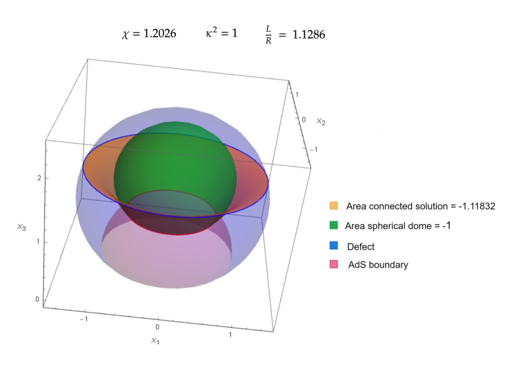
Figure 1: The projection of the minimal surface in AdS₅ is entirely contained in a sphere $S^{3}$ (see app. E). In this plot this sphere is mapped into $\mathds{R}^{3}$ through the usual stereographic projection. The blue spherical cap is the intersection between $S^{3}$ and the D5 while pink one is the intersection between $S^{3}$ and the boundary of AdS₅. Then the green dome and the yellow surface connecting the boundary with the D5 are the two competing solutions. For this choice of parameters the dominant solution is the connected one.

Nicely we recover, in the limit of large $k$, the result of Aguilera-Damia:2016bqv without restrictions on $L/R$ and $\chi$. The main output of our analysis is the discovery of a first-order phase transition of Gross-Ooguri type: for any flux $k$ and any non-zero angle $\chi$ the disk solution (describing the Wilson loop in the absence of defect) still exists and dominates, as expected, when the operator is far from the defect. On the other hand, our cylindrical string solution, connecting the boundary loop with the probe D5-brane, is favorite below a certain distance (or equivalently for a large radius of the circles). We can compare the classical actions associated with the solutions, by a mixture of analytical and numerical methods, finding the critical ratio $L/R$ as a function of $k$ and $\chi$. A related investigation has been performed in Preti:2017fhw for the quark-antiquark potential. A second important conclusion is that in the BPS case, that corresponds to $\chi=0$, the cylindrical solution does not exist for any choice of the physical parameters, suggesting that exchanges of light supergravity modes always saturate the expectation value at strong coupling. This behavior strongly resembles an analog result for correlators of relatively BPS Wilson loops in ${\cal N}=4$ SYM Drukker:2007qr , which can also be exactly computed through localization Giombi:2009ms ; Bassetto:2009rt . The weak coupling analysis corroborates the exceptionality of the BPS case: the first non-trivial perturbative contribution is evaluated exactly in terms of a Mejer-G function, and its large $k$ expansion does not scale in a way to match the string solution. In particular, it is not possible to recover the large $k$ limit starting from the equivalent asymptotic expansion of the $\chi\neq 0$ case: the order of limits does not commute. In the regime $L/R\to\infty$, we expect instead that the perturbative result could be understood in term of the OPE expansion of the Wilson loop: we confirm this idea, and we reconstruct the first two non-trivial terms of the expansion from the known results for the one-point function of scalar operators.

The structure of the paper is the following. In sec. 2 we start with discussing the generalities of the problem while in sec. 2.1 and sec. 2.2 we present the general solution of the equation of motions: we obtain an explicit expression for the functions $y(\sigma),r(\sigma),x_{3}(\sigma),\theta(\sigma)$ that describe the embedding of the string worldsheet into $AdS_{5}\times S^{5}$ ($\sigma$ is the spatial worldsheet parameter, see eqs. (2.14). and (2.15))

$$\begin{gathered}y(\sigma)=\frac{R\cosh\eta}{\sqrt{1+g^{2}(\sigma)}}\textrm{sech}[v(\sigma)-\eta]\quad\quad r(\sigma)=R\cosh\eta\frac{g(\sigma)}{\sqrt{1+g^{2}(\sigma)}}\textrm{sech}[v(\sigma)-\eta]\\ x_{3}(\sigma)=-R\cosh\eta\tanh[v(\sigma)-\eta]\quad\quad\theta(\sigma)=j\sigma+\chi.\end{gathered}$$ (1.1)

where the function $v(\sigma)$ is defined by

$$v^{\prime}(\sigma)=\sqrt{-\frac{\left(j^{2}+m\right)\left(j^{2}m+1\right)}{(m+1)^{2}}}\frac{1}{1+g^{2}(\sigma)},$$ (1.2)

and

$$\eta=v(\tilde{\sigma})+\tanh^{-1}\left(-\sqrt{-\frac{(m+1)^{2}}{\left(j^{2}+m\right)\left(j^{2}m+1\right)}}\frac{g^{\prime}(\tilde{\sigma})}{g(\tilde{\sigma})}\right).$$ (1.3)

The function $g(\sigma)$, that controls the full construction, has the explicit expression

$$g(\sigma)=\sqrt{\frac{j^{2}-1}{m+1}}\text{ns}\left(\sqrt{\frac{j^{2}-1}{m+1}}\sigma,m\right).$$ (1.4)

The minimal surface is given in terms of three real constants $(m,j,\tilde{\sigma})$ ($\tilde{\sigma}$ is the limiting value of the worldsheet coordinate) that are highly nonlinearly related to the physical parameters ($L/R,\chi,\kappa$) once the boundary conditions are imposed: we have defined $\kappa=\frac{\pi k}{\sqrt{\lambda}}$. Sec. 2.3 is devoted to finding the parameter space of the string solution, using the appropriate boundary conditions and some positivity requirements: the analysis can be performed restricting this moduli space into two regions that we call A and B (see equations (2.54)). In the limiting case $\chi=0$, both regions shrink to zero. Sec. 3 is the heart of our investigations, in which we discuss the structure of the connected string solution: the existence of the minimal surface is discussed as a function of the ratio $L/R$, and we find that there is a limiting value beyond that the solution ceases to exist. Moreover, there exist regions where a second branch appears, showing the presence of two competing connected solutions. For the sake of clarity, we display here the final result of this analysis, that singles out a critical angle, $\chi_{s}$, distinguishing two situations.

(1)

$\boldsymbol{\chi_{s}\leq\chi\leq\frac{\pi}{2}}$: In this case we have always two branches for the solution, no matter of the value of the flux $\kappa$

(2)

$\boldsymbol{0<\chi<\chi_{s}}$: In this region we can determine a critical value of the flux $\kappa_{s}(\chi)$: above this value we have a single branch solution while below a second branch appears.

The evaluation of the area of the minimal surface, obtained by computing the Polyakov action on the solutions is done in sec. 3.2. We find that the dominant branch is always physically connected to a vanishing distance from the defect. Finally in section 3.3 we compare the area of the dominant connected solution with the disk-like on-shell action: in the different regions we always find that decreasing $L/R$ from $+\infty$, where obviously the disk-like surface is the relevant saddle-point, there exists a critical value (depending on $(\chi,k)$) below which the connected cylinder starts being dominant. Nicely the disk solution (the spherical $dome$ as we will call it later) ceases to be dominant before touching the D5 brane profile. The last section is devoted to some perturbative computations, checking the picture emerging from strong coupling: first in sect. 4.1 we briefly recall the computation of the non-BPS Wilson loop at the first two perturbative orders and perform its double-scaling limit. Then in sect. 4.2 we explicitly expand in $\lambda/k^{2}$ the AdS/CFT solution. We recover the result of Aguilera-Damia:2016bqv without compromising ourselves with the value of other parameters (taking $L/R$ and $\chi$ generic) and showing the consistency with the relevant order of weak-coupling perturbation theory. Then we discuss the case $\chi=0$ in sec.4.3, remarking its peculiarity and highlighting the absence of a string counterpart. Finally, after having review the standard OPE expansion for the circular Wilson loop in sec. 4.4, we discuss the OPE picture of the present BPS case in sec. 4.5, finding consistency of our results with the known computations of some scalar one-point functions. Our conclusions and a list of interesting future follow-ups of our investigations are presented in sec. 5. A certain number of technical appendices complete the paper.

2 Prelude

The goal of the present paper is to study the vacuum expectation value of a circular Maldacena-Wilson loop in a four-dimensional dCFT given by $\mathcal{N}=4$ SYM theory with a co-dimension one hyperplane inserted at $x_{3}=0$ as in DeWolfe:2001pq ; Nagasaki:2011ue ; Buhl-Mortensen:2016jqo . More precisely, the defect separates two different $\mathcal{N}=4$ SYM theories: in the region $x_{3}<0$, we have the standard $\mathcal{N}=4$ SYM with gauge group $SU\left(N-k\right)$. On the other hand, an Higgsed $\mathcal{N}=4$ SYM lives in the $x_{3}>0$ region, with gauge group $SU\left(N\right)$, where three scalar fields receive a $x_{3}$-dependent VEV. At the level of the field theory, the picture is the following. The action for the dCFT is composed by two terms

$$S=S_{\mathcal{N}=4}+S_{D=3},$$ (2.1)

where $S_{\mathcal{N}=4}$ is the usual $\mathcal{N}=4$ SYM action that describes the bulk of the space-time, while $S_{D=3}$ accounts in general for degrees of freedom sited on the defect: they could both self-interact and couple to the bulk $\mathcal{N}=4$ SYM. The presence of the defect implies that fields living in the $x_{3}>0$ region will have a non-trivial vacuum solution: by imposing that a part of the supersymmetry is preserved a specific profile is obtained for the scalars. Following Nagasaki:2011ue , one assumes the ansatz

$$A_{\mu}=0\,\left(\mu=0,1,2,3\right),\qquad\Phi_{I}=\Phi_{I}(x_{3})\,\left(I,J,K=1,2,3\right),\qquad\Phi_{M}=0\,\left(M=4,5,6\right).$$ (2.2)

and the vanishing of fermions supersymmetry variation

$$0=\delta\psi=\partial_{3}\Phi_{I}\tilde{\Gamma}^{3I}\epsilon-\frac{i}{2}\left[\Phi_{I},\Phi_{J}\right]\tilde{\Gamma}^{IJ}\epsilon,$$ (2.3)

leads to the Nahm’s equations:

$$\partial_{3}\Phi_{I}=-\frac{i}{2}\epsilon_{IJK}\left[\Phi_{I},\Phi_{K}\right],$$ (2.4)

with $\epsilon$ satisfying

$$\left(1-\Gamma^{3456}\right)\epsilon=0.$$ (2.5)

We have followed the notation of Buhl-Mortensen:2016jqo and introduced $\tilde{\Gamma}^{I}=\Gamma^{I+3}$, $\tilde{\Gamma}^{3I}=\Gamma^{3}\Gamma^{I+3}$ and $\tilde{\Gamma}^{IJ}=\Gamma^{I+3}\Gamma^{J+3}$. The solution to eq. (2.4) it is known Constable:1999ac and it is called “fuzzy funnel” solution, reading

$$\left\langle\Phi_{I}\right\rangle_{\textrm{tree}}=\Phi_{I}^{\textrm{cl}}=-\frac{1}{x_{3}}t_{I}\oplus 0_{\left(N-k\right)\times\left(N-k\right)},$$ (2.6)

where $t_{I}$ are generators of a representation of $SU\left(2\right)$ (we can choose, for example, $I=1,2,3$). This means that the $t_{I}$ are $k\times k$ matrices satisfying

$$\left[t_{I},t_{J}\right]=i\epsilon_{IJK}t_{K},\qquad I,J,K=1,2,3.$$ (2.7)

All the other classical fields are zero. We observe that the $SO(6)$ R-symmetry of the original $\mathcal{N}=4$ SYM action is reduced to $SO(3)\times SO(3)$. We would like to study the expectation value of circular Maldacena-Wilson loops in this vacuum. A natural choice is to center the circle along the $x_{3}$ axis at a distance $L$ from the defect, i.e. $C=(0,0,0,L)$. The radius of the circle is $R$ and it extends only along the transverse directions $x_{1}$ and $x_{2}$, namely

$$x^{\mu}(\tau)=(0,R\cos\tau,R\sin\tau,L)$$ (2.8)

The residual $SO(3)\times SO(3)$ symmetry suggests to couple only two scalars to the Wilson loop: one massless $\Phi_{6}$ and one massive $\Phi_{3}$ and we get

$$\mathcal{W}=\mathrm{Pexp}\left(i\oint(A_{\mu}\dot{x}^{\mu}+i|\dot{x}|(\Phi_{3}\sin\chi+\Phi_{6}\cos\chi))\right),$$ (2.9)

where the angle $\chi$ parametrizes the strength of the coupling with the two scalars. Because of the conformal invariance $\langle\mathcal{W}\rangle$ does not depend separately by $L$ and $R$ but only through the ratio $R/L$. Moreover, the explicit analysis performed in Aguilera-Damia:2016bqv shows that in the absence of the defect our observable is always 1/2 BPS, but in its presence all the supercharges are broken unless $\chi=0.$

2.1 Setting-up the geometric description

On the string theory side, the field theory picture translates into a system of $N$ $D3-$branes intersecting a single $D5-$brane, where $k$ $D3-$branes out of the stack of $N$ terminate on it. In the near horizon limit we can view the D5 as a probe brane moving in $AdS^{5}\times S^{5}$. The intersection between D3 and D5 mimics the presence of a defect (domain wall) of codimension one located at $x_{3}=0$ in the field theory. The $AdS_{5}$ is is parametrized in Poincarè coordinates where the metric takes the form

$$ds^{2}_{AdS_{5}}=\frac{1}{y^{2}}(-dt^{2}+dy^{2}+dr^{2}+r^{2}d\phi^{2}+dx_{3}^{2}).$$ (2.10)

and for the sphere $S^{5}$ we write

$$ds^{2}=d\theta^{2}+\sin^{2}\theta d\Omega^{2}_{(1)}+\cos^{2}\theta d\Omega^{2}_{(2)},$$ (2.11)

where $d\Omega^{2}_{(i)}=d\alpha_{i}^{2}+\sin^{2}\alpha_{i}d\beta_{i}^{2}$ denotes the metric of the two $S^{2}$ inside the $S_{5}$. In these coordinates the $D5-$brane solution wraps the sphere $\Omega_{(1)}$ and its embedding in the target space is given by Nagasaki:2011ue

$$y=\frac{1}{\kappa}x_{3},\quad\quad\theta=\frac{\pi}{2},\quad\quad\alpha_{2}=\alpha^{(0)}_{2}\quad\quad\mathrm{and}\quad\quad\beta_{2}=\beta^{(0)}_{2},$$ (2.12)

where $\alpha_{2}^{(0)}$ and $\beta_{2}^{(0)}$ are two constant values. There is also an abelian background gauge field providing a non-trivial flux through $\Omega_{(1)}$, i.e.

$$\mathcal{F}=-\kappa~{}\mathrm{vol}(\Omega_{(1)}).$$ (2.13)

The coupling constant $\kappa$ in eq. (2.13) counts the unit of magnetic flux through the relation $\kappa=\frac{\pi k}{\sqrt{\lambda}}$.

For a single circular Wilson loop of radius $R$ (parallel to the defect) we expect to find two competing classical string solutions. One is the usual spherical dome anchored to the circle on the boundary of $AdS_{5}$,

$$y^{2}(\sigma)+r^{2}(\sigma)=R^{2}\ \ \ \ \ \ \ \ \ \phi=\tau,$$ (2.14)

which, however, does not move in the $S^{5}$. Alternatively, we can consider a second extremal surface stretching from the boundary to the D5-brane. This former is supposed to control the strong coupling behavior of this observable when $\frac{L}{R}\gg 1$, while the latter is expected to dominate the dynamics in the opposite regime, $\frac{L}{R}\ll 1$. To determine the second class of extremal surfaces, following Aguilera-Damia:2016bqv , we shall postulate the following ansatz

$$y=y(\sigma),\quad\quad r=r(\sigma),\quad\quad\phi=\tau,\quad\quad x_{3}=x_{3}(\sigma)\quad\mathrm{and}\quad\theta=\theta(\sigma),$$ (2.15)

for which the usual Polyakov action in conformal gauge reduces to

$$S=\frac{\sqrt{\lambda}}{4\pi}\int d\tau d\sigma\frac{1}{y^{2}}(y^{\prime 2}+r^{\prime 2}+r^{2}+x_{3}^{\prime 2}+y^{2}\theta^{\prime 2})$$ (2.16)

The Eulero-Lagrange equation of motion for the action (2.16) must be paired with the Virasoro constraint

$$y^{\prime 2}+r^{\prime 2}+x_{3}^{\prime 2}+y^{2}\theta^{\prime 2}=r^{2}.$$ (2.17)

At the boundary of $AdS_{5}$, which is approached when $\sigma\to 0$, the usual Dirichlet boundary conditions must be imposed:

$$y(0)=0,\quad\quad r(0)=R,\quad\quad x_{3}(0)=L\quad\mathrm{and}\quad\theta(0)=\chi.$$ (2.18)

We have also a second set of boundary conditions to be obeyed where the surface intersects the probe D5 brane. We must require that

$$C_{1}\equiv y(\tilde{\sigma})-\frac{1}{\kappa}x_{3}(\tilde{\sigma}) =0,\quad\quad\theta(\tilde{\sigma})=\frac{\pi}{2},$$ (2.19a)

$$C_{2}\equiv y^{\prime}(\tilde{\sigma})+{\kappa}x^{\prime}_{3}(\tilde{\sigma}) =0,\quad\quad C_{3}\equiv r^{\prime}(\tilde{\sigma})=0,$$ (2.19b)

where $\tilde{\sigma}$ is the maximum value of $\sigma$. Eqs. (2.19a) and (2.19b) simply state that extremal surface intersects orthogonally the boundary brane.

Since the coordinates $x_{3}$ and $\theta$ are ciclic variables in the action (2.16), their equations of motions immediately translate into two conservation laws

$$x_{3}^{\prime}(\sigma)=-cy^{2}(\sigma)\quad\quad\mathrm{and}\quad\quad\theta^{\prime}(\sigma)=j,$$ (2.20)

where $j$ and $c$ are two integration constants to be determined. The equations for $y(\sigma)$ and $r(\sigma)$ are instead

$$yy^{\prime\prime}+r^{\prime 2}+r^{2}-y^{\prime 2}+c^{2}y^{4}=0\quad\quad yr^{\prime\prime}-2r^{\prime}y^{\prime}-yr=0,$$ (2.21)

where we have used eqs. (2.20) to eliminate the dependence on $x_{3}$. The conservation laws eq. (2.20) also allow us to eliminate the dependence on $\theta$ and $x_{3}$ in the Virasoro constraint. We get

$${\cal V}(\sigma)\equiv\frac{r^{2}-y^{\prime 2}-r^{\prime 2}}{y^{2}}-c^{2}y^{2}=j^{2}.$$ (2.22)

2.2 General solution for the connected extremal surface

First we solve eq. (2.20) for $\theta$

$$\theta(\sigma)=j\sigma+\chi$$ (2.23)

where we used the b.c. $\theta(0)=\chi$. The second boundary conditions $\theta(\tilde{\sigma})=\frac{\pi}{2}$ determines the maximum value $\tilde{\sigma}$ of the world-sheet coordinate $\sigma$:

$$\tilde{\sigma}=\frac{1}{j}\left(\frac{\pi}{2}-\chi\right).$$ (2.24)

Next we focus our attention on the AdS radial coordinate $y(\sigma)$ and on $r(\sigma)$ which are determined by the system of coupled eqs. (2.21). To solve it we find convenient to introduce the auxiliary function $g(\sigma)\equiv\frac{r(\sigma)}{y(\sigma)}$. Then, with the help of eqs. (2.21) and of the Virasoro constraint $\mathcal{V}(\sigma)$, we find

$$\frac{g^{\prime\prime}(\sigma)}{g(\sigma)}=1-j^{2}+2g^{2}(\sigma),$$ (2.25)

a second order differential equation containing only $g(\sigma)$, which can be easily integrated to get the first integral

$$g^{\prime}(\sigma)^{2}+(j^{2}-1)g(\sigma)^{2}-g(\sigma)^{4}=-{\varepsilon_{0}}-j^{2},$$ (2.26)

where the arbitrary integration constant has been parameterized as $-{\varepsilon_{0}}-j^{2}$ for future convenience. This equation can be solved explicitly by quadratures through the method of separation of variables; but for the time being, we will not need the specific form of $g(\sigma)$.

To determine $y(\sigma)$, we can use the Virasoro constraint eq. (2.22) where we have eliminated $r(\sigma)$ in favor of $g(\sigma)$ and performed the change of variable

$$y(\sigma)=\frac{1}{\sqrt{1+g^{2}(\sigma)}z(\sigma)}.$$ (2.27)

We find that the unknown function $z(\sigma)$ satisfies the differential equation

$$\left(g^{2}(\sigma)+1\right)^{2}z^{\prime 2}(\sigma)-\varepsilon_{0}z^{2}(\sigma)+c^{2}=0.$$ (2.28)

Since the first and the last term in the l.h.s. of eq. (2.28) are strictly positive this equation can admit real solutions if and only if $\varepsilon_{0}\geq 0.$ We can now easily integrate eq. (2.28) by the method of separation of variables and get

$$z(\sigma)=\frac{c}{\sqrt{\varepsilon_{0}}}\cosh[v(\sigma)-\eta].$$ (2.29)

where the function $v(\sigma)$ is defined by

$$v^{\prime}(\sigma)=\frac{\sqrt{\varepsilon_{0}}}{1+g^{2}(\sigma)},$$ (2.30)

combined with the boundary condition $v(0)=0$. When deriving eq. (2.29) we have taken $c>0$ because $x_{3}(\sigma)$ must decrease while $\sigma$ grows (see eq. (2.20)). The parameter $\eta$ is an arbitrary integration constant. Then the expressions for the original coordinates ($y$ and $r$) in terms of $g(\sigma)$ and $v(\sigma)$ are given by

$$y(\sigma)=\frac{\sqrt{\varepsilon_{0}}}{c}\frac{1}{\sqrt{1+g^{2}(\sigma)}}\textrm{sech}[v(\sigma)-\eta]\quad\quad\mathrm{and}\quad\quad r(\sigma)=\frac{\sqrt{\varepsilon_{0}}}{c}\frac{g(\sigma)}{\sqrt{1+g^{2}(\sigma)}}\textrm{sech}[v(\sigma)-\eta].$$ (2.31)

Finally the coordinate $x_{3}$ is obtained by integrating eq. (2.20) with respect to $\sigma$. This can be done only in terms of the function $v(\sigma)$ and we obtain

$$x_{3}(\sigma)=x_{0}-\frac{\sqrt{\varepsilon_{0}}}{c}\tanh[v(\sigma)-\eta],$$ (2.32)

where $x_{0}$ is another arbitrary integration constant.

Next we can exploit the boundary conditions in $\sigma=0$ and $\sigma=\tilde{\sigma}$ to determine the different integration constants. Since $g(\sigma)\simeq 1/\sigma$ close to $\sigma=0$, the condition $r(0)=R$ becomes

$$\frac{\sqrt{\varepsilon_{0}}}{c}\textrm{sech}\eta=R\quad\quad\Rightarrow\quad\quad c=\frac{\sqrt{\varepsilon_{0}}}{R}\textrm{sech}\eta.$$ (2.33)

Instead $x_{3}(0)=L$ translates into

$$L=x_{0}+R\cosh\eta\tanh\eta\quad\quad\Rightarrow\quad\quad x_{0}=L-R\sinh\eta.$$ (2.34)

A suitable combination of the remaining three boundary conditions $C_{i}$ given in eq. (2.19) can be used to determine $\eta$ in terms of $L$:

$$0=\kappa cC_{1}+\frac{1}{y(\tilde{\sigma})}C_{2}+\frac{r(\tilde{\sigma})}{y^{2}(\tilde{\sigma})}C_{3}=c(R\sinh\eta-L)=0\quad\quad\Rightarrow\quad\quad\eta=\textrm{arcsinh}\frac{L}{R}.$$ (2.35)

Then we are left with two independent boundary conditions in $\sigma=\tilde{\sigma}$ to impose, for instance $C_{1}$ and $C_{3}$, which can be equivalently written as follows

$$\tanh\left(\eta-v\left(\tilde{\sigma}\right)\right)=\kappa\frac{\text{sech}\left(\eta-v\left(\tilde{\sigma}\right)\right)}{\sqrt{g^{2}\left(\tilde{\sigma}\right)+1}}\quad{\rm and}\quad\tanh\left(\eta-v\left(\tilde{\sigma}\right)\right)=-\frac{g^{\prime}\left(\tilde{\sigma}\right)}{\sqrt{\varepsilon_{0}}g\left(\tilde{\sigma}\right)}$$ (2.36)

The latter can be solved to determine $L/R$ as function of the two integration constant $j^{2}$ and $\epsilon_{0}$:

$$\textrm{arcsinh}\frac{L}{R}=\eta=v(\tilde{\sigma})+\tanh^{-1}\left(-\frac{1}{\sqrt{\varepsilon_{0}}}\frac{g^{\prime}(\tilde{\sigma})}{g(\tilde{\sigma})}\right).$$ (2.37)

Then the remaining boundary condition expresses the geometric flux $\kappa$ in terms of the same variables

$$\begin{split}\kappa=-\frac{g^{\prime}\left(\tilde{\sigma}\right)}{\sqrt{j^{2}+\epsilon_{0}-g^{2}\left(\tilde{\sigma}\right)}}.\end{split}$$ (2.38)

The solution of the boundary conditions can be used to simplify the form of the parametric representation eq. (2.31) and eq. (2.32) of the extremal surface. We find

$$\begin{gathered}y(\sigma)=\frac{R\cosh\eta}{\sqrt{1+g^{2}(\sigma)}}\textrm{sech}[v(\sigma)-\eta]\quad\quad r(\sigma)=R\cosh\eta\frac{g(\sigma)}{\sqrt{1+g^{2}(\sigma)}}\textrm{sech}[v(\sigma)-\eta]\\ x_{3}(\sigma)=-R\cosh\eta\tanh[v(\sigma)-\eta].\end{gathered}$$ (2.39)

Finally we can integrate eq. (2.26) to construct the explicit form of the function $g(\sigma)$:

$$g(\sigma)=\sqrt{\frac{j^{2}-1}{m+1}}\text{ns}\left(\sqrt{\frac{j^{2}-1}{m+1}}\sigma,m\right),$$ (2.40)

where

$$m\equiv\frac{j^{2}-1-\sqrt{\left(j^{2}+1\right)^{2}+4{\varepsilon_{0}}}}{j^{2}-1+\sqrt{\left(j^{2}+1\right)^{2}+4{\varepsilon_{0}}}}.$$ (2.41)

Since $\varepsilon_{0}>0$, the modular parameter $m$ is real and spans the interval $(-\infty,0]$. More specifically, from the definition eq. (2.41) we get two ranges for $m$ according the value of $j^{2}$:

$$(a):~{}-\infty<m<-1\quad{\rm and}\quad j^{2}<1\quad\quad(b):~{}-1\leq m\leq 0\quad{\rm and}\quad j^{2}\geq 1.$$ (2.42)

For $j^{2}=1$, we obtain $m=-1$ independently of the value of $\epsilon_{0}$. In the following we find more convenient to replace $\epsilon_{0}$ with $m$ as a free parameter by solving eq. (2.41). We get

$$\varepsilon_{0}=-\frac{\left(j^{2}+m\right)\left(j^{2}m+1\right)}{(m+1)^{2}}.$$ (2.43)

The positivity of the integration constant $\varepsilon_{0}$ combined with the bounds eq. (2.42) translates into the following ranges for the new couple of free parameters $(m,j^{2})$:

$$\mbox{\sc region (A):}~{}-1\leq m\leq 0~{}{\rm and}~{}j^{2}\geq-\frac{1}{m}\quad{\rm or}\quad\mbox{\sc region~{}(B):}~{}m\leq-1~{}{\rm and}~{}j^{2}\leq-\frac{1}{m}.$$ (2.44)

2.3 Allowed regions for the parameters ${j},{m}$

Since eq. (2.24) explicitly fixes $\tilde{\sigma}$ in terms of $j$ and $\chi$, the next step is to solve the highly non-linear system of equations (2.37) and (2.38) to determine the last two integration constants $m$ and $j$ as functions of $L/R,\chi$ and $\kappa$.

To begin with, we shall try to solve eq. (2.38) for $j$, or equivalently for the combination

$$x=\sqrt{\frac{j^{2}-1}{j^{2}(m+1)}},$$ (2.45)

as a function of $m,\kappa$ and $\chi$ . Since $\kappa=\frac{\pi k}{\sqrt{\lambda}}\geq 0$ and $g(\sigma)\geq 0$ (being the ratio of two positive coordinates), eq. (2.38) is solved for real values of the parameters if only if $g^{\prime}(\tilde{\sigma})<0$ and

$$g^{2}(\tilde{\sigma})\leq-m\frac{(j^{2}-1)^{2}}{(m+1)^{2}}$$ (2.46)

The bound (2.46) ensures that the quantity under the square root in the denominator of eq. (2.38) is non-negative. If we use eq. (2.40), the positivity of $g(\tilde{\sigma})$ and the requirement $g^{\prime}(\tilde{\sigma})<0$ can be translated into the following bounds for $\tilde{\sigma}=\frac{1}{j}\left(\frac{\pi}{2}-\chi\right)$

$$0\leq\tilde{\sigma}\leq\sqrt{\frac{m+1}{j^{2}-1}}\mathds{K}(m).$$ (2.47)

In terms of the auxiliary variable $x$ defined in eq. (2.45), they read

$$0\leq x\leq\frac{\mathds{K}\left(m\right)}{\left(\frac{\pi}{2}-\chi\right)}.$$ (2.48)

The bounds (2.44) for $j^{2}$ translate into $x\geq 1$ independently of the region. Thus the range of $x$ is given by

$$1\leq x\leq\frac{\mathds{K}\left(m\right)}{\left(\frac{\pi}{2}-\chi\right)}.$$ (2.49)

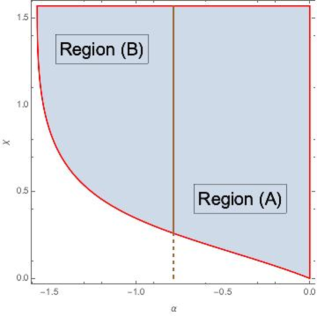
Figure 2: The light-blue region with the red boundary defines the allowed region in the $(\alpha,\chi)$-plane.

In the region (A) the variable $x$ is always less or equal to $\frac{1}{\sqrt{1+m}}$ by construction. Therefore, in this region, we can refine the bounds (2.49) as follows

$$1\leq x\leq\text{Min}\left(\frac{1}{\sqrt{1+m}},\frac{\mathds{K}\left(m\right)}{\left(\frac{\pi}{2}-\chi\right)}\right).$$ (2.50)

A necessary condition for the existence of solutions of eq. (2.38) is that the intervals (2.49) and (2.50) are not empty. We can solve this requirement numerically. If we set $m=\tan\alpha$ with $\alpha\in[-\frac{\pi}{2},0]$, the allowed region in the $(\alpha,\chi)$-plane is the light blue area in fig.2 bounded by the red line. The curved boundary is given by

$$\chi=\frac{\pi}{2}-\mathds{K}(m)=\frac{\pi}{2}-\mathds{K}(\tan\alpha),$$ (2.51)

namely the pairs $(\alpha,\chi)$ for which the intervals (2.49) and (2.50) collapses to a point.

In the above analysis we have neglected the constraint (2.46), which in terms of $x$ reads

$$\text{cn}^{2}\left(\left.x\left(\frac{\pi}{2}-\chi\right)\right|m\right)\leq-\frac{1}{m}\left(1-\frac{1}{x^{2}}\right).$$ (2.52)

This inequality implies the existence of stronger lower bound $x_{0}\geq 1$ for the unknown $x$. The value $x_{0}$ is defined as the value that saturates the inequality (2.52), i.e.

$$-m\text{cn}^{2}\left(\left.x_{0}\left(\frac{\pi}{2}-\chi\right)\right|m\right)=1-\frac{1}{x_{0}^{2}},$$ (2.53)

and respects the bounds (2.50) in region (A) and (2.49) in region (B). Summarizing, we have the following two ranges for $x$

$$\mbox{\sc region (A):}\quad x_{0}\leq x\leq\text{Min}\left(\frac{1}{\sqrt{1+m}},\frac{\mathds{K}\left(m\right)}{\left(\frac{\pi}{2}-\chi\right)}\right)\quad\mbox{\sc region~{}(B):}\quad x_{0}\leq x\leq\frac{\mathds{K}\left(m\right)}{\left(\frac{\pi}{2}-\chi\right)}.$$ (2.54)

However the new bounds for $x$ does not alter the allowed region in the $(\alpha,\chi)-$plane in fig. 2.

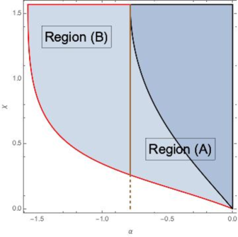
Figure 3: The inequality (2.55) holds in the light-blue region on the left of the black-line.

Next we shall analyze how the value of the flux $\kappa$ may change (in particular reduce) the allowed region. Given $m$ and $\chi$, eq. (2.38) is solved for $\kappa=0$ if we take $x=\frac{\mathds{K}\left(m\right)}{\frac{\pi}{2}-\chi}$ (namely the value for which $g^{\prime}(\tilde{\sigma})=0$). However, in the region (A) this $x$ is an acceptable solution if and only if

$$\frac{\mathds{K}\left(m\right)}{\frac{\pi}{2}-\chi}\leq\frac{1}{\sqrt{1+m}}.$$ (2.55)

The inequality (2.55) is obeyed in the ligth-blue region on the left of the black curve in fig. 3. In the darker region on the right of the black curve we cannot solve eq. (2.38) for arbitrary small value of $\kappa.$

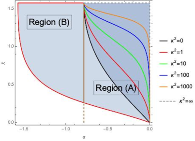
Figure 4: The coloured curves inside the darker region correspond to different values of $\kappa^{2}$ . The allowed region for $m$ for fixed value of $\kappa^{2}$ is the one on the left of the relevant coloured curve. The region becomes larger when we increase the flux.

We can equivalently reformulate this obstruction as follows. We fix the flux $\kappa$ and the angle $\chi$ and we increase $m$ starting from its lower bound $-1$ in the region (A). We will reach a critical value $m_{c}$ such that eq. (2.38) is solved by the largest acceptable value for $x$, i.e. $x_{c}=\frac{1}{\sqrt{1+m_{c}}}$. Then, for $m\geq m_{c}$, there is no solution of eq. (2.38) in the interval (2.54). Therefore, given $\kappa$ and $\chi$, the set of allowed parameters is further restricted by the requirement the l.h.s. of (2.38) must be less than $\kappa$ when $x=\frac{1}{\sqrt{1+m}}$:

$$\text{sn}\left(\frac{(\pi-2\chi)}{2\sqrt{m+1}}|m\right)\geq\frac{\sqrt{2}}{\sqrt{m+1+\sqrt{(m-1)^{2}-4m\kappa^{2}}}},$$ (2.56)

$m_{c}$ is the value of $m$ that saturates the inequality (2.56). In fig. 4 we have plotted the curve defined by the equality in eq. (2.56) for different values of $\kappa$. Given a specific value of $\kappa$, the allowed region is the ligth-blue one on the left of the corresponding curve. This region increases when $\kappa$ grows and we recover the entire region (A) when $\kappa=\infty.$

The critical value $m_{c}$ possesses a simple geometrical interpretation. In fact we can easily check that the distance $L/R=\sinh\eta$ vanishes as $m\to m_{c}$ (see sec. 3.1), namely the Wilson loop touches the defect at $m=m_{c}$ and the solution stops to exist.

The red curve in fig. 4, which is the exterior boundary of the allowed region, corresponds to $m=-1/j^{2}$, i.e. to $c=0$. For this particular choice of the parameters, our solutions coincide with the ones previously discussed in Aguilera-Damia:2016bqv . In fact our functions simplifies to

$$\begin{split}g(\sigma)=&j~{}\text{ns}\left(j\sigma\left|-\frac{1}{j^{2}}\right.\right)=\\ =&\sqrt{1+j^{2}}\text{ds}\left(\left.\sqrt{1+j^{2}}\sigma\right|\frac{1}{1+j^{2}}\right)\end{split}$$ (2.57)

and

$$\begin{split}h(\sigma)=&\frac{1}{R}g(\sigma)\sqrt{1+\frac{1}{g(\sigma)^{2}}}=\frac{\sqrt{1+j^{2}}}{R}\text{ns}\left(\sqrt{1+j^{2}}\sigma\left|\frac{1}{1+j^{2}}\right.\right),\end{split}$$ (2.58)

where we use the modular properties of the elliptic trigonometric functions. The solutions (2.57) and (2.58) are easily seen to be identical to the ones constructed in Aguilera-Damia:2016bqv .

Some specific comments are in order for the two extremal points $\chi=0$ (BPS configuration) and $\chi=\frac{\pi}{2}$.

$\chi=0$ case:

For this choice of the angle governing the coupling of the scalars, the admissible region for $m$ shrinks to a point, $m=0$ (see fig. 4). Consequently the integration constant $j^{2}$, which must be always greater than $-1/m$, diverges and $\tilde{\sigma}=\frac{\pi}{2j}$ vanishes. In other words, the space of parameters collapses to a point and no regular connected solution exists for the BPS configuration.

$\chi=\frac{\pi}{2}$ case:

The case $\chi=\frac{\pi}{2}$ will be discussed in details in sec. D. At variance with the other values of $\chi$ the disconnected solution cannot exist for all distances: in fact when $\frac{L}{\kappa R}=1$ the disconnected solution touches the brane. If this would happen before the connected solution starts dominating, the phase transition from the disconnected to the connected solution would become of order $0$.

3 The structure of the solutions

3.1 The distance from the defect

Once we solved eq. (2.38) to obtain $x$ (and thus $j$) in terms of $\chi,\kappa$ and $m$, the distance from the defect can be computed through eq. (2.37). An analytic expression of this quantity in terms of elliptic integral of the third kind is given in appendix A.

The goal of this section is to determine when we can invert eq. (2.37) and determine the last integration constant $m$ as a function of the dimensionless distance $L/R$, $\chi$ and $\kappa$. If we keep fixed the last two quantities, the dependence of $\frac{L}{R}=\sinh\eta$ on $m$ is monotonic (and thus invertible) if $\frac{\partial\eta}{\partial m}$ does not change sign. We can obtain a compact expression for this derivatives in two steps. First we take the derivative of eq. (A) with respect to $m$: the final result contains a pletora of elliptic trigonometric functions and second elliptic integrals $\mathds{E}(\sqrt{n}\tilde{\sigma},m)$. We can eliminate the last dependence by exploiting the derivative of eq. (2.38) for the flux. The final expression is relatively simple

$$\left.\frac{\partial\eta}{\partial m}\right|_{\chi,\kappa}=\frac{\left[\frac{n^{2}(n+1)\left(mn+1\right)}{1-m}-m\left(1-m\right)\left(\partial_{m}n-\frac{n(n+1)}{1-m}\right)^{2}\right]\left(\frac{2g(\tilde{\sigma})g^{\prime}(\tilde{\sigma})}{2mn^{2}g(\tilde{\sigma})^{2}+g(\tilde{\sigma})^{4}-mj^{2}n^{2}}+\frac{\pi-2\chi}{j^{3}}\right)}{4n\sqrt{-(n+1)\left(mn+1\right)}},$$ (3.1)

where the derivative is taken at constant $\chi$ and $\kappa$ and

$$n\equiv\frac{j^{2}-1}{m+1}.$$ (3.2)

In eq. (3.1) $\partial_{m}n$ denotes the derivative of $n$ with respect to $m$. It is not difficult to check that the second factor in eq. (3.1) is always positive in the range $n\leq g^{2}(\sigma)\leq-mn^{2}$. Thus the sign of eq. (3.1) is entirely controlled by the factor between square brackets.

In subsec. 2.3, we argued that we can find a value $m_{c}$ of $m$ such that no solution exists for $m>m_{c}$ for fixed $\chi$ and $\kappa$. This critical value $m_{c}$ solves (see eq. (2.56))

$$\text{sn}\left(\frac{(\pi-2\chi)}{2\sqrt{m_{c}+1}}|m_{c}\right)=\frac{\sqrt{2}}{\sqrt{m_{c}+1+\sqrt{(m_{c}-1)^{2}-4m_{c}\kappa^{2}}}}.$$ (3.3)

We can now easily expand $n$ around $m_{c}$ and at the leading order we find

$$n=\frac{x^{2}}{1-(m+1)x^{2}}=\frac{c_{0}}{m_{c}-m}+O(1)\ \ \ \ \mathrm{with}\ \ \ \ 0<c_{0}<1,$$ (3.4)

namely $n$ blows up at $m=m_{c}$. The bounds on the constant $c_{0}$ are equivalent to the fact that $x$ decreases for $m<m_{c}$. The combination $\sqrt{n}\tilde{\sigma}$ is instead finite when $m$ approaches $m_{c}$ (i.e. $\sqrt{n}\tilde{\sigma}\mapsto\frac{\pi-2\chi}{2\sqrt{1+m_{c}}}$). In this limit it is quite straightforward to show that $\eta$ vanishes. In fact the argument of $\tanh^{-1}$ in eq. (2.37) behaves as $1/\sqrt{n}$, while $v(\tilde{\sigma})$ vanishes as $1/\sqrt{n}$ (see appendix A).

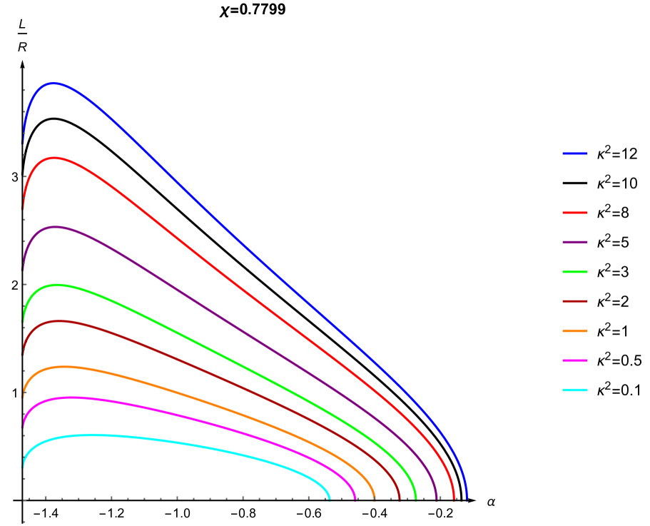
(a)

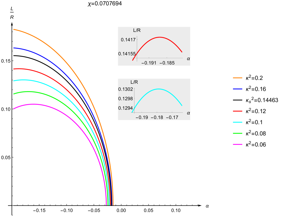
(b)

Figure 5: We have plotted the distance $L$ as a function of $\alpha=\arctan(m)$. In (a) we have chosen an angle $\chi>\chi_{s}$: the different curves corresponds to different values of the flux. All the curves display a maximum. In (b) we have chosen an $\chi<\chi_{s}$. When we are above the critical flux $\kappa>\kappa_{s}$ (the black curve), the curves are monotonic. On the contrary, as $\kappa$ becomes smaller than $\kappa_{s}$ (i.e. we are below the black curve) again a maximum appears.

If we use the above behavior of $n$ close to $m_{c}$, we can also check that the derivative of $\eta$ in $m_{c}$ and thus of the distance diverges to $-\infty$ as $\sqrt{n}$. This is consistent with the behavior of the curves plotted in fig. 5. When we decrease $m$ the parameter $\eta$ increases, i.e. we are moving away from the brane. To understand if this behavior takes place for all the range spanned by $m$ at fixed $\kappa$ and $\chi$, we shall investigate the sign of $\frac{\partial\eta}{\partial m}$ when we reach the other boundary of the allowed region, namely the red curve in fig. 2. The value $m_{0}$ lying on this second boundary is determined only by the angle $\chi$ and it satisfies

$$\chi=\frac{\pi}{2}-\mathds{K}(m_{0}).$$ (3.5)

Then the derivative of $\eta$ with respect to $m$ computed at $m=m_{0}$ is given by (see app. B for a derivation of this result)

$$\begin{split}\left.\frac{\partial\eta}{\partial m}\right|_{m=m_{0}}=&\frac{\left(1-m_{0}\right)\left(\mathds{E}\left(m_{0}\right)+(m_{0}-1)\mathds{K}\left(m_{0}\right)\right){}^{2}+m_{0}\kappa^{2}\left(1-\left(\mathds{E}\left(m_{0}\right)+\left(m_{0}-1\right)\mathds{K}\left(m_{0}\right)\right){}^{2}\right)}{2\kappa\left(1-m_{0}\right)\left(-m_{0}\right){}^{3/2}\sqrt{1-\left(\kappa^{2}+1\right)m_{0}}}\end{split}$$ (3.6)

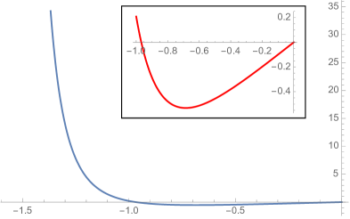
Figure 6: Plot of the coefficient of $\kappa^{2}$ in the numerator of eq. (3.6) [we have set $m_{0}=\tan\alpha\ \textrm{with}\ \alpha\in(-\pi/2,0]$]. It is negative between zero and and a critical value $m_{s}=\tan\alpha_{s}=-1.45221$. For $m<m_{s}$ the coefficient is always positive.

The sign of this quantity is controlled by the sign of the coefficient of the term linear in $\kappa^{2}$ in the numerator of eq. (3.6) since the other term is manifestly positive for negative values of $m_{0}$. In fig. 6 we have plotted the coefficient of $\kappa^{2}$. We recognize that there is a critical value $m_{s}\simeq-1.45221$ for which this coefficient vanishes, namely

$$\left(m_{s}-1\right)\mathds{K}\left(m_{s}\right)+\mathds{E}\left(m_{s}\right)+1=0.$$ (3.7)

We can translate $m_{s}$ into an equivalent critical angle $\chi_{s}=\frac{\pi}{2}-\mathds{K}(m_{s})\simeq 0.331147$. The angle $\chi_{s}$ separates two distinct regions of parameters:

(1):

$\mathbf{m_{0}\boldsymbol{\leq}m_{s}}\ \textrm{(or}\ \boldsymbol{\chi_{s}\leq\chi\leq\frac{\pi}{2}}$). The coefficient of $\kappa^{2}$ and thus the derivative in $m=m_{0}$ are positive independently of the value of the flux. Since the same derivative diverges to $-\infty$ on the other extremum of the interval $m=m_{c}$, the dependence of $\eta$ on $m$ cannot be monotonic and we cannot invert eq. (2.37) on the entire range of the allowed $m^{\prime}$s. In fact, as illustrated in fig. 5 (a), when we decrease $m$ starting from the value $m_{c}$ defined by eq. (3.3) the distance from the brane starts increasing, it reaches a maximum and then decreases to the value reached for $m=m_{0}$.

(2):

$\mathbf{m_{s}\boldsymbol{<}m_{0}<0}\ \textrm{(or}\ \boldsymbol{0<\chi<\chi_{s}}).$ The derivative of $\eta$ with respect to $m$ computed at $m=m_{0}$ is always negative unless the flux $\kappa^{2}$ is below a the critical value $\kappa_{s}^{2}$ given by

$$\kappa_{s}^{2}=\frac{m_{0}-1}{m_{0}\left(\frac{1}{\left(\left(m_{0}-1\right)K\left(m_{0}\right)+E\left(m_{0}\right)\right){}^{2}}-1\right)}.$$ (3.8)

We find more instructive to view this critical flux $\kappa_{s}^{2}$ defined in eq. (3.8) as a function of the angle $\chi$ (instead of $m_{0}$) by exploiting eq. (3.5). If we draw the curve $\kappa_{s}^{2}(\chi)$ we obtain the blue curve in fig. 7. Given the angle $\chi$ (with $0<\chi<\chi_{s}$) we can determine a critical value of the flux $\kappa_{s}$ by means of the plot 7. The black curve in fig. 5 (b) displays the behavior of the distance with $m$ for the critical value of the flux: it is monotonic and has vanishing derivative at $m=m_{0}$. If we choose a flux greater than $\kappa_{s}$ (the curves above the black one), the distance is a monotonic function of $m$, namely its derivative never vanishes. Below this critical value of the flux (i.e. the curves below the black one) the derivatives vanishes just once: namely when we decrease $m$ starting from the value $m_{c}$ the distance starts increasing, it reaches a maximum and then decreases to the value reached for $m=m_{0}$.

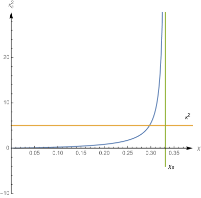
Figure 7: The blue curve illustrates the behavior of the critical flux in the interval $[0,\chi_{s}]$, where it exists. It is a monotonic function of $\chi$ and it ranges from $0$ to $\infty$.

The presence of a non-monotonic behavior (for a certain range of parameters) is synonymous of the existence of different branches of solutions. In other words, if either $\chi_{s}\leq\chi\leq\frac{\pi}{2}$ or $0<\chi<\chi_{s}$ and $\kappa^{2}<\kappa_{s}^{2}$, we can find value of the distance for which we can construct two different extremal connected surfaces. We shall come back to this point when we discuss the area of the extremal surfaces.

In both regions ((1) and (2)) there exists a maximal distance $L_{\rm\tiny max}$ after which the connected solution stops to exist. When $0<\chi<\chi_{s}$ and we are above the critical flux $\kappa_{s}$, $L_{\rm\tiny max}$ is obtained when we reach the boundary $m=m_{0}$. since we are considering the range of parameters for which distance is a monotonic function of $m$. If we use the expansion in App. B and substitute into eq. (A) we find

$$\eta_{\max}=\tanh^{-1}\sqrt{\frac{\kappa^{2}m_{0}}{\kappa^{2}m_{0}+m_{0}-1}}\ \ \ \ \ \Rightarrow\ \ \ \ \ \ \ L_{\rm\tiny max}=R\sinh\eta_{\tiny\rm max}=R\sqrt{\frac{\kappa^{2}m_{0}}{m_{0}-1}}$$ (3.9)

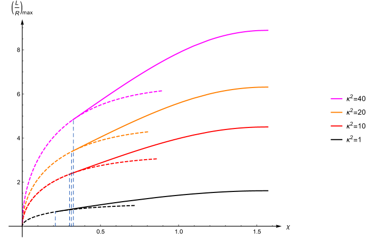
Figure 8: The dashed curves are given by eq. (3.9) describe the distance for $\chi<\chi_{\kappa^{2}}$ while the continuous ones are valid for $\chi>\chi_{\kappa^{2}}$. Different colors corresponds to different fluxes. We see the maximal distance grows both with $\chi$ and $\kappa^{2}$. We have drawn the dashed curves also for values greater than $\chi_{\kappa^{2}}$ to show that the merging of the two branches is continuous with its first derivative.

If we are below the critical flux or the angle $\chi$ is in the range $(\chi_{s},\frac{\pi}{2})$ the maximal distance from the brane cannot be determined analytically, but only numerically. In fig. 8 we have plotted this quantity as a function of $\chi$ for different values of the flux $\kappa^{2}$. Given $\kappa^{2}$, we can always find an angle $\chi_{\kappa^{2}}\in[0,\chi_{s}]$ for which $\kappa^{2}$ is exactly the critical flux (see fig. 7). For angles in the interval $[0,\chi_{\kappa^{2}})$, the maximal distance is given by eq. (3.9) and is represented by the dashed curves in fig. 8. For angles greater than $\chi_{\kappa^{2}}$, the behavior of the distance is described by the continuous lines in fig. 8. The merge of the two branches of the distance (dashed and continuous) is continuous with its first derivative as one can show by a direct computation of the left and right derivative in $\chi_{\kappa^{2}}$. In fig. 8, we have drawn the dashed curves also for values greater than $\chi_{\kappa^{2}}$ to illustrate that two branches are not given by the same function.

The general behavior of the distance displayed in fig. 8 is easily summarized: the maximal distance increases with $\chi$ at fixed $\kappa^{2}$ and increases with $\kappa^{2}$ at fixed angle, The latter behavior is expected: in fact, when $\kappa^{2}$ grows the slope of the brane becomes smaller and smaller and the brane is closer to the boundary. Therefore the cost in energy (in area) is low for a larger interval of the distances.

3.2 The Area

The regularized area of the connected minimal surfaces is obtained by evaluating the Polyakov action on the classical solution $(r(\sigma),y(\sigma))$:

$$\mathcal{S}=\frac{\sqrt{\lambda}}{4\pi}\int d\tau d\sigma\frac{1}{y^{2}}(y^{\prime 2}+r^{\prime 2}+r^{2}+c^{2}y^{4}+j^{2}y^{2}).$$ (3.10)

We can eliminate the explicit dependence on the integration constants $j$ and $c$ by means of the Virasoro constraint (2.22). We find

$$S=\frac{\sqrt{\lambda}}{4\pi}\int_{\Sigma}d\tau d\sigma\frac{1}{y^{2}}(y^{\prime 2}+r^{\prime 2}+r^{2}+r^{2}-y^{\prime 2}-r^{\prime 2})={\sqrt{\lambda}}\int_{{\sigma_{\epsilon}}}^{\tilde{\sigma}}d\sigma\frac{r^{2}(\sigma)}{y^{2}(\sigma)}={\sqrt{\lambda}}\int_{{\sigma_{\epsilon}}}^{\tilde{\sigma}}d\sigma g^{2}(\sigma),$$ (3.11)

where we have used that the integrand does not depend on $\tau$ to perform the integration over this world-sheet coordinate. Remarkably the area depends only on the function $g(\sigma)$. The integration over $\sigma$ runs from $\sigma_{\epsilon}$, the value of $\sigma$ for which the minimal surface intersects the plane $y=\epsilon$, to $\tilde{\sigma}$, the value of $\sigma$ for which the minimal surface intersects the boundary brane. The lower extremum $\sigma_{\epsilon}$ is determined by solving $y(\sigma_{\epsilon})=\epsilon$ for small $\epsilon$. At the lowest orders in $\epsilon$ we find the following expansion:

$$\sigma_{\epsilon}=\frac{\epsilon}{R}+\frac{1}{6}(j^{2}+2)\frac{\epsilon^{3}}{R^{3}}+O(\epsilon^{4}).$$

Next we can easily perform the integration over the coordinate $\sigma$ in terms of elliptic integral of the second kind and we get

$$\mathcal{S}_{\epsilon}=\left.\sqrt{\lambda n}\left(\sqrt{n}\sigma-\mathds{E}\left(\text{am}\left(\sqrt{n}\sigma|m\right)|m\right)-\frac{\text{cn}\left(\sqrt{n}\sigma|m\right)\text{dn}\left(\sqrt{n}\sigma|m\right)}{\text{sn}\left(\sqrt{n}\sigma|m\right)}\right)\right|_{\sigma_{\epsilon}}^{\tilde{\sigma}}.$$ (3.12)

The expected ultraviolet linear divergence arises when we evaluate the primitive in the lower extremum. Since the term $\epsilon^{2}$ is absent in the expansion of $\sigma_{\epsilon}$, the lower extremum does not give any non-vanishing contribution in the limit $\epsilon\to 0$. The only contribution to the renormalized area originates from the upper extremum:

$$\mathcal{S}_{\rm ren.}=\sqrt{\lambda n}\left(\sqrt{n}\tilde{\sigma}-\mathds{E}\left(\text{am}\left(\sqrt{n}\tilde{\sigma}|m\right)|m\right)-\frac{\text{cn}\left(\sqrt{n}\tilde{\sigma}|m\right)\text{dn}\left(\sqrt{n}\tilde{\sigma}|m\right)}{\text{sn}\left(\sqrt{n}\tilde{\sigma}|m\right)}\right)\equiv\sqrt{\lambda}\mathcal{\hat{S}}_{\rm ren.}.$$ (3.13)

The behavior of the renormalized action as a function of the distance from the defect can be investigated by computing its derivative with respect to $m$ at fixed $\kappa$ and $\chi$. We proceed by following the same two steps performed for the evaluation of $\left.\frac{\partial\eta}{\partial m}\right|_{\kappa,\chi}$ and we get the remarkable identity

$$\left.\frac{\partial\hat{\mathcal{S}}_{\rm ren.}}{\partial m}\right|_{\kappa,\chi}=\sqrt{-(n+1)(mn+1)}~{}\left.\frac{\partial\eta}{\partial m}\right|_{\kappa,\chi}$$ (3.14)

namely the derivative of the action and of $\eta-$parameter (the distance) are proportional through a positive definite factor. Thus the derivative of the $\hat{\mathcal{S}}_{\rm ren.}$ with respect to $\eta$ or equivalently to $L$ has a very simple form

$$\left.\frac{\partial\hat{\mathcal{S}}_{\rm ren.}}{\partial L}\right|_{\kappa,\chi}=\frac{1}{R\sqrt{1+\frac{L^{2}}{R^{2}}}}\left.\frac{\partial\hat{\mathcal{S}}_{\rm ren.}}{\partial\eta}\right|_{\kappa,\chi}=\frac{\sqrt{-(n+1)(mn+1)}}{R\sqrt{1+\frac{L^{2}}{R^{2}}}}=c(L,\kappa,\chi)$$ (3.15)

where $c$ is the integration constant appearing in eq. (2.20) for $x_{3}$. A similar relation was found in Kim:2001td for the potential quark-antiquark at finite temperature. There it was speculated that this kind of relation might enjoy some sort of universality.

Because of eq. (3.14) the area and the distance possess the same behavior as functions of $m$:

• $\boldsymbol{\chi_{s}\leq\chi\leq\frac{\pi}{2}}$ or $\boldsymbol{0<\chi<\chi_{s}}$ and $\boldsymbol{\kappa\leq\kappa_{s}}$: when we move away from the D$5$-brane by decreasing $m$ from its critical value $m_{c}$ (corresponding to vanishing distance) both the area and the distance increase and reach their maximum value for the same value of $m$. Then both decrease up to $m=m_{0}$ (i.e. the curved red boundary in fig. 3).

• $\boldsymbol{0<\chi<\chi_{s}}$ and $\boldsymbol{\kappa>\kappa_{s}}$: both the area and the distance monotonically increase when $m$ is lowered from $m_{c}$ to $m_{0}$.

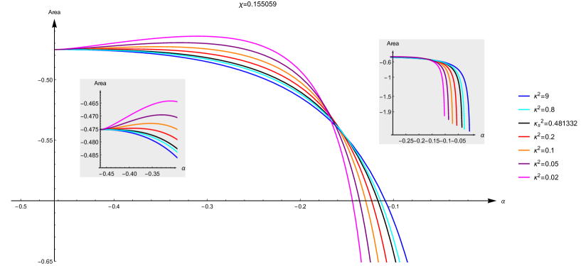
Figure 9: We have plotted the behaviour of the area as a function of $\alpha=\arctan(m)$ for a fixed value of the angle $\chi$ (below $\chi_{s}$) but for different values of the flux. On the left we have zoomed the region close to the red curved boundary in fig. 2. Independently of $\kappa^{2}$ all the curves terminate on the same point ($m_{0},\chi_{0}=\frac{\pi}{2}-\mathds{K}(m_{0})$). For values of $\kappa^{2}\leq\kappa^{2}_{s}$, this curve displays a maximum, instead they are monotonic if we are above the critical flux $\kappa_{s}$. On the right we have plotted the same curves in the region close to $m_{c}=\tan\alpha_{c}$, namely the value for which the distance from the brane vanishes. The area diverges for all value of the flux.

In fig. 9 we have plotted the area as a function of $\alpha\equiv\arctan(m)$ for a fixed angle $\chi=0.155059$ in the range $0<\chi<\chi_{s}$. On the left gray box we have zoomed on the behavior of the area for different value of the flux in the proximity of the value $m_{0}$ on the curved red boundary in fig. 2. Below the critical value of the flux (black curve) determined by eq.(3.8) all the lines possess a maximum, while above $\kappa^{2}_{s}$ they are monotonically decreasing. However, independently of the flux, all of them terminate in the same point since the boundary value on the red curve in fig. 2 does not depend on the flux. On the right gray box we have zoomed in the region close to the brane, the action always diverges when $m$ approaches the values $m_{c}$, obtained by solving eq. (3.3).

The typical behavior of the area in the region $\chi_{s}\leq\chi\leq\frac{\pi}{2}$ as function of $m$ is displayed in fig. 10. Independently of $\kappa^{2}$ all the curves terminate on the same point ($m_{0},\chi_{0}=\frac{\pi}{2}-\mathds{K}(m_{0})$) and possess a maximum for the same value of $m$ for which the distance does (see left gray box).

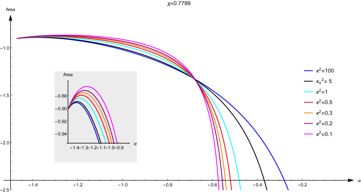
Figure 10: We have plotted the behaviour of the area as a function of $\alpha=\arctan(m)$ for a value of the angle above $\chi_{s}$ and for different values of the flux. Independently of $\kappa^{2}$ all the curves terminate on the same point ($m_{0},\chi_{0}=\frac{\pi}{2}-\mathds{K}(m_{0})$) and display a maximum. On the left we have zoomed in the region close to $m_{0}$ to show the presence of a maximum value for the area.

We conclude this section with an amusing observation about the derivatives of the area with respect the two other parameters. It is not difficult to check that both of them can be rewritten in terms of the same derivative of $\eta$:

$$(A_{1}):\ \ \frac{\partial\mathcal{A}}{\partial\chi}=\sqrt{-(n+1)(mn+1)}~{}\frac{\partial\eta}{\partial\chi}-j\qquad(A_{2}):\ \ \kappa\frac{\partial\mathcal{A}}{\partial\kappa}=\sqrt{-(n+1)(mn+1)}~{}\kappa\frac{\partial\eta}{\partial\kappa}+\frac{g^{\prime}(\tilde{\sigma})}{g(\tilde{\sigma})}$$ (3.16)

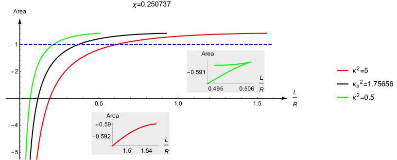
Figure 11: This graphic displays the behavior of the area as a function of the distance $L/R$ for a fixed value of the angle $\chi=0.250737<\chi_{s}$. In this range there is a critical flux $\kappa_{s}^{2}=1.75656$ and the area for this value of the flux is the black curve. Above the critical flux, the typical behavior is given by the red curve, namely the area is a monotonic function of the distance and the solution stops existing after a maximal value of the distance. Below the critical flux, the typical behavior is instead described by the green curve. There are two branches of solutions. However the upper one is always subdominant. In this plot we normalized the area functional so that the area of the dome is $-1$.

3.3 Transition: connected solution vs dome

To understand when the connected solution becomes dominant with respect to the spherical dome we have to plot the area as a function of the distance from the brane. This can be done by exploiting the result of the previous two sections. We have to distinguish two cases depending on the angle $\chi$ governing the coupling with the scalars:

$\boldsymbol{0<\chi<\chi_{s}}$:

Above the critical flux $\kappa_{s}$ (represented by the black curve in fig. 11) the area is a monotonic function of the distance (see e.g. the red curve in fig. 11). If we are approaching from infinity the connected solution start to exist at certain maximal distance, which depends on $\chi$ and is given by eq. (3.9). The area is larger than the one of the dome, which, therefore, still dominates. While we are getting closer the area keeps decreasing and we reach a critical distance where the connected solution and the disconnected one have the same area. In fig. 11 the critical distance is realized when the red curve crosses the blue line. After this value of the distance, the connected solution becomes the dominant one: in fact the area keeps decreasing and diverges to $-\infty$ when we reach the brane.

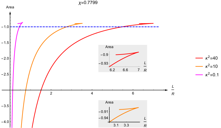
Figure 12: This plot displays the behavior of the area as a function of the distance $L/R$ for a fixed value of the angle $\chi=0.7799>\chi_{s}$. In this range there is no critical flux. The typical behavior is described by the three curves (red, orange and purple). There are always two branches of solutions. However the upper one is always subdominant. In this plot we normalized the area functional so that the area of the dome is $-1$.

The typical behavior of the area below the critical flux $\kappa_{s}$ is described, instead, by the green curve in fig. 11. There is still a maximal distance, at which the connected solution starts to exist, but when the distance decreases there are two different branches of solutions: namely we have two connected extremal surfaces with the same angle $\chi$, flux $\kappa$ and distance $L$. In fig. 11, this is clearly displayed in the zoom of the region close to the maximal distance. The upper branch corresponds to the values of the modular parameter $m$ ranging from $m_{0}$, lying on the red curved boundary in fig. 2, to the value corresponding to the maximal distance. The lower one is instead obtained when $m$ runs from the value corresponding to the maximal distance to $m_{c}$, for which the distance from the brane vanishes. The area of the solution in the upper branch, when it exists, is always subdominant with respect to the one in the lower branch. Therefore, we can focus on the latter.

$\boldsymbol{\chi_{s}\leq\chi\leq\frac{\pi}{2}}$:

The behavior of the area as function of the distance in this range of angles is displayed in fig. 12. The situation is analogous to what occurs in the other region below the critical flux. Starting from the maximal distance for which the connected solution exists, we have two families of extremal surfaces when the distance decreases. However, as we can see in in fig. 12, the shorter one is always subdominant. The one relevant for us will be the lower branch running from the maximal distance to the brane. The length of the subdominant branch increases with the flux.

In both regions there is always a value of the distance for which the area of the dome is equal to the area of the connected solution and below which the connected solution becomes dominant. In other words we have a phase transition. In fact above this critical distance, the dominant solution is the spherical dome and the area is constant (the dashed blue line in fig. 11 and 12). The transition is of the first order since the area is continuous but not its first derivative. The critical distance increases with the flux, as one expects.

In fig. 13, we have drawn the critical surface in the parameter space $(\chi,L/R,\chi)$ that corresponds to the locus of the first order phase transition, choosing values of the fluxes up to ten and of the distances up to four. The surfaces when $\chi$ approaches to 0 collapses to a point again suggesting that there is no connected BPS solution.

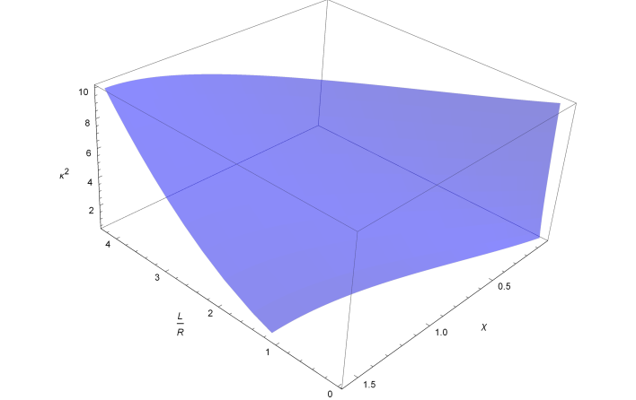
Figure 13: In the parameter space $(\chi,L/R,\chi)$ we have plotted the critical surface, namely the set of point for which the area of the connected solution is equal to the one of the dome.

4 Perturbation Theory

4.1 Perturbation theory: the non-BPS case

In order to obtain explicit results at perturbative level one should consider field configurations expanded around the supersymmetric vacuum (2.6): the determination of the effective propagators and interaction vertices in this background needs a careful and non-trivial diagonalization procedure, that has been presented in Buhl-Mortensen:2016jqo . At one-loop level the effect of the defect is entirely encoded into bulk propagators and vertices: the full Wilson loop expectation value is therefore given at this order by the tree-level and one-loop contributions

$$\left\langle{\cal W}\right\rangle=\left\langle{\cal W}\right\rangle_{\left(0\right)}+\left\langle{\cal W}\right\rangle_{\left(1\right)}$$ (4.1)

The relevant computation has been already presented in Aguilera-Damia:2016bqv : indeed, already at tree-level, they found

$$\left\langle{\cal W}\right\rangle_{\left(0\right)}=N-k+\frac{\sinh\left(\frac{\pi R\sin\chi}{L}k\right)}{\sinh\left(\frac{\pi R\sin\chi}{L}\right)},$$ (4.2)

with $N-k$ corresponding to the standard tree-level contribution for the circular Wilson loop while the second term is the interesting one for the comparison with the connected string result. The one-loop part instead is given by

$$\left\langle{\cal W}\right\rangle_{\left(1\right)}=W_{\left(1\right)}+\frac{g_{YM}^{2}\left(N-k\right)R}{4\pi L}\int_{0}^{\infty}\!\!\!\!dr~{}r\!\int_{-\pi}^{\pi}\!\!\!d\delta\displaystyle\frac{\sinh\left(\frac{\left(\pi-\delta\right)R\sin\chi}{2L}k\right)}{\sinh\left(\frac{\left(\pi-\delta\right)R\sin\chi}{2L}\right)}\left(\mathcal{I}_{1}+\sin^{2}\chi\mathcal{I}_{2}\right),$$ (4.3)

where $W_{\left(1\right)}$ contains the standard contribution for the non-broken theory with $N\to(N-k)$ and another one scaling as $k^{2}$ (the two terms were named $T_{1}$ and $T_{4}$ in Aguilera-Damia:2016bqv ). Because we want to compare the string result with the perturbative computation, we can safely discard both of them, the latter being subleading with the others in the large-N limit while the former should come from string solutions that do not end on the D5-brane, not giving $\lambda\over k^{2}$ dependent corrections. More explicitly we have Aguilera-Damia:2016bqv

$$\mathcal{I}_{1}=2\cos\frac{\delta}{2}\sin\left(\frac{2Rr}{L}\cos\frac{\delta}{2}\right)I_{\frac{k}{2}}\left(r\right)K_{\frac{k}{2}}\left(r\right),$$ (4.4)

$$\mathcal{I}_{2}=\frac{\sin\left(\frac{2Rr}{L}\cos\frac{\delta}{2}\right)}{\cos\frac{\delta}{2}}\left(\frac{k-1}{2k}I_{\frac{k+2}{2}}\left(r\right)K_{\frac{k+2}{2}}\left(r\right)+\frac{k+1}{2k}I_{\frac{k-2}{2}}\left(r\right)K_{\frac{k-2}{2}}\left(r\right)-I_{\frac{k}{2}}\left(r\right)K_{\frac{k}{2}}\left(r\right)\right).$$ (4.5)

As expected these expressions depend on $R$ and $L$ only through the ratio $\frac{R}{L}$. When $\chi\neq 0$ the integrals are very difficult to be performed analytically but, in the limit of large $k$, they can evaluated to extract their $\lambda/k^{2}$ behavior. The relevant technique has been already settled in Aguilera-Damia:2016bqv , where the focus was on the limit $L/R\to 0$. As far as $\sin\chi\neq 0$ both $\left\langle{\cal W}\right\rangle_{\left(0\right)}$ and $\left\langle{\cal W}\right\rangle_{\left(1\right)}$ exhibit an exponential behavior in $k$, that can be evaluated elementary in $\left\langle{\cal W}\right\rangle_{\left(0\right)}$ and through a saddle-point approximation in the integrals defining $\left\langle{\cal W}\right\rangle_{\left(1\right)}$. We stress that the ratio $R/L$ can be taken finite in this computation, sending just the parameter $k$ to infinity. Repeating the same same step as in Aguilera-Damia:2016bqv we end up with

$$\log\left\langle{\cal W}\right\rangle\simeq-\frac{k\pi R}{L}\left(\sin\chi+\frac{\lambda}{4\pi^{2}k^{2}}\left(\frac{\pi}{2}-\chi-\frac{1}{2}\sin 2\chi\right)\sec^{3}\chi\left(\sin^{2}\chi+\left(\frac{L}{R}\right)^{2}\right)+O\left(\frac{\lambda^{2}}{\pi^{4}k^{4}}\right)\right).$$ (4.6)

We will see in the next section that a perfect match with the strong coupling result at order $\frac{\lambda}{k^{2}}$ is obtained, without resorting to any limit on $R/L$.

4.2 Comparing perturbative analysis with the strong coupling analysis

Usually, in the AdS/CFT correspondence, perturbative computations and the supergravity analysis live in opposite regime and cannot be successfully compared. For this class of defect conformal field theories, one can instead consider a double-scaling limit Nagasaki:2011ue ; deLeeuw:2016vgp that opens a new window. Gravity computations, which are valid for large ’t Hooft coupling $\lambda$, can be considered for large $k$ in such a way that $\lambda/k^{2}$ is kept small and the results are found to be expressible in powers of $\lambda/k^{2}$. Thus, in this regime, it is possible to successfully compare gauge and gravity results providing further non-trivial verifications of the AdS/CFT correspondence.

In the strong coupling regime, this limit is equivalent to expand our classical solution in power of $\frac{1}{\kappa^{2}}$, namely for large value of the flux. The flux diverges when the denominator in eq. (2.38) vanishes, but the numerator does not. This occurs when $x$, $m$ and $\chi$ satisfy the relation

$$m~{}x^{2}~{}\text{cn}\left(\left.\frac{1}{2}x(\pi-2\chi)\right|m\right)^{2}+x^{2}-1=0.$$ (4.7)

Even though we are considering the regime in which $\kappa^{2}$ is very large and eventually diverges, we require that the (adimensional) distance $L/R$ of the Wilson loop from the defect remains finite. The parameter $\eta=\text{arcsinh}\frac{L}{R}$ in terms of $x$, $m$ and $\chi$ is the sum of two positive contributions. In fact, in eq. (2.37) the first term is the integral of a positive function, while the second one is the $\tanh^{-1}$ of a positive argument. If use the eq. (2.38) we can recast the argument of $\tanh^{-1}$ in the following form:

$$\sqrt{\frac{2\kappa^{2}\left(1-(m+1)x^{2}\right)}{\kappa^{2}\left(1-(m+1)x^{2}\right)-(m+1)x^{2}+\sqrt{\left(\kappa^{2}\left(1-(m+1)x^{2}\right)-(m+1)x^{2}\right)^{2}-4\left(\kappa^{2}+1\right)mx^{4}}+2}},$$ (4.8)

which allows us to study easily its behavior for large $\kappa^{2}$. If the $m$ and $x$ are finite when $\kappa^{2}\to\infty$ and the combination $1-(m+1)x^{2}$ does not vanish, it is straightforward to realize that the quantity in eq. (4.8) approaches $1$. Therefore its contribution to the distance ($\tanh^{-1}(1)$) diverges. To avoid this conclusion we must require

$$x=\frac{1}{\sqrt{1+m}}+O\left(\frac{1}{\kappa^{2}}\right)\ \ \ \ \ \ \ \kappa\to\infty.$$ (4.9)

If we use the definition of the unknown $x$, the above result is equivalent to require that $j^{2}=O(\kappa^{2})$, therefore we are in the region (A). In this limit, with the help of the expansion eq. (4.9), eq. (4.7) collapses to

$$\frac{m}{m+1}~{}\text{sn}\left(\left.\frac{1}{2\sqrt{1+m}}x(\pi-2\chi)\right|m\right)^{2}=0\ \ \ \Rightarrow\ \ \ \ m=0.$$ (4.10)

The requirement that the distance is kept finite and different from zero fixes as $m$ must vanish for large $\kappa$: $m=O\left(\frac{1}{\kappa^{2}}\right)$. Therefore, in this regime we can safely assume the following expansion for the parameters:

$$m=\sum_{n=1}^{\infty}\frac{a_{2n}}{\kappa^{2n}}\ \ \ \ \ \ \ \ \ \ \ \ \ \ \ \ \ \ \ \ \ x=1+\sum_{n=1}^{\infty}\frac{b_{2n}}{\kappa^{2n}}$$ (4.11)

The coefficients can be determined by solving iteratively the equation for the flux and the condition fixing the distance (see app. C). At the lowest order we get

$$m= \frac{\sec^{2}\chi}{\kappa^{2}}\left(1-\left(\frac{L^{2}}{R^{2}}+1\right)\sec^{2}\chi\right)+O\left(\frac{1}{\kappa^{4}}\right)$$ (4.12a)

$$x= 1+\frac{1}{2\kappa^{2}}\left(\frac{L^{2}}{R^{2}}+1\right)\tan^{2}\chi\sec^{2}\chi+O\left(\frac{1}{\kappa^{4}}\right)$$ (4.12b)

The subsequent terms in the expansion are quite cumbersome and their explicit form up to $$1/\kappa^{4}$$ is given in app. C.

We can now use this expansion (see app. C) to determine the first two terms in the large $\kappa$ expansion

$$\begin{split}{S}=&-\frac{\sqrt{\lambda}\kappa R}{L}\left[\sin\chi+\frac{1}{4\kappa^{2}}{\left(\frac{\pi}{2}-\chi-\frac{1}{2}\sin 2\chi\right)\sec^{3}\chi\left(\sin^{2}\chi+\frac{L^{2}}{R^{2}}\right)}\right]+O\left({\kappa}^{-2}\right)=\\ =&-\frac{\pi kR}{L}\left[\sin\chi+\frac{\lambda}{4\pi^{2}k^{2}}{\left(\frac{\pi}{2}-\chi-\frac{1}{2}\sin 2\chi\right)\sec^{3}\chi\left(\sin^{2}\chi+\frac{L^{2}}{R^{2}}\right)}+O\left(\frac{\lambda^{2}}{\pi^{4}k^{4}}\right)\right],\end{split}$$ (4.13)

where we have replaced the strong coupling quantity $\kappa$ with its expression in terms of $\sqrt{\lambda}$ and the integer flux $k$. A simple power-counting of the coupling constant immediately shows that this are only two terms which can be compared with our perturbative computation and they successfully reproduce eq. (4.6).

4.3 Perturbation theory: the BPS case

We have already seen that at $\chi=0$, when the Wilson loop only couples to the massless scalar $\Phi_{6}$ and we are therefore at the BPS point, the connected string solution does not exist. At weak coupling we expect conversely that the scaling $\lambda/k^{2}$ should break: let us examine more closely the situation. We start by observing that a dramatic simplification occurs at the perturbative level, the non-trivial contribution at one-loop reducing to a much simpler expression

$$\left\langle{\cal W}\right\rangle_{\left(1\right)}=W_{\left(1\right)}+\frac{g_{YM}^{2}\left(N-k\right)Rk}{4\pi L}\int_{0}^{\infty}\!\!\!\!dr~{}r\!\int_{-\pi}^{\pi}d\delta~{}~{}2\cos\frac{\delta}{2}\sin\left(\frac{2Rr}{L}\cos\frac{\delta}{2}\right)I_{\frac{k}{2}}\left(r\right)K_{\frac{k}{2}}\left(r\right)\,.$$ (4.14)

The integral over the angular variable $\delta$ can be exactly performed in terms of the Bessel function $J_{1}$ leading to

$$\left\langle{\cal W}\right\rangle_{\left(1\right)}=W_{\left(1\right)}+\frac{g_{YM}^{2}\left(N-k\right)Rk}{L}\int_{0}^{\infty}\!\!\!\!dr\,r\,J_{1}\left(\frac{2Rr}{L}\right)I_{\frac{k}{2}}\left(r\right)K_{\frac{k}{2}}\left(r\right)\,,$$ (4.15)

and the radial integral is solved in terms of Meijer G Functions:

$$\begin{split}\left\langle{\cal W}\right\rangle_{\left(1\right)}&=W_{\left(1\right)}+\frac{g_{YM}^{2}\left(N-k\right)kL}{4\sqrt{\pi}R}\,G_{3,3}^{2,2}\left(\frac{R^{2}}{L^{2}}\Biggl{|}\begin{array}[]{c}1,1-\frac{k}{2},\frac{k+2}{2}\\ \frac{1}{2},\frac{3}{2},\frac{1}{2}\\ \end{array}\right)\,.\end{split}$$ (4.16)

We shall explore two interesting limits of this exact result. First we investigate the behavior of $\left\langle{\cal W}\right\rangle_{\left(1\right)}$ when the parameter $k$ goes to $\infty$. This limit is easier to discuss if we step back to the integral form of the one-loop expression and perform the change of variables $r\to\frac{k}{2}r$

$$\left\langle{\cal W}\right\rangle_{\left(1\right)}=W_{\left(1\right)}+\frac{g_{YM}^{2}\left(N-k\right)R}{4L}k^{3}\int_{0}^{\infty}\!\!\!\!dr\,r\,J_{1}\left(\frac{Rkr}{L}\right)I_{\frac{k}{2}}\left(\frac{kr}{2}\right)K_{\frac{k}{2}}\left(\frac{kr}{2}\right).$$ (4.17)

Then we can use the following asymptotic expansions for the product of the modified Bessel functions

$$K_{\frac{k}{2}}\left(\frac{kr}{2}\right)I_{\frac{k}{2}}\left(\frac{kr}{2}\right)=\frac{1}{k(1+r^{2})^{1/2}}\sum_{n=0}^{\infty}\frac{2^{2n}}{k^{2n}}\sum^{2n}_{m=0}(-1)^{m}U_{2n-m}((1+r^{2})^{-\frac{1}{2}})U_{m}((1+r^{2})^{-\frac{1}{2}}),$$ (4.18)

which is obtained by combining the expansion 10.41.3 and 10.41.4 of Nist . The $U_{n}(x)$ are polynomials that can be constructed recursively (see sec. 10.41 in Nist for details): $U_{0}(x)=1,U_{1}(x)=\frac{x}{8}-\frac{5x^{3}}{24},\dots$. If we are interested at the leading order in $k$, it is sufficient to consider the first term in the expansion:

$$\begin{split}\left\langle{\cal W}\right\rangle_{\left(1\right)}&\simeq W_{\left(1\right)}+\frac{g_{YM}^{2}\left(N-k\right)R}{4L}k^{2}\int_{0}^{\infty}\!\!\!\!drJ_{1}\left(\frac{Rkr}{L}\right)\frac{r}{(1+r^{2})^{1/2}}=\\ =&W_{\left(1\right)}+\frac{g_{YM}^{2}\left(N-k\right)L}{4R}\frac{2}{\sqrt{\pi}}G_{1,3}^{2,1}\left(\frac{k^{2}R^{2}}{4L^{2}}\Biggl{|}\begin{array}[]{c}1\\ \frac{1}{2},\frac{3}{2},\frac{1}{2}\\ \end{array}\right)=\\ =&W_{\left(1\right)}+\lambda\frac{L}{4R}\left(1+O\left(\frac{1}{k^{2}}\right)\right).\end{split}$$ (4.19)

The BPS circle does not possess the correct scaling to match a potential connected string solution: its expansion does not organize in a $\lambda/k^{2}$ series. This corroborates the absence of a connected solution the BPS case.
The second limit we shall consider is $R\to 0$, namely when we shrink the loop to a point. Since we are dealing with a conformal field theory, it is the dimensionless combination $x=R/L$, which approaches to zero: this should also correspond to place the Wilson loop at infinite distance from the defect, recovering at leading order the expectation value of the usual BPS circle. We find

$$\begin{split}\left\langle{\cal W}\right\rangle_{\left(1\right)}&=W_{\left(1\right)}\!+\!\frac{g_{YM}^{2}k(N-k)}{4}\left[1\!-\!\frac{1}{4}\left(1\!-\!k^{2}\right)x^{2}\left(\psi\left(\frac{k+1}{2}\right)\!+\!\gamma_{E}+\log x\!-\!\log 2\right)\!-\!\right.\\ &\hskip 142.26378pt-\left.\frac{x^{2}}{2}+O\left(x^{4}\right)\right].\end{split}$$ (4.20)

As expected we see that the leading term scales as a constant in this limit, and when combined with $W_{(1)}$ it reconstructs at this order the circular Wilson loop in absence of defect. Actually the next term in the expansion can be easily understood in terms of the operator product expansion (OPE) of the circular BPS loop.

4.4 Operator product expansion expansion of the Wilson loop

In absence of defect the Wilson loop, when probed from a distance much larger than the size of the loop itself, can approximated in CFT by an expansion of local operators Berenstein:1998ij ; Arutyunov:2001hs

$$\frac{\mathcal{W}(\mathcal{C})}{\left\langle\mathcal{W}(\mathcal{C})\right\rangle}=\mathds{1}+\sum_{k}c_{k}R^{\Delta_{k}}\,\mathcal{O}^{(k)}(x)\,,$$ (4.21)

where $R$ is the radius of the loop, the $\mathcal{O}^{(k)}$ are composite operators with conformal weights $\Delta_{k}$ evaluated at the center of the loop, and $c_{k}$ are the OPE coefficients that depend on $\lambda$. In perturbation theory the scaling dimension of an operator can be represented as

$$\Delta=\Delta^{(0)}+\Delta^{(1)}+\Delta^{(2)}+\cdots\,,$$ (4.22)

where $\Delta^{(0)}$ is the free field dimension, and $\Delta^{(1)},\Delta^{(2)}$ are anomalous dimensions at order $\lambda$, $\lambda^{2}$ and so on. Since the symmetries of a CFT constraint the one-point functions of operators that are not the identity to be zero in absence of defects, the expectation value of the Wilson loop corresponds to the coefficient of the identity. The OPE coefficients can be computed perturbatively, but the result cannot be extrapolated in general to strong coupling. The operators appearing in eq. (4.21) must have the same properties as the Wilson loop, the $\mathcal{O}^{(k)}$ being therefore bosonic and gauge invariant. The possible contributions to the OPE for low value of the scaling dimension are

• $\Delta^{(0)}=0:$ the only possible contribution comes from operators proportional to the identity;

• $\Delta^{(0)}=1:$ the only elementary fields with scaling dimension one are the scalars. The trace of a single scalar is the only gauge-invariant operator, but since the $\Phi_{I}$’s are valued in the Lie algebra $\mathfrak{su}(N)$ this contribution vanishes;

• $\Delta^{(0)}=2:$ the only two types of gauge-invariant operators are the chiral primary operators $\mathcal{O}^{a}$ and the Konishi scalar $\mathcal{K}$. They are canonically normalized as

  $$\mathcal{O}^{a}=4\sqrt{2}\pi^{2}C^{a}_{IJ}\,\text{:}\text{Tr}(\Phi^{I}\Phi^{J}):\,,\qquad\mathcal{K}=\frac{4\pi^{2}}{\sqrt{3}}:\text{Tr}(\Phi^{I}\Phi^{I}):.$$ (4.23)

  Here the traceless symmetric tensor $C^{a}_{IJ}$ obeys $C^{a}_{IJ}C^{b}_{IJ}=\delta^{ab}$ with $a,b=1,\dots,20.$ The operators $\mathcal{O}^{a}$ lie in a short supermultiplet and transform in the $\mathbf{20}$ irreducible representation of the R-symmetry group $SO(6)_{R}$. They have vanishing anomalous dimension. The Konishi scalar is the lowest component of the long supermultiplet Konishi:1983hf , and it acquires an anomalous dimension in perturbation theory. Its one-loop anomalous dimension is $\Delta^{(1)}=\frac{3\lambda}{4\pi^{2}}$ Anselmi:1998ms ; Bianchi:1999ge ; Arutyunov:2000ku ; Arutyunov:2000im ; Arutyunov:2001mh ; Penati:2001sv .

Given the expansion eq. (4.22) for the scaling dimension, every term $R^{\Delta}$ in eq. (4.21) produces logarithmic terms as

$$R^{\Delta}=R^{\Delta^{(0)}}\left(1+\Delta^{(1)}\log R+\Delta^{(2)}\log R+\frac{1}{2}\Delta^{(1)^{2}}\log^{2}R+\cdots\right)\,,$$ (4.24)

in the limit $R\rightarrow 0$ the coefficients of the divergent logarithms $\log R$ is proportional to the one-loop anomalous dimensions of the non-protected operators appearing in the Wilson loop OPE, as the Konishi operator. The OPE coefficients can be read off from the correlation functions of the Wilson loop with local operators: in particular one can consider CPOs with scaling dimension $\Delta\equiv k$ defined as

$$\mathcal{O}_{k}^{I}(x)=\frac{(8\pi^{2})^{k/2}}{\sqrt{k}}C^{I}_{J_{1}\cdots J_{k}}:\text{Tr}(\Phi^{J_{1}}\cdots\Phi^{J_{k}}):\,,$$ (4.25)

where $C^{I}_{J_{1}\cdots J_{k}}$ are totally symmetric traceless tensors normalized as $C^{I}_{J_{1}\dots J_{k}}C^{L}_{J_{1}\dots J_{k}}=\delta^{IL}$. If $k=2$, one obtains the chiral primary operator $\mathcal{O}^{a}$ with $\Delta=2$. It is possible to show that their two-point functions are protected by supersymmetry and their scaling dimensions do not receive radiative corrections. From the exact expression for correlators of the circular Wilson loop with CPOs eq. (4.25) valid for any $\lambda$ found in Semenoff:2001xp it is possible to recover the relevant OPE coefficients at any order

$$c^{I}_{k}=\frac{2^{k/2-1}}{N}\sqrt{\frac{k}{\lambda}}\,\frac{I_{k}(\sqrt{\lambda})}{I_{1}(\sqrt{\lambda})}Y^{I}(\theta),$$ (4.26)

where $I_{k}$ and $I_{1}$ are modified Bessel functions and $Y^{I}(\theta)$ are spherical harmonics

$$Y^{I}(\theta)=C_{J_{1}\dots J_{k}}^{I}\theta^{J_{1}}\cdots\theta^{J_{k}}$$ (4.27)

with the index $I$ running over all the spherical harmonics of $SO(6)$ Casimir Lee:1998bxa . Perturbatively, the leading contribution to the correlation functions of the circular Wilson loop with the chiral primary with smallest conformal dimension and the Konishi operator was found in Arutyunov:2001hs giving

$$c^{a}_{\mathcal{O}}=\frac{1}{2\sqrt{2}N}Y^{a}(\theta)\,,\qquad c_{1}=\frac{1}{4\sqrt{3}N}.$$ (4.28)

Summarizing the lower dimensional content of the local operator expansion, we have

$$\begin{split}\frac{\mathcal{W}(\mathcal{C})}{\left\langle\mathcal{W}(\mathcal{C})\right\rangle}=&\mathds{1}+R^{\Delta_{\mathcal{K}}}\left(\frac{1}{4\sqrt{3}N}+\frac{\lambda c_{2}}{N}+\cdots\right)\mathcal{K}(x)+\\ &+R^{\Delta_{\mathcal{O}}}\left(\frac{1}{2\sqrt{2}N}-\frac{\lambda}{48\sqrt{2}N}+\cdots\right)Y_{a}(\theta)\mathcal{O}^{a}(x)+\text{higher scaling dimension}\,,\end{split}$$ (4.29)

the dots indicate higher order terms in $\lambda$ of the corresponding operator expansion coefficients. The value of $c_{2}$ for the Konishi operator has not been computed, at least at our knowledge, while the OPE coefficient at order $\lambda$ for the chiral primary operator with $k=2$ is obtained expanding for small $\lambda$ the r.h.s of eq. (4.26). The scaling dimension of $\mathcal{O}^{a}$ is $\Delta_{\mathcal{O}}=2$ and this operator does not get an anomalous dimension, whereas $\Delta_{\mathcal{K}}$ receives perturbative corrections and following eq. (4.24) one can write

$$R^{\Delta_{\mathcal{K}}}=R^{2}\left(1+\Delta_{\mathcal{K}}^{(1)}\log R+\cdots\right)\,.$$ (4.30)

4.5 Wilson loop OPE and one-point functions

In the presence of a defect we expect that the structure of the OPE for the circular Wilson loop is unchanged, due to the fact that we are effectively probing the operator at infinite distance or, alternatively, because the ultraviolet properties of the theory are insensible to the boundary. The only modification needed is implied by the presence of non-trivial one-point functions: the Wilson coefficient of the identity is unchanged and takes into account still the contribution of the expectation value ${\langle\mathcal{W}\rangle_{0}}$ in absence of defect. We are led therefore to assume the following OPE in the defect theory

$$\begin{split}\frac{\mathcal{W}}{\langle\mathcal{W}\rangle_{0}}=&\mathds{1}+R^{\Delta_{\mathcal{K}}}\left(\frac{1}{4\sqrt{3}N}+\frac{\lambda c_{2}}{N}+\cdots\right)\mathcal{K}(x)+\\ &+R^{2}\left(\frac{1}{2\sqrt{2}N}-\frac{\lambda}{48\sqrt{2}N}+\cdots\right)Y_{a}(\theta)\mathcal{O}^{a}(x)+\text{higher scaling dimension}\,,\end{split}$$ (4.31)

the expansion being normalized using $\langle\mathcal{W}\rangle_{0}$. For the explicit definition of $C^{a}_{ij}$ and $Y^{a}$ see Appendix F. Now taking the vacuum expectation value of eq. (4.31) we understand that the expansion we have derived for the Wilson loop for $R/L\to 0$ (see eq. (4.20)) should be recovered from the one-point functions of the Konishi operator $\mathcal{K}(x)$ and of the combination of chiral primaries $Y_{a}(\theta)\mathcal{O}^{a}(x)$, from the one-loop anomalous dimension of $\mathcal{K}(x)$ and from the Wilson coefficient $c_{2}$. Fortunately in a beautiful series of papers deLeeuw:2015hxa ; Buhl-Mortensen:2015gfd ; Buhl-Mortensen:2017ind the NBI group has studied the one-point functions of scalar operators in the defect theory, obtaining explicit result both at tree and one-loop level through perturbative computations and at all-order applying integrability techniques. We take advantage of their efforts and we adapt their results to our relevant operators (see Appendix F for the full details)

$$\langle Y_{a}(\theta)\mathcal{O}^{a}(x)\rangle=\frac{\pi^{2}}{3\sqrt{2}L^{2}}k(1-k^{2})-\frac{\lambda}{2\sqrt{2}NL^{2}}\left(k(N-k)+\frac{k^{2}-1}{2}\right)$$ (4.32)

$$\langle\mathcal{K}(x)\rangle=-\frac{\pi^{2}}{\sqrt{3}L^{2}}k(1-k^{2})-\frac{\sqrt{3}\lambda}{4L^{2}}k\left(1-k^{2}\right)\left(\psi\left(\frac{k+1}{2}\right)+\gamma_{E}-\log 2+\frac{5}{6}\right).$$ (4.33)

Using further the one-loop contribution to the anomalous dimension of the Konishi operator $\Delta^{(1)}=\frac{3\lambda}{4\pi^{2}}$ we can compare the OPE expansion with the direct computation of the Wilson loop in the small $R/L$ limit eq. (4.20). We see that our result non-trivially matches with the one-point functions derived in deLeeuw:2015hxa ; Buhl-Mortensen:2015gfd ; Buhl-Mortensen:2017ind if

$$c_{2}=-\frac{15+\pi^{2}}{96\sqrt{3}\pi^{2}}$$ (4.34)

Thus, from the OPE for the Wilson loop in the defect case, we have a prediction for the Wilson coefficient of the Konishi operator at order $\lambda$ in eq. (4.29). This prediction could be verified by computing the two-loop contribution to the two-point function of the Konishi operator with the circular Wilson loop in absence of defect.

5 Conclusions and outlook

The introduction of defects in conformal field theories implies, in general, an augment of the independent conformal data and enriches the dynamics with novel effects that certainly deserve further studies. While at level of correlation functions of local operators there has been a considerable amount of investigations in this field, much less attention has been devoted to the behavior of non-local operator: in this paper we tried to fill partially this gap, studying the fate of the circular Wilson loop in the defect ${\cal N}=4$ Super Yang-Mills theory both at strong and weak coupling. In the former case, using AdS/CFT correspondence, we have explored in full generality the structure of the vacuum expectation value of a loop parallel to the defect, finding the semiclassical string solution in the complete parameter space and computing the related classical action. The main result has been the discovery of a novel Gross-Ooguri type transition, separating a phase in which the dome solution, associated with the Wilson loop in absence of defect, dominates from a situation in which a cylindrical minimal surface attached to the defect D5 brane describes the non-local operator. In the generic case, we have performed a double-scaling limit on our cylindrical solution, sending $k\to\infty$ with $\lambda/k^{2}$ fixed, recovering without resorting to any geometrical approximation the perturbative Feynman diagram result. For the particular case in which the Wilson loop operator becomes BPS, $i.e.$ for $\chi=0$ in our notation, the connected solution ceases to exist and the strong coupling regime is arguably described by supergravity exchanges between the spherical dome and the D5 brane. Conversely, we found an analogous behavior at weak coupling, the BPS case not respecting the expected double-scaling limit. For the BPS case we have also explored at one-loop the shrinking (or equivalently the large distance) behavior, finding that it can be nicely understood in terms of the OPE of the Wilson loop operator: the knowledge of the non-trivial one-point functions for scalar operators of classical dimension two allows to reconstruct explicitly the first terms of the expansion. Assuming a certain value for the one-loop contribution to the relevant Wilson coefficient of the Konishi operator we find a perfect matching between our computations and the results of deLeeuw:2015hxa ; Buhl-Mortensen:2015gfd ; Buhl-Mortensen:2017ind .

There are a number of different directions that can be explored in order to improve the present investigations. First of all one should compute independently the Wilson coefficient for the Konishi in the circular BPS Wilson loop OPE: this would represent a non-trivial check of the result obtained for one-point functions in deLeeuw:2015hxa ; Buhl-Mortensen:2015gfd ; Buhl-Mortensen:2017ind or would enlighten potential subtleties in our OPE description. A second and intriguing question concerns the short-distance limit from the defect (or equivalently the large radius limit of the loop) in the BPS case. Let us consider the expansion of eq. (4.19) in the limit $L\to 0$ namely $x\to\infty$: for odd values of $k$ we find an analytical series in inverse odd powers of $x$:

$$\left\langle{\cal W}\right\rangle_{\left(1\right)}=W_{\left(1\right)}+\frac{g_{YM}^{2}\left(N-k\right)}{4}\left[\frac{1}{x}-\frac{3}{\left(8-2k^{2}\right)x^{3}}+O\left(\left(\frac{1}{x}\right)^{4}\right)\right].$$ (5.1)

For even $k$ instead we observe the appearance also of logarithmic corrections that start at the order $x^{-k-1}$. For instance for $k=4$ we find

$$W_{\left(1\right)}+g_{YM}^{2}\left(N-4\right)\left[\frac{1}{4x}+\frac{1}{32x^{3}}+\frac{3(120\log(8x)-289)}{8192x^{5}}-\frac{25(168\log(8x)-367)}{65536x^{7}}+O\left(\frac{1}{x^{8}}\right)\right].$$ (5.2)

It would be tempting to interpret these expressions in terms of a boundary operator expansion (BOE) of the Wilson loop: BOE in defect ${\cal N}=4$ SYM has been already considered for scalar two-point functions in deLeeuw:2017dkd . In this paper the spectrum of gauge-invariant boundary operators of the theory has been also presented (see also Ipsen:2019jne ): it would be interesting to derive a version of the BOE for the circular BPS Wilson loop and to use the consistency of bulk and boundary operator expansions to get new information on the defect theory. A puzzling aspect of the above computations is that their analytical properties depend crucially on $k$. For odd $k$ the absence of logarithm suggests that only protected operators should appear in the BOE, while for even $k$ also non-protected operators seem to be part of the game.

In the BPS case we have found an exact analytical expression for the vacuum expectation value of the Wilson loop at the first perturbative order and we have observed that no connected string solution appears at strong coupling: these two facts might signal that an exact evaluation of this Wilson loop could be feasible, resorting probably to a highly non-trivial application of supersymmetric localization in this context.

A more direct and conceptually straightforward follow-up of our investigations concerns the case of the correlator of two circular Wilson loop in the defect set-up avvenire : the case of two straight-line has been already tackled in Preti:2017fhw where a complicate pattern of Gross-Ooguri like phase transition has been discovered for the quark-antiquark potential. In the circular case, the situation is more complicated because of the larger parameter space and the possibility to have both ”undefected” connected string solutions between the two circles or individual cylinder/dome solutions dominating the semiclassical strong coupling regime. Non-trivial string three-point functions could also enter the game, describing new connected minimal surfaces with three holes, one of which lying on the D5 brane.

Finally, the generalization of our investigation in the cousin theories related to the non-supersymmetric D3/D7 system could be certainly considered.

Acknowledgements

Special thanks go to Marisa Bonini for participating at the early stages of this work and many interesting discussions. It is also our pleasure to thank L. Bianchi, A. Bissi, N. Drukker, C. Kristjansen, S. Penati, M. Preti, D. Trancanelli, E. Vescovi and K. Zarembo for useful discussions.

Appendix A Expression for the distance from the defect

The distance eq. (2.37) from the defect brane can be also expressed in terms of the elliptic integral of the third kind if we explicitly perform the integration defining the auxiliary function $v(\sigma)$. We obtain

$$\eta= \sqrt{-\frac{(j^{2}m+1)(j^{2}+m)}{(m+1)(j^{2}-1)}}\left[\sqrt{\frac{j^{2}-1}{m+1}}\tilde{\sigma}-\Pi\left(-\frac{m+1}{j^{2}-1};\left.\text{am}\left(\left.\sqrt{\frac{j^{2}-1}{m+1}}\tilde{\sigma}\right|m\right)\right|m\right)\right]+\noindent$$

$$\ \ \ \ \ \ \ \ \ \ \ \ \ \ +\tanh^{-1}\!\!\left(-\sqrt{-\frac{(m+1)^{2}}{(j^{2}m+1)(j^{2}+m)}}\frac{g^{\prime}(\tilde{\sigma})}{g(\tilde{\sigma})}\right)=$$ (A.1)

$$= \sqrt{-\frac{(n+1)(nm+1)}{n}}\left[\sqrt{n}\tilde{\sigma}-\Pi\left(\left.-\frac{1}{n};\text{am}(\sqrt{n}\tilde{\sigma}|m)\right|m\right)\right]\!+\!\tanh^{-1}\!\!\left(\frac{-\frac{g^{\prime}(\tilde{\sigma})}{g(\tilde{\sigma})}}{\sqrt{-(nm+1)(n+1)}}\right)$$

where we have introduced the short-hand notation

$$n\equiv\frac{j^{2}-1}{m+1}.$$ (A.2)

This second representation of the distance will be useful when doing analytical expansions, the one provided by eq. (2.37) being more suitable in numerical analysis.

For instance, from eq. (A) is quite straightforward to see that the distance vanishes when $m$ approaches $m_{c}$. We first observe that the argument of the arctanh behaves like

$$\sim\frac{\sqrt{n}}{n\sqrt{-m_{c}}}\frac{\text{cn}(\sqrt{n}\tilde{\sigma}|m)\text{dn}(\sqrt{n}\tilde{\sigma}|m)}{\text{sn}(\sqrt{n}\tilde{\sigma}|m)}=\frac{s_{0}}{\sqrt{n}},$$ (A.3)

where we have taken into account that the combination $\sqrt{n}\tilde{\sigma}$ is finite in this limit: it vanishes since $n\to\infty$ as $m\to m_{c}$ (see eq. (3.4)).The remaining contribution can be also seen to vanish when we exploit the behavior of the incomplete elliptic integral of the third kind for small values of its first argument. In fact we have wolfram

$$\Pi\left(\left.-\frac{1}{n};\text{am}(\sqrt{n}\tilde{\sigma}|m)\right|m\right)\simeq z+{c(z,m)}\frac{1}{n}+O\left(\frac{1}{n^{2}}\right),$$ (A.4)

which in turn implies that this contribution also vanishes as $1/\sqrt{n}$.

Appendix B Expansion of $n$, $g(\tilde{\sigma})$ and $\frac{\partial\eta}{\partial m}$ close to the boundary $j^{2}=-1/m^{2}$

In the parameter space the boundary $j^{2}=-1/m^{2}$ corresponds to the curved red line plotted in fig. 2. The values of $\chi$ and $m$ along this curve are related by eq. (3.5). Our goal is now to expand some relevant quantities in the region close to this boundary. To begin with, we shall choose a value for the angle: $\chi=\chi_{0}$. Eq. (3.5) allows us to translate it in a value $m_{0}$ for $m$. Given the pair $(\chi_{0},m_{0})$ on the red curve, the value $x$ is fixed by eq. (2.49) to be

$$x_{0}=1.$$ (B.1)

We now expand around this configuration. Specifically we keep the angle $\chi_{0}$ fixed and we allow $m$ to be different from $m_{0}$, but close to it. Then we can write $x$ as series expansion around $m_{0}$:

$$x=1+s_{1}(m-m_{0})+s_{2}(m-m_{0})^{2}+O((m-m_{0})^{3}).$$ (B.2)

The coefficients $s_{i}$ can be determined by solving perturbatively eq. (2.38). With help of Mathematica and after some trivial manipulations one finds

$$x=1+\frac{\left(m-m_{0}\right){}^{2}\left(\kappa^{2}m_{0}+m_{0}-1\right)\left(\left(m_{0}-1\right)\mathds{K}\left(m_{0}\right)+\mathds{E}\left(m_{0}\right)\right){}^{2}}{8\kappa^{2}\left(m_{0}-1\right)m_{0}^{2}}+O\left(\left(m-m_{0}\right){}^{3}\right).$$ (B.3)

Given eq. (B.3) the corresponding expansion for $n$ around $m=m_{0}$ is easily recovered

$$\begin{split}n=\frac{x^{2}}{1-(m+1)x^{2}}=-\frac{1}{m_{0}}+\frac{m-m_{0}}{m_{0}^{2}}-\frac{a_{0}}{m_{0}^{3}}(m-m_{0})^{2}+O((m-m_{0})^{3})\\ \ \ \textrm{with}\quad\quad a_{0}=1-\frac{\left(\kappa^{2}m_{0}+m_{0}-1\right)\left(\left(m_{0}-1\right)\mathds{K}\left(m_{0}\right)+\mathds{E}\left(m_{0}\right)\right){}^{2}}{4\kappa^{2}\left(m_{0}-1\right)m_{0}}.\end{split}$$ (B.4)

Next we can use eqs. (B.3) and (B.4) to evaluate the expansion of $g(\tilde{\sigma})$ and $g^{\prime}(\tilde{\sigma})$, two quantities that often appears in our analysis. The simplest way to calculate $g(\tilde{\sigma})$ is to use eq. (2.26) and eq. (2.38) to obtain an expression as a function of $n,m,x$ and $\kappa$. We find

$$g(\tilde{\sigma})= \sqrt{-\frac{2\left(\kappa^{2}+1\right)mnx^{2}}{\kappa^{2}+\left(\kappa^{2}+1\right)(-(m+1))x^{2}+\sqrt{\left(\kappa^{2}-\left(\kappa^{2}+1\right)(m+1)x^{2}\right)^{2}-4\left(\kappa^{2}+1\right)mx^{4}}}}=$$

$$= \frac{1}{\sqrt{-m_{0}}}+\frac{m-m_{0}}{2\left(-m_{0}\right){}^{3/2}}+$$

$$+\frac{(4a_{0}-1)\left(m_{0}-1\right)-\left(\left(m_{0}-1\right)\mathds{K}\left(m_{0}\right)+\mathds{E}\left(m_{0}\right)\right){}^{2}}{8\left(m_{0}-1\right)\left(-m_{0}\right){}^{5/2}}\left(m-m_{0}\right){}^{2}+O\left(\left(m-m_{0}\right){}^{3}\right).$$ (B.5)

Similarly for $g^{\prime}(\tilde{\sigma})$ we have

$$g^{\prime}(\tilde{\sigma})= -\kappa\sqrt{-mn^{2}-g^{2}(\tilde{\sigma})}=\frac{\left(m-m_{0}\right)\left(\left(m_{0}-1\right)\mathds{K}\left(m_{0}\right)+\mathds{E}\left(m_{0}\right)\right)}{2m_{0}^{2}}+O\left(\left(m-m_{0}\right){}^{2}\right).$$ (B.6)

If we now plug these results into eq. (3.1) for the derivative of $\eta$, we get at $m=m_{0}$:

$$\begin{split}\left.\frac{\partial\eta}{\partial m}\right|_{m=m_{0}}=&\frac{\left(1-m_{0}\right)\left(\mathds{E}\left(m_{0}\right)+(m_{0}-1)\mathds{K}\left(m_{0}\right)\right){}^{2}+m_{0}\kappa^{2}\left(1-\left(\mathds{E}\left(m_{0}\right)+\left(m_{0}-1\right)\mathds{K}\left(m_{0}\right)\right){}^{2}\right)}{2\kappa\left(1-m_{0}\right)\left(-m_{0}\right){}^{3/2}\sqrt{1-\left(\kappa^{2}+1\right)m_{0}}}.\end{split}$$ (B.7)

This value of the derivative has been instrumental in sec. 3.1 to investigate the monotonicity of $\eta$ with $m$.

Appendix C The Expansion of then renormalized area for $\kappa\to\infty$

Our goal, here, is to expand the renormalized area for $\kappa\to\infty$ while keeping constant the distance $L$ from the defect. From the numerical analysis in sec. 3.1, we see that the same value of $L$ is reached for smaller and smaller value of $m$ as $\kappa$ approaches infinity (at least if $\chi\neq\frac{\pi}{2}$). Thus we shall assume

$$m\to 0\ \ \ \ \ \ \ \mbox{when}\ \ \ \kappa\to\infty\ \ \ \mbox{but $L$ is fixed.}$$ (C.1)

In this limit we can easily check that $x\to 1$ by solving eq. (2.38). We are motivated therefore to postulate the following expansion of $m$ and $x$ for large flux

$$m=\sum_{n=1}^{\infty}\frac{a_{2n}}{\kappa^{2n}}\ \ \ \ \ \ \ \ x=1+\sum_{n=1}^{\infty}\frac{b_{2n}}{\kappa^{2n}}.$$ (C.2)

At this level it is just an ansatz that will be justified by its consistency. Expanding in this way eq. (2.38) and eq. (A) is potentially a delicate issue since all the entries of the elliptic functions depend explicitly or implicitly on the modulus $m$: the results below are obtained by first computing the elliptic function for small modulus keeping the other entries fixed and subsequently expanding the dependence on the other entries for small $m$.

With this procedure eq. (2.38) determining the flux reads

$$\kappa^{2}= \frac{\kappa^{2}}{a_{2}\cos^{2}\chi+2b_{2}\cot^{2}\chi}+\frac{1}{8\left(a_{2}\sin^{2}\chi+2b_{2}\right){}^{2}}\left[\tan\chi\left(-4\tan\chi\left(a_{4}\sin^{2}\chi+2b_{4}\right)+\right.\right.$$

$$+2a_{2}b_{2}\sec^{2}\chi\left((\pi-2\chi)\left(\sin^{2}2\chi+2\cos 2\chi\right)-4\sin 2\chi-\sin 4\chi\right)-a_{2}^{2}\sin\chi\tan^{2}\chi~{}\times$$ (C.3)

$$\left.\left.\times(4\chi\sin\chi-2\pi\sin\chi+7\cos\chi+\cos 3\chi)+4b_{2}^{2}(8\chi+3\sin 2\chi-4\pi)\sec^{2}\chi\right)\right]+O\left(\kappa^{-2}\right)\$$

and similarly eq. (A), which instead fixes the distance, takes the form

$$\frac{L}{R}= \tanh^{-1}\left(\frac{\sqrt{-\frac{\left(a_{2}+2b_{2}\right)\tan^{2}\chi}{b_{2}}}}{\sqrt{2}}\right)+\frac{1}{2\sqrt{2}\kappa^{2}}\Biggl{[}\left(-a_{2}-2b_{2}\right){}^{1/2}\sqrt{b_{2}}(\pi-2\chi-\sin 2\chi)-$$

$$-\frac{2\left(2a_{2}^{2}b_{2}+a_{2}\left(11b_{2}^{2}-b_{4}\right)+2b_{2}\left(a_{4}+b_{2}^{2}+b_{4}\right)\right)\sin^{2}\chi}{b_{2}\left(a_{2}+4b_{2}-a_{2}\cos 2\chi\right)\sqrt{-\frac{\left(a_{2}+2b_{2}\right)\tan^{2}\chi}{b_{2}}}}+$$ (C.4)

$$+\!\frac{\left(a_{2}\!+\!2b_{2}\right)\left(a_{2}\sin 4\chi\!-\!2(\pi\!-\!2\chi)\left(a_{2}\!-\!4b_{2}\right)\right)\!+\!2\left(4a_{2}b_{2}\!+\!2a_{2}^{2}\!+\!a_{4}\!-\!6b_{2}^{2}\!+\!2b_{4}\right)\sin 2\chi}{2\left(a_{2}+4b_{2}-a_{2}\cos 2\chi\right)\sqrt{-\frac{\left(a_{2}+2b_{2}\right)}{b_{2}}}}\Biggr{]}\!+\!O\left(\kappa^{-4}\right)$$

We can now solve iteratively this combined system of equations and determine $\{a_{2},a_{4},b_{2},b_{4}\}$ in terms of $L/R$ and $\chi$. We get

$$a_{2}= \frac{1}{2}\sec^{4}\chi\left(-\frac{2L^{2}}{R^{2}}+\cos 2\chi-1\right)$$ (C.5)

$$b_{2}= \frac{1}{2}\left(\frac{L^{2}}{R^{2}}+1\right)\tan^{2}\chi\sec^{2}\chi$$ (C.6)

$$a_{4}= -\frac{1}{32}\sec^{9}\chi\left(-\frac{2L^{2}}{R^{2}}+\cos 2\chi-1\right)\left(-\frac{88L^{2}\chi\sin\chi}{R^{2}}+\frac{44\pi L^{2}\sin\chi}{R^{2}}+\frac{8L^{2}\chi\sin 3\chi}{R^{2}}-\right.$$

$$-\left.\frac{4\pi L^{2}\sin 3\chi}{R^{2}}-2\left(\frac{16L^{2}}{R^{2}}+5\right)\cos\chi-84\chi\sin\chi+42\pi\sin\chi+12\chi\sin 3\chi-\right.$$

$$\left.\phantom{-\frac{2L^{2}}{R^{2}}}\!\!\!\!\!\!\!\!\!\!\!\!\!\!\!\!\!-6\pi\sin 3\chi+9\cos 3\chi+\cos 5\chi\right)$$ (C.7)

$$b_{4}= -\frac{1}{64}\left(\frac{L^{2}}{R^{2}}+1\right)\tan\chi\sec^{8}\chi\left(-\frac{112L^{2}\chi}{R^{2}}-\frac{52L^{2}\sin 2\chi}{R^{2}}+\frac{2L^{2}\sin 4\chi}{R^{2}}-\right.$$

$$\left.-8(\pi-2\chi)\left(\frac{5L^{2}}{R^{2}}+6\right)\cos 2\chi+\frac{56\pi L^{2}}{R^{2}}-84\chi-31\sin 2\chi+14\sin 4\chi+\right.$$

$$\left.\phantom{-\frac{2L^{2}}{R^{2}}}\!\!\!\!\!\!\!\!\!\!\!\!\!\!\!\!\!+\sin 6\chi+6(\pi-2\chi)\cos 4\chi+42\pi\right).$$ (C.8)

We can also use eq. (C.2) to expand the renormalized area in terms of the above parameters and, adopting the same prescription, one obtains

$$\frac{S}{\sqrt{\lambda}}= -\kappa\sqrt{-\frac{1}{a_{2}+2b_{2}}}\tan\chi-\frac{1}{8\kappa}\left(-\frac{1}{a_{2}+2b_{2}}\right)^{3/2}\sec^{2}\chi\left[4b_{2}(\pi-2\chi)\left(a_{2}+2b_{2}\right)+\right.$$

$$+\left.\left(a_{2}^{2}+a_{4}-6b_{2}^{2}\right)\sin 2\chi+2\left(a_{2}b_{2}+b_{4}\right)\sin 2\chi+a_{2}(\pi-2\chi)\left(a_{2}+2b_{2}\right)\cos 2\chi\right]+O\left({\kappa}^{-3/2}\right)$$ (C.9)

The explicit form of the coefficients $a_{2},a_{4},b_{2}$ and $b_{4}$ leads to the following expansion for the renormalized area

$$\frac{S}{\sqrt{\lambda}}=-\frac{\kappa R\sin\chi}{L}-\frac{R(2\chi+\sin 2\chi-\pi)\sec^{3}\chi\left(-\frac{2L^{2}}{R^{2}}+\cos 2\chi-1\right)}{16\kappa L}+O\left({\kappa}^{-2}\right).$$ (C.10)

Appendix D The $\chi=\frac{\pi}{2}$ Wilson loop

The value $\chi=\frac{\pi}{2}$ is peculiar since it corresponds to the absence of motion on the internal sphere $S^{5}$. In fact, in this case $\theta$ already takes its maximum value at the boundary ($\sigma=0$) and thus it cannot be increased further. From eq. (2.20), this results in setting $j=0$ and consequently $m\leq-1$. Therefore we are in the region (B) of the allowed parameters. Since $j=0$, $\tilde{\sigma}$ becomes a free parameter and it can be determined by solving the equation for the flux

$$\text{sn}\left(\left.\sqrt{-\frac{1}{m+1}}\sigma\right|m\right)^{2}={\frac{m+1}{2m}-\frac{\sqrt{\kappa^{2}(m+1)^{2}+(m-1)^{2}}}{2m\sqrt{\kappa^{2}+1}}},$$ (D.1)

and we get

$$\sqrt{n}\tilde{\sigma}=\sqrt{-\frac{1}{m+1}}\tilde{\sigma}=~{}\text{sn}^{-1}\left.\left(\sqrt{\frac{m+1}{2m}-\frac{\sqrt{\kappa^{2}(m+1)^{2}+(m-1)^{2}}}{2m\sqrt{\kappa^{2}+1}}}\right|m\right).$$ (D.2)

When $m$ spans the entire interval from $-1$ to $-\infty$, $\tilde{\sigma}$ runs from $0$ to $\infty$. We can write $\eta$ in terms of $m$

$$\eta=\tanh^{-1}\left(\sqrt{\frac{2\kappa^{2}}{1+\kappa^{2}+\sqrt{\kappa^{2}+1}\sqrt{\kappa^{2}+\frac{(m-1)^{2}}{(1+m)^{2}}}}}\right)+\sqrt{\frac{m}{m+1}}\left[\sqrt{n}\tilde{\sigma}-\Pi\left(\left.1+m;\text{am}(\sqrt{n}\tilde{\sigma}|m)\right|m\right)\right]$$ (D.3)

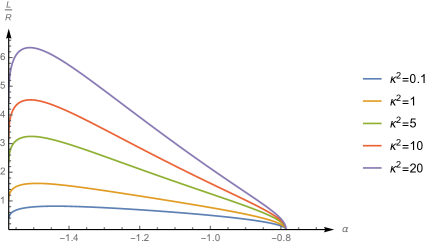
Figure 14: The behavior of the distance from the defect as a function of $m$ at $\chi=\frac{\pi}{2}$ is not qualitatively different from the one obtained for other values of the angle greater than $\chi_{s}$. All the curves display a maximum.

with the combination $\sqrt{n}\tilde{\sigma}$ seen as a function of $m$ is given in eq. (D.2). The behavior of the distance with $m$ is then displayed in fig. 14 where as usual we have parametrized $m$ as $\tan\alpha.$ All the curves (independently of the value of the flux) are not monotonic function of $m$ and display a maximum, which becomes steeper as the flux increases. The distance from the defect always vanishes at $m=-1$. This property can be checked analytically by means of the results of app. A. Next we examine the area given by eq. (3.13). Its behavior is pictured in fig. 16 and we again find that it is not a monotonic function of $m$. When $\alpha=\arctan(m)$ increases, it reaches a maximum exactly for the same value of $\alpha$ for which the distance does and then it decreases to $-\infty$. For $\alpha=-\frac{\pi}{2}$, namely $m\to-\infty$ all the curves go to the same value: in this case $-1$. Therefore we observe the same behavior previously obtained for all the angles $\chi>\chi_{s}$.

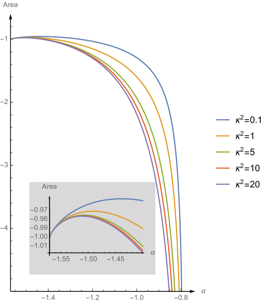
Figure 15: The behavior of the area of the connected surface as a function of $m$ at $\chi=\frac{\pi}{2}$ is not qualitatively different from the other values of the angle greater than $\chi_{s}$. All the curves display a maximum

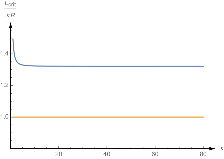
Figure 16: Plot of $\frac{L_{\rm cric.}}{\kappa R}$ as function of $\kappa$. This quantity is decreasing with the flux, but always greater than one.

Finally, we investigate the phase transition from the dome to the connected solution when we vary the distance from the defect. For $\chi=\frac{\pi}{2}$ the disconnected solution cannot exist for all distances. In fact, when $\frac{L}{\kappa R}<1$, the dome solution is no more acceptable because it intersects the (defect) brane. This phenomenus could provides a second putative mechanism for the phase transition from a disconnected to a connected minimal surface: even if the area of the latter might become dominant only when $\frac{L}{\kappa R}<1$, we are forced to start using it at $\frac{L}{\kappa R}=1$. In this case the transition is of order zero.

However this second mechanism remains inoperative if the area of the connected solutions becomes smaller than $-1$ before the dome touches the brane. To explore this point we have plotted in fig. 16 the critical distance divided by $\kappa R$ for different values of the flux. This quantity is monotonically decreasing with $\kappa$, but it is always greater than one. Thus the first-order transition always occurs before the dome touches the brane.

Appendix E Connected solution as correlator between two circles of different radii

In this appendix we show that our extremal surface can be viewed as the solution connecting two coaxial circles of different radii and different couplings with the scalars. The former is identified with the original one. The latter is located behind the defect, and the distance from it is chosen so that the brane intersects the extremal surface orthogonally.

To begin with, we shall examine more carefully the geometric structure of our solution. In $AdS_{5}$ our connected solution is given by

$$\begin{gathered}y(\sigma)=\frac{R\cosh\eta}{\sqrt{1+g^{2}(\sigma)}}\textrm{sech}[v(\sigma)-\eta]\quad\quad r(\sigma)=R\cosh\eta\frac{g(\sigma)}{\sqrt{1+g^{2}(\sigma)}}\textrm{sech}[v(\sigma)-\eta]\\ x_{3}(\sigma)=-R\cosh\eta\tanh[v(\sigma)-\eta],\end{gathered}$$ (E.1)

and it is confined into a $S^{3}$ inside AdS₅. In fact

$$\begin{split}x^{2}+y^{2}+r^{2}=&R^{2}\cosh^{2}\eta\left[\frac{\textrm{sech}^{2}[v(\sigma)-\eta]}{1+g^{2}(\sigma)}+\frac{g^{2}(\sigma)}{1+g^{2}(\sigma)}\textrm{sech}^{2}[v(\sigma)-\eta]+\tanh^{2}[v(\sigma)-\eta]\right]=\\ =&R^{2}\cosh^{2}\eta=\sqrt{L^{2}+R^{2}}\end{split}$$ (E.2)

The surface (E.1) intersects the boundary of AdS₅ at $\sigma=0$ and if we extend the range of the world-sheet coordinate $\sigma$ beyond $\tilde{\sigma}$, it reaches again the boundary at $\hat{\sigma}=\frac{1}{\sqrt{n}}\mathds{K}(m)$ for which

$$v(\hat{\sigma})=2\sqrt{\frac{\epsilon_{0}}{n}}\left[\mathds{K}(m)-\Pi\left(-\frac{1}{n},m\right)\right].$$ (E.3)

This second intersection with the boundary of AdS₅ is again a circle of radius

$$\hat{R}=R\cosh\eta~{}\textrm{sech}\left(2\sqrt{\frac{\epsilon_{0}}{n}}\left[\mathds{K}(m)-\Pi\left(-\frac{1}{n},m\right)\right]-\eta\right).$$ (E.4)

This second circle is located at

$$\begin{split}x_{3}(\hat{\sigma})=&-R\cosh\eta\tanh[v(\hat{\sigma})-\eta]=R\sinh\eta-R\sinh v(\hat{\sigma})\textrm{sech}\left(v(\hat{\sigma})-\eta\right)=\\ =&R\sinh\eta-\hat{R}\textrm{sech}\eta\sinh v(\hat{\sigma})\end{split}$$ (E.5)

and the distance $\ell$ in the transverse direction $x_{3}$ between this circle and the one at $\sigma=0$ is

$$\ell=\hat{R}\textrm{sech}\eta\sinh v(\hat{\sigma}).$$ (E.6)

The angle $\chi$ describing the scalars coupling to the two circles is different and the $\Delta\chi$ between the two loops is

$$\Delta\chi=\theta(\hat{\sigma})-\theta(0)=\frac{2j}{\sqrt{n}}\mathds{K}(m).$$ (E.7)

Appendix F Basis for chiral primary operators

As already pointed out in the original papers, the only operators built from scalars that can have one-point functions different from zero are those invariant under $SO(3)\times SO(3)$. If we consider the case of operator with classical dimension $2$ we can construct only two operators of this type: the famous Konishi operator

$$\mathcal{K}(x)=\frac{4\pi^{2}}{\sqrt{3}}\mathrm{Tr}(\Phi_{I}\Phi^{I})$$ (F.1)

and the chiral primary operator

$$\mathfrak{O}_{1}(x)=\sqrt{\frac{1}{6}}\mathrm{Tr}\left[\Phi_{1}^{2}+\Phi_{2}^{2}+\Phi_{3}^{2}-\Phi_{4}^{2}-\Phi_{5}^{2}-\Phi_{6}^{2}\right].$$ (F.2)

The list of CPO’s is completed by $4$ diagonal operators

$$\begin{split}\mathfrak{O}_{2}(x)=\sqrt{\frac{1}{2}}\mathrm{Tr}\left[\Phi_{1}^{2}-\Phi_{3}^{2}\right]\ \ \ \ \ \ \ \mathfrak{O}_{3}(x)=\sqrt{\frac{1}{6}}\mathrm{Tr}\left[\Phi_{1}^{2}-2\Phi_{2}^{2}+\Phi_{3}^{2}\right]\\ \mathfrak{O}_{4}(x)=\sqrt{\frac{1}{2}}\mathrm{Tr}\left[\Phi_{4}^{2}-\Phi_{6}^{2}\right]\ \ \ \ \ \ \ \mathfrak{O}_{5}(x)=\sqrt{\frac{1}{6}}\mathrm{Tr}\left[\Phi_{4}^{2}-2\Phi_{5}^{2}+\Phi_{6}^{2}\right]\end{split}$$ (F.3)

and $15$ off-diagonal ones $\mathfrak{O}_{IJ}(x)=\sqrt{2}\mathrm{Tr}\left[\Phi_{I}\Phi_{J}\right]$ with $i<j$. When performing integrability calculation, one usually computes the expectation values of the CPO $\mathrm{Tr}(Z^{2})$. We want to expand this operator in our basis and we find

$$\begin{split}\mathrm{Tr}(Z^{2})=&\mathrm{Tr}(\Phi_{3}^{2}-\Phi_{6}^{2})+2i\mathrm{Tr}(\Phi_{3}\Phi_{6})=\\ =&\sqrt{\frac{2}{3}}\mathfrak{O}_{1}(x)-\sqrt{\frac{1}{2}}\mathfrak{O}_{2}(x)+\sqrt{\frac{1}{6}}\mathfrak{O}_{3}(x)+\sqrt{\frac{1}{2}}\mathfrak{O}_{4}(x)-\sqrt{\frac{1}{6}}\mathfrak{O}_{5}(x)+\sqrt{2}i\mathfrak{O}_{36}(x).\end{split}$$ (F.4)

Then we have the following relation between the VEV’s:

$$\langle\mathfrak{O}_{1}(x)\rangle_{0}=\sqrt{\frac{3}{2}}\langle\mathrm{Tr}(Z^{2})\rangle_{0}.$$ (F.5)

Actually in the Wilson loop operator appears the following linear combination of CPO $Y^{a}(\theta)\mathcal{O}_{a}(x)$, where $Y^{a}(\theta)=(C^{a}_{IJ}\theta^{I}\theta^{J})=\left(-\sqrt{\frac{1}{6}},0,0,-\sqrt{\frac{1}{2}},\sqrt{\frac{1}{6}},\mathbf{0}\right)$ is a $20$ component vector. The boldface zero indicates that the remaining $15$ components vanishes and the $C^{a}_{IJ}$ form the basis of the symmetric traceless tensors that we used for constructing the CPO. Then

$$\langle Y^{a}(\theta)\mathcal{O}_{a}(x)\rangle=\langle Y^{1}(\theta)\mathcal{O}_{1}(x)\rangle=4\sqrt{2}\pi^{2}\langle Y^{1}(\theta)\mathfrak{O}_{1}(x)\rangle=-\frac{4\pi^{2}}{\sqrt{2}}\langle\mathrm{Tr}(Z^{2})\rangle$$ (F.6)

Now if we use eq. (28) of Buhl-Mortensen:2017ind , we find up to one-loop

$$\begin{split}\langle\mathrm{Tr}(Z^{2})\rangle=&-\frac{1}{12L^{2}}k(1-k^{2})\!+\!\frac{g^{2}_{YM}}{8\pi^{2}L^{2}}\left(k(N-k)\!+\!\frac{(k-1)}{2}\!+\!\sum^{\left[\frac{k-2}{2}\right]}_{i=0}(H_{k-i-1}-H_{i})(k-2i-1)\right)=\\ =&-\frac{1}{12L^{2}}k(1-k^{2})+\frac{g^{2}_{YM}}{8\pi^{2}L^{2}}\left(k(N-k)+\frac{(k-1)}{2}+\frac{k(k-1)}{2}\right)=\\ =&-\frac{1}{12L^{2}}k(1-k^{2})+\frac{g^{2}_{YM}}{8\pi^{2}L^{2}}\left(k(N-k)+\frac{k^{2}-1}{2}\right)\end{split}$$ (F.7)

Therefore

$$\langle Y^{a}(\theta)\mathcal{O}_{a}(x)\rangle=-\frac{4\pi^{2}}{\sqrt{2}}\langle\mathrm{Tr}(Z^{2})\rangle=\frac{\pi^{2}}{3\sqrt{2}L^{2}}k(1-k^{2})-\frac{g^{2}_{YM}}{2\sqrt{2}L^{2}}\left(k(N-k)+\frac{k^{2}-1}{2}\right)$$ (F.8)

For the Konishi operator up to one-loop instead we have Buhl-Mortensen:2017ind

$$\langle\mathcal{K}(x)\rangle=-\frac{\pi^{2}}{\sqrt{3}L^{2}}k(1-k^{2})-\frac{\sqrt{3}\lambda}{4L^{2}}k\left(1-k^{2}\right)\left(\psi\left(\frac{k+1}{2}\right)+\gamma_{E}-\log 2+\frac{5}{6}\right)$$ (F.9)

References

- (1) A. Karch and L. Randall, Localized gravity in string theory, Phys. Rev. Lett. 87 (2001) 061601, [hep-th/0105108].
- (2) A. Karch and L. Randall, Open and closed string interpretation of SUSY CFT’s on branes with boundaries, JHEP 06 (2001) 063, [hep-th/0105132].
- (3) O. DeWolfe, D. Z. Freedman and H. Ooguri, Holography and defect conformal field theories, Phys. Rev. D66 (2002) 025009, [hep-th/0111135].
- (4) J. Erdmenger, Z. Guralnik and I. Kirsch, Four-dimensional superconformal theories with interacting boundaries or defects, Phys. Rev. D66 (2002) 025020, [hep-th/0203020].
- (5) K. Nagasaki, H. Tanida and S. Yamaguchi, Holographic Interface-Particle Potential, JHEP 01 (2012) 139, [1109.1927].
- (6) I. Buhl-Mortensen, M. de Leeuw, A. C. Ipsen, C. Kristjansen and M. Wilhelm, One-loop one-point functions in gauge-gravity dualities with defects, Phys. Rev. Lett. 117 (2016) 231603, [1606.01886].
- (7) K. Nagasaki and S. Yamaguchi, Expectation values of chiral primary operators in holographic interface CFT, Phys. Rev. D86 (2012) 086004, [1205.1674].
- (8) C. Kristjansen, G. W. Semenoff and D. Young, Chiral primary one-point functions in the D3-D7 defect conformal field theory, JHEP 01 (2013) 117, [1210.7015].
- (9) I. Buhl-Mortensen, M. de Leeuw, A. C. Ipsen, C. Kristjansen and M. Wilhelm, A Quantum Check of AdS/dCFT, JHEP 01 (2017) 098, [1611.04603].
- (10) M. de Leeuw, C. Kristjansen and K. Zarembo, One-point Functions in Defect CFT and Integrability, JHEP 08 (2015) 098, [1506.06958].
- (11) I. Buhl-Mortensen, M. de Leeuw, C. Kristjansen and K. Zarembo, One-point Functions in AdS/dCFT from Matrix Product States, JHEP 02 (2016) 052, [1512.02532].
- (12) I. Buhl-Mortensen, M. de Leeuw, A. C. Ipsen, C. Kristjansen and M. Wilhelm, Asymptotic One-Point Functions in Gauge-String Duality with Defects, Phys. Rev. Lett. 119 (2017) 261604, [1704.07386].
- (13) M. de Leeuw, A. C. Ipsen, C. Kristjansen, K. E. Vardinghus and M. Wilhelm, Two-point functions in AdS/dCFT and the boundary conformal bootstrap equations, JHEP 08 (2017) 020, [1705.03898].
- (14) S.-J. Rey and J.-T. Yee, Macroscopic strings as heavy quarks in large N gauge theory and anti-de Sitter supergravity, Eur. Phys. J. C22 (2001) 379–394, [hep-th/9803001].
- (15) J. M. Maldacena, Wilson loops in large N field theories, Phys. Rev. Lett. 80 (1998) 4859–4862, [hep-th/9803002].
- (16) K. Zarembo, Localization and AdS/CFT Correspondence, J. Phys. A50 (2017) 443011, [1608.02963].
- (17) J. K. Erickson, G. W. Semenoff and K. Zarembo, Wilson loops in N=4 supersymmetric Yang-Mills theory, Nucl. Phys. B582 (2000) 155–175, [hep-th/0003055].
- (18) N. Drukker and D. J. Gross, An Exact prediction of N=4 SUSYM theory for string theory, J. Math. Phys. 42 (2001) 2896–2914, [hep-th/0010274].
- (19) V. Pestun, Localization of gauge theory on a four-sphere and supersymmetric Wilson loops, Commun. Math. Phys. 313 (2012) 71–129, [0712.2824].
- (20) M. de Leeuw, A. C. Ipsen, C. Kristjansen and M. Wilhelm, One-loop Wilson loops and the particle-interface potential in AdS/dCFT, Phys. Lett. B768 (2017) 192–197, [1608.04754].
- (21) J. Aguilera-Damia, D. H. Correa and V. I. Giraldo-Rivera, Circular Wilson loops in defect Conformal Field Theory, JHEP 03 (2017) 023, [1612.07991].
- (22) M. Preti, D. Trancanelli and E. Vescovi, Quark-antiquark potential in defect conformal field theory, JHEP 10 (2017) 079, [1708.04884].
- (23) N. Drukker, S. Giombi, R. Ricci and D. Trancanelli, Supersymmetric Wilson loops on S**3, JHEP 05 (2008) 017, [0711.3226].
- (24) S. Giombi, V. Pestun and R. Ricci, Notes on supersymmetric Wilson loops on a two-sphere, JHEP 07 (2010) 088, [0905.0665].
- (25) A. Bassetto, L. Griguolo, F. Pucci, D. Seminara, S. Thambyahpillai and D. Young, Correlators of supersymmetric Wilson-loops, protected operators and matrix models in N=4 SYM, JHEP 08 (2009) 061, [0905.1943].
- (26) N. R. Constable, R. C. Myers and O. Tafjord, The noncommutative bion core, Phys.Rev.D 61 (2000) 106009, [hep-th/9911136].
- (27) H. Kim, D. K. Park, S. Tamarian and H. J. W. Muller-Kirsten, Gross-Ooguri phase transition at zero and finite temperature: Two circular Wilson loop case, JHEP 03 (2001) 003, [hep-th/0101235].
- (28) “NIST Digital Library of Mathematical Functions.” http://dlmf.nist.gov/, Release 1.0.24 of 2019-09-15.
- (29) D. E. Berenstein, R. Corrado, W. Fischler and J. M. Maldacena, The operator product expansion for wilson loops and surfaces in the large n limit, Phys.Rev.D 59 (1999) 105023, [hep-th/9809188].
- (30) G. Arutyunov, J. Plefka and M. Staudacher, Limiting geometries of two circular Maldacena-Wilson loop operators, JHEP 12 (2001) 014, [hep-th/0111290].
- (31) K. Konishi, Anomalous Supersymmetry Transformation of Some Composite Operators in SQCD, Phys. Lett. 135B (1984) 439–444.
- (32) D. Anselmi, The N=4 quantum conformal algebra, Nucl. Phys. B541 (1999) 369–385, [hep-th/9809192].
- (33) M. Bianchi, S. Kovacs, G. Rossi and Y. S. Stanev, On the logarithmic behavior in N=4 SYM theory, JHEP 08 (1999) 020, [hep-th/9906188].
- (34) G. Arutyunov, S. Frolov and A. C. Petkou, Operator product expansion of the lowest weight CPOs in SYM4 at strong coupling, Nucl. Phys. B586 (2000) 547–588, [hep-th/0005182].
- (35) G. Arutyunov, S. Frolov and A. Petkou, Perturbative and instanton corrections to the OPE of CPOs in SYM4, Nucl. Phys. B602 (2001) 238–260, [hep-th/0010137].
- (36) G. Arutyunov, B. Eden, A. Petkou and E. Sokatchev, Exceptional nonrenormalization properties and ope analysis of chiral four point functions in n=4 sym(4), Nucl.Phys.B 620 (2002) 380–404, [hep-th/0103230].
- (37) S. Penati and A. Santambrogio, Superspace approach to anomalous dimensions in n=4 sym, Nucl.Phys.B 614 (2001) 367–387, [hep-th/0107071].
- (38) G. W. Semenoff and K. Zarembo, More exact predictions of SUSYM for string theory, Nucl. Phys. B616 (2001) 34–46, [hep-th/0106015].
- (39) S. Lee, S. Minwalla, M. Rangamani and N. Seiberg, Three point functions of chiral operators in D = 4, N=4 SYM at large N, Adv. Theor. Math. Phys. 2 (1998) 697–718, [hep-th/9806074].
- (40) A. C. Ipsen and K. E. Vardinghus, The dilatation operator for defect conformal SYM, 1909.12181.
- (41) S. Bonansea and R. Sanchéz, in preparation, 19xx.xxxx.