Data-driven Linear Quadratic Regulation via Semidefinite Programming

Abstract

This paper studies the finite-horizon linear quadratic regulation problem where the dynamics of the system are assumed to be unknown and the state is accessible. Information on the system is given by a finite set of input-state data, where the input injected in the system is persistently exciting of a sufficiently high order. Using data, the optimal control law is then obtained as the solution of a suitable semidefinite program. The effectiveness of the approach is illustrated via numerical examples.

1 Introduction

Optimization and control have always been closely related when there is need for operating a dynamical system at minimum cost. When the system is linear and the cost function is quadratic, the optimal control problem amounts to solving the popular linear quadratic regulator (LQR) problem (Anderson and Moore, 2007), whose duality with convex optimization is shown in Balakrishnan and Vandenberghe (1995) for continuous-time systems and more recently in Gattami (2009); Lee and Hu (2016) for discrete-time systems. The common assumption for deriving the solution is that an exact model of the system is available.

To cope with the lack of prior knowledge of the system dynamics, various control techniques have been developed. The classic approach is the so-called indirect approach: a model is first determined from data, and then the control law is designed using the model. It is worth to mention that the control objectives are not taken into account in the identification step and, once the model is derived from data, the data is not used in the synthesis of the control law. More recently, as opposed to the model-based paradigm, data-driven control, also termed model-free, has become increasingly popular. Data-driven control is based on the paradigm of learning a controller directly from data collected from the system. Various efforts have been made in this direction, in the context of optimal control for linear systems (Markovsky and Rapisarda, 2007; Gonçalves da Silva et al., 2018; Baggio et al., 2019; Coulson et al., 2019) as well as for designing control laws for nonlinear systems (Fliess and Join, 2013; Kaiser et al., 2017; Safonov and Tsao, 1994). Data-driven control has also been approached using popular Machine Learning tools such as Reinforcement Learning (RL). In RL (Sutton and Barto, 2018; Ten Hagen and Kröse, 1998; Bradtke et al., 1994), also referred to as approximate dynamic programming (Lewis et al., 2012; Busoniu et al., 2017), the controller learns an optimal policy through trial-and-error, trying to estimate a long-term value function. Other data-driven techniques are discussed in the surveys Benosman (2018); Hou and Wang (2013) to which the interested reader is referred. Despite advances in this area, data-driven control still poses many theoretical and practical challenges. For instance, in applications involving on-line control design, approaches like RL might suffer from the large number of iterations required to achieve convergence (Görges, 2017).

In this paper, we consider the finite-horizon LQR problem for linear time-invariant discrete-time systems. Different from the mainstream approaches based on RL techniques (Zhao et al., 2015; Pang et al., 2018; Liu et al., 2016), the approach we propose does not involve iterations. We formulate the LQR problem as a (one-shot) semidefinite program in which the model of the system is replaced by a finite number of data collected from the system. This idea has been proposed in De Persis and Tesi (2019) for the infinite-horizon LQR problem. The method proposed in this paper also recovers the infinite-horizon solution in a very natural way.

Our approach is based on the framework developed in De Persis and Tesi (2019), whose foundation lies on the fundamental lemma by Willems et al. (2005). Roughly speaking, the fundamental lemma stipulates that one can describe all possible trajectories of a linear time-invariant system using any given finite set of its input-output data, provided that these data come from sufficiently excited dynamics. This result thus establishes that data implicitly give a non-parametric system representation which can be directly used for control design.

The paper is organized as follows: Section 2 briefly reviews the model-based finite-horizon LQR solution. In Section 3, the LQR problem is reformulated as a convex optimization problem involving linear matrix inequalities (Boyd et al., 1994), resulting in a semidefinite program (SDP). The proposed approach is discussed in Section 3.2. We show that the data-based parametrization introduced in De Persis and Tesi (2019) combined with the SDP formulation of the LQR problem results in a direct parametrization of the feedback system through data. In turn, this makes it possible to determine the optimal control law in one-shot, with no intermediate identification step. Numerical examples are discussed in Section 4. The paper ends with some concluding remarks in Section 5.

Notation: Given a signal $z:\mathbb{Z}\rightarrow\mathbb{R}^{\sigma}$, we will denote by $z_{[i,k]}$ the sequence $\{z(i),\dots,z(k)\}$, where $i\leq k$. For a square matrix $A$, we denote by $\mathbf{Tr}(A)$ its trace. In addition, we write $A\succ 0$ and $A\succeq 0$ to denote that $A$ is positive definite (semi-definite). We use the notation $w(k)\sim\mathcal{N}(0,W)$ to represent a zero-mean Gaussian random vector such that $\mathbf{E}[w(k)]=0$ and $\mathbf{E}[w(k)w^{\top}(k)]=W$, where $\mathbf{E}$ denotes the expectation.

2 Finite-horizon LQR problem

Consider a discrete-time linear system

$$x(k+1)=Ax(k)+Bu(k)$$ (1)

where $x\in\mathbb{R}^{n}$ is the state while $u\in\mathbb{R}^{m}$ is the control input, and where $A$ and $B$ are matrices of an appropriate dimension. It is assumed throughout the paper that $(A,B)$ is controllable and the state is available for measurements. Given an initial condition $x(0)=x_{0}$ and a control sequence $u_{[0,N-1]}=\{u(0),\ \dots,\ u(N-1)\}$ over the horizon $N\in\mathbb{N}$, we consider the quadratic cost $J$ associated to system (1) starting at $x_{0}$,

$$J:=x(N)^{\top}Q_{f}x(N)+\sum_{k=0}^{N-1}\rho(u(k),x(k))$$ (2)

where

$$\rho(u,x)=x^{\top}Q_{x}x+u^{\top}Ru,$$

where $Q_{x},Q_{f}\succeq 0$ and $R\succ 0$. The finite-horizon linear quadratic regulator (LQR) problem is as follows:

Problem 1

Given system (1) with initial condition $x_{0}$, and given a time horizon of length $N$, find an input sequence such that the cost function (2) is minimized, i.e. solve the minimization problem:

$$\begin{array}[]{rl}\min_{\mu_{k}}&\,\,J\\[8.5359pt] \text{subject to }&\,\,x(k+1)=Ax(k)+Bu(k)\\[2.84544pt] &\,\,u(k)=\mu_{k}(x(0),x(1),\ldots,x(k)).\end{array}$$ (4)

Here, the last constraint means that the control input is a causal function of the system state.

The following result holds.

Lemma 1

For Problem 1, the optimal control sequence $u^{*}_{[0,N-1]}=\{u^{*}(0),\ \dots,\ u^{*}(N-1)\}$ is unique, and it is generated by the feedback law

$$u^{*}(k)=K^{*}(k)x(k)$$ (5)

where

$$K^{*}(k):=-(R+B^{\top}P(k+1)B)^{-1}B^{\top}P(k+1)A$$ (6)

where $P(k)$ is the solution to the so-called discrete-time difference Riccati equation

$$\begin{split}P&(k)=Q_{x}+A^{\top}P(k+1)A-\\ &A^{\top}P(k+1)B(R+B^{\top}P(k+1)B)^{-1}B^{\top}P(k+1)A\end{split}$$

initialized from $P(N)=Q_{f}$.

See for instance Bertsekas (1995). $\Box$ The computed control law (6) is time-varying and defined in the interval $[0,N]$. However, the computation of the gain $K^{*}(k)$ does not require the knowledge of the current state, and can be computed offline. For $N\rightarrow\infty$, if the pair $(Q_{x},A)$ is observable, the sequence of the matrices $P(k)$ converges to a matrix $P$, which is the so-called stabilizing solution of the discrete-time algebraic Riccati equation

$$P=Q_{x}+A^{\top}PA-A^{\top}PB(R+B^{\top}PB)^{-1}B^{\top}PA.$$

In this case, the optimal control for the infinite-horizon problem is a time-invariant state-feedback $u(k)=K^{*}x(k)$ with $K^{*}=-(R+B^{\top}PB)^{-1}B^{\top}PA$.

Remark 1

Here, similarly to the data-driven infinite-horizon LQR problem studied in De Persis and Tesi (2019), we have assumed that the pair $(A,B)$ is controllable. As discussed in Section 3, this assumption ensures that we can always collect sufficiently rich data by applying exciting input signals. As shown in van Waarde et al. (2019), except for pathological cases, data richness is indeed necessary for the data-driven solution of the LQR problem. On the other hand, data richness is also necessary for reconstructing the system matrices $A$ and $B$ from data, thus necessary also for the model-based solution whenever $A$ and $B$ have to be identified from data.

2.1 Solution as a covariance optimization problem

For reasons which will become clear in the next section, we introduce an equivalent formulation of the LQR problem, where by “equivalent” we mean that the corresponding optimal solution is still given by (5).

Consider the linear quadratic stochastic control problem (Gattami, 2009):

$$\begin{array}[]{rl}\min_{\mu_{k}}&\,\,\mathbf{E}[J]\\[8.5359pt] \text{subject to }&\,\,x(k+1)=Ax(k)+Bu(k)+w(k)\\[2.84544pt] &\,\,x(0)\sim\mathcal{N}(0,I_{n})\\[2.84544pt] &\,\,w(k)\sim\mathcal{N}(0,I_{n})\\[2.84544pt] &\,\,\mathbf{E}[w(k)x^{\top}(l)]=0,\quad\forall l\leq k\\[2.84544pt] &\,\,u(k)=\mu_{k}(x(0),x(1),\ldots,x(k))\end{array}$$ (8)

with $J$ as in (2). As detailed in Gattami (2009), this problem is equivalent to the covariance selection problem

$$\begin{array}[]{rl}&\min_{V(0),\ldots,V(N)\succeq 0}\ \mathbf{Tr}\,(Q_{f}S(N))+\sum_{k=0}^{N-1}\mathbf{Tr}(Q_{x}S(k)+R\,U(k))\\[8.5359pt] &\qquad\text{subject to }\\[5.69046pt] &\qquad S(0)=I_{n}\\[2.84544pt] &\qquad S(k+1)-\begin{bmatrix}A&&B\end{bmatrix}V(k)\begin{bmatrix}A&&B\end{bmatrix}^{\top}-I_{n}=0\\[2.84544pt] \end{array}$$ (13)

for $k=0,\ldots,N-1$, where

$$V(k)=\begin{bmatrix}S(k)&&Y(k)\\ Y(k)^{\top}&&U(k)\end{bmatrix}:=\mathbf{E}\begin{bmatrix}x(k)\\ u(k)\end{bmatrix}\begin{bmatrix}x(k)\\ u(k)\end{bmatrix}^{\top}.$$ (14)

In particular, the following result holds.

Theorem 1

(Gattami, 2009, Theorem 2) The optimal solution of the covariance selection problem (13) is given by

$$S(0)=I_{n}$$

$$Y(k)^{\top}=L(k)S(k)$$

$$U(k)=Y(k)^{\top}S^{-1}(k)Y(k)$$

$$S(k+1)=\begin{bmatrix}A&&B\end{bmatrix}V(k)\begin{bmatrix}A&&B\end{bmatrix}^{\top}+I_{n}.$$

The corresponding optimal control law is $u(k)=L(k)x(k)$ with $L(k)=K^{*}(k)$ as in (5).

3 Data-driven LQR via Semidefinite Programming

Building on the formulation described in Section 2.1, it is possible to derive a simple solution to the LQR problem where the system matrices $A$ and $B$ are replaced by data. We first show how the covariance optimization problem can be restated in terms of a semidefinite program. Then, we consider a parametrization of the feedback system which results in a pure data-driven formulation.

3.1 Semidefinite Programming formulation

The following result holds.

Theorem 2

The optimal control law for problem (13) can be computed as the solution $\mathcal{K}$ to the problem

$$\begin{array}[]{rl}&\min_{\mathcal{S},\mathcal{K},\mathcal{Z}}\ \mathbf{Tr}(Q_{f}S(N))+\sum_{k=0}^{N-1}\mathbf{Tr}(Q_{x}S(k)+Z(k))\\[8.5359pt] &\,\,\,\,\text{subject to }\\[8.5359pt] &\,\,\,\,S(0)\succeq I_{n}\\[2.84544pt] &\,\,\,\,S(k+1)-(A+BK(k))S(k)(A+BK(k))^{\top}-I_{n}\succeq 0\\[2.84544pt] &\,\,\,\,Z(k)-R^{1/2}K(k)S(k)K(k)^{\top}R^{1/2}\succeq 0\\[2.84544pt] \end{array}$$ (20)

for $k=0,\ldots,N-1$, where

$$\mathcal{S} :=\{S(1),\dots,S(N)\}$$

$$\mathcal{K} :=\{K(0),\dots,K(N-1)\}$$

$$\mathcal{Z} :=\{Z(0),\dots,Z(N-1)\}$$

Exploiting the fact that the optimal control law takes the form $u(k)=K(k)x(k)$, the term $\mathbf{Tr}(R\,U(k))$ appearing in the objective function of (13) can be written as

$$\mathbf{Tr}(R\,U(k)) = \mathbf{Tr}\,(R\,\mathbf{E}[K(k)x(k)x(k)^{\top}K(k)^{\top}])$$

$$= \mathbf{Tr}\,(R^{1/2}K(k)S(k)K(k)^{\top}R^{1/2}).$$

In addition,

$$V(k)=\begin{bmatrix}I\\ K(k)\end{bmatrix}S(k)\begin{bmatrix}I\\ K(k)\end{bmatrix}^{\top}$$

so that the second constraint of (13) becomes

$$S(k+1)-(A+BK(k))S(k)(A+BK(k))^{\top}+I_{n}=0.$$

Accordingly, the optimization problem (13) is equivalent to the following problem:

$$\begin{array}[]{rl}&\min_{\mathcal{S},\mathcal{K},\mathcal{Z}}\ \mathbf{Tr}(Q_{f}S(N))+\sum_{k=0}^{N-1}\mathbf{Tr}(Q_{x}S(k)+Z(k))\\[8.5359pt] &\,\,\,\,\text{subject to }\\[8.5359pt] &\,\,\,\,S(0)=I_{n}\\[2.84544pt] &\,\,\,\,S(k+1)-(A+BK(k))S(k)(A+BK(k))^{\top}-I_{n}=0\\[2.84544pt] &\,\,\,\,Z(k)-R^{1/2}K(k)S(k)K(k)^{\top}R^{1/2}=0\\[2.84544pt] \end{array}$$ (26)

Finally, let $(\overline{}\mathcal{S},\overline{}\mathcal{K},\overline{}\mathcal{Z})$ be an optimal solution to problem (20) and let $(\mathcal{S}^{*},\mathcal{K}^{*},\mathcal{Z}^{*})$ be an optimal solution to (26), where $\mathcal{K}^{*}=\{K^{*}(0),\dots,K^{*}(N-1)\}$ is the optimal sequence of state-feedback matrices given by (5). Also, denote by $\overline{J}$ and $J^{*}$ the corresponding costs. Clearly $\overline{J}\leq J^{*}$ since (20) has a larger feasible set than (26). To prove the converse inequality, first note that $\overline{S}(k)\succeq S^{*}(k)$ and $\overline{Z}(k)\succeq Z^{*}(k)$ for all $k\geq 0$. This follows because $\overline{S}(0)\succeq S^{*}(0)$ and since $\overline{S}(k)\succeq S^{*}(k)$ implies

$$(A+BK(k))\left(\overline{S}(k)-S^{*}(k)\right)(A+BK(k))^{\top}\succeq 0$$

$$R^{1/2}K(k)\left(\overline{S}(k)-S^{*}(k)\right)K(k)^{\top}R^{1/2}\succeq 0.$$

Substituting $(\overline{}\mathcal{S},\overline{}\mathcal{Z})$ in (20) and $(\mathcal{S}^{*},\mathcal{Z}^{*})$ in (26), we thus have $\overline{J}\geq J^{*}$ so that $\overline{J}=J_{*}$. In turn, this implies $\overline{}\mathcal{K}=\mathcal{K}^{*}$ since the optimal control law achieving $J^{*}$ is unique. $\Box$

Defining $H(k)=K(k)S(k)$ and using the property that $S(k)\succeq I_{n}$ for every $k\geq 0$, problem (20) can be converted into a semidefinite program. The idea of resorting to SDP formulations has been originally proposed in Feron et al. (1992) in the context of model-based LQR, and considered in De Persis and Tesi (2019) in the context of data-driven infinite-horizon LQR.

3.2 Data-driven parametrization of LQR

The formulation (20) is very appealing from the perspective of computing the control law using data only since the decision variables $\mathcal{S}$, $\mathcal{K}$ and $\mathcal{Z}$ appearing in (20) enter the problem in a form which permits to write the constraints as data-dependent linear matrix inequalities.

Our approach uses the concept of persistence of excitation, which is recalled via the following definitions.

Definition 1

Given a signal $z\in\mathbb{R}^{\sigma}$, we denote its Hankel matrix as

$$Z_{i,\ell,j}:=\begin{bmatrix}z(i)&z(i+1)&\cdots&z(i+j-1)\\ z(i+1)&z(i+2)&\cdots&z(i+j)\\ \vdots&\vdots&\ddots&\vdots\\ z(i+\ell-1)&z(i+\ell)&\cdots&z(i+\ell+j-2)\\ \end{bmatrix}$$

where $i\in\mathbb{Z}$ and $\ell,j\in\mathbb{N}$. If $\ell=1$, we denote its Hankel matrix as

$$Z_{i,j}=\begin{bmatrix}z(i)&z(i+1)&\cdots&z(i+j-1)\end{bmatrix}.$$

Definition 2

The signal $z_{[0,T-1]}:[0,T-1]\cap\mathbb{Z}\to\mathbb{R}^{\sigma}$ is said to be persistently exciting of order $\ell$ if the matrix $Z_{0,\ell,j}$, with $j=T-\ell+1$ has full rank $\sigma\ell$.

For a signal to be persistently exciting of order $\ell$, it must be sufficiently long in the sense that $T\geq(\sigma+1)\ell-1$.

Consider system (1),

$$x(k+1)=Ax(k)+Bu(k)$$

where $x\in\mathbb{R}^{n}$ and $u\in\mathbb{R}^{m}$. Suppose that we carried out an experiment of duration $T\in\mathbb{N}$, collecting input and state data $u_{d,[0,T]}$ and $x_{d,[0,T]}$ where the subscript “$d$” denotes data. Let the corresponding Hankel matrices be

$$\begin{split}U_{0,T}&:=\begin{bmatrix}u_{d}(0)&u_{d}(1)&\dots&u_{d}(T-1)\end{bmatrix}\\[2.84544pt] X_{0,T}&:=\begin{bmatrix}x_{d}(0)&x_{d}(1)&\dots&x_{d}(T-1)\end{bmatrix}\\[2.84544pt] X_{1,T}&:=\begin{bmatrix}x_{d}(1)&x_{d}(2)&\dots&x_{d}(T)\end{bmatrix}.\\[2.84544pt] \end{split}$$ (27)

Lemma 2

(Willems et al., 2005, Corollary 1) Suppose that system (1) is controllable. If the input signal $u_{d,[0,T-1]}$ is persistently exciting of order $n+1$ then

$$\begin{split}\text{rank}\begin{bmatrix}U_{0,T}\\[2.84544pt] X_{0,T}\end{bmatrix}=n+m.\end{split}$$ (28)

Remark 2

Condition (28) expresses the property that the data content is sufficiently rich, and this enables the data-driven solution of the LQR problem (cf. Remark 2). For a discussion on the types of persistently exciting signals the interested reader is referred to (Verhaegen and Verdult, 2007, Section 10).

A straightforward implication of the above result is that any input-state sequence of the system can be expressed as a linear combination of the collected input-state data. As shown in De Persis and Tesi (2019), one can use condition (28) also for parametrizing an arbitrary feedback interconnection. To see this, consider an arbitrary matrix $K(k)$, possibly time-varying, of dimension $m\times n$. By the Rouché-Capelli theorem, there exists a $T\times n$ matrix $G(k)$ solution to

$$\begin{bmatrix}K(k)\\[2.84544pt] I_{n}\end{bmatrix}=\begin{bmatrix}U_{0,T}\\[2.84544pt] X_{0,T}\end{bmatrix}G(k).$$ (29)

Accordingly the closed-loop system formed by system (1) with $u(k)=K(k)x(k)$ is such that

$$A+BK(k) = \begin{bmatrix}B&&A\end{bmatrix}\begin{bmatrix}K(k)\\[2.84544pt] I_{n}\end{bmatrix}$$ (30)

$$= \begin{bmatrix}B&&A\end{bmatrix}\begin{bmatrix}U_{0,T}\\[2.84544pt] X_{0,T}\end{bmatrix}G(k)$$

$$= X_{1,T}G(k)$$

where we used the identity $X_{1,T}=AX_{0,T}+BU_{0,T}$.

Using this result, one can provide a data-based formulation of problem (20).

Theorem 3

Consider system (1) along with an experiment of length $T\in\mathbb{N}$ resulting in input and state data $u_{d,[0,T]}$ and $x_{d,[0,T]}$, respectively. Let the matrices $U_{0,T}$, $X_{0,T}$ and $X_{1,T}$ be as in (27), and suppose that the rank condition (28) holds. Then, the optimal solution to problem (20), hence to Problem 1, is given by

$$\mathcal{K}:=\{K(0),\dots,K(N-1)\}$$

with

$$K(k)=U_{0,T}Q(k)S^{-1}(k)$$

where the matrices $Q(k)$ and $S(k)$ solve the optimization problem

$$\begin{array}[]{rl}&\min_{\mathcal{S},\mathcal{Q},\mathcal{Z}}\ \mathbf{Tr}(Q_{f}S(N))+\sum_{k=0}^{N-1}\mathbf{Tr}(Q_{x}S(k)+Z(k))\\[8.5359pt] &\quad\text{subject to }\\[8.5359pt] &\quad S(0)\succeq I_{n}\\[5.69046pt] &\quad S(k)=X_{0,T}Q(k)\\[5.69046pt] &\quad\begin{bmatrix}S(k+1)-I_{n}&&X_{1,T}Q(k)\\[2.84544pt] Q^{\top}(k)X_{1,T}^{\top}&&S(k)\end{bmatrix}\succeq 0\\[14.22636pt] &\quad\begin{bmatrix}Z(k)&&R^{1/2}U_{0,T}Q(k)\\[2.84544pt] Q(k)^{\top}U_{0,T}^{\top}R^{1/2}&&S(k)\end{bmatrix}\succeq 0\\[14.22636pt] \end{array}$$ (37)

for $k=0,\ldots,N-1$, where

$$\begin{split}\mathcal{S}&:=\{S(1),\dots,S(N)\}\\[2.84544pt] \mathcal{Q}&:=\{Q(0),\dots,Q(N-1)\}\\[2.84544pt] \mathcal{Z}&:=\{Z(0),\dots,Z(N-1)\}\end{split}$$ (38)

We show that the constraints of (20) can be written as in (37). To this end, first note that the parametrization (30) implies that the second constraint of (20) can also be written as

$$S(k+1)-X_{1,T}G(k)S(k)G(k)^{\top}X^{\top}_{1,T}-I_{n}\succeq 0$$

where $G(k)$ satisfies (29). Let now

$$Q(k):=G(k)S(k).$$ (39)

Exploiting the fact that $S(k)\succeq I_{n}$ for every $k\geq 0$ the second constraint of (20) becomes

$$S(k+1)-X_{1,T}Q(k)S^{-1}(k)Q(k)^{\top}X^{\top}_{1,T}-I_{n}\succeq 0$$

which is equivalent to the third constraint in (37). Along the same lines, the third constraint in (20) can be written as the fourth constraint in (37). Finally, the optimal solution $\mathcal{K}:=\{K(0),\dots,K(N-1)\}$, with $K(k)=U_{0,T}Q(k)S^{-1}(k)$, is obtained from the first one of (29) and (39). $\Box$

Remark 3

As $N\rightarrow\infty$ the solution converges to the infinite-horizon steady-state solution, which is stabilizing. The infinite-horizon formulation is discussed in De Persis and Tesi (2019).

4 Numerical examples

We consider both the semidefinite programs described in Theorem 2 (model-based) and Theorem 3 (data-driven) and compare their performance for randomly generated systems and for the batch reactor system.

4.1 Monte Carlo simulations on random systems

We perform Monte Carlo simulations with $N_{trials}=1000$ random systems with $3$ states and $1$ input. Simulations are performed in MATLAB. For each trial, the entries of the system matrices are generated using the command randn (normally distributed random number). For each trial, the data are generated by applying a random input sequence of length $T=15$ and random initial conditions, again using the command randn. Using CVX (Grant et al. (2008)), we solve the model-based program (20) and the data-driven program (37) for $N=10$ steps with $Q_{x}=Q_{f}=I_{3}$ and $R=1$, and measure the resulting optimal costs.

A shown in Figure 1, for each trial the data-driven solution achieves the same cost as the model-based solution, with an average error of order $10^{-7}$. Also the sequence $\mathcal{K}^{*}_{dd}$ of data-driven feedback gains coincides with the sequence $\mathcal{K}^{*}_{mb}$ obtained by solving the model-based formulation, with an average error over the various gains of order $10^{-6}$ (Figure 2).

Figure 1: Absolute error between optimal cost $J^{*(i)}_{mb}$ achieved in model-based and optimal cost $J^{*(i)}_{dd}$ achieved in data-driven for the $i$-th trial.

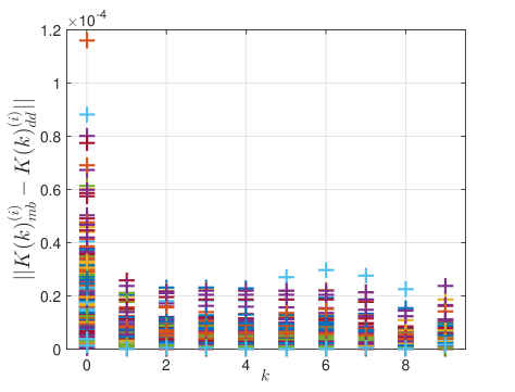
Figure 2: Values of the error (Euclidean norm) between the optimal model-based solutions $K(k)^{(i)}_{mb}$ and data-based solutions $K(k)^{(i)}_{dd}$ for the $i$-th trial, with $k=0,\dots,~{}N-1$.

4.2 Monte Carlo simulations on batch reactor system

As a second example, we consider the discretized version of the batch reactor system (Walsh and Ye, 2001), using a sampling time of $0.1s$,

$$\left[\begin{array}[]{c|c}A&B\end{array}\right]=$$ (41)

$$\quad\left[\begin{array}[]{rrrrc|crr}1.178&0.001&0.511&-0.403&&&0.004&-0.087\\ -0.051&0.661&-0.011&0.061&&&0.467&0.001\\ 0.076&0.335&0.560&0.382&&&0.213&-0.235\\ 0&0.335&0.089&0.849&&&0.213&-0.016\end{array}\right]$$ (46)

which is open-loop unstable.

Under the same experimental conditions as in the previous example ($T=15$, $N=10$, $N_{trials}=1000$), and taking cost weights $Q_{x}=Q_{f}=I_{4}$ and $R=I_{2}$, Monte Carlo simulations return an average error of order $10^{-3}$ for what concerns the discrepancy $|J^{*}_{dd}-J^{*}_{mb}|$, and an average error of order $10^{-3}$ for what concerns $\|\mathcal{K}^{*}_{dd}-\mathcal{K}^{*}_{mb}\|$.

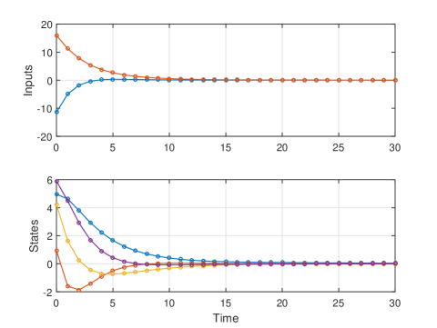
Figure 3: Optimal input sequence and state response with $N=30$ for the batch reactor system.

As $N$ grows the solution approximates the infinite-horizon steady-state solution, which is stabilizing. Figure 3 shows the closed-loop response with the data-driven solution for one experiment carried out with $N=30$.

5 Conclusions

We considered a finite-horizon linear quadratic regulation problem, where the knowledge about the dynamics of the system is replaced by a finite set of input and state data collected from an experiment. We have shown that if the experiment is carried out with a sufficiently exciting input signal then the optimal solution can be computed only using the data, with no intermediate identification step, as the result of a data-dependent semidefinite programming problem.

An important continuation of this research line involves the extension of these results to the case where data are affected by noise, also in comparison with techniques based on system identification (Dean et al., 2017). Concerning data-driven methods, previous efforts in this direction include De Persis and Tesi (2019) for stabilization in the presence of input disturbances and/or measurement noise, and Berberich et al. (2019), which considers robust performance (including $H_{\infty}$ control as a special case) in the presence of input disturbances.

References

- Anderson and Moore (2007) Anderson, B.D. and Moore, J.B. (2007). Optimal control: linear quadratic methods. Courier Corporation.
- Baggio et al. (2019) Baggio, G., Katewa, V., and Pasqualetti, F. (2019). Data-driven minimum-energy controls for linear systems. IEEE Control Systems Letters, 3(3), 589–594.
- Balakrishnan and Vandenberghe (1995) Balakrishnan, V. and Vandenberghe, L. (1995). Connections between duality in control theory and convex optimization. In Proceedings of 1995 American Control Conference-ACC’95, volume 6, 4030–4034. IEEE.
- Benosman (2018) Benosman, M. (2018). Model-based vs data-driven adaptive control: An overview. International Journal of Adaptive Control and Signal Processing, 32(5), 753–776.
- Berberich et al. (2019) Berberich, J., Romer, A., Scherer, C.W., and Allgöwer, F. (2019). Robust data-driven state-feedback design. arXiv preprint arXiv:1909.04314.
- Bertsekas (1995) Bertsekas, D.P. (1995). Dynamic Programming and Optimal Control, volume 1. Athena scientific Belmont, MA.
- Boyd et al. (1994) Boyd, S., El Ghaoui, L., Feron, E., and Balakrishnan, V. (1994). Linear matrix inequalities in system and control theory, volume 15. Siam.
- Bradtke et al. (1994) Bradtke, S.J., Ydstie, B.E., and Barto, A.G. (1994). Adaptive linear quadratic control using policy iteration. In Proceedings of 1994 American Control Conference-ACC’94, volume 3, 3475–3479. IEEE.
- Busoniu et al. (2017) Busoniu, L., Babuska, R., De Schutter, B., and Ernst, D. (2017). Reinforcement learning and dynamic programming using function approximators. CRC press.
- Coulson et al. (2019) Coulson, J., Lygeros, J., and Dörfler, F. (2019). Data-enabled predictive control: in the shallows of the DeePC. In 2019 18th European Control Conference (ECC), 307–312. IEEE.
- De Persis and Tesi (2019) De Persis, C. and Tesi, P. (2019). Formulas for data-driven control: Stabilization, optimality and robustness. arXiv preprint arXiv:1903.06842.
- Dean et al. (2017) Dean, S., Mania, H., Matni, N., Recht, B., and Tu, S. (2017). On the sample complexity of the linear quadratic regulator. arXiv preprint arXiv:1710.01688.
- Feron et al. (1992) Feron, E., Balakrishnan, V., Boyd, S., and El Ghaoui, L. (1992). Numerical methods for related problems. In 1992 American Control Conference, 2921–2922. IEEE.
- Fliess and Join (2013) Fliess, M. and Join, C. (2013). Model-free control. International Journal of Control, 86(12), 2228–2252.
- Gattami (2009) Gattami, A. (2009). Generalized linear quadratic control. IEEE Transactions on Automatic Control, 55(1), 131–136.
- Gonçalves da Silva et al. (2018) Gonçalves da Silva, G.R., Bazanella, A.S., Lorenzini, C., and Campestrini, L. (2018). Data-driven LQR control design. IEEE control systems letters, 3(1), 180–185.
- Görges (2017) Görges, D. (2017). Relations between model predictive control and reinforcement learning. IFAC-PapersOnLine, 50(1), 4920–4928.
- Grant et al. (2008) Grant, M., Boyd, S., and Ye, Y. (2008). CVX: Matlab software for disciplined convex programming.
- Hou and Wang (2013) Hou, Z.S. and Wang, Z. (2013). From model-based control to data-driven control: Survey, classification and perspective. Information Sciences, 235, 3–35.
- Kaiser et al. (2017) Kaiser, E., Kutz, J.N., and Brunton, S.L. (2017). Data-driven discovery of koopman eigenfunctions for control. arXiv preprint arXiv:1707.01146.
- Lee and Hu (2016) Lee, D.H. and Hu, J. (2016). A study of the duality between kalman filters and lqr problems.
- Lewis et al. (2012) Lewis, F.L., Vrabie, D., and Vamvoudakis, K.G. (2012). Reinforcement learning and feedback control: Using natural decision methods to design optimal adaptive controllers. IEEE Control Systems Magazine, 32(6), 76–105.
- Liu et al. (2016) Liu, S.J., Krstic, M., and Başar, T. (2016). Batch-to-batch finite-horizon lq control for unknown discrete-time linear systems via stochastic extremum seeking. IEEE Transactions on Automatic Control, 62(8), 4116–4123.
- Markovsky and Rapisarda (2007) Markovsky, I. and Rapisarda, P. (2007). On the linear quadratic data-driven control. In 2007 European Control Conference (ECC), 5313–5318. IEEE.
- Pang et al. (2018) Pang, B., Bian, T., and Jiang, Z.P. (2018). Data-driven finite-horizon optimal control for linear time-varying discrete-time systems. In 2018 IEEE Conference on Decision and Control (CDC), 861–866. IEEE.
- Safonov and Tsao (1994) Safonov, M.G. and Tsao, T.C. (1994). The unfalsified control concept and learning. In Proceedings of 1994 33rd IEEE Conference on Decision and Control, volume 3, 2819–2824. IEEE.
- Sutton and Barto (2018) Sutton, R.S. and Barto, A.G. (2018). Reinforcement learning: An introduction. MIT press.
- Ten Hagen and Kröse (1998) Ten Hagen, S. and Kröse, B. (1998). Linear quadratic regulation using reinforcement learning.
- van Waarde et al. (2019) van Waarde, H.J., Eising, J., Trentelman, H.L., and Camlibel, M.K. (2019). Data informativity: a new perspective on data-driven analysis and control. arXiv preprint arXiv:1908.00468.
- Verhaegen and Verdult (2007) Verhaegen, M. and Verdult, V. (2007). Filtering and system identification: a least squares approach. Cambridge university press.
- Walsh and Ye (2001) Walsh, G. and Ye, H. (2001). Scheduling of networked control systems. IEEE Control Systems Magazine, 21(1), 57–65.
- Willems et al. (2005) Willems, J.C., Rapisarda, P., Markovsky, I., and De Moor, B.L. (2005). A note on persistency of excitation. Systems & Control Letters, 54(4), 325–329.
- Zhao et al. (2015) Zhao, Q., Xu, H., and Sarangapani, J. (2015). Finite-horizon near optimal adaptive control of uncertain linear discrete-time systems. Optimal Control Applications and Methods, 36(6), 853–872.