Spin-dependent electron transmission across the corrugated graphene

Abstract

We study various mechanisms of electron transmission across the corrugations in the graphene sheet. The spin dependence of the electron transmission probability in the rippled graphene is found. The electrons mean free path and transmission probabilities are analysed for different distributions of ripples in the graphene sheet as well. We demonstrate that the periodically repeated rippled graphene structure (the superlattice) leads to the suppression of the transmission of the ballistic electrons with one spin orientation in contrast to the other, depending on the direction of the incoming electron flow.

I Introduction

Various experimental studies indicate that a graphene sheet is corrugated naturally due to intrinsic strains. As a consequence, one could, manipulating externally, alter the degree of corrugation to elucidate the carrier transport response in the graphene based system. Nowadays, a few experimental techniques demonstrate evidently a possibility of a spatial variation in graphene sheets. As a result, it is found that ripples or wrinkles act as potential barriers for charged carriers leading to their localization car16 . In fact, it becomes possible to form ripples without any change of doping by means of the electrostatic manipulation car19 . Periodic nanoripples could be created with the aid of the chemical vapor deposition ni .

The electronic structure of graphene based nanostructures depends on their geometry, indeed. In particular, the effect of the corrugations in graphene on the electronic structure and density of states was evidently demonstrated in Ref.Voz . The curvature of the graphene sheet affects the $\pi$ orbitals that determine the electronic properties. Moreover, the surface curvature enhances as well the effect of the spin-orbit coupling. We recall that spin-orbit effects are commonly assumed to be negligible in carbon based systems due to the weak atomic spin-orbit splitting in carbon. However, as it was shown by Ando in the effective-mass approximation Ando , the spin-orbit becomes the essential property in the carbon nanotube (CNT). The modern understanding of transport through CNTs is reviewed in Ref.kouw .

Evidently, a single ripple induces as well the spin-orbit coupling due to its curvature, and, consequently, can be considered as a spin scatterer. In fact, it is predicted that a ripple could create in graphene electron scattering, caused by the change in nearest-neighbor hopping parameters by the curvature Kat ; Guinea . One-dimensional (1D) periodic rippled nanostructure produces a strong focusing effect of ballistic electrons due the Klein tunneling 4 . Recently, it was found that the spin-orbit interaction, raised by the surface curvature Ando ; PPN , could produce a chiral transport PPN1 . All these facts provide a solid basis for the field of graphene transport properties, induced by variable two-dimensional surface, itself. This field could be named as a curvature induced electronics, i.e., cuintronics.

The purpose of the present paper is to study the spin current manipulation in a rippled graphene sheet. We consider the question as to how the electron mean free path in graphene depends on the electron spin, assuming a random distribution of the ripple positions. Further, the transport of ballistic electrons through a graphene based 1D superlattice will be analysed, when the superlattice consists of ripple+flat pieces that are periodically repeated.

II Hamiltonian

The corrugated graphene structure is modelled by a curved surface in a form of arc of a circle connected from the left-hand and the right-hand sides to two flat graphene sheets (see Fig.1). The solution for a flat graphene is well known 1 ; 2 . The solution for a curved graphene surface can be expressed in terms of the results obtained for the armchair CNT in an effective mass approximation, when only the interaction between nearest neighbour atoms is taken into account PPN . The axis $y$ is chosen as the symmetry axis .

We briefly recapitulate the major results PPN in the vicinity of the Fermi level $E=0$ for the point $K$ in the presence of the curvature induced spin-orbit interaction in the armchair CNT. In this case the eigenvalue problem is defined as Ando

Figure 1: The corrugated graphene system. The flat region (between two arcs) has the length $L_{1}$, while the arc length is $L_{2}$. The ripples are ordered in $x$ direction with the symmetry $y$-axis .

$$\left(\begin{array}[]{cc}0&\gamma(\hat{k}_{x}-i\hat{k}_{y})+i\frac{\delta\gamma^{{}^{\prime}}}{4R}\sigma_{x}(\vec{r})-\frac{2\delta\gamma p}{R}\sigma_{y}\\ \gamma(\hat{k}_{x}+i\hat{k}_{y})-i\frac{\delta\gamma^{{}^{\prime}}}{4R}\sigma_{x}(\vec{r})-\frac{2\delta\gamma p}{R}\sigma_{y}&0\end{array}\right)\left(\begin{array}[]{c}F^{K}_{A}\\ F^{K}_{B}\end{array}\right)=E\left(\begin{array}[]{c}F^{K}_{A}\\ F^{K}_{B}\end{array}\right)$$ (1)

with $\hat{k}_{x}=-i\frac{\partial}{R\partial\theta}$,$\hat{k}_{y}=-i\frac{\partial}{\partial y}$, $\sigma_{x}(\vec{r})=\sigma_{x}\cos\theta-\sigma_{z}\sin\theta$, and

$$F^{K}_{A}=\left(\begin{array}[]{c}F^{K}_{A,\uparrow}\\ F^{K}_{A,\downarrow}\end{array}\right),F^{K}_{B}=\left(\begin{array}[]{c}F^{K}_{B,\uparrow}\\ F^{K}_{B,\downarrow}\end{array}\right)$$ (2)

The parameter $\gamma=-\sqrt{3}V_{pp}^{\pi}a/2=\sqrt{3}\gamma_{0}a/2$, $\gamma^{{}^{\prime}}=\sqrt{3}(V_{pp}^{\sigma}-V_{pp}^{\pi})a/2$, where $V_{pp}^{\pi}$ and $V_{pp}^{\sigma}$ are the transfer integrals for $\pi$ and $\sigma$ orbitals, $a$ is the length of the primitive translation vector ( $a=\sqrt{3}d\simeq 2.46$Å, where $d$ is the distance between atoms in the unit cell). Here, the following notations have been introduced:

$$p=1-3\gamma^{{}^{\prime}}/8\gamma\,,\quad\delta=\Delta/3\epsilon_{\pi\sigma}\,,$$ (3)

$$\epsilon_{\pi\sigma}=\epsilon_{2p}^{\pi}-\epsilon_{2p}^{\sigma}\,,\quad\Delta=i\frac{3\hbar}{4m^{2}c^{2}}\langle x|\frac{\partial V}{\partial x}p_{y}-\frac{\partial V}{\partial y}p_{x}|y\rangle\,.$$ (4)

The energy $\epsilon_{2p}^{\sigma}$ is the energy of $\sigma$-orbitals which are localized between carbon atoms. The energy $\epsilon_{2p}^{\pi}$ is the energy of $\pi$-orbitals which are directed perpendicular to the nanotube surface. It is assumed that $\gamma_{0}=-V_{pp}^{\pi}\approx 3$ eV and $V_{pp}^{\sigma}\approx 5$ eV. The eigenvalues and eigenfunctions of Eq.(1) are discussed in detail in PPN . It is assumed that the parameter $\delta$ is defined in the range $(10^{-3},10^{-2})$, and $|p|\leq 0.1$ Ando . In the numerical computation we use the following values: $\delta=0.01$ and $p=0.1$. The solutions of the Eq.(1) are employed to describe the electron state in the ripple region.

III Transmission through one ripple

To analyse the scattering problem through the corrugated graphene structure we consider three regions. The flat graphene pieces are located in: the region (I), $-\infty<x<-R\cos\theta_{0}$, $-\infty<y<\infty$; and the region (III), $R\cos\theta_{0}<x<\infty$, $-\infty<y<\infty$ (see Fig.1). In the region (II), $-R\cos\theta_{0}<x<R\cos\theta_{0}$ and $-\infty<y<\infty$, we consider a ripple (a curved surface in a form of arc of a circle). Hereafter, we consider a wide enough graphene sheet W$\gg$M, where W and M being, respectively, as the width along the y axis and the length along x axis of the graphene sheet. It means that we keep the translational invariance along the y axis and neglect the edge effects. Here, we assume that ballistic electrons are injected to the ripple in a perpendicular direction, i.e., $k_{y}=0$.

The eigenenergy and eigenfunction in the flat graphene pieces are defined as

$$E=\pm\gamma|k|\,,$$ (5)

$$\Psi_{0}^{\sigma}(x,k)=\frac{1}{2}\left(\begin{array}[]{c}\text{sign}(kE)\\ 1\end{array}\right)\otimes\left(\begin{array}[]{c}1\\ \sigma i\end{array}\right)e^{ikx},\quad\sigma=\pm\,.$$ (6)

The eigenfunctions and eigenenergies in the region II can be expressed in the form PPN1

$$E_{s}=\pm\sqrt{t_{m}^{2}+\lambda_{y}^{2}}+s\lambda_{x},\quad s=\pm\,,$$ (7)

$$\Psi_{A}^{s}(\theta,m)=\frac{1}{\sqrt{2(A_{s}^{2}+1)}}\left(\begin{array}[]{c}\Phi_{A}^{s}(\theta)\\ -s\sigma_{y}\Phi_{A}^{s}(\theta)\end{array}\right)e^{im\theta}\,,$$ (8)

$$\Phi_{A}^{s}(\theta)=e^{-i\frac{\theta}{2}\sigma_{y}}\left(\begin{array}[]{c}A_{s}\\ -si\end{array}\right),\quad A_{s}=\left(s\lambda_{y}+\sqrt{t_{m}^{2}+\lambda_{y}^{2}}\right)/t_{m}\,,$$ (9)

where

$$t_{m}=\frac{\gamma}{R}m\,,\quad\lambda_{y}=\frac{\delta\gamma^{{}^{\prime}}}{4R}\,,\quad\lambda_{x}=\frac{\gamma}{R}(\frac{1}{2}+2\delta p)\,.$$ (10)

In fact, the parameters $\lambda_{x,y}$ determine the strength of the spin-orbit coupling induced by the curvature Ando ; PPN . In our consideration the eigenstates of the Pauli matrix $\sigma_{y}$ are associated with the eigenfunctions with the spin up and down. These solutions are used to describe the transmission and the reflection of electrons on the ripple.

We suppose that the incident electron moves from the left planar part with spin up ($\sigma=+$) to the right planar part along the x axis, and its energy is the integral of motion. The unknown reflection and transmission amplitudes $r_{\alpha}^{\beta},t_{\alpha}^{\beta}$($\alpha,\beta=\uparrow,\downarrow$) are determined by requiring the continuity of the wave function $\Psi$ at the boundaries between the flat and corrugated graphene regions. Consequently, we have the following condition at the boundary between region I and II

$$\Psi_{0}^{+}(x,k)+r(L)^{\uparrow}_{\uparrow}\Psi_{0}^{+}(x,-k)+r(L)^{\uparrow}_{\downarrow}\Psi_{0}^{-}(x,-k)=a_{+}\Psi_{A}^{+}(\theta,m_{+})+b_{+}\Psi_{A}^{+}(\theta,-m_{+})$$

$$+a_{-}\Psi_{A}^{-}(\theta,m_{-})+b_{-}\Psi_{A}^{-}(\theta,-m_{-});\,\quad x=-R\cos\theta_{0}\,,\quad\theta=\pi+\theta_{0}\,.$$ (11)

The quantum numbers $m_{+}$ and $m_{-}$ are determined by the equation

$$E=\gamma k=\pm\sqrt{\left(\gamma m_{+}/R\right)^{2}+\lambda_{y}^{2}}+\lambda_{x}=\pm\sqrt{\left(\gamma m_{-}/R\right)^{2}+\lambda_{y}^{2}}-\lambda_{x}\,,$$ (12)

where $E$ is the incoming electron energy. As a result, we have

$$m_{s}=\pm\frac{R}{\gamma}\sqrt{(E-s\lambda_{x})^{2}-\lambda_{y}^{2}}\,,\quad s=\pm\,.$$ (13)

At the boundary between region II and III we have the condition

$$a_{+}\Psi_{A}^{+}(\theta,m_{+})+b_{+}\Psi_{A}^{+}(\theta,-m_{+})+a_{-}\Psi_{A}^{-}(\theta,m_{-})+b_{-}\Psi_{A}^{-}(\theta,-m_{-})=$$

$$t(L)^{\uparrow}_{\uparrow}\Psi_{0}^{+}(x,k)+t(L)^{\uparrow}_{\downarrow}\Psi_{0}^{-}(x,k);\,\quad x=R\cos\theta_{0}\,,\quad\theta=2\pi-\theta_{0}\,.$$ (14)

Solving Eqs.(III,14), we obtain the following result for the transmission probability with the conserved spin polarization

$$|t(L)_{\uparrow}^{\uparrow}|^{2}=\frac{1}{z_{-}^{2}(\phi)+1}\,,$$ (15)

where $\phi=\pi-2\theta_{0}$ and

$$z_{\pm}(\phi)=\frac{\lambda_{y}\sin(m_{\pm}\phi)}{t_{m_{\pm}}}\,.$$ (16)

The probability of the reflected electron (by the ripple) with the spin-flip is defined as

$$|r(L)_{\downarrow}^{\uparrow}|^{2}=\frac{z_{-}^{2}(\phi)}{z_{-}^{2}(\phi)+1}\,.$$ (17)

The probabilities of the reflection without the spin-flip and the transmission with the spin-flip are zero, i.e., $|r(L)_{\uparrow}^{\uparrow}|^{2}=|t(L)_{\downarrow}^{\uparrow}|^{2}=0$. Thus, the corrugated structure yields the backscattering with the spin-flip phenomenon.

Let us consider the case when the incoming electron has the spin down. The wave function of the incoming electron (in the flat graphene) has the form

$$\Psi_{0}^{-}(x,k)=\frac{1}{2}\left(\begin{array}[]{c}1\\ 1\end{array}\right)\otimes\left(\begin{array}[]{c}1\\ -i\end{array}\right)e^{ikx}\,.$$ (18)

Following the same procedure as above, we obtain that the electron is transmitted through the ripple without the spin-flip with the probability

$$|t(L)_{\downarrow}^{\downarrow}|^{2}=\frac{1}{z_{+}^{2}(\phi)+1}\,,$$ (19)

while the reflection with the spin-flip is defined by the probability

$$|r(L)_{\uparrow}^{\downarrow}|^{2}=\frac{z_{+}^{2}(\phi)}{z_{+}^{2}(\phi)+1}\,.$$ (20)

Here, as in the previous case, we have $|r(L)_{\downarrow}^{\downarrow}|^{2}=|t(L)_{\uparrow}^{\downarrow}|^{2}=0$. For the electron, coming from the right side, we have the following results:

$$|t(R)_{\downarrow}^{\downarrow}|^{2}=|t(L)_{\uparrow}^{\uparrow}|^{2}\,,\quad|r(R)_{\uparrow}^{\downarrow}|^{2}=|r(L)_{\downarrow}^{\uparrow}|^{2}\,,$$ (21)

$$|t(R)_{\uparrow}^{\uparrow}|^{2}=|t(L)_{\downarrow}^{\downarrow}|^{2}\,,\quad|r(R)_{\downarrow}^{\uparrow}|^{2}=|r(L)_{\uparrow}^{\downarrow}|^{2}\,.$$ (22)

Thus, the direction exchange of the incoming electron flow to the corrugated graphene structure yields the change of the dominance of one or another spin polarization of the transmitted current. In other words, we observe that the corrugated graphene structure supports the chiral symmetry for the transmitted electron flow.

IV incoherent scattering

The above results imply that, if there is some concentration of ripples in the nanostructure, the mean free path for electrons with different spin orientations may be different. To elucidate this point, we consider a sample of the length $L_{0}$, containing an average concentration of ripples ($n$). It is natural to assume that ripples are distributed randomly. For the sake of discussion, we neglect the interference between successive scatterers. We return to this point later.

The right/left directed $I_{+}(x)/I_{-}(x)$ electron flows (that are position dependent) at the distance $x$ are subject to the equations

$$\frac{dI_{+}(x)}{dx}=-\xi I_{+}(x)+\lambda I_{-}(x)\,.$$ (23)

Here,

$$\xi=\mid r^{\uparrow}_{\downarrow}(L)\mid^{2}n\,,\quad\lambda=\mid r^{\downarrow}_{{}^{\uparrow}}(R)\mid^{2}n\,,$$ (24)

where $ndx$ is the number of ripples between $x$ and $x+dx$. The condition $\mid r^{\uparrow}_{\downarrow}(L)\mid^{2}=\mid r^{\downarrow}_{{}^{\uparrow}}(R)\mid^{2}$ yields the equivalence $\xi=\lambda$. Consequently, the mean free path (m.f.p.) for the backscattering is $1/\xi$. As a result, we have for the m.f.p. for electrons (coming from the left to the right side):

• $l^{\downarrow}=1/{\mid r(L)_{\uparrow}^{\downarrow}\mid^{2}n}$ (with the spin down) ;

• $l^{\uparrow}=1/{\mid r(L)_{\downarrow}^{\uparrow}\mid^{2}n}$ (with the spin up) ,

where the backscattering coefficients $r^{\alpha}_{\beta}(L)$ depend on the energy of the incoming electron.

For the steady states, when

$$I_{+}(x)-I_{-}(x)=I\to const.\,,$$ (25)

we obtain for the right directed flow (see also Ref.Lund )

$$I_{+}(x=L_{0})=T^{\alpha}I_{+}(x=0)\,.$$ (26)

Here, the transmission probability $T^{\alpha}$ has the form

$$T^{\alpha}=\frac{l^{\alpha}}{l^{\alpha}+L_{0}}=\frac{1}{1+\mid r(L)_{\beta}^{\alpha}\mid^{2}nL_{0}}\,;\quad\alpha,\beta=\uparrow\,,\downarrow\,.$$ (27)

In the case of the electron flux moving from the left to the right planar piece through the ripple, numerical results demonstrate the dominance of the transmission of the electron flow with spin up electrons in a particular energy window (see Fig.2). Thus, the electron transmission across the corrugation region depends on the electron spin polarization.

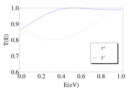
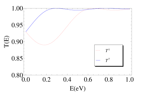
Figure 2: (Color online) Incoherent electron scattering. The electron flux moves from the left to the right planar piece through the ripple. Transmission probability $T$ as a function of the incoming electron energy : for electron with spin down (dotted line) and spin up (solid line). The sample length is $L_{0}=5\mu m$; the angle $\phi=3\pi/4$; (a) the ripple radius $R=10$Å, the ripple density $n=200\mu m^{-1}$; (b) the ripple radius $R=18$Å, the ripple density $n=100\mu m^{-1}$.

We recall that the ripples are an inherent feature of graphene. It appears that the electron reflection caused by the spin-orbital coupling, induced by the ripple curvature, is the important factor. Indeed, it determines spin dependent mean free path in the graphene sheet, which is naturally corrugated.

V Transmission across N ripples

V.1 Analytical results

The ability of the modern technology to create periodic rippled graphene structures (mentioned in Introduction) raises the question as to how the electron transport would be affected by N periodically distributed ripples. In this section we discuss the electron scattering in the graphene based superlattice. Each element of the periodic chain consists of the the ripple connected to the flat graphene piece (see Fig.1). The element includes the regions II and III. There are various approaches that allow to treat analytically this problem (e.g. Gom ). Our approach is based on the transfer matrix method, similar in spirit to the one discussed in Ref.cvet . And below we follow it to obtain our analytical results.

Let us consider the electron beam with the spin up, which is moving from the left to the right side of the superlattice. Using the continuity conditions on the boundaries, we obtain the equations for the transmission and corresponding reflection probabilities through the block of $N$ ripples in the form

$$\left(\begin{array}[]{c}1\\ r(L)^{\uparrow}_{\downarrow}\end{array}\right)=\left(\begin{array}[]{cc}A_{11}&A_{12}\\ A_{21}&A_{22}\end{array}\right)^{N}\left(\begin{array}[]{c}t(L)^{\uparrow}_{\uparrow}\\ 0\end{array}\right)\,,$$ (28)

$$A_{11}=e^{-i\Omega_{-}}\left(\cos m_{-}\phi-i\frac{A_{-}^{2}+1}{2A_{-}}\sin m_{-}\phi\right)=A_{22}^{*}\,,$$ (29)

$$A_{12}=-ie^{-i\Omega_{-}}\frac{A_{-}^{2}-1}{2A_{-}}\sin m_{-}\phi=A_{21}^{*}\,,$$ (30)

where $\Omega_{-}=kL_{1}-\phi/2$. Taking into account that there is the unitary transformation $U$ which diagonalizes the matrix A, i.e.,

$$U^{-1}AU=\left(\begin{array}[]{cc}\lambda_{1}&0\\ 0&\lambda_{2}\end{array}\right)\,,$$ (31)

we can introduce the following notations

$$\left(\begin{array}[]{cc}A_{11}&A_{12}\\ A_{21}&A_{22}\end{array}\right)^{N}=\left(\begin{array}[]{cc}N_{11}&N_{12}\\ N_{21}&N_{22}\end{array}\right)$$ (32)

with the following elements:

$$N_{11}=\frac{A_{11}[(\lambda_{1}^{\sigma})^{N}-(\lambda_{2}^{\sigma})^{N}]+(\lambda_{2}^{\sigma})^{N-1}-(\lambda_{1}^{\sigma})^{N-1}}{\lambda_{1}^{\sigma}-\lambda_{2}^{\sigma}}=N_{22}^{*}\,,$$ (33)

$$N_{12}=A_{12}A_{N}^{\sigma}=N_{21}^{*}\,,\quad A_{N}^{\sigma}=\frac{(\lambda_{2}^{\sigma})^{N}-(\lambda_{1}^{\sigma})^{N}}{\lambda_{2}^{\sigma}-\lambda_{1}^{\sigma}}\,,\quad\sigma=-\,.$$ (34)

This trick determines the eigenvalues

$$\lambda_{1,2}^{(-)}=c\pm\sqrt{c^{2}-1}\,,\quad c=(A_{11}+A_{22})/2=$$ (35)

$$=\cos\Omega_{-}\cos m_{-}\phi-\frac{A_{-}^{2}+1}{2A_{-}}\sin m_{-}\phi\sin\Omega_{-}\,.$$ (36)

Using the result $|N_{11}|^{2}-|N_{12}|^{2}=1$, we obtain

$$T^{\uparrow}=|t(L)^{\uparrow}_{\uparrow}|^{2}=\frac{1}{1+[z_{\sigma}(\phi)A_{N}^{\sigma}]^{2}}\,,\quad\sigma=-\,.$$ (37)

Following the same steps [see Eqs.(28)-(34)] for the electrons with the spin down, we obtain

$$T^{\downarrow}=|t(L)^{\downarrow}_{\downarrow}|^{2}=\frac{1}{1+[z_{\sigma}(\phi)A_{N}^{\sigma}]^{2}}\,,\quad\sigma=+\,.$$ (38)

where

$$\lambda_{1,2}^{(+)}=c\pm\sqrt{c^{2}-1}\,,$$ (39)

$$c=\cos\Omega_{+}\cos m_{+}\phi-\frac{A_{+}^{2}+1}{2A_{+}}\sin m_{+}\phi\sin\Omega_{+}\,,$$ (40)

and $\Omega_{+}=kL_{1}+\phi/2$. We also have $|r(L)^{\uparrow}_{\downarrow}|^{2}=1-|t(L)^{\uparrow}_{\uparrow}|^{2}$, $|r(L)^{\downarrow}_{\uparrow}|^{2}=1-|t(L)^{\downarrow}_{\downarrow}|^{2}$. The reflection probability without the spin-flip $|r(L)_{\alpha}^{\alpha}|^{2}=0$, as well as the transmission probability with the spin-flip $|t(L)_{\alpha}^{\beta}|^{2}=0$.

For the electron flow, moving from the right to the left side of the superlattice, we have the following relations:

$$|t(R)_{\alpha}^{\alpha}|^{2}=|t(L)_{\beta}^{\beta}|^{2}\,,$$ (41)

$$|r(R)_{\alpha}^{\beta}|^{2}=|r(L)_{\beta}^{\alpha}|^{2}\,.$$ (42)

All these results are fulfilled for the conducting band $(E>0)$. For the valence electrons $(E<0)$, the channels, through which the electron transfer occurs, are inversed with respect to those of the conductance band. In particular, the transmission probability $|t(L)^{\uparrow}_{\uparrow}|^{2}$ is determined by Eq.(38), while the transmission probability $|t(L)^{\downarrow}_{\downarrow}|^{2}$ is determined by Eq.(37) for $E<0$.

V.2 Numerical results

From the above analysis of the single ripple it follows, that in some energy interval the transport for the ballistic electrons with one spin polarization is more transparent than for those with the opposite spin polarization. To gain a better insight into the effect of the superlattice on the electron transport, we investigate numerically its dependence on: i) the number N of the ripples; ii)the radius of the ripple; iii)the angle of the ripple; iii)the distance between ripples.

For the sake of illustration, we assume that electrons move from the left to the right side of the superlattice. We observe that the transmission of electrons with the spin down is suppressed strongly in contrast to the one for the electrons with the spin up at the energy interval $0<E<0.2$ eV. The larger the number of ripples (with the same radius, angle, and the distance between ripples), the stronger the suppressing effect [compare Figs.3(a),(b)]. Thus, the number of ripples enables to us to control the suppression degree of the electron transmission with the spin down in the energy interval $0<E<0.2$ eV.

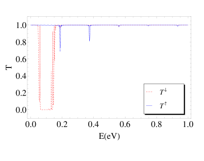
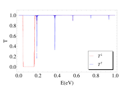
Figure 3: (Color online) The transmission probability $T$ across the superlattice as a function of the incoming electron energy for: (a) $N=40$; (b)$N=100$. The following paramenters are used: $\phi=3\pi/4$, the ripple radius $R=18$Å, the distance between the neighbouring ripples $L_{1}=65$Å.

Note, that the increasing number of ripples in the superlattice gives rise to the periodic suppression of the transmission with the spin up as well. This result can be understood as the quantum interference of the two phase factors, that are brought about by the ripple ($e^{im\phi}$) and the flat graphene piece ($e^{ikL_{1}}$). Indeed, the wave, incoming from the left boundary of the superlattice, defines a transmission coefficient $t_{l}(N^{\prime})e^{i(kL_{1}+m\phi)}$ that depends on the number $(N^{\prime})$ of the elementary units from the left boundary of the superlattice with N units $(N>N^{\prime})$. On the other hand, we have the additional contribution that is defined by the reflected wave (the reflected electron flow from the amount of ripples located on the right side of the superlattice) from the right boundary, and it has the form $t_{r}(N^{\prime}+1)e^{-i(kL_{1}+m\phi)}$ The total transmission probability from the left to the right side is determined by the formula $|t|^{2}=|t_{l}(N^{\prime})e^{i(kL_{1}+m\phi)}+t_{r}(N^{\prime}+1)e^{-i(kL_{1}+m\phi)}|^{2}=|t_{l}(N^{\prime})e^{i2(kL_{1}+m\phi)}+t_{r}(N^{\prime}+1)|^{2}$. The minimum of the probability can be expressed in the form

$$2[m_{\pm}(E)\phi+kL_{1}]=\pi(2n+1)\,,\quad n=0,1,2,\dots$$ (43)

By means of Eqs.(5,13), we arrive to the condition

$$\left(\frac{R\phi}{\gamma}\sqrt{(E-s\lambda_{x})^{2}-\lambda_{y}^{2}}+\frac{E}{\gamma}L_{1}\right)=\pi(n+1/2)\ ,\ s=\pm\,,$$ (44)

which yields

$$E\left(R\phi\sqrt{(1-s\lambda_{x}/E)^{2}-(\lambda_{y}/E)^{2}}+L_{1}\right)=\gamma\pi(n+1/2)\,.$$ (45)

At the considered energies the following condition holds: $E\gg\lambda_{x},\lambda_{y}$. It leads us immediately to the quantization condition for the energy, when the suppression takes place:

$$E_{n}\approx\frac{\gamma\pi}{R\phi+L_{1}}(n+1/2)\,,\quad n=0,1,2,\dots$$ (46)

Consequently, we find that the suppression occurs with the energy step

$$\Delta E=E_{n+1}-E_{n}=\frac{\gamma\pi}{R\phi+L_{1}}$$ (47)

as a function of the ripple radius $R$, the angle $\phi$, and the distance $L_{1}$.

This simple analysis confirms that the numerical results for the transmission minima do not depend on the electron spin polarization at large enough energies $E$ of the incoming electrons. On the other hand, when the energy $E\sim\lambda_{x}$, the term $s\lambda_{x}/E$ [see Eq.(45)] affects the transmission. In this case, there is a strong dependance of the transmission coefficient on the spin polarization as is demonstrated by the numerical computations.

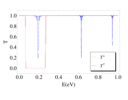
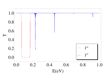
Figure 4: (Color online) The transmission probability $T$ across the superlattice as a function of the incoming electron energy for: (a) $R=8$ Å; (b)$R=18$ Å. The following parameters are used: the number of ripples $N=100$, $\phi=3\pi/4$, the distance between the neighbouring ripples $L_{1}=45$Å.

Keeping in mind, that all observed effects exhibit themselves at large number of ripples, we observe similar pattern (compare Fig.3, 4) for the transmission as a function of the incoming electron energy and the ripple radius. Note, however, that the decrease of the ripple radius increases the suppression of the transmission of the electrons with the spin down. The smaller the ripple radius, the larger the filtering effect in the energy interval $0.05<E<0.3$ eV. This fact is due to the inverse dependence of the parameters $\lambda_{x}$ and $\lambda_{y}$ on the radius [see Eq.(10)], that are responsible for the spin-orbit effect in the corrugated structure. The observed periodicity confirms remarkable well the validity of Eq.(47), that describes the suppression effect for the ballistic electrons.

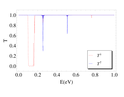
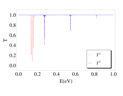
Figure 5: (Color online) The transmission probability $T$ across the superlattice as a function of the incoming electron energy for: (a)$\phi=3\pi/5$; (b)$\phi=\pi/2$. The following parameters are used: the number of ripples $N=100$; the ripple radius $R=18$ Å; the distance between the neighbouring ripples $L_{1}=45$Å.

Another variable, that affects the transmission phenomenon, is the ripple angle. It seems that the decrease of the ripple angle affects strongly the transmission phenomenon discussed above. With the increase of the ripple angle at the fixed radius (compare Figs.4b,5) the filtering effect becomes more pronounced. It appears that the smoother ripple curvature (the larger is the angle, the larger the arc length $L_{2}\approx R\phi$), the larger the filtering effects. Again, Eq.(47) describes remarkably well the periodicity of the suppressing.

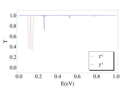
Figure 6: (Color online) The transmission probability $T$ across the superlattice as a function of the incoming electron energy for the distance between the neighbouring ripples: (a)$L_{1}=35$ Å; (b)$L_{1}=65$Å. The following parameters are used: the number of ripples $N=40$; $\phi=3\pi/4$; the ripple radius $R=18$ Å.

And finally, the effect of the distance between the neighbouring ripples yields the filtering effect in the energy interval $0.05<E<0.15$ eV (see Fiq.6). It seems the sparse rippled systems suppress the filtering effect. Indeed, in this case there is a tendency to the limit of the flat graphene where the filtering effect does not exist at all.

VI Summary

The coupling between the geometry and electron propagation in graphene sheet provides novel interesting phenomena. The nonzero curvature of the corrugated graphene region enhances the relatively weak spin-orbit interaction of the carbon atom. As a result of this interplay, we found the spin dependent electron transmission through the corrugated graphene system. Two cases of the ripple arrangement are investigating. In the first case, the interference between successive scattering events is neglecting, i.e., scattering events are treated as independent. This case can be interpreted as a natural graphene system with the disorder in the ripples positions. The transport of electrons across such a system is characterizing by the mean free path, that, in our case, is the spin dependent. In the second case, it is assumed that there is a possibility to create a periodically repeated structure of the rippled pattern in the graphene sheet. There exist the energy regions, transparent for electrons with the one spin polarization, while electrons with the opposite spin polarization are fully reflected. The situation becomes inverse, once we change the flow direction through our superlattice. The effect can be enhanced with the increasing of number elements in our superlattice. On the other hand, we can control the energy windows by altering the ripple characteristics: the radius, the angle, the length of the flat region between ripples. We found that the smaller the ripple radius, the larger the filtering effect at $N>>1$. The smoothness of the ripple can also support this effect. In our opinion, the corrugations are most possible sources of scattering phenomenon in graphene. The presence of the ripples can be the major reason that explains the finite the mean free path of the electrons in graphene, which can depend of the spin polarization. And corrugations, that can be controlled externally, could open a new avenue in nanoelectronics based on graphene based physics.

References

• (1) B. VasiΔ‡, A. Zurutuza and R. GajiΔ‡, Carbon, 102 (2016), 304
• (2) M.M.M. Alyobi, C.J. Barnett, P. Rees and R.J. Cobley, Carbon, 143 (2019), 762
• (3) G-X Ni et al., ACS Nano, 6 (2012), 1158
• (4) F. de Juan, A. Cortijo and M.A.H. Vozmediano, Phys. Rev. B, 76 (2007), 165409
• (5) T.Β Ando, J.Phys.Soc.Jpn., 69 (2000), 1757
• (6) E.A. Laird et al., Rev.Mod.Phys., 87 (2015), 703
• (7) M. Katsnelson and A.Geim, Philos. Trans. R. Soc. A, 366 (2008), 195
• (8) F. Guinea, M.I. Katsnelson and M.A.H. Vozmediano, Phys. Rev. B, 77 (2008), 075422
• (9) M. Pudlak and R.G. Nazmitdinov, J. Phys.: Condens. Matter, 31 (2019), 495301
• (10) K.N. Pichugin, M. Pudlak and R.G. Nazmitdinov, Eur. Phys. J. B, 87 (2014), 124
• (11) M. Pudlak, K.N. Pichugin and R.G. Nazmitdinov, Phys. Rev. B, 92 ( 2015), 205432
• (12) L.E.F. Foa Torres, S. Roche and J.-C. Charlier, Introduction to Graphene-Based Nanomaterials, Cambridge University Press, New York, 2014.
• (13) M.I. Katsnelson, GRAPHENE: Carbon in Two Dimensions, Cambridge University Press, Cambridge, 2012.
• (14) M. Lundstrom, Fundamentals of carrier transport, Cambridge University Press, Cambridge, 2000.
• (15) B.J.GΓ³mez, C.E.Repetto, C.R.Stia and R.Welti, Eur.J. Phys., 36 (2015), 055034
• (16) M. CveticΜ† and L. PicΜ†man, J.Phys. A: Math. Gen., 14 (1981), 379