ONETEP + TOSCAM: uniting dynamical mean field theory and linear-scaling density functional theory

Abstract

We introduce the unification of dynamical mean field theory (DMFT) and linear-scaling density functional theory (DFT), as recently implemented in ONETEP, a linear-scaling DFT package, and TOSCAM, a DMFT toolbox. This code can account for strongly correlated electronic behavior while simultaneously including the effects of the environment, making it ideally suited for studying complex and heterogeneous systems that contain transition metals and lanthanides, such as metalloproteins. We systematically introduce the necessary formalism, which must account for the non-orthogonal basis set used by ONETEP. In order to demonstrate the capabilities of this code, we apply it to carbon monoxide-ligated iron porphyrin and explore the distinctly quantum-mechanical character of the iron $3d$ electrons during the process of photodissociation.

École polytechnique fédérale de Lausanne] Theory and Simulation of Materials (THEOS), École Polytechnique Fédérale de Lausanne, 1015 Lausanne, Switzerland Newcastle University] School of Natural and Environmental Sciences, Newcastle University, Newcastle upon Tyne NE1 7RU, United Kingdom University of Warwick]Department of Physics, University of Warwick, Coventry CV4 7AL, United Kingdom University of Cambridge] Theory of Condensed Matter, Cavendish Laboratory, University of Cambridge, 19 JJ Thomson Ave, Cambridge CB3 0HE, United Kingdom King’s College London] Theory and Simulation of Condensed Matter, King’s College London, The Strand, London WC2R 2LS, United Kingdom

1 Introduction

In the last few decades, density functional theory (DFT) has established itself as a key method in computational materials science ^{1, 2, 3, 4}. Facilitated by exponentially increasing computing power, modern DFT codes are capable of routinely calculating the electronic structure of hundreds of atoms, opening the door to quantum-mechanical modeling of a vast landscape of systems of considerable scientific interest.

The range of computationally accessible systems has broadened even further with the advent of linear-scaling DFT codes (that is, codes whose computational cost scales linearly with the number of atoms in the system, rather than the cubic scaling of traditional methods). ONETEP^{5, 6} is one such code, notable for its equivalence to plane-wave approaches due to the in situ optimization of its basis (a set of local Wannier-like orbitals). Its ability to routinely perform DFT calculations on systems containing thousands of atoms allows more detailed study of nanostructures^{7, 8}, defects^{9, 10}, and biological systems^{11, 12, 13, 14}.

That said, DFT is not without its shortcomings. Many of these stem from its approximate treatment of exchange and correlation via an exchange-correlation (XC) functional. These shortcomings become especially evident in “strongly-correlated” systems, which typically contain transition element or rare-earth atoms whose $3d$- or $4f$-electron shells are partially filled. Electrons in these shells are in especially close proximity with one another, and their interaction is too pronounced to be adequately described by DFT, which can provide even qualitatively incorrect descriptions of the electronic structure. For example, DFT often yields magnetic moments inconsistent with experiment,¹⁵ predicting some insulators to be metallic,^{16, 17} and yielding equilibrium volumes dramatically different to experiment.¹⁸ DFT also fails to capture important dynamic properties that are enhanced by strong correlation, such as satellite peaks in photoemission spectra.^{19, 20}

These cases motivate the need for more accurate theories. One such approach is dynamical mean field theory (DMFT),^{21, 22, 23, 24, 25} a Green’s function method that maps the lattice electron problem onto a single-impurity Anderson model with a self-consistency condition. Local quantum fluctuations are fully taken into account, allowing DMFT to capture complex electronic behavior such as the intermediate three-peak states of the Mott transition, the transfer of spectral weight, and the finite lifetime of excitations²². Furthermore, it is possible to embed DMFT within a DFT framework, whereby only atoms with strongly-correlated electrons are treated at the DMFT level, while the rest of the system can be treated at the DFT level.¹⁷ This is critical, as DMFT alone is prohibitively expensive for studying most realistic computational models.

In the past decade, numerous codes have been written to add DMFT functionality to existing DFT packages. These include EDMFTF^{26, 27} and DFTTools²⁸ on top of Wien2K²⁹, EDMFTF²⁷ on top of VASP ^{30, 31, 32}, DCore³³ on top of Quantum Espresso ³⁴ and OpenMX^{35, 36}, TOSCAM³⁷ on top of CASTEP^{38, 39}, Amulet⁴⁰ on top of Quantum Espresso ³⁴ and Elk ⁴¹, and ComDMFT⁴² on top of FlapwMBPT^{43, 44}. Many of these make use of stand-alone libraries such as TRIQS⁴⁵, ALPS⁴⁶, iQIST ⁴⁷, or W2dynamics⁴⁸. This paper introduces the implementation of TOSCAM (A TOolbox for Strongly Correlated Approaches to Molecules) on top of ONETEP, a linear-scaling DFT code. In contrast to the packages mentioned above, this approach uniquely enables us to perform DMFT calculations on large and aperiodic systems such as nanoparticles and metalloproteins.

This code has already seen success: it has been used to explain the insulating $M_{1}$ phase of vanadium dioxide,⁴⁹ to demonstrate the importance of Hund’s coupling in the binding energetics of myoglobin,^{50, 51} and to reveal the super-exchange mechanism in the di-Cu oxo-bridge of hemocyanin and tyrosinase.⁵². But until now it has not been available to the scientific community at large. The DMFT module in ONETEP has been included in version 5.0, and TOSCAM is being released at <github link to accompany publication>. This paper presents an overview of this methodology, its implementation, and an example of its application.

2 Theory

2.1 The ONETEP framework

In the ONETEP implementation of linear-scaling DFT, we work with the single-particle density-matrix:

$$\rho(\mathbf{r},\mathbf{r}^{\prime})=\sum_{\alpha,\beta}\phi_{\alpha}(\mathrm{r})K^{\alpha\beta}\phi_{\beta}(\mathrm{r}^{\prime}),$$ (1)

where $\{\phi_{\alpha}\}$ are a set of localized non-orthogonal generalized Wannier functions (NGWFs) and $K^{\alpha\beta}$ is the density kernel. These orbitals are variationally optimized in situ during the energy-minimization carried out as part of the DFT calculation.⁵³. For the purposes of this optimization, the NGWFs are in turn expanded in terms of a systematic basis of psinc functions⁵⁴ — systematic, in the sense that the size of this basis is determined solely by a scalar parameter (a plane-wave kinetic energy cutoff determining the grid spacing) that can be increased until convergence is reached. In this scheme, a DFT calculation does not involve cyclically calculating the Kohn-Sham density and potential, but instead involves the direct minimization of the DFT energy with respect to both the density kernel and the NGWF expansion coefficients (Figure 1). Due to the fact that the NGWFs are localized, the associated matrix algebra is sparse. Meanwhile, because the NGWFs are optimized in situ, the calculations are not prone to basis set incompleteness or superposition error⁵⁵, while at the same time permitting a relatively small number of basis functions.⁵³

Figure 1: Process by which ONETEP finds a self-consistent ground-state solution for $K^{\alpha\beta}$ and $\{\phi_{\alpha}\}$.

A fully converged energy minimization yields the Kohn-Sham Hamiltonian $H_{\alpha\beta}$ in the NGWF representation, and from this, related properties such as orbital energies, electronic and spin densities, densities of states etc can be obtained. For many systems this will provide an adequate description of their electronic structure. However, in cases where we have strong electronic correlation, this Hamiltonian must be improved upon. This is the job of dynamical mean field theory.

A DMFT calculation involves the self-consistent calculation of the Green’s function ${G}^{\alpha\beta}(\omega)$ ($\omega$ here may be $\omega+i\eta$ or $i\omega_{n}$ if operating in the finite-temperature Matsubara representation) and the self-energy ${\Sigma}_{\alpha\beta}$, which are related via

$$G^{\alpha\beta}(\omega)={\left[(\omega+\mu)S-H-\Sigma(\omega)\right]_{\alpha\beta}}^{-1}$$ (2)

where $\mu$ is the chemical potential (fixed at the mid-point of the energies of the highest occupied and lowest unoccupied KS orbitals), and ${S}_{\alpha\beta}$ is the NGWF overlap matrix (that is, ${S}_{\alpha\beta}=\langle\phi_{\alpha}|\phi_{\beta}\rangle$), which is non-diagonal.

Treating most physical systems at the DMFT level would usually be prohibitively expensive. The DFT + DMFT scheme takes advantage of the fact that strong electronic correlation is often confined to identifiable localized subspaces (for instance, the $3d$ orbitals of a transition metal atom), with the remainder of the system having a delocalized, free-electron character. In such systems, the correlated subspaces can be treated at the DMFT level, while DFT alone should be sufficient everywhere else.

Correlated subspaces are typically defined via a set of local, fixed, atom-centered, spin-independent, and orthogonal orbitals $\{\tilde{\varphi}^{I}_{m}\}$. (Here, $I$ is the atom index and $m$ is an orbital index.) In ONETEP, these are defined using pseudoatomic orbitals $\{\varphi^{I}_{m}\}$, the Kohn-Sham solutions to the isolated pseudopotential of the correlated atom.^{56, 57, 58} The two are related via $|\tilde{\varphi}^{I}_{m}\rangle=|\phi_{\alpha}\rangle\langle\phi^{\alpha}|\varphi^{I}_{m}\rangle$. (Note that the pseudoatomic orbitals do not necessarily reside in the subspace spanned by the NGWFs.)

2.2 The Anderson impurity model

Figure 2: Schematic diagram of an Anderson impurity model, showing the impurity sites (orange squares), bath sites (purple circles) and the interaction parameters.

In order to efficiently find a self-consistent solution to equation 2, DMFT relies on mapping correlated subspaces to auxiliary Anderson impurity models (AIMs). The AIM is a simplified Hamiltonian that describes the interaction of a number of sites (known as impurity sites) with a bath of additional electronic levels:

$$\hat{H}=\underbrace{\sum_{ij\sigma}(\varepsilon_{ij}-\mu)\hat{c}^{\dagger}_{i\sigma}\hat{c}_{j\sigma}}_{\hat{H}_{\text{bath}}}+\underbrace{\sum_{im\sigma}\left(V_{mi}\hat{f}^{\dagger}_{m\sigma}\hat{c}_{i\sigma}+h.c.\right)}_{\hat{H}_{\text{mix}}}+\underbrace{\sum_{mm^{\prime}\sigma}(t_{mm^{\prime}}-\mu)\hat{f}^{\dagger}_{m\sigma}\hat{f}_{m^{\prime}\sigma}+\hat{H}_{U}}_{\hat{H}_{\text{loc}}}$$ (3)

where $\hat{H}_{\text{bath}}$ describes the non-correlated behavior of the bath (parameterized by the hopping matrix $\varepsilon_{ij}$), $\hat{H}_{\text{loc}}$ the impurity (parameterized by the impurity hopping $t_{mm^{\prime}}$ and the interaction Hamiltonian $\hat{H}_{U}$), and $\hat{H}_{\text{mix}}$ the coupling between the two (parameterized by $V_{mi}$). This Hamiltonian is depicted pictorially in Fig. 2. The bath and impurity sites have a shared chemical potential $\mu$, and $\hat{c}$/$\hat{f}$ are the annihilation operators for the bath/impurity. The convention throughout will be that Greek indices correspond to NGWFs, $m$ and $m^{\prime}$ to Hubbard subspaces and their corresponding impurity sites, and Latin indices to bath sites. $\sigma$ is the spin index.

The non-interacting Anderson model (i.e. $H_{U}=0$) has the Green’s function

$$G^{0}_{\text{tot}}(\omega)=\frac{1}{\omega+\mu-T}$$ (4)

where the full hopping matrix is of the block matrix form

$$T=\begin{pmatrix}t&V\\ V^{\dagger}&\varepsilon\\ \end{pmatrix}.$$ (5)

It follows that the (non-interacting) impurity Green’s function — that is, the top-left-hand block of $G^{0}_{\mathrm{tot}}(\omega)$ — simplifies to

$${{G}_{\text{imp}}^{0}}(\omega)^{-1}=\omega+\mu-t-\Delta_{\text{imp}}(\omega),$$ (6)

where

$${\Delta_{\text{imp}}}_{mm^{\prime}}(\omega)=V_{mi}\left(\frac{1}{\omega+\mu-{\varepsilon}}\right)_{ij}V^{{\dagger}}_{jm^{\prime}}$$

is the so-called impurity hybridization function. This quantity is of particular importance because it encapsulates all of the contributions of the bath sites to the physics of the impurity sites; the AIM impurity Green’s function is given by

$${G}_{\text{imp}}(\omega)^{-1}={G}_{\text{imp}}^{0}(\omega)^{-1}-{\Sigma}(\omega)=\omega+\mu-t-{\Delta}_{\text{imp}}(\omega)-{\Sigma}_{\mathrm{imp}}(\omega).$$ (7)

2.3 A DMFT calculation

This subsection will walk through the steps in a standard DMFT calculation as performed in TOSCAM + ONETEP. It is important to note that DMFT typically invokes a mean field approximation across multiple correlated sites (hence dynamical “mean field” theory), an approach that only becomes exact in the limit of infinite coordination (or equivalently, dimensions). This is not the case in our following real-space approach, where correlated sites are treated as a (possibly multi-site) AIM.

2.3.1 Mapping physical systems to an impurity model

DFT + DMFT utilizes an AIM as an auxiliary system: the AIM parameters $\{V_{mi}\}$, $\{\varepsilon_{ij}\}$, and $\{t_{mm^{\prime}}\}$ are chosen such that the resulting model Hamiltonian reproduces the physics of the real system as closely as possible. This mapping proceeds as follows. Firstly, the Kohn-Sham Hamiltonian, an estimate of the system self-energy (zero is a reasonable starting point), and a total Green’s function (obtained via equation 2) are each projected onto the correlated subspaces. For instance, the local Green’s function is given by

$${{\tilde{G}}}^{I}_{mm^{\prime}}(\omega)={W}^{I}_{m\alpha}{G}^{\alpha\beta}(\omega)(W^{I})^{\dagger}_{\beta m^{\prime}}$$ (8)

where ${W}^{I}_{m\alpha}=\langle\varphi_{m}^{I}|\phi_{\alpha}\rangle$ is the overlap of the NGWFs and the Hubbard projectors. In a similar manner one can obtain the projected self energy $\tilde{\Sigma}^{I}(\omega)$ and the projected Kohn-Sham Hamiltonian $\tilde{H}^{I}$.

We can determine the appropriate impurity hopping parameters $t_{mm^{\prime}}$ for the AIM by comparing the AIM impurity Green’s function $G_{\text{imp}}(\omega)$ and the local Green’s function $G^{I}_{mm^{\prime}}(\omega)$: if these are to match in the high=frequency limit to order $\mathcal{O}(1/\omega^{2})$ then it follows that $t=\tilde{O}^{I}W^{I}S^{-1}HS^{-1}W^{I{\dagger}}\tilde{O}^{I}$, where $\tilde{O}^{I}=(W^{I}S^{-1}W^{I{\dagger}})^{-1}$ is the overlap matrix of the projectors ${\tilde{\varphi}_{m}}$. Meanwhile, in order to define $\{V_{mi}\}$ and $\{\varepsilon_{ij}\}$, we define the local hybridization function for our physical system

$$\tilde{\Delta}^{I}(\omega)=(\omega+\mu)\tilde{O}^{I}-(\tilde{G}^{I})^{-1}(\omega)-\tilde{\Sigma}^{I}(\omega)-\tilde{H}^{I}$$ (9)

which is analogous to the definition of the impurity hybridization function (equation 7). We choose the impurity model bath parameters such that the AIM hybridization function matches this local hybridization function as closely as possible. This is done by minimizing the distance function

$$d(V,\varepsilon)=\sum_{\omega<\omega_{c}}\frac{1}{\omega^{\gamma}}\left|\Delta_{\text{imp}}(\omega)-\tilde{\Delta}^{I}(\omega)\right|^{2}$$ (10)

using a conjugate gradient (CG), Broyden-Fletcher-Goldfarb-Shanno (BFGS), or similar minimization algorithm. Here, $\omega_{c}$ is a cutoff frequency and $\gamma$ is a user-specified parameter that can allow for preferential weighting of agreement at low frequencies.

In order to complete the construction of the auxiliary AIM Hamiltonian we choose $H_{U}$ to be of the Slater-Kanamori form^{59, 60}

$$\hat{H}_{U}=U\sum_{m}\hat{n}_{m\uparrow}\hat{n}_{m\downarrow}+\left(U^{\prime}-\frac{J}{2}\right)\sum_{m>m^{\prime}}\hat{n}_{m}\hat{n}_{m^{\prime}}$$

$$-J\sum_{m>m^{\prime}}(2\hat{\mathbf{S}}_{m}\hat{\mathbf{S}}_{m^{\prime}}+\hat{f}^{\dagger}_{m\uparrow}\hat{f}^{\dagger}_{m\downarrow}\hat{f}_{m^{\prime}\uparrow}\hat{f}_{m^{\prime}\downarrow}).$$ (11)

This Hamiltonian is well-suited to capturing multiplet properties of low energy states.⁶¹ Its first term describes intra-orbital Coulomb repulsion. The second describes the inter-orbital repulsion, with $U^{\prime}=U-2J$ further renormalized by the Hund’s coupling to ensure the rotational invariance of the Hamiltonian. The third and final term captures the Hund’s exchange coupling; $\hat{\mathbf{S}}_{m}$ is the spin of orbital $m$, given by $(\hat{\mathbf{S}}_{m})_{i}=\frac{1}{2}\sum_{\sigma\sigma^{\prime}}\hat{f}^{\dagger}_{m\sigma}(\mathbf{s}_{i})_{\sigma\sigma^{\prime}}\hat{f}_{m\sigma^{\prime}}$ via the Pauli spin matrices $\{\mathbf{s}_{i}\}$. The Hubbard parameter $U$ and Hund’s coupling $J$ are user-specified parameters that in principle could be obtained via linear response ⁶² but are often chosen empirically or treated as variational parameters.

Now that we have defined $\varepsilon$, $V$, $t$, and $H_{U}$, the mapping of a real system to an auxiliary AIM is complete. In theory, this mapping can be exact: as long as $\Delta_{\text{imp}}(\omega)$ and $\tilde{\Delta}^{I}(\omega)$ match exactly, $G_{\text{imp}}(\omega)$ and $\tilde{G}^{I}(\omega)$ will also. Getting this mapping right is therefore of the utmost importance.

2.3.2 Solving the AIM

Having constructed the AIM Hamiltonian $H_{\text{AIM}}$, the next step is to calculate the Green’s function of the AIM (known as the impurity Green’s function):

$${G_{\text{imp}}}_{mm^{\prime}}(\omega) =\int_{-\infty}^{\infty}e^{i\omega t}{G_{\text{imp}}}_{mm^{\prime}}(t)\,dt$$

$$=-i\int_{0}^{\infty}e^{i\omega t}\langle{e^{i\hat{H}t}\hat{c}_{m}e^{-i\hat{H}t},\hat{c}^{\dagger}_{m^{\prime}}}\rangle\,dt$$

$$=-i\left(\left\langle\hat{c}_{m}\int_{0}^{\infty}e^{i(\omega-(\hat{H}-E_{0}))t}\,dt\,\hat{c}^{\dagger}_{m^{\prime}}\right\rangle+\left\langle\hat{c}^{\dagger}_{m^{\prime}}\int_{0}^{\infty}e^{i(\omega+(\hat{H}-E_{0}))t}\,dt\,\hat{c}_{m}\right\rangle\right)$$

$$=\left\langle\hat{c}_{m}\frac{1}{\omega-(\hat{H}-E_{0})}\hat{c}^{\dagger}_{m^{\prime}}\right\rangle+\left\langle\hat{c}^{\dagger}_{m^{\prime}}\frac{1}{\omega+(\hat{H}-E_{0})}\hat{c}_{m}\right\rangle$$ (12)

where $\langle~{}\bullet~{}\rangle$ is the thermodynamic average, which at zero temperature becomes $\langle\psi_{0}|~{}\bullet~{}|\psi_{0}\rangle$.

Resolving equation 12 is highly expensive, and becomes one of the most substantial computational barriers in a DMFT calculation. If there are $m$ bath sites and $n$ impurity orbitals, the Hilbert space of this problem scales as $4^{m+n}$. (For a system containing a single transition metal there will be five impurity orbitals — one for each $3d$ orbital — and then typically six to eight bath sites.) This is far larger than any of the other matrix inversions that we need to calculate during the DMFT loop (for instance, $G^{\alpha\beta}$ is only as large as the number of Kohn-Sham orbitals, which in turn will be of the order of the number of electrons in the physical system — typically several thousand at most). There are a number of approaches for obtaining $G_{\text{imp}}$, such as exact diagonalization (ED) and continuous time Monte Carlo algorithms. The calculations in this work employ ED via the Lanczos algorithm to evaluate equation 7, a process which is explained in detail in the Supplementary Information.

Given a solution $G_{\text{imp}}$ (obtained via ED or otherwise), the impurity self-energy can then be obtained via

$$\Sigma_{\text{imp}}(\omega)=[G^{0}_{\text{imp}}]^{-1}(\omega)-G_{\text{imp}}^{-1}(\omega)$$ (13)

where the non-interacting impurity Green’s function is given by equation 6. Note that this operation is far less expensive than equation 7 because these matrices are only $m\times m$ in size.

2.3.3 Upfolding and double-counting

Having obtained the impurity Green’s function $\Sigma_{\text{imp}}^{I}$ for each AIM, the final step is to upfold this result to the complete physical system. Since the original DFT solution already contains the influence of the Coulomb interaction to some degree, double-counting becomes an issue. A popular form of the correction is

$$E_{\mathrm{DC}}=\frac{U^{\mathrm{av}}}{2}n\left(n-1\right)-\frac{J}{2}\sum_{\sigma}n_{\sigma}(n_{\sigma}-1)$$ (14)

where $n$ is the total occupancy of the subspace, $n^{\sigma}$ is the occupancy of the subspace for the spin channel $\sigma$, and

$$U^{\mathrm{av}}=\frac{U+2(N-1)U^{\prime}}{2N-1}$$ (15)

with $N$ being the number of orbitals spanning the correlated subspace (and recall that $U^{\prime}=U-2J$).⁶¹ This double-counting is derived by attempting to subtract the DFT contributions in an average way; $U^{av}$ is the average of the intra- and inter-orbital Coulomb parameters.

The self-energy is upfolded to the NGWF basis via

$$\Sigma_{\alpha\beta}=\sum_{I}{W^{I}}^{{\dagger}}_{\alpha m}({\Sigma^{I}}^{mm^{\prime}}-E_{\mathrm{DC}}\tilde{O}^{mm^{\prime}})W^{I}_{m^{\prime}\beta}$$ (16)

— and with that, we are back where we started, having generated a new estimate of the self-energy $\Sigma_{\alpha\beta}$ for the full system.

To summarize, the scheme is as follows:

1. perform a DFT calculation to construct the system Hamiltonian

2. initialize the self-energy as $\Sigma_{\alpha\beta}(\omega)=0$

3. obtain the Green’s function for the full system (equation 2)

4. project the total Green’s function and self energy onto the $I$^th Hubbard subspace to obtain the corresponding local quantities (equation 8)

5. calculate the local hybridization function (equation 9)

6. find the bath parameters $\varepsilon_{ij}$ and $V_{mi}$ such that the AIM hybridization function (equation 2.2) matches the local hybridization function found above

7. explicitly solve the AIM Hamiltonian to obtain the impurity Green’s function (equation 12)

8. update the impurity self-interaction (equation 13)

9. upfold the self-energies from each correlated subspace to obtain the total self-interaction (equation 16)

Note that if we only have one correlated site in our system, this mapping is exact, and the local lattice Green’s function at step 9 will already match the impurity Green’s function.

This is not the case for bulk systems. There, the mean field approximation that we adopt means that the self-energy of a correlated site is also inherited by the “bath” i.e. one would typically solve a single Anderson impurity problem but then in equation 16, the index $I$ would run over all correlated sites. This means that after step 9 we must return to step 3, and repeat this loop until the local lattice and impurity Green’s functions match.

Once the calculation is converged, we can extract system properties from the Green’s function. For example, DFT+DMFT total energies can be calculated via

$$E=E_{\mathrm{DFT}}[\rho]-\sum_{i\sigma}\varepsilon_{i\sigma}+\mathrm{Tr}[H_{\mathrm{KS}}G]+\frac{1}{2}\mathrm{Tr}[\Sigma G]-E_{\mathrm{DC}}+E_{\mathrm{nuc-nuc}}$$ (17)

where the first term is the DFT energy functional, $\varepsilon_{i\sigma}$ are the Kohn-Sham eigenenergies, $H_{KS}$ is the Kohn-Sham Hamiltonian, $G$ is the full Green’s function, the fourth term is the DMFT contribution to the potential energy $\langle\hat{H}_{U}\rangle$ calculated via the Migdal-Galitskii formula, the fifth term is the double-counting correction (equation 14), and the final term is due to the interaction between atomic cores (that is, both the nuclei and the pseudized electrons).^{23, 63, 64} When calculating the DMFT potential energy contribution, we use the high-frequency expansion technique of Pourovskii et al.⁶⁵ For an example of ONETEP+TOSCAM DFT+DMFT energy calculations, see Refs.  50 and   51, where some of us presented a detailed study of heme and myoglobin binding to CO and other small molecules.

Other quantities that can be extracted from the Green’s function include the density of states and the optical absorption. One can also apply standard ONETEP analysis techniques to the electron density (such as natural bonding orbital analysis). These techniques will be demonstrated in Section 3.

2.4 Extensions

There are several possible extensions to the theory described thus far. These are not essential but often useful.

2.4.1 Enlarged AIM via cluster perturbation theory

If an AIM has too few bath sites at its disposal, it will be insufficiently flexible to fit a given local hybridization function. The brute-force approach would be to increase the number of bath sites, but in practice the number of bath sites is severely limited due to the exponential growth of Hilbert space with respect to the total number of sites (bath and impurity) of the AIM. To overcome this barrier, a secondary set of bath levels are coupled to the primary bath levels via cluster perturbation theory. By indirectly including these sites, the AIM system acquires extra flexibility without expanding the Hilbert space, resulting in a dramatic drop in the distance function. For more details, see Ref.  66.

2.4.2 Self-consistency

For a system with a single correlated site, there is no feedback from the self energy to the hybridization function, and — provided the AIM is sufficiently representative — the DMFT algorithm will converge in a single step. In this case the algorithm is not a mean-field approximation, but exact. This scheme is shown in Fig. 3(a).

However, there are a number of reasons why we may not be content with the resulting solution. Firstly, the total number of electrons in the system is related to the total retarded Green’s function via

$$N=\int d\omega\,\rho^{\alpha\beta}(\omega)S_{\alpha\beta};\qquad\rho^{\alpha\beta}(\omega)=\frac{1}{2\pi i}\left(G^{\alpha\beta}(\omega)-{G^{\alpha\beta}}^{\dagger}(\omega)\right),$$ (18)

where $\rho^{\alpha\beta}(\omega)$ is the basis-resolved DMFT density matrix. There is no reason a priori why the Green’s function, updated via the DMFT loop, should yield the same number of electrons as we started with — in fact, this is almost never the case. For this reason, charge conservation can optionally be enforced by adjusting $\mu$ so that $\int_{-\infty}^{\mu}\rho(\omega)=N$. This update is performed during each DMFT cycle, which means that our total Green’s function (now adjusted by our altered $\mu$) will not necessarily be consistent with the self energy — and consequently more than one DMFT loop will likely be required to iterate to self-consistency (Fig. 3(b)). We will refer to this as “charge-conserving” DMFT.

Finally, in the DFT formalism, the Hamiltonian is a functional of the density. It could be argued that if we are to be fully self-consistent, if ever the density changes the Hamiltonian should be updated accordingly. In this scheme, one iterates until $\Sigma$, $H$, and $\mu$ all converge (Fig. 3(c)). This we will refer to as “fully self-consistent” DMFT. We use Pulay mixing^{67, 68} to update the Hamiltonian (via the density kernel) and the self-energy. Performing this double-loop naturally makes the calculations much more expensive, but they remain feasible. This approach was taken in Refs.  65– 70, for example.

(a) single-shot

(b) charge-conserving

(c) self-consistent

Figure 3: The three DMFT schemes, in increasing order of complexity.

2.5 Practical implementation

In our implementation, ONETEP and TOSCAM are responsible for separate sections of the DMFT loop, as shown in Figure 4. As the calculation proceeds, these two programs are called in alternation, with the entire procedure being driven by an overarching script.

This splitting makes our algorithm highly amenable to parallelization: parallel TOSCAM instances can consider different correlated subspaces in isolation. That is, a system with many correlated sites is embarrassingly parallel if inter-site correlation can be neglected. By design, the AIM solver in TOSCAM is as modular as possible. This allows for it to be easily interchanged with other solvers that have been independently developed.

Figure 4: A simplified DMFT loop, demonstrating which program (ONETEP or TOSCAM) is responsible for which step.

TOSCAM is freely available; email cedric.weber@kcl.ac.uk to be given access to the git repository. Note that it is dependent on ONETEP (version 5.0 and later), which can be obtained separately (see www.onetep.com).

2.6 Scaling

One of our primary considerations is how ONETEP+TOSCAM calculations scale. As discussed already, obtaining the Green’s function of the AIM scales very poorly with the number of AIM sites. This is shown in Fig. 5a. We are not entirely in a position to dictate the number of AIM sites: a $3d$ correlated site is represented as a five-site impurity, and typically we need to include at least six bath sites to give the AIM sufficient flexibility to fit the hybridisation function.

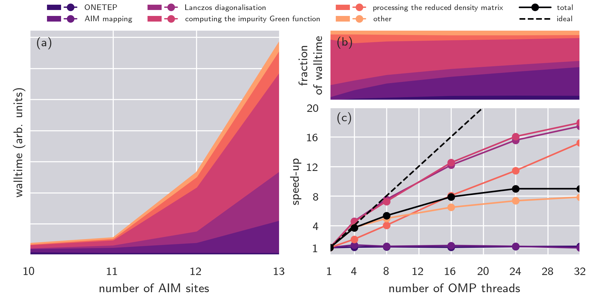
Figure 5: The scaling of ONETEP+TOSCAM for calculations on iron porphyrin (see Section 3 for details). (a) The scaling with respect to the number of AIM sites; (b) and (c) the fractional wall time and the speed-up with respect to the number of OpenMP threads. “Lanczos diagonalisation” and “computing the impurity Green’s function” are two steps involved in solving the AIM; for details refer to the Supplementary Information.

To some extent, poor scaling can be overcome by efficient parallelization. Both ONETEP and TOSCAM employ hybrid MPI and OpenMP parallelization schemes. ONETEP’s parallelization is highly optimized. Individual atoms are distributed across MPI threads, with lower-level computationally-intensive operations (including 3D FFT box operations, sparse matrix algebra operations, calculation of integrals, and Ewald summation) being further parallelized with OpenMP.⁷¹

In the implementation of TOSCAM, individual MPI tasks are responsible for individual correlated atoms. For systems where we have only one unique correlated atom, MPI becomes redundant. Meanwhile, OpenMP is deployed to speed up lower-level operations (see Fig. 5b and c).

3 Iron porphyrin

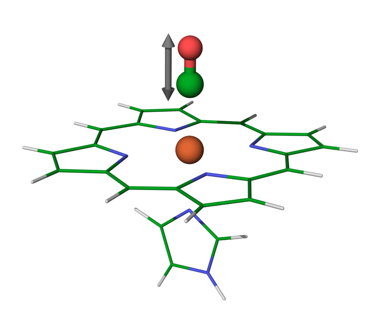
(a)

(b)

Figure 6: (a) The model complex studied in this work: iron porphyrin with axial imidazole and carbon monoxide ligands. Hydrogen, carbon, nitrogen, oxygen and iron atoms are shown in white, green, blue, red, and orange respectively. (b) Carboxymyoglobin, showing the iron binding site.⁷²

To demonstrate the use of the ONETEP+TOSCAM interface, the second half of this paper presents some calculations on an archetypal strongly-correlated system: an iron porphyrin ring with imidazole and carbon monoxide as the axial ligands (FePImCO) shown in Fig. 6a, a toy model for the full carboxymyoglobin complex (Fig. 6b). By translating the carbon monoxide molecule perpendicular to the porphyrin plane, we model the photodissociation of carboxymyoglobin. Myoglobin is one of the most ubiquitous metalloproteins. Previous studies have successfully applied DMFT in order to rationalise its binding energetics,^{50, 51} and there are unresolved questions surrounding the process of carbon monoxide photodissociation, as we shall discuss.

3.1 Computational details

All DFT calculations were performed using a modified copy of ONETEP.^{5, 73, 74, 75, 58, 76} Those modifications were subsequently included in ONETEP 5.0. All calculations used the PBE XC functional,⁷⁷ were spin-unpolarised, and had an energy cut-off of 908 eV. There were thirteen NGWFs on the iron atom, four on each carbon, nitrogen, and oxygen, and one on each hydrogen. All NGWFs had 6.6 Å cut-off radii. Open boundary conditions were achieved using a padded cell and a spherical Coulomb cut-off.⁷⁸ Scalar relativistic pseudopotentials were used, generated in-house using OPIUM,^{79, 80, 81, 82, 83, 84, 85, 86} and the Hubbard projectors were constructed from the Kohn-Sham solutions for a lone iron pseudopotential.⁵⁸

The bound structure was taken from Ref.  87, which had been optimized with the B3LYP functional. The other structures were generated by simply translating the carbon monoxide molecule in steps of 0.1Å, without subsequently performing a geometry optimization of the rest of the system. (An ideal analysis would involve a constrained geometry optimization, to account for effects such as doming.)

Both charge-conserving and self-consistent calculations were performed, using enlarged AIM Hamiltonians via the cluster perturbation theory (CPT) extension. Seven bath orbitals proved necessary for the AIM to be able to fit the hybridization function using the BFGS minimisation algorithm, and the AIM was solved using an ED Lanczos solver. Values of $U=4.0$ eV and $J=0.7$ eV were used in the AIM Hamiltonian. The DMFT calculations were deemed to have converged when (a) the chemical potential changed by less than 1 mHa, (b) the total number of electrons was within 0.01e of the target value, and (c) the occupancy of the correlated subspace changed by less than 0.01 electrons from one iteration to the next.

Example input and output files can be found on Materials Cloud.⁸⁸

3.2 The quantum-mechanical state of the 3d iron subspace

A large effort (largely in the quantum chemistry community) has been made to correctly predict the spin state of Fe(II)P with (and without) a variety of axial ligands. These range from decades-old Hartree-Fock calculations to recent FCIQMC studies.^{89, 90, 91, 92, 93, 94} FePImCO is one of the simpler cases, with a singlet state universally predicted. Meanwhile, FePIm has proven to be more of a challenge. Experiment characterises FePIm as a quintet. Semi-local DFT wrongly predicts it to be a triplet (as shown in Fig. 7). DFT + $U$ remedies this,⁹⁵ as does Hartree-Fock (HF).⁸⁹

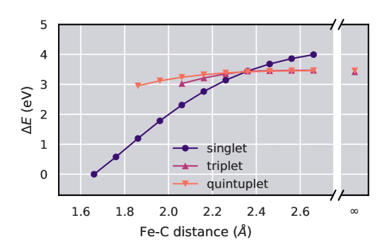
Figure 7: Spin state energies as given by DFT. For FePImCO the singlet state is correctly preferred, but for FePIm the triplet is wrongly preferred, albeit only very marginally (by 34 meV).

To start, we will examine the charge transfer that takes place during CO dissociation in the DFT + DMFT picture. The Fe atom in FePIm is formally in the 2+ state ($d^{6}$). When it binds CO, it moves closer to 1+ ($d^{7}$) due to ligand-to-metal charge transfer. This is corroborated by our DFT+DMFT calculations: the occupancy of the $3d$ subspace can be calculated via

$$n_{3d}=\frac{1}{2\pi i}\sum_{m}\int\mathrm{d}\omega\,{G_{\mathrm{imp}}}_{mm}(\omega)-{{G_{\mathrm{imp}}}_{mm}}^{\dagger}(\omega).$$ (19)

This is plotted in Fig. 8a as a function of the Fe–C distance. The unbinding is plainly visible as a sudden step in the total occupancy, at the same distance that DFT predicted the low-to-high-spin crossover (refer back to Fig. 7). The effect of DMFT is especially pronounced at large Fe-C distances, where it drives the subspace occupancy towards the expected formal $d^{6}$ configuration. (In some sense, DMFT restores the quantized nature of the electrons in the correlated subspace that is absent in DFT.)

As a means of analysing the spin state of the iron atom during the dissociation process with DMFT, we construct the reduced density matrix

$$\hat{\rho}=\sum_{i}e^{-\beta E_{i}}\mathrm{Tr}_{B}[|i\rangle\langle i|],$$ (20)

where we take the partial trace of the low-lying eigenstates of the AIM over the bath degrees of freedom, leaving a mixed density operator for the impurity alone. It is then straightforward to calculate the expectation value of $\hat{S}^{2}=\sum_{i,j}\hat{\mathbf{S}}_{i}\cdot\hat{\mathbf{S}}_{j}$ and extract the effective spin $S_{\mathrm{eff}}$ (Fig. 8b). Here we can see that at large distances we approach the quintet $S_{\mathrm{eff}}=2$. At small distances we are closer to the triplet value $S_{\mathrm{eff}}=1$. Note that this does not mean that DMFT has failed to predict that FePImCO is a singlet. Rather, this result is compatible with (but does not confirm the existence of) a singlet forming across the Fe-CO bond. By limiting ourselves to the Fe subspace we cannot directly measure such a singlet.

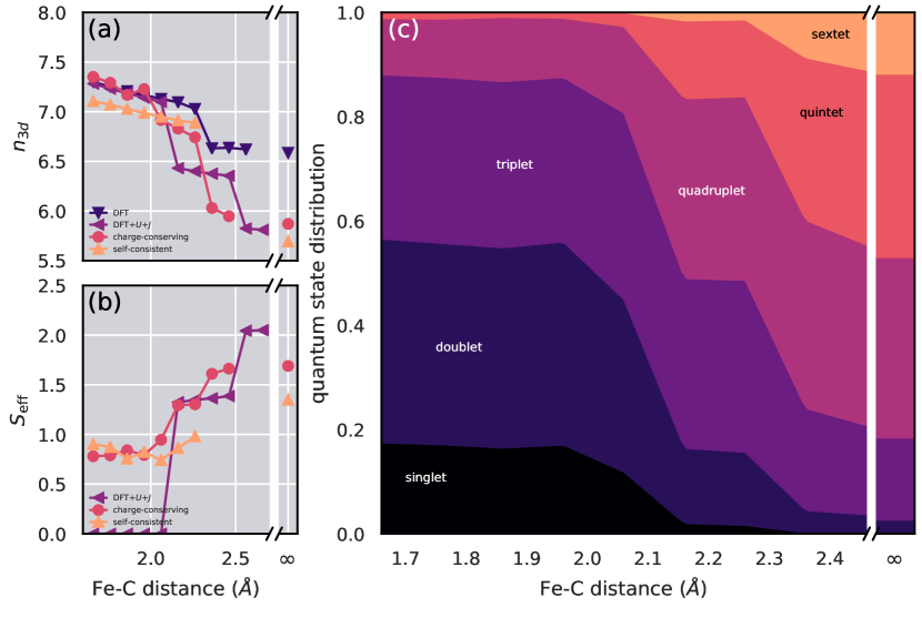
Figure 8: The electronic state of iron in FePImCO during CO dissociation. (a) The total occupancy of the Fe-$3d$ subspace as given by DFT and two different DMFT schemes. Unfortunately self-consistent DMFT calculations proved very difficult to converge beyond the low-to-high spin transition, so these results have been excluded throughout. Below this transition, the two methods qualitatively agree. (b) The effective spin $S_{\mathrm{eff}}$ of the reduced density matrix, defined via $\mathrm{Tr}[\hat{S}^{2}\hat{\rho}]=\hbar^{2}S_{\mathrm{eff}}(S_{\mathrm{eff}}+1$) for the DMFT calculations and as $S_{\mathrm{eff}}=\frac{1}{2}(n^{\uparrow}_{3d}-n^{\downarrow}_{3d})$ for the broken-symmetry DFT+$U$+$J$ calculations. (c) The decomposition of the reduced density matrix by spin state. The colours correspond to the respective weights of the different contributions; if a colour occupied all the vertical axis, it would mean that all eigenvectors of the density matrix are in that particular quantum sector.

For comparison, we also present the occupancy and spin of the $3d$ subspace as calculated by DFT+$U$+$J$, using the same $U$ and $J$ parameters as for the DFT+DMFT calculations. DFT+$U$(+$J$) is a widespread and computationally cheap correction to DFT for accounting for electronic correlation, and is equivalent to solving the DMFT impurity problem at the level of Hartree-Fock.^{96, 97, 98, 75} We note that DFT+$U$+$J$ recovers the correct quintet spin state in the dissociated limit, in line with previous DFT+$U$ studies⁹⁵, with a window where the triplet state is favored. Furthermore, the singlet state becomes unstable at a shorter Fe–C distance of around 2 Å (see Fig. 8b). This is a common feature of DFT+$U$,^{99, 100} where the corrective $+U$ potential reduces the hybridization between the correlated subspace and the ligand orbitals, thereby weakening the bond between them. Addressing this within a Hubbard model framework requires more sophisticated approaches such as inter-site terms⁹⁹ or applying corrective Hubbard potentials to ligand subspaces.¹⁰⁰ This is not a problem that DMFT suffers from.

To inspect the DMFT reduced density matrix in more detail, one can construct the spin-projector

$$\hat{P}_{S}=\sum_{s\in S}|s\rangle\langle s|$$ (21)

as the sum of the eigenstates $|s\rangle$ of the operator $\hat{S}^{2}$ with eigenvalue $S(S+1)$. This allows us to evaluate the fraction of the reduced density matrix in singlet, doublet, triplet, and higher states via $\mathrm{Tr}[\hat{P}_{S}\hat{\rho}\hat{P}_{S}]$ for $S=0$, $\frac{1}{2}$, $1$ etc. Note, however, that this approach is incompatible with the CPT extension. The CPT extension involves solving an auxiliary AIM Hamiltonian that shares the same impurity Green’s function as a larger AIM Hamiltonian, and consequently any quantities derived directly from the Green’s function will be unaffected. However, there is no such guarantee for the reduced density matrix, because the hybridization function of this auxiliary system does not necessarily match that of the physical system. To overcome this, the CPT extension was at first applied in order to obtain an approximate solution, but then removed for the final DMFT step. Typically this final step required the addition of an extra bath site so that the AIM acquired sufficient flexibility to fit the impurity hybridization function to the local hybridization function without the assistance of the CPT extension.

The decomposition of the reduced density matrix into spin sectors is displayed in Fig. 8c. It reveals a large quintet state contribution in the limit of dissociation, but also that, regardless of Fe-C distance, many different spin sectors are important. This would be missed if we only examined $S_{\mathrm{eff}}$ or only performed DFT.

Evidently, a multitude of states play an important role throughout CO-unbinding, and therefore the success of DFT + $U$ and HF in predicting the quintet ground state must be for the wrong reasons, as neither go beyond the single-determinantal picture. (Note that HF is known to overly favour high-spin states.¹⁰¹)

It should be noted that the precise details of Fig. 8 are somewhat sensitive to various simulation parameters — most notably the definition of the Hubbard projectors — but qualitatively the results are expected to hold generally.

3.3 Photodissociation

The photodissociation mechanism of carboxymyoglobin is already relatively well understood. Irradiation at 570 nm (2.18 eV) causes the excitation of electrons in the porphyrin ring into low lying singlet states with $\pi$/$\pi^{*}$ character (the so-called Q band).¹⁰² The carbon monoxide ligand then dissociates within 50 fs, as the system adiabatically crosses to a repulsive anti-back-bonding orbital.^{103, 104} There is a small (but not insignificant) predicted energy barrier of 0.08 eV between these two states, as calculated by B3LYP and TDDFT.⁸⁷ The porphyrin then undergoes the “intersystem crossing”, a complicated, multi-step process which ultimately takes the dissociated system to its high-spin ground state.

Semi-local DFT captures this process qualitatively. The energies of the lowest unoccupied KS molecular orbitals as predicted via DFT are shown in Fig. 9. The Q band is present, and the pathway from the Q band to the anti-back-bonding orbital is clearly visible via their crossing at approximately 2.3 Å (the same distance we observe the low-to-high spin crossover in Fig. 7), with an energy barrier of approximately 0.13 eV. Compared to the TDDFT/B3LYP results of Refs.  103 and 104, PBE calculations place this crossover at a much longer distance (approximately 2.3 Å compared to 2.0 Å), and predict that the energy of the anti-back-bonding orbital drops much more steeply. (Head-Gordon and co-workers noted that the very gentle decrease in the energy of the anti-back-bonding orbital as predicted by their TDDFT/B3LYP calculations is at odds with the $\sim 50$ fs timescale of photodissociation.¹⁰⁴)

Figure 9: Energies of the KS molecular orbitals, measured relative to the highest occupied orbital of the tightly-CO-bound structure.

To compare the results of DMFT to these KS eigenenergies, the analogous quantity we must extract is the DOS. The DOS is given by the trace of the many-body density matrix

$$\rho(\omega)=\sum_{\alpha,\beta}\rho^{\alpha\beta}(\omega)S_{\beta\alpha}.$$ (22)

The DMFT DOS is compared to the KS eigenenergies in Fig. 10. Qualitatively, they yield very similar results, but with DMFT (unlike DFT) we obtain the lifetime of the excitations.

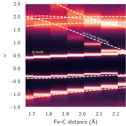
Figure 10: The DMFT DOS of FePImCO during dissociation, compared to the KS eigenenergies (white dashed lines), as given by self-consistent DMFT calculations. The DOS and eigenenergies have been aligned to match the Q band, because, being a porphyrin-ring state, it should not be significantly shifted by DMFT.

To reveal the contribution of individual atoms (or groups of atoms) towards the DMFT DOS, it can be decomposed into local densities of state (LDOSs)

$$\rho_{I}(\omega)=\sum_{\alpha\in I}\sum_{\beta}\rho^{\alpha\beta}(\omega)S_{\beta\alpha},$$ (23)

where $I$ denotes a subset of NGWFs typically belonging to atoms that are a particular element or part of a spatially distinct subsystem (e.g. all the NGWFs belonging to atoms in the porphyrin ring). One such LDOS is plotted in Fig. 11, along with isosurfaces of the spectral density at energies corresponding to the various peaks in the DOS. The Q-band $\pi/\pi^{*}$ orbitals and the Fe-CO back- and anti-back-bonding orbitals are all clearly identifiable.

Figure 11: Self-consistent DMFT density of states for carboxy-heme with a Fe-C distance of 2.06 Å. The DOS is further decomposed into contributions from the iron atom, CO molecule, imidazole ligand and porphyrin ligand. Above, isosurfaces of $\rho(\mathbf{r},\omega_{\text{peak}})$ have been plotted for each peak.

Another important quantity that can be extracted from DMFT calculations is the optical spectrum. The theoretical optical absorption spectrum can be obtained within the linear-response regime (that is, Kubo formalism) as

$$\sigma_{ij}(\omega)=\frac{2\pi}{\Omega}\int d\omega^{\prime}\frac{f(\omega^{\prime}-\omega)-f(\omega^{\prime})}{\omega}\left(\rho^{\alpha\beta}(\omega^{\prime}-\omega)\mathbf{v}^{i}_{\beta\gamma}\rho^{\gamma\delta}(\omega^{\prime})\mathbf{v}^{j}_{\delta\alpha}\right)$$ (24)

where $\Omega$ the simulation cell volume, $f(\omega)$ is the Fermi-Dirac distribution, $\rho$ is the basis-resolved spectral density, the $i$ and $j$ indices correspond to Cartesian directions, the velocity operator $\mathbf{v}$ is

$$\mathbf{v}^{j}_{\alpha\beta}=-i\langle\alpha|\nabla_{j}|\beta\rangle+i\langle\alpha|\left[\hat{V}_{nl},\mathbf{r}\right]|\beta\rangle$$ (25)

which includes the effect of non-local pseudopotentials $V_{nl}$ on the velocity operator matrix elements, and adopts the no-vertex-corrections approximation.¹⁰⁵ Optical spectra for heme are typically carried out in liquid or gas phases, and so are described by the isotropic part of the optical conductivity tensor

$$\sigma(\omega)=\frac{1}{3}\sum_{i}\sigma_{ii}(\omega).$$ (26)

The optical absorption spectra for carboxy-heme complexes as given by self-consistent DMFT are plotted in Fig. 12. These spectra are dominated by a feature at around 2 eV associated with $\pi$-$\pi^{*}$ transitions on the porphyrin ring — that is, the Q band. The double-peak structure of the Q band is successfully reproduced. (Ref.  51 found that $J>0$ is necessary to obtain this double-peak feature.) Secondary peaks appear above 3 eV corresponding to direct photoexcitation of the anti-back-bonding orbital.

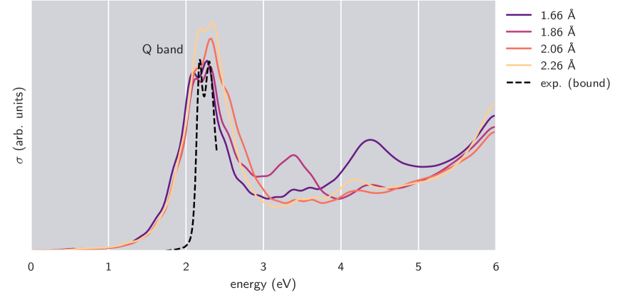
Figure 12: Optical spectra of FePImCO calculated using self-consistent DMFT, going from ligated (dark) up to the point of dissociation (light). Also pictured are the Q-band peaks from experimental spectra of carboxymyoglobin.¹⁰⁶

4 Conclusions

This paper has described how DMFT has been interfaced with linear-scaling DFT in the ONETEP+TOSCAM implementation. Crucially, for the purposes of simulating metalloproteins, this DFT + DMFT implementation does not compromise our ability to model thousands of atoms at the DFT level, opening up a new frontier for accurate simulation of complex and heterogeneous systems containing transition metals and lanthanides.

The ONETEP+TOSCAM interface will continue to be developed. In particular, work is underway to compute forces at the DFT+DMFT level (as has been achieved elsewhere^{107, 37}), a GPU implementation of the ED solver will be incorporated, as well as a CTQMC solver (which will allow us to solve substantially larger AIMs.) Note that it is straightforward to add additional solvers due to the modularity of the code.

Calculations on the photodissociation of carboxymyoglobin showcased the kinds of results one can extract from such a DFT + DMFT calculation on a metalloprotein, including some — such as the mixed quantum state of the iron $3d$ subspace and the finite lifetime of excitations — that are inaccessible via DFT. And while the calculations do not reveal any previously unknown physics, there is scope here to resolve some unanswered questions surrounding the photodissociation process. In particular, the remarkably fast rate of photodissociation ($\sim 50$ fs) is at odds with the gentle slope of the potential energy surface (discussed above) and the predicted barrier on the order of 0.1 eV (compared to the 0.028 eV zero-point energy of the Fe-C stretching mode).⁸⁷ Further study could investigate this apparent contradiction.

EBL acknowledges financial support from the Rutherford Foundation Trust and the EPSRC Centre for Doctoral Training in Computational Methods for Materials Science under grant EP/L015552/1. NDMH acknowledges the support of the EPSRC under grant EP/P02209X/1. MCP acknowledges the support of the EPSRC under grant EP/P034616/1. CW acknowledges the support of the EPSRC under grant EP/R02992X/1. The authors thank M. A. Al-Badri and M. J. Rutter for useful discussions. This work was performed using the Darwin Supercomputer of the University of Cambridge High Performance Computing Service (http://www.hpc.cam.ac.uk/), provided by Dell Inc. using Strategic Research Infrastructure Funding from the Higher Education Funding Council for England and funding from the Science and Technology Facilities Council.

The Supporting Information contains a brief description of the TOSCAM/ONETEP interface, as well as relevant links, and an introduction to the Lanczos algorithm and how it may be used to solve the Anderson impurity model.

Supplementary Material

1 Accessing the codes

ONETEP is available under academic license to all UK academics and is also part of Materials Studio (http://accelrys.com/products/datasheets/onetep.pdf). For more details see www.onetep.com.

To obtain the source code for TOSCAM, contact Cédric Weber to be granted access to the git repository. TOSCAM is distributed under the lesser GNU public license.

2 Exact Diagonalization

2.1 The standard Lanczos algorithm

The Lanczos method is an approach for obtaining the eigenvectors and eigen-energies of a Hermitian matrix $A$, without ever having to perform a full diagonalisation. Starting with some arbitrary normalised vector $|0\rangle$, we compute $\epsilon_{0}=\langle 0|A|0\rangle$. Then we construct $\tilde{|1\rangle}=\hat{A}|0\rangle-\epsilon_{0}|0\rangle$, and normalise to obtain $|1\rangle$. Importantly, the resulting vector $|1\rangle$ is orthogonal to $|0\rangle$.

We can now generate a third vector $\tilde{|2\rangle}=A|1\rangle-\epsilon_{1}|1\rangle-k_{1}|0\rangle$, where $k_{1}=\langle 0|A|1\rangle$, and normalise to obtain $|2\rangle$. Again, $|0\rangle$, $|1\rangle$, and $|2\rangle$ are orthogonal by construction.

Now suppose we were to continue to generate orthogonal vectors according to this pattern

$$|i+1\rangle=\frac{1}{\sqrt{\langle i|(A-\epsilon_{i})^{2}|i\rangle+{k_{i}}^{2}}}A|i\rangle-\epsilon_{i}|i\rangle-k_{i}|i-1\rangle$$ (S1)

to obtain a basis of Lanczos vectors $\{|i\rangle\}$. In this basis, the matrix $A$ is tridiagonal:

$$A_{ij}=\begin{pmatrix}\epsilon_{0}&k_{1}&0&\cdots&\cdots\\ k_{1}&\epsilon_{1}&k_{2}&0&\cdots\\ 0&k_{2}&\epsilon_{2}&k_{3}&0\\ \vdots&0&k_{3}&\epsilon_{3}&\ddots\\ \vdots&\vdots&0&\ddots&\ddots\end{pmatrix}_{ij}.$$ (S2)

From here, it is straightforward to calculate the eigenvectors and eigenvalues of $A$.

As an approximate scheme, one need only consider the first $L+1$ Lanczos vectors. In this case, $\tilde{A}_{ij}=\sum^{L}_{kl}\langle i|k\rangle\langle k|A|l\rangle\langle l|j\rangle$ is an $(L+1)$-by-$(L+1)$ tridiagonal matrix, the eigenvalue problem $\tilde{A}c^{\nu}=E_{\nu}c^{\nu}$ is straightforward to solve, and the eigenvectors of $\tilde{A}$ are approximated by $|\nu\rangle=\sum_{i}^{L}c^{\nu}_{i}|i\rangle$. By progressively increasing $L$ and periodically recalculating $\{E_{0},...,E_{L}\}$ one can converge to the eigenvectors and energies of $A$ without ever doing the full diagonalisation.

Note that this algorithm is very cheap; multiplication by $\tilde{A}$ is the most expensive step, and scales as $\mathcal{O}(L^{2})$. It also is worthwhile noting that because the Lanczos basis is generated via repeated action of $A$ on the previous Lanczos vector, the Lanczos algorithm rapidly finds the vectors $|i\rangle$ for which $A|i\rangle$ is large — another advantage of the method.

2.2 Applying the Lanczos method to the AIM

Let us now adapt the Lanczos method for the specific case of calculating the Green’s function of an AIM. To calculate the diagonal components $G_{\text{imp}}^{\alpha\alpha}(\omega)$ we encounter terms of the form

$$G_{\text{imp}}^{\alpha\beta}(\omega)=\left\langle\psi_{0}\left|\hat{c}_{\alpha}\frac{1}{\omega^{+}-(\hat{H}-E_{0})}\hat{c}^{\dagger}_{\beta}\right|\psi_{0}\right\rangle+\left\langle\psi_{0}\left|\hat{c}^{\dagger}_{\beta}\frac{1}{\omega^{+}+(\hat{H}-E_{0})}\hat{c}_{\alpha}\right|\psi_{0}\right\rangle.$$

Obtaining $|\psi_{0}\rangle$ is straightforward: we can obtain it by performing the Lanczos algorithm on $\hat{H}$, as described in the previous section. Given $|\psi_{0}\rangle$, some additional tricks are necessary to arrive at the Green’s function. Let us first focus on the diagonal components $G_{\text{imp}}^{\alpha\alpha}[\omega]$, in which case we are interested in quantities of the form

$$\left\langle\psi_{0}\left|\mathcal{O}^{\dagger}\frac{1}{z-H}\mathcal{O}\right|\psi_{0}\right\rangle.$$ (S3)

for some generic operator $\mathcal{O}$. To calculate this, we perform the Lanczos algorithm on $H$ — but now, instead of starting with a random vector, we choose

$$|0\rangle=\frac{\mathcal{O}|\psi_{0}\rangle}{\sqrt{\langle\psi_{0}|\mathcal{O}^{\dagger}\mathcal{O}|\psi_{0}\rangle}}.$$ (S4)

In the Lanczos basis generated using this vector, we have

$$(z-H)_{ij}=\begin{pmatrix}z-\epsilon_{0}&-k_{1}&0&\cdots&\cdots\\ -k_{1}&z-\epsilon_{1}&-k_{2}&0&\cdots\\ 0&-k_{2}&z-\epsilon_{2}&-k_{3}&0\\ \vdots&0&-k_{3}&z-\epsilon_{3}&\ddots\\ \vdots&\vdots&0&\ddots&\ddots\end{pmatrix}_{ij}$$ (S5)

Crucially, the quantity we ultimately want to obtain (equation S3) is $(z-H)^{-1}_{00}$, which is given by the continued fraction

$$\frac{1}{z-\epsilon_{0}-\frac{|k_{1}|^{2}}{z-\epsilon_{1}-\frac{|k_{2}|^{2}}{z-\epsilon_{2}-\cdots}}}$$ (S11)

which can be numerically evaluated (via, for example, the modified Lentz method ¹). Thus we can calculate the diagonal terms $G_{\text{imp}}^{\alpha\alpha}[\omega]$ by setting $\mathcal{O}=\hat{c}_{\alpha}$. The off-diagonal terms, meanwhile, require some clever trickery: it can be shown ² that

$$G^{\alpha\beta}_{imp}=\mathcal{G}^{\alpha\beta}-\frac{1}{2}\left(G^{\alpha\alpha}_{imp}+G^{\beta\beta}_{imp}\right)$$ (S12)

where $\mathcal{G}^{\alpha\beta}$ is the result of repeating the above process for the diagonal elements, but now using the initial Lanczos matrix $\mathcal{O}=\frac{1}{\sqrt{2}}\left(\hat{c}_{\alpha}+c_{\beta}\right)$. This avoids a vanishing denominator $\langle\psi_{0}|c^{\dagger}_{\alpha}c_{\beta}|\psi_{0}\rangle$ if we were to blindly proceed with the same procedure as for the diagonal elements.

References

- Hohenberg and Kohn 1964 Hohenberg, P.; Kohn, W. Inhomogeneous electron gas. Phys. Rev. 1964, 136, B864–B871
- Kohn and Sham 1965 Kohn, W.; Sham, L. J. Self-consistent equations including exchange and correlation effects. Phys. Rev. 1965, 140, A1133–A1138
- Jones 2015 Jones, R. O. Density functional theory: its origins, rise to prominence, and future. Rev. Mod. Phys. 2015, 87, 897–923
- Jain et al. 2016 Jain, A.; Shin, Y.; Persson, K. A. Computational predictions of energy materials using density functional theory. Nat. Rev. Mater. 2016, 1, 15004
- Skylaris et al. 2005 Skylaris, C.-K.; Haynes, P. D.; Mostofi, A. A.; Payne, M. C. Introducing onetep: linear-scaling density functional simulations on parallel computers. J. Chem. Phys. 2005, 122, 084119
- Prentice et al. 2020 Prentice, J. C. A.; Aarons, J.; Womack, J. C.; Allen, A. E. A.; Andrinopoulos, L.; Anton, L.; Bell, R. A.; Bhandari, A.; Bramley, G. A.; Charlton, R. J.; Clements, R.; Cole, D. J.; Constantinescu, G.; Corsetti, F.; Dubois, S. M.-M.; Duff, K. K. B.; Escartín, J. M.; Greco, A.; Hill, Q.; Lee, L. P.; Linscott, E.; O’Regan, D. D.; Phipps, M. J. S.; Ratcliff, L. E.; Serrano, A. R.; Teobaldi, G.; Vitale, V.; Yeung, N.; Zuehlsdorff, T. J.; Dziedzic, J.; D.Haynes, P.; Hine, N. D. M.; Mostofi, A. A.; Payne, M. C.; Skylaris, C.-K. The ONETEP linear-scaling density functional theory program. J. Chem. Phys. 2020, in press
- Heiss et al. 2013 Heiss, M.; Fontana, Y.; Gustafsson, A.; Wüst, G.; Magen, C.; O’Regan, D. D.; Luo, J. W.; Ketterer, B.; Conesa-Boj, S.; Kuhlmann, A. V.; Houel, J.; Russo-Averchi, E.; Morante, J. R.; Cantoni, M.; Marzari, N.; Arbiol, J.; Zunger, A.; Warburton, R. J.; Fontcuberta i Morral, A. Self-assembled quantum dots in a nanowire system for quantum photonics. Nat. Mater. 2013, 12, 439–444
- Todorova et al. 2013 Todorova, N.; Makarucha, A. J.; Hine, N. D. M.; Mostofi, A. A.; Yarovsky, I. Dimensionality of carbon nanomaterials determines the binding and dynamics of amyloidogenic peptides: multiscale theoretical simulations. PLoS Comput. Biol. 2013, 9, e1003360
- Hine et al. 2010 Hine, N. D. M.; Haynes, P. D.; Mostofi, A. A.; Payne, M. C. Linear-scaling density-functional simulations of charged point defects in Al2O3 using hierarchical sparse matrix algebra. J. Chem. Phys. 2010, 133, 114111
- Corsetti and Mostofi 2011 Corsetti, F.; Mostofi, A. A. System-size convergence of point defect properties: the case of the silicon vacancy. Phys. Rev. B 2011, 84, 035209
- Dziedzic et al. 2013 Dziedzic, J.; Fox, S. J.; Fox, T.; Tautermann, C. S.; Skylaris, C.-K. Large-scale DFT calculations in implicit solvent – a case study on the T4 lysozyme L99A/M102Q protein. Int. J. Quantum Chem. 2013, 113, 771–785
- Lever et al. 2014 Lever, G.; Cole, D. J.; Lonsdale, R.; Ranaghan, K. E.; Wales, D. J.; Mulholland, A. J.; Skylaris, C.-K.; Payne, M. C. Large-scale density functional theory transition state searching in enzymes. J. Phys. Chem. Lett. 2014, 5, 3614–3619
- Fokas et al. 2017 Fokas, A. S.; Cole, D. J.; Hine, N. D. M.; Wells, S. A.; Payne, M. C.; Chin, A. W. Evidence of correlated static disorder in the Fenna-Matthews-Olson complex. J. Phys. Chem. Lett. 2017, 8, 2350–2356
- Cole and Hine 2016 Cole, D. J.; Hine, N. D. M. Applications of large-scale density functional theory in biology. J. Phys. Condens. Matter 2016, 28, 393001
- Tran et al. 2006 Tran, F.; Blaha, P.; Schwarz, K.; Novák, P. Hybrid exchange-correlation energy functionals for strongly correlated electrons: applications to transition-metal monoxides. Phys. Rev. B 2006, 74, 155108
- Rödl et al. 2009 Rödl, C.; Fuchs, F.; Furthmüller, J.; Bechstedt, F. Quasiparticle band structures of the antiferromagnetic transition-metal oxides MnO, FeO, CoO, and NiO. Phys. Rev. B 2009, 79, 235114
- Anisimov et al. 1997 Anisimov, V. I.; Poteryaev, A. I.; Korotin, M. A.; Anokhin, A. O.; Kotliar, G. First-principles calculations of the electronic structure and spectra of strongly correlated systems: dynamical mean-field theory. J. Phys. Condens. Matter 1997, 9, 7359
- Becker et al. 1996 Becker, J. D.; Wills, J. M.; Cox, L.; Cooper, B. R. Electronic structure of Pu compounds with group-IIIB metals: two regimes of behavior. Phys. Rev. B 1996, 54, R17265–R17268
- McMahan et al. 2003 McMahan, A. K.; Held, K.; Scalettar, R. T. Thermodynamic and spectral properties of compressed Ce calculated using a combined local-density approximation and dynamical mean-field theory. Phys. Rev. B 2003, 67, 075108
- Lichtenstein et al. 2001 Lichtenstein, A. I.; Katsnelson, M. I.; Kotliar, G. Finite-temperature magnetism of transition metals: an ab initio dynamical mean-field theory. Phys. Rev. Lett. 2001, 87, 067205
- Georges and Kotliar 1992 Georges, A.; Kotliar, G. Hubbard model in infinite dimensions. Phys. Rev. B 1992, 45, 6479–6483
- Georges et al. 1996 Georges, A.; Kotliar, G.; Krauth, W.; Rozenberg, M. J. Dynamical mean-field theory of strongly correlated fermion systems and the limit of infinite dimensions. Rev. Mod. Phys. 1996, 68, 13–125
- Kotliar et al. 2006 Kotliar, G.; Savrasov, S. Y.; Haule, K.; Oudovenko, V. S.; Parcollet, O.; Marianetti, C. A. Electronic structure calculations with dynamical mean-field theory. Rev. Mod. Phys. 2006, 78, 865–951
- Held 2007 Held, K. Electronic structure calculations using dynamical mean field theory. Adv. Phys. 2007, 56, 829–926
- Gull et al. 2011 Gull, E.; Millis, A. J.; Lichtenstein, A. I.; Rubtsov, A. N.; Troyer, M.; Werner, P. Continuous-time Monte Carlo methods for quantum impurity models. Rev. Mod. Phys. 2011, 83, 349–404
- Haule et al. 2010 Haule, K.; Yee, C.-H.; Kim, K. Dynamical mean-field theory within the full-potential methods: electronic structure of CeIrIn5, CeCoIn5, and CeRhIn5. Phys. Rev. B 2010, 81, 195107
- 27 DFT + Embedded DMFT Functional. http://hauleweb.rutgers.edu/tutorials/index.html, (accessed Oct 15, 2018)
- Aichhorn et al. 2016 Aichhorn, M.; Pourovskii, L.; Seth, P.; Vildosola, V.; Zingl, M.; Peil, O. E.; Deng, X.; Mravlje, J.; Kraberger, G. J.; Martins, C.; Ferrero, M.; Parcollet, O. TRIQS/DFTTools: a TRIQS application for ab initio calculations of correlated materials. Comput. Phys. Commun. 2016, 204, 200–208
- 29 WIEN 2k. http://susi.theochem.tuwien.ac.at/, (accessed Oct 15, 2018)
- Kresse and Furthmüller 1996 Kresse, G.; Furthmüller, J. Efficiency of ab-initio total energy calculations for metals and semiconductors using a plane-wave basis set. Comp. Mat. Sci. 1996, 6, 15–50
- Kresse and Furthmüller 1996 Kresse, G.; Furthmüller, J. Efficient iterative schemes for ab initio total-energy calculations using a plane-wave basis set. Phys. Rev. B 1996, 54, 11169–11186
- 32 The VASP site. https://www.vasp.at/, (accessed Oct 15, 2018)
- 33 DCore — DCore 1.0.0 documentation. https://issp-center-dev.github.io/DCore/index.html, (accessed Oct 15, 2018)
- Giannozzi et al. 2009 Giannozzi, P.; Baroni, S.; Bonini, N.; Calandra, M.; Car, R.; Cavazzoni, C.; Ceresoli, D.; Chiarotti, G. L.; Cococcioni, M.; Dabo, I.; Dal Corso, A.; de Gironcoli, S.; Fabris, S.; Fratesi, G.; Gebauer, R.; Gerstmann, U.; Gougoussis, C.; Kokalj, A.; Lazzeri, M.; Martin-Samos, L.; Marzari, N.; Mauri, F.; Mazzarello, R.; Paolini, S.; Pasquarello, A.; Paulatto, L.; Sbraccia, C.; Scandolo, S.; Sclauzero, G.; Seitsonen, A. P.; Smogunov, A.; Umari, P.; Wentzcovitch, R. M. QUANTUM ESPRESSO: a modular and open-source software project for quantum simulations of materials. J. Phys. Condens. Matter 2009, 21, 395502
- Ozaki and Kino 2005 Ozaki, T.; Kino, H. Efficient projector expansion for the ab initio LCAO method. Phys. Rev. B 2005, 72, 045121
- 36 OpenMX website. http://www.openmx-square.org/, (accessed Oct 15, 2018)
- Plekhanov et al. 2018 Plekhanov, E.; Hasnip, P.; Sacksteder, V.; Probert, M.; Clark, S. J.; Refson, K.; Weber, C. Many-body renormalization of forces in f-electron materials. Phys. Rev. B 2018, 98, 075129
- Clark et al. 2005 Clark, S. J.; Segall, M. D.; Pickard, C. J.; Hasnip, P. J.; Probert, M. I. J.; Refson, K.; Payne, M. C. First principles methods using CASTEP. Z. Kristallogr. Cryst. Mater. 2005, 220, 567–570
- 39 CASTEP website. http://www.castep.org/, (accessed Oct 15, 2018)
- 40 Amulet website. http://amulet-code.org/, (accessed Oct 15, 2018)
- 41 The Elk Code. http://elk.sourceforge.net/, (accessed Oct 15, 2018)
- Choi et al. 2019 Choi, S.; Semon, P.; Kang, B.; Kutepov, A.; Kotliar, G. ComDMFT: A massively parallel computer package for the electronic structure of correlated-electron systems. Comput. Phys. Commun. 2019, 244, 277–294
- 43 FlapwMBPT. https://www.bnl.gov/cmpmsd/flapwmbpt/, (accessed Oct 15, 2018)
- Kutepov 2016 Kutepov, A. L. Electronic structure of Na, K, Si, and LiF from self-consistent solution of Hedin’s equations including vertex corrections. Phys. Rev. B 2016, 94, 155101
- Parcollet et al. 2015 Parcollet, O.; Ferrero, M.; Ayral, T.; Hafermann, H.; Krivenko, I.; Messio, L.; Seth, P. TRIQS: a toolbox for research on interacting quantum systems. Comput. Phys. Commun. 2015, 196, 398–415
- Gaenko et al. 2017 Gaenko, A.; Antipov, A.; Carcassi, G.; Chen, T.; Chen, X.; Dong, Q.; Gamper, L.; Gukelberger, J.; Igarashi, R.; Iskakov, S.; Könz, M.; LeBlanc, J.; Levy, R.; Ma, P.; Paki, J.; Shinaoka, H.; Todo, S.; Troyer, M.; Gull, E. Updated core libraries of the ALPS project. Comput. Phys. Commun. 2017, 213, 235–251
- Huang et al. 2015 Huang, L.; Wang, Y.; Meng, Z. Y.; Du, L.; Werner, P.; Dai, X. iQIST: an open source continuous-time quantum Monte Carlo impurity solver toolkit. Comput. Phys. Commun. 2015, 195, 140–160
- Wallerberger et al. 2019 Wallerberger, M.; Hausoel, A.; Gunacker, P.; Kowalski, A.; Parragh, N.; Goth, F.; Held, K.; Sangiovanni, G. w2dynamics: local one- and two-particle quantities from dynamical mean field theory. Comput. Phys. Commun. 2019, 235, 388–399
- Weber et al. 2012 Weber, C.; O’Regan, D. D.; Hine, N. D. M.; Payne, M. C.; Kotliar, G.; Littlewood, P. B. Vanadium dioxide: a Peierls-Mott insulator stable against disorder. Phys. Rev. Lett. 2012, 108, 256402
- Weber et al. 2013 Weber, C.; O’Regan, D. D.; Hine, N. D. M.; Littlewood, P. B.; Kotliar, G.; Payne, M. C. Importance of many-body effects in the kernel of hemoglobin for ligand binding. Phys. Rev. Lett. 2013, 110, 106402
- Weber et al. 2014 Weber, C.; Cole, D. J.; O’Regan, D. D.; Payne, M. C. Renormalization of myoglobin–ligand binding energetics by quantum many-body effects. Proc. Natl. Acad. Sci. U.S.A. 2014, 111, 5790–5795
- Al-Badri et al. 2020 Al-Badri, M. A.; Linscott, E.; Georges, A.; Cole, D. J.; Weber, C. Superexchange mechanism and quantum many body excitations in the archetypal di-Cu oxo-bridge. Comm. Phys. 2020, 3
- Skylaris et al. 2002 Skylaris, C.-K.; Mostofi, A. A.; Haynes, P. D.; Diéguez, O.; Payne, M. C. Nonorthogonal generalized Wannier function pseudopotential plane-wave method. Phys. Rev. B 2002, 66, 035119
- Mostofi et al. 2003 Mostofi, A. A.; Haynes, P. D.; Skylaris, C.-K.; Payne, M. C. Preconditioned iterative minimization for linear-scaling electronic structure calculations. J. Chem. Phys. 2003, 119, 8842–8848
- Haynes et al. 2006 Haynes, P.; Skylaris, C.-K.; Mostofi, A.; Payne, M. Elimination of basis set superposition error in linear-scaling density-functional calculations with local orbitals optimised in situ. Chem. Phys. Lett. 2006, 422, 345–349
- Sankey and Niklewski 1989 Sankey, O. F.; Niklewski, D. J. Ab initio multicenter tight-binding model for molecular-dynamics simulations and other applications in covalent systems. Phys. Rev. B 1989, 40, 3979–3995
- Artacho et al. 1999 Artacho, E.; Sánchez-Portal, D.; Ordejón, P.; García, A.; Soler, J. Linear-scaling ab-initio calculations for large and complex systems. Phys. Status Solidi 1999, 215, 809–817
- Ruiz-Serrano et al. 2012 Ruiz-Serrano, A.; Hine, N. D. M.; Skylaris, C.-K. Pulay forces from localized orbitals optimized in situ using a psinc basis set. J. Chem. Phys. 2012, 136, 234101
- Slater 1936 Slater, J. C. The ferromagnetism of nickel. Phys. Rev. 1936, 49, 537–545
- Kanamori 1959 Kanamori, J. Superexchange interaction and symmetry properties of electron orbitals. J. Phys. Chem. Solids 1959, 10, 87–98
- Imada et al. 1998 Imada, M.; Fujimori, A.; Tokura, Y. Metal-insulator transitions. Rev. Mod. Phys. 1998, 70, 1039–1263
- Cococcioni and de Gironcoli 2005 Cococcioni, M.; de Gironcoli, S. Linear response approach to the calculation of the effective interaction parameters in the LDA + U method. Phys. Rev. B 2005, 71, 035105
- Amadon et al. 2006 Amadon, B.; Biermann, S.; Georges, A.; Aryasetiawan, F. The - tansition of cerium is entropy driven. Phys. Rev. Lett. 2006, 96, 066402
- Haule 2015 Haule, K. Exact double counting in combining the dynamical mean field theory and the density functional theory. Phys. Rev. Lett. 2015, 115, 196403
- Pourovskii et al. 2007 Pourovskii, L. V.; Amadon, B.; Biermann, S.; Georges, A. Self-consistency over the charge density in dynamical mean-field theory: a linear muffin-tin implementation and some physical implications. Phys. Rev. B 2007, 76, 235101
- Weber et al. 2012 Weber, C.; Amaricci, A.; Capone, M.; Littlewood, P. B. Augmented hybrid exact diagonalization solver for dynamical mean field theory. Phys. Rev. B 2012, 86, 115136
- Pulay 1980 Pulay, P. Convergence acceleration of iterative sequences. the case of scf iteration. Chem. Phys. Lett. 1980, 73, 393–398
- Pulay 1982 Pulay, P. Improved SCF convergence acceleration. J. Comput. Chem. 1982, 3, 556–560
- Park et al. 2014 Park, H.; Millis, A. J.; Marianetti, C. A. Computing total energies in complex materials using charge self-consistent DFT + DMFT. Phys. Rev. B 2014, 90, 235103
- Bhandary et al. 2016 Bhandary, S.; Assmann, E.; Aichhorn, M.; Held, K. Charge self-consistency in density functional theory combined with dynamical mean field theory: -space reoccupation and orbital order. Phys. Rev. B 2016, 94, 155131
- Wilkinson et al. 2014 Wilkinson, K. A.; Hine, N. D. M.; Skylaris, C.-K. Hybrid MPI-OpenMP parallelism in the ONETEP linear-scaling electronic structure code: application to the delamination of cellulose nanofibrils. J. Chem. Theory Comput. 2014, 10, 4782–4794
- Bourgeois et al. 2003 Bourgeois, D.; Vallone, B.; Schotte, F.; Arcovito, A.; Miele, A. E.; Sciara, G.; Wulff, M.; Anfinrud, P.; Brunori, M. Complex landscape of protein structural dynamics unveiled by nanosecond Laue crystallography. Proc. Natl. Acad. Sci. U.S.A. 2003, 100, 8704–9
- Hine et al. 2011 Hine, N. D. M.; Robinson, M.; Haynes, P. D.; Skylaris, C.-K.; Payne, M. C.; Mostofi, A. A. Accurate ionic forces and geometry optimization in linear-scaling density-functional theory with local orbitals. Phys. Rev. B 2011, 83, 195102
- O’Regan et al. 2012 O’Regan, D. D.; Hine, N. D. M.; Payne, M. C.; Mostofi, A. A. Linear-scaling DFT+ with full local orbital optimization. Phys. Rev. B 2012, 85, 085107
- O’Regan et al. 2010 O’Regan, D. D.; Hine, N. D. M.; Payne, M. C.; Mostofi, A. A. Projector self-consistent DFT+ using nonorthogonal generalized Wannier functions. Phys. Rev. B 2010, 82, 081102
- O’Regan et al. 2011 O’Regan, D. D.; Payne, M. C.; Mostofi, A. A. Subspace representations in ab initio methods for strongly correlated systems. Phys. Rev. B 2011, 83, 245124
- Perdew et al. 1996 Perdew, J. P.; Burke, K.; Ernzerhof, M. Generalized gradient approximation made simple. Phys. Rev. Lett. 1996, 77, 3865–3868
- Hine et al. 2011 Hine, N. D. M.; Dziedzic, J.; Haynes, P. D.; Skylaris, C.-K. Electrostatic interactions in finite systems treated with periodic boundary conditions: application to linear-scaling density functional theory. J. Chem. Phys. 2011, 135, 204103
- 79 Opium - pseudopotential generation project. http://opium.sourceforge.net, (accessed Jan 01, 2017)
- Kerker 1980 Kerker, G. P. Non-singular atomic pseudopotentials for solid state applications. J. Phys. C Solid State Phys. 1980, 13, L189–L194
- Kleinman and Bylander 1982 Kleinman, L.; Bylander, D. M. Efficacious form for model pseudopotentials. Phys. Rev. Lett. 1982, 48, 1425–1428
- Hamann 1989 Hamann, D. R. Generalized norm-conserving pseudopotentials. Phys. Rev. B 1989, 40, 2980–2987
- Rappe et al. 1990 Rappe, A. M.; Rabe, K. M.; Kaxiras, E.; Joannopoulos, J. D. Optimized pseudopotentials. Phys. Rev. B 1990, 41, 1227–1230
- Gonze et al. 1991 Gonze, X.; Stumpf, R.; Scheffler, M. Analysis of separable potentials. Phys. Rev. B 1991, 44, 8503–8513
- Ramer and Rappe 1999 Ramer, N. J.; Rappe, A. M. Designed nonlocal pseudopotentials for enhanced transferability. Phys. Rev. B 1999, 59, 12471–12478
- Grinberg et al. 2000 Grinberg, I.; Ramer, N. J.; Rappe, A. M. Transferable relativistic Dirac-Slater pseudopotentials. Phys. Rev. B 2000, 62, 2311–2314
- Michał and Dijkstra 2016 Michał, K.; Dijkstra, A. Personal communication. 2016
- Linscott et al. 2020 Linscott, E. B.; Cole, D. J.; Hine, N. D. M.; Payne, M. C.; Weber, C. ONETEP + TOSCAM: uniting dynamical mean field theory and linear-scaling density functional theory. Materials Cloud Archive 2020,
- Obara and Kashiwagi 1982 Obara, S.; Kashiwagi, H. Ab initio MO studies of electronic states and Mössbauer spectra of high‐, intermediate‐, and low‐spin Fe(II)‐porphyrin complexes. J. Chem. Phys. 1982, 77, 3155–3165
- Choe et al. 1998 Choe, Y.-K.; Hashimoto, T.; Nakano, H.; Hirao, K. Theoretical study of the electronic ground state of iron(II) porphine. Chem. Phys. Lett. 1998, 295, 380–388
- Choe et al. 1999 Choe, Y.-K.; Nakajima, T.; Hirao, K.; Lindh, R. Theoretical study of the electronic ground state of iron(II) porphine. II. J. Chem. Phys. 1999, 111, 3837
- Pierloot 2003 Pierloot, K. The CASPT2 method in inorganic electronic spectroscopy: from ionic transition metal to covalent actinide complexes. Mol. Phys. 2003, 101, 2083–2094
- Groenhof et al. 2005 Groenhof, A. R.; Swart, M.; Ehlers, A. W.; Lammertsma, K. Electronic ground states of iron porphyrin and of the first species in the catalytic reaction cycle of cytochrome P450s. J. Phys. Chem. A 2005, 109, 3411–3417
- Li Manni et al. 2016 Li Manni, G.; Smart, S. D.; Alavi, A. Combining the complete active space self-consistent field method and the full configuration interaction quantum Monte Carlo within a super-CI Framework, with application to challenging metal-porphyrins. J. Chem. Theory Comput. 2016, 12, 1245–1258
- Scherlis et al. 2007 Scherlis, D. A.; Cococcioni, M.; Sit, P.; Marzari, N. Simulation of heme using DFT + U: a step toward accurate spin-state energetics. J. Phys. Chem. B 2007, 111, 7384–7391
- Anisimov et al. 1991 Anisimov, V. I.; Zaanen, J.; Andersen, O. K. Band theory and Mott insulators: Hubbard instead of Stoner . Phys. Rev. B 1991, 44, 943–954
- Anisimov et al. 1997 Anisimov, V. I.; Aryasetiawan, F.; Lichtenstein, A. I. First-principles calculations of the electronic structure and spectra of strongly correlated systems: the LDA + U method. J. Phys. Condens. Matter 1997, 9, 767
- Himmetoglu et al. 2011 Himmetoglu, B.; Wentzcovitch, R. M.; Cococcioni, M. First-principles study of electronic and structural properties of CuO. Phys. Rev. B 2011, 84, 115108
- Kulik and Marzari 2011 Kulik, H. J.; Marzari, N. Transition-metal dioxides: a case for the intersite term in Hubbard-model functionals. J. Chem. Phys. 2011, 134
- Linscott et al. 2018 Linscott, E. B.; Cole, D. J.; Payne, M. C.; O’Regan, D. D. Role of spin in the calculation of Hubbard U and Hund’s J parameters from first principles. Phys. Rev. B 2018, 98, 235157
- Neese 2009 Neese, F. Prediction of molecular properties and molecular spectroscopy with density functional theory: from fundamental theory to exchange-coupling. Coord. Chem. Rev. 2009, 253, 526–563
- Franzen et al. 2001 Franzen, S.; Kiger, L.; Poyart, C.; Martin, J.-L. Heme photolysis occurs by ultrafast excited state metal-to-ring charge transfer. Biophys. J. 2001, 80, 2372–2385
- Dreuw et al. 2002 Dreuw, A.; Dunietz, B. D.; Head-Gordon, M. Characterization of the relevant excited states in the photodissociation of CO-ligated hemoglobin and myoglobin. J. Am. Chem. Soc. 2002, 124, 12070–12071
- Dunietz et al. 2003 Dunietz, B. D.; Dreuw, A.; Head-Gordon, M. Initial steps of the photodissociation of the CO ligated heme group. J. Phys. Chem. B 2003, 107, 5623–5629
- Millis 2004 Millis, A. J. In Strong interactions in low dimensions; Baeriswyl, D., Degiorgi, L., Eds.; Springer Netherlands: Dordrecht, 2004; p 195
- Eaton et al. 1978 Eaton, W. A.; Hanson, L. K.; Stephens, P. J.; Sutherland, J. C.; Dunn, J. B. R. Optical spectra of oxy- and deoxyhemoglobin. J. Am. Chem. Soc. 1978, 100, 4991–5003
- Haule and Pascut 2016 Haule, K.; Pascut, G. L. Forces for structural optimizations in correlated materials within a DFT+embedded DMFT functional approach. Phys. Rev. B 2016, 94

References

- Press et al. 1992 Press, W. H.; Teukolsky, S. A.; Vetterling, W. T.; Flannery, B. P. Numerical recipes in C, 2nd ed.; Cambridge University Press: Cambridge, 1992
- Dolfen 2006 Dolfen, A. Massively parallel exact diagonalization of strongly correlated systems. Master’s thesis, RWTH Aachen University, 2006