Program synthesis performance constrained by non-linear spatial relations in Synthetic Visual Reasoning Test

Abstract

Despite remarkable advances in automated visual recognition by machines, some visual tasks remain challenging for machines. Fleuret et al. (2011) introduced the Synthetic Visual Reasoning Test (SVRT) to highlight this point, which required classification of images consisting of randomly generated shapes based on hidden abstract rules using only a few examples. Ellis et al. (2015) demonstrated that a program synthesis approach could solve some of the SVRT problems with unsupervised, few-shot learning, whereas they remained challenging for several convolutional neural networks trained with thousands of examples. Here we re-considered the human and machine experiments, because they followed different protocols and yielded different statistics. We thus proposed a quantitative reintepretation of the data between the protocols, so that we could make fair comparison between human and machine performance. We improved the program synthesis classifier by correcting the image parsings, and compared the results to the performance of other machine agents and human subjects. We grouped the SVRT problems into different types by the two aspects of the core characteristics for classification: shape specification and location relation. We found that the program synthesis classifier could not solve problems involving shape distances, because it relied on symbolic computation which scales poorly with input dimension and adding distances into such computation would increase the dimension combinatorially with the number of shapes in an image. Therefore, although the program synthesis classifier is capable of abstract reasoning, its performance is highly constrained by the accessible information in image parsings.

¹School of Psychology, University of Nottingham, Nottingham, United Kingdom

²Faculty of Computer Science, Dalhousie University, Halifax and Vector Institute, Toronto, Canada

³School of Psychology, Cardiff University, Cardiff, United Kingdom

1 Introduction

Progress in visual recognition by machine has been impressive due to the remarkable development of machine learning (ML) in the recent decade. However, it has been argued that machines can only be successful in certain tasks, while they fail to achieve human-like performance in others. To highlight the difference between machine and human intelligence, Fleuret et al. (2011) introduced the Synthetic Visual Reasoning Test (SVRT), consisting of 23 image classification problems. All the images are composed of randomly generated shapes that are simple closed contours without intersections. In each classification problem there are two categories of such images. When presented with a new image in a particular problem, a human subject or a machine agent has to classify it according to only the previous images and their categories that have been seen. A hidden abstract rule determines whether the images belong to the same category (see Table 1 for example images and classification rules).

Table 1: Problem #1 in the original SVRT. Each image parsing contains several Shape(x-coordinate, y-coordinate, shape identity, scale), which describes all the shapes respectively in an image. If two shapes are in contact or one shape is inside another, a parsing might further contain borders(shape index, shape index) or contains(shape index, shape index), where shape index is implicitly assigned to each shape in the order as they are represented in the parsing. The example images and parsings were obtained by our SVRT generator, forked from the original one (Fleuret et al., 2011). The example programs were synthesized by our PS classifier, forked from Sasquatch (Ellis et al., 2015). There are no differences in image generation per se between the original generator and ours, while there are modifications in parsing extraction and program synthesis between the previous approach and ours. Example images and classification rules of more SVRT problems can be found in Table 5.1.

Since all images are composed of randomly generated contours, they contain little real-world meanings. Therefore, the hidden classification rules are designed to be associated with abstract reasoning in visual recognition. In addition, the random generation of images prevents the usage of low-level cues or brute-force memory, and allows us to generate any number of images.

Human subjects outperformed the machine agents: the human subjects could detect or deduce the hidden rules and thus classify images successfully after seeing and classifying a handful of images (about 6 for most of the 23 problems), while Support Vector Machine (SVM) and Adaptive Boosting (AdaBoost) only achieved reasonably high accuracy after being trained with 10,000 examples (Fleuret et al., 2011). Subsequent studies (Ellis et al., 2015; Stabinger et al., 2016; Kim et al., 2018) took the SVRT as a challenge for automated visual recognition, and employed more advanced ML techniques, in particular Convolutional Neural Network (CNN) and its variants. Specificially, ConvNet with 2,000 examples (Ellis et al., 2015), LeNet and GoogLeNet with 20,000 examples (Stabinger et al., 2016), and vanilla CNNs consisting of different numbers of layers and different sizes of receptive fields with 2 million examples (Kim et al., 2018), all failed to achieve human performance in several problems.

Kim et al. (2018) sorted the original SVRT problems according to their CNN performance, and noticed their CNNs could solve problems involving detection of spatial relations (SR) between shapes, but not whether two shapes were same or different (SD) in an image. They further pointed out that the hidden rules of the original 23 problems were chosen in an arbitrary manner, which made it difficult to analyse what characeteristics of the problems constrain their CNN performance. They thus developed the Parametric SVRT (PSVRT), a variant version of the SVRT in which each image can be characterised by some variability parameters (e.g., number of shapes), so that the classification difficulty of a problem (in terms of machine performance) could be correlated to these image variability parameters. They found that only the SD problems led to relatively low performance of their CNNs; especially when image sizes were large, the CNNs needed more than 10 million examples to reach a reasonably high classification accuracy in the SD problems.

However, the general conclusions was criticised by Borowski et al. (2019) that all CNNs are unable to solve some difficult SVRT problems and thus a feedforward convolutional architecture is incapable of corresponding abstract reasoning, because a poor machine performance might not be caused by the architecture, but by sub-optimal parameter choices or training strategies. In fact, they showed that their ResNet50 could reach over 90% test accuracy on all the original SVRT problems (Borowski et al., 2019).

To achieve an unsupervised, few-shot learning machine performance, Ellis et al. (2015) explored the possibility to solve the SVRT via the program synthesis (PS) approach. The PS approach is generative; it aims to construct a program that generates the images of a given class. As the PS approach scales extremely poorly with input dimension, images were first parsed to yield compact descriptions, i.e. image parsings. These image parsings were then send to the synthesizer which contructed an optimal program for each image category. To classify test images for a problem, a pair of such programs (for the two categories respectively) were deployed to check which one was more compatible with the parsing of each test image.

Here we re-considered the experiments and results, as the human and machine experiments were conducted with different protocols, and different statistics were used for comparison between human and machine performance. We were concerned more on the PS approach than the neural approach due to our interest in its somewhat human-like performance (capable of unsupervised, few-shot learning). Moreover, we aimed to investigate the PS approach in details, particularly whether the program contruction by the synthesizer or simply the problem reduction by the parser played a crucial role in solving the SVRT. Although Ellis et al. (2015) showed that the classification based on the parsings did not lead to human-like performance when they were used as inputs for AdaBoost, it did not necessarily imply, as Borowski et al. (2019) pointed out, that the method is unable to solve the SVRT by design, and AdaBoost was employed for baseline machine performance after all (Fleuret et al., 2011; Ellis et al., 2015). Similar to the previous studies deepening our understanding in different CNNs by focusing on the difficult problems (Stabinger et al., 2016; Kim et al., 2018; Borowski et al., 2019), we aimed to learn limitations of the PS approach and thanks to its interpretability we could analyse relevant problems, find out possible reasons and suggest possible solutions.

In Section 2, we will discuss the protocols of the machine and human experiments and how to interpret and compare their results despite protocol differences. In Section 3, we will investigate the results of our machine experiments, highlighting the improvements in the PS performance by correcting image parsings, comparing them to the human and machine results reported by the other studies with respect to different problem types. In Section 4, we will summarise the advantages and disadvantages of the PS approach and discuss the reasons and further improvements might be made in automated visual recognition.

2 Materials and methods

2.1 Using program synthesis on SVRT

Ellis et al. (2015) demonstrated that their machine agent, namely Sasquatch, was able to achieve human-like performance on the SVRT in the sense that it could perform unsupervised, few-shot learning on many SVRT problems. Sasquatch classifies SVRT images in three steps. Firstly, its parser pre-processes the raw images and encodes them into low-dimensional parsings. A parsing of an image contains only the information of individual shapes and their spatial relations; specifically, the two-dimensional coordinates of the centre of mass, the identity and the scale of every shape and whether a shape is bordering to or contained by another. If two shapes in an image are identical under any geometric similarity transforms (i.e., translation, rotation, rescaling and reflection), they share the same identity. The normalised sizes of shapes that share the same identity in an image are considered to be their scales, with the scale of the largest shape set to $1$; if two shapes do not share the same identity, it is meaningless to compare their scales. Secondly, the Sasquatch synthesizer constructs an optimal program for each image category by training on 3 examples. As each problem contains two categories (which we call positive and negative categories), it constructs two programs respectively for them with 6 training examples in total. Finally, when classifying a test image, the evaluator computes how compatible an image is with either program by some likelihood function and classifies the image accordingly (see Table 1 for example parsings and programs). In the second and third steps, it employs a theorem prover for general formal verification, Z3 (which is made public by Bjørner et al. (2018) at https://github.com/Z3Prover/), to check the satisfiability of constructed programs and test images. In other words, Sasquatch attempted to solve the SVRT as a Satisfiability Modulo Theory (SMT) problem. Since an SMT problem is proved to be NP-complete (Cook, 1971), verifying a program requires time that is superpolynomial in the input dimension. Therefore, a fixed time limit was set for Z3 in each verification iteration. In total, the construction of a single optimal program took from around 0.05 seconds to more than 2 minutes depending on the problems (running on an individual iMac with a 2.7 GHz Intel Core i5 processor).

However, Sasquatch did not fully solve the SVRT. We noticed that some of its poor performance was caused by incorrect parsings. In particular, Sasquatch did not assign the same shape identity to identical shapes if rotated, rescaled or reflected (unless the rotation or rescaling is trivially small); it could tell which shape was bigger if two shapes were different; and occasionally when several shapes were close to one another it parsed the space surrounded by them as an extra shape. In order to test the impact of such image parsing errors on classification performance, we obtained our corrected parsings by extracting shape information directly from the SVRT generator, and then conducted experiments on both sets of parsings. In particular, our parsings contain the correct identities of every shape and the accurate coordinates of the generation centre (which is the point for generating random contour around it, not the centre of mass). Moreover, we re-define their scales to be the real sizes rather than the normalised ones, and a negative scale was used if a shape is a reflected copy of another. Our code can be found at https://github.com/anish-lu-yihe/pySVRT. In addition, rotated angles of similar shapes can be encoded in our new parsings as an extra feature. However, we did not use this feature for two reasons: firstly, the synthesizer scales poorly with its input dimension; secondly, rotation is not a necessary feature for classifying any image in the 23 SVRT problems.

Since we do not changed the synthesizer and the evaluator, except for the parameters relevant to the corrections in parsings, our machine agent remains a PS classifier, whose code can be found at https://github.com/anish-lu-yihe/SVRT-by-Sasquatch. We also used AdaBoost for a baseline machine performance (Fleuret et al., 2011; Ellis et al., 2015). The input vectors were taken directly from the image parsing by ripping off the non-numeric tags, and the outputs are binary. In particular, we employed the AdaBoost classifier of Scikit-learn (Pedregosa et al., 2011). We found that there were little differences in the results across different numbers of stumps and thus report only the performance of AdaBoost with 10,000 stumps in Table 4. The code and results can be found at https://github.com/anish-lu-yihe/SVRT-by-AdaBoost.

2.2 Comparing machine to human performance

Although Fleuret et al. (2011) pointed out humans outperformed machines in the SVRT, it is worth noting that the experimental protocols of human and machine experiments are different. In the human experiment, 20 subjects were presented with images in a sequence. After making the classification decision, the subject was informed of the true category of the test image and a test image was shown while past test images remained on the display. The subject was considered successful if 7 correct decisions were made in a row within 35 images. For a given SVRT task, the number of the succesful subjects and the average number of images before making 7 correct decisions in a row characterised the average human performance.

In the machine experiment, an agent was firstly trained with up to 10,000 example images, and then tested on a separate set of images without further learning. Subsequent analysis of the SVRT followed the same experimental protocol (Ellis et al., 2015; Stabinger et al., 2016; Kim et al., 2018; Borowski et al., 2019). We also followed the same protocol when performing our machine experiments.

While for most of the ML techniques thousands or even millions of examples were used for training, few-shot learning can be realised by PS. In particular, Sasquatch was trained on 3 pairs of positive and negative examples for each problem (Ellis et al., 2015), and for comparison we used the same size for the training sets, except when we looked into the learning curves by PS. The test set contained 94 unseen images. For each problem, we repeated the same training and testing procedure with our PS classifier for 40 times, and averaged the test classification accuracies. Due to the repetition, the classifier could spend more than 1 hour on some problem (without parallelisation).

The number of successful human subjects and the test accurracies of machine agents are related but different statistics. For more quantitative analysis, we denote the machine classification accuracy in a single test trial by $\alpha$ on one hand. Since a machine can only learn during the training but have no funtion to update itself further when being tested, we assume each test trial is independent to one another, and approximate $\alpha$ by the overall test accuracy. On the other hand, we denote the proportion of successful human subjects by $\beta$, which is found by dividing the number of successful subjects through 20 (the total number of subjects), using the numbers reported in Fleuret et al. (2011).

We consider $\beta$ as the average human performance, overlooking individual differences. Although both $\alpha$ and $\beta$ indicate average human and machine performance in percentage, their values cannot be directly compared due to the different human and machine experimental protocols. Stabinger et al. (2016) reinterpreted the human performance by $\alpha_{*}(\beta)=(1+\beta)/2$, assuming any successful subject can perfectly classify all test images while any unsuccessful subjects make decisions at the chance level (i.e., $50\%$). In contrast, we reintepret the machine performance by $\beta_{*}(\alpha)$, the probability for a trained machine to be successful in a human experiment (see Figure 1). It is clear to see that the $\alpha_{*}$ reinterpretation overestimates the human performance and underestimates the machine performance comparing to our $\beta_{*}$ reinterpretation.

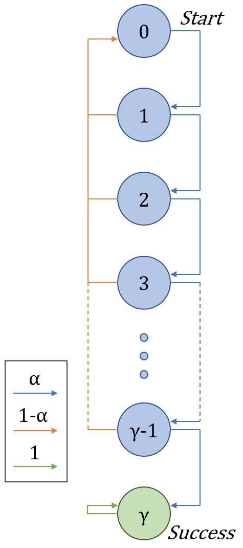
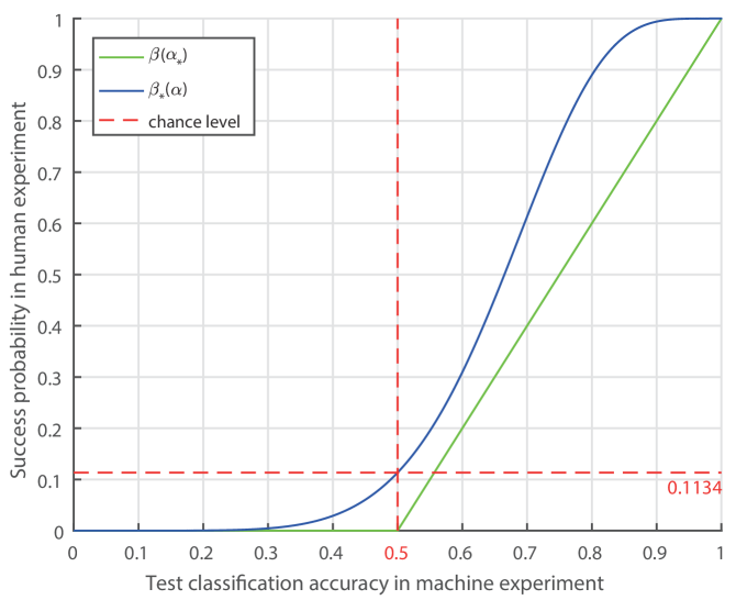
Figure 1: Reinterpretation of machine performance with the success probability $\beta_{*}(\alpha)$ for comparison with the human data. A machine agent of a test classification accuracy $\alpha$ attending a human experiment can be modelled as a discrete Markov chain (as the diagram on the left), where $Q_{k}(N)$ is the probability of the $k$ correct classifications in a row at the $N$-th step. As a success in the human experiment of Fleuret et al. (2011) required 7 correct classifications in a row by seeing up to 35 examples, $\beta_{*}(\alpha)=Q_{7}(35)$ is the probability of the machine agent to succeed in the human experiment (the blue curve in the graph on the right). The detailed derivation can be found in Section 5. The chance level of $\alpha$ is $50\%$, and that of $\beta_{*}(\alpha)$ is approximately $11.34\%$. Stabinger et al. (2016) reinterpreted the human performance by $\alpha_{*}(\beta)$ with $\beta=[2\alpha_{*}-1]_{+}$ (the green curve in the graph on the right), which effectively overestimated the human performance and underestimated the machine performance.

2.3 Grouping SVRT problems by core characteristics

Fleuret et al. (2011) plotted for the 23 problems the mean number of the trials before a human subject successfully detected the classification rule and the number of unsuccessful subjects, showing that there were 4 problems relatively difficult to human. In these problems, no less than 7 out of the 20 subjects were unsuccessful ($\beta<70\%$), which also took on average more than 12 images for the successful subjects before detecting the classification rules while the average is less than 7 for all other problems. In contrast, AdaBoost yielded a test error over 10% ($\alpha<90\%$) in 13 out of the 23 problems, when trained on 10,000 examples. Ellis et al. (2015) considered a problem as solved by machines if $\alpha\geq 90\%$, calculated the correlations between individual machines and human performance (i.e., the Pearson’s $r$ between $\alpha$ and $\beta$ for each machine agent), and remarked that their PS classifier Sasquatch was the best machine agent, comparing to AdaBoost and ConvNet, in terms of the number of solved problems and the correlation to the human performance.

As pointed out by Kim et al. (2018), however, comparing the number of solved problems is not a good idea for the general comparison between human and machine performance on SVRT. If a machine agent is able (or unable) to solve some problem, it is highly likely it would succeed (or fail) in similar problems. The 23 problems could contain many easy (or difficult), similar problems for this agent, because the original 23 problems were arbitrarily designed. Moreover, these relatively high (or low) machine accuracy might have uncorrected impact on the Pearson’s $r$, which is known to be not robust with respect to outliers, especially when sample size is small and non-normal; in the statistical analysis on the correlation between human and machine accuracies by Ellis et al. (2015), there are effectively only 23 data points. In order to freely control the generation of SVRT-like problems, Kim et al. (2018) proposed the PSVRT, so that they could systematically investigate the correlations between the parameters that modulate the image variability and the performance of their CNNs. Specifically, they firstly sorted the original 23 SVRT problems according to their CNN performances, noticing that their CNNs were good at the SR problems but poor at the SD problems. Then they developed the PSVRT which could generate random images based on to two core parameters, shape sizes (relative to image size) and number of shapes, modulating SR and SD respectively (Kim et al., 2018).

Based on the information encoded by image parsings and inspired by the idea of SD and SR, we propose to group SVRT problems into different types with respect to their core characteristics for classification, considering only two aspects of classification features, namely shape specification (SS) and location relation (LR). In particular, we assume four levels of complexity in both SS and LR, which are summarised in Table 2. With respect to SS, a classification rule can only rely on the core characteristics whether two shapes are similar in size ($SS=1$), or whether they are identical ($SS=2$) or identical under similarity transformations ($SS=3$). Any other geometric transformation would effectively change shape identities and reduce identical shapes to completely different shapes, because all shapes are randomly generated. In such cases, the classification rule is independent of shape specification ($SS=0$). Thus, the four levels of SS complexity characterise in principle all possible individual random shapes.

With respect to LR, a classification rule not based on a trivial, isolating relation ($LR=0$) either takes shape coordinates into account ($LR=2$ or $3$) or not ($LR=1$, a non-trivial topological relation). Generally on a two-dimensional plane, there exists only four topological relations between two shapes of finite area: isolating (the trivial one), bordering, containing and intersecting (Egenhofer and Franzosa, 1991). As the SVRT generator was designed to produce non-intersecting, random contours to avoid ambiguity in detecting shape identities, the lowest two levels of LR ($LR=0$ and $1$) exhaust all possible pairwise topological relations, which implicitly induce all possible topological relations among shapes in an image. In the cases when specific shape coordinates contribute to the core characteristics for classification, we assume that a non-linear relation in the shape coordinates ($LR=3$) is harder than a linear one ($LR=2$). This assumption is made based on the fact that PS processes non-linear numerical expressions much slower than linear ones, because the underlying algorithm for non-linear arithmetics is different from and more difficult than linear arithmetics (Bjørner et al., 2018). In addition, a pattern determined by a linear relation is also seemingly easier for human to detect, as shapes are likely to form a regular pattern, e.g., aligning in a line or at the corners of a square. Thus, the four levels of LR cover in principle all possible location relations among shapes.

In summary, we can group any SVRT problems into $15=4\times 4-1$ types in total according to SS and LR (no problem can have $SS=LR=0$). In order to solve problems of a particular type, the same type of features are necessary for any human or machine; we call such information the core characteristics for classification. Since the core characteristics ignores any features shared by both categories, the pair of $(SS,LR)$ qualitatively characterises the lowest amount of information necessary for classification.

SS	Shape specification
0	All shapes are completely different.
1	Some shapes are not identical but similar in size to one another.
2	Some shapes are identical to one another.
3	Some shapes are identical to one another under similarity transformations (i.e., scaling, reflection, rotation).
LR	Location relation
0	All shapes have a default, isolating relation.
1	Some shapes have a topological relation (i.e., a bordering or containing relation).
2	Some shapes have a linear relation in their coordinates (e.g., shapes aligned in a line/parallelogram).
3	Some shapes have a non-linear relation in their coordinates (e.g., equidistances between shapes).

Table 2: Definitions of the four levels of complexity with respect to SS and LR. All shapes are randomly generated contours with no intersections (there is at least 1 pixel between two contours). Thus, the default, null relation between two shapes corresponds to $SS=LR=0$, and a problem cannot belong to this null type because otherwise no classification rule exists.

The 23 original SVRT problems can be grouped into 8 types as shown in Table 3. It is worth noting that the core characteristics for classification is only necessary but not sufficient for classification; in other words, although different problems of the same type require common core characteristics, their classification rules are not necessarily identical. For example, the classification rule of problem #9 depends on whether the location of a larger shape lies between two smaller ones, while problem #13 depends on whether the relative locations of a larger shape with respect to a smaller one in two pairs are identical (i.e., whether there are two identical meta-shapes, each consisting of a larger and a smaller one). In addition, SS and LR can be correlated to each other in an image to some extent, whereas they seem conceptually independent to each other. For example, detecting whether two shapes have a bordering relation ($LR=1$) solves problem #2, while calculating how close their coordinates are can also be useful ($SS=2$), because the smaller shape is always inside the larger one and with a high probability it lies about the centre of the larger shape if not having a bordering relation. We assume problem #2 belonging to type $(SS,LR)=(0,1)$ rather than $(SS,LR)=(2,0)$, and the same idea applies and determines problem types for similar situations. Moreover, there are some disagreements between our SS-LR grouping and the SD-SR sorting by Kim et al. (2018), whereas the idea of SD is similar to SS as they both describe indivdual shapes. They sorted problem #6, #9, #12, #13 and #17 into the purely LR type, while we consider SS important for solving these 5 problems. For example, solving problem #9 clearly requires the core characteristics of shape sizes, which we believe is a characteristic of individual shapes rather than spatial relations between them.

LR	3		#12	#6, #17
	2	#10, #14, #18	#9, #13
	1	#2, #3, #4, #11, #23		#8
	0			#1, #5, #7, #15, #19, #20, #21, #22	#16
		0	1	2	3
		SS

Table 3: Different types of the original 23 SVRT problems. The problems are grouped by the core characteristics for classification defined in Table 2.

3 Results

3.1 Baseline Adaboost performance with correct parsings

As pointed out in Section 2.1, the image parsings obtained by the Sasquatch parser contained systematic errors in shape identity. They encoded no information of shape reflection, which is necessary for problem #16 and #20. In problem #21, rotated and rescaled shapes were assigned different shape identities unless the transformations were trivially small. Occassionally in problem #2, #3 and #11 when the shapes in contact were too close to one another, the parsings contained tiny shapes that should not exist; such glitchy shapes were in fact the random spaces well bounded by other shapes.

Parsing type	Sasquatch	Corrected		Error type in Sasquatch parsings
Training size	20		1000
Test size	80		1000
#2	51.25%	57.50%	59.90%	Extra glitchy shapes
#3	68.75%	50.00%	51.80%
#11	100.00%	100.00%	100.00%
#16	95.00%	100.00%	100.00%	Incorrect shape identity
#20	50.00%	100.00%	100.00%
#21	52.50%	38.75%	47.40%

Table 4: AdaBoost performance with Sasquatch and our corrected parsings. For the problems not listed here, the Sasquatch parsings are correct, and thus no significant performance differences can be seen comparing to our parsings. However, even for the listed problems that the Sasquatch parsings contain errors, only in problem #20 the performance difference can be seen.

Correcting these errors in the parsings, we expected the machine performance to increase for these problems. However, the performance of AdaBoost was boosted only in problem #20 (see Table 4). It is worth noting that, while the Sasquatch parsings failed to serve AdaBoost well in problems #20, they led to decent performance in problem #16. Although they were blind to shape reflection in both problem #16 and #20, it treated reflected shapes as different shapes and thus the classifcation rule of problem #16 changed from ‘whether shapes are reflected’ to ‘whether shapes are identical’, which coincidentally resulted in an indifferent performance. Meanwhile, this reflection blindness resulted in a complete failure in problem #20, because the classification rule depends on whether shapes are identical or not and this information was unretrievable in the Sasquatch parsings. Since extra glitchy shapes appeared infrequently in problem #2, #3 and #11, the performance were not changed significantly.

Since the number of stumps is essentially the only parameter that determines the final performance of AdaBoost (whereas there is a tradeoff in the learning efficiency for the learning rate or the base boosting algorithm) (Pedregosa et al., 2011), we conducted the experiments for 10, 100, 1,000 or 10,000 stumps and found the results extremely similar except for 10 stumps (and thus reported only the results for 10,000 stumps in Table 4). Both Sasquatch and our parsings are in general poor higher-level representations for AdaBoost; in fact, it yielded worse performance on such parsings than on features extracted directly from raw images (Fleuret et al., 2011; Ellis et al., 2015).

3.2 Improved PS performance with corrected parsings

By correcting the parsings, the performance of the PS classifier was boosted from the chance level to nearly the perfect in problems #20 and #21, while it was similar in other problems (see Figure 2 and Table LABEL:tab:Summary-of-performance for more details). The PS performance is highly dependent on the parsings, which is one reason for grouping the SVRT into different types as any parsing should in principle encode all necessary information for classification (see Section 2.3).

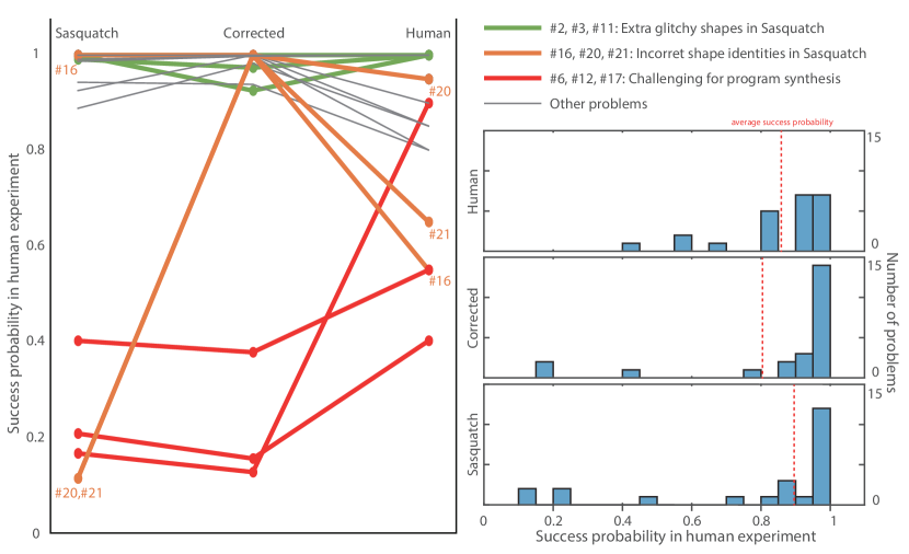
Figure 2: The program synthesis performance with the Sasquatch and our corrected parsings. The machine performance $\alpha$ is reinterpreted with $\beta_{*}(\alpha)$ by Figure 1B. The three histograms summarise the corresponding distributions of $\beta$ and $\beta_{*}(\alpha)$, where the averages are $86.30\pm 3.55\%$ for the human data, $81.40\pm 7.01\%$ for the Sasquatch parsings and $88.99\pm 5.62\%$ for the corrected parsings. By modifying the representation of image parsings, the machine performance were significantly enhanced in problem #20 and #21. Although the machine performance achieved, even surpassed, the human performance at many tasks, it was noticeably poor in problems #6, #12 and #17 (whose classification rule is dependent on equidistance relations between shapes). The human performance was calculated from the original data in Fleuret et al. (2011), and the machine performance of Sasquatch was reproduced by the code made public by Ellis et al. (2015) at https://github.com/ellisk42/sasquatch.

Other than the performance measured by the statistics ($\alpha$ or $\beta_{*}(\alpha)$), we also consider the performance of the PS classifier was improved in the sense of interpretability, which is one of the main advantages of the PS approach. Similar to the discussion on the AdaBoost performance, the PS classifier achieved decent performance with both the Sasquatch and our parsings in problem #16. However, the synthesized programs in the two cases were different. With the incorrect Sasquatch parsings, the program for the positive category was to firstly draw a group of three shapes and then another group; within either group the shapes were identical. With our corrected parsings, the program was to draw six identical shapes with three of them reflected.

Although the performance of the PS classifier was improved with the corrected parsings, achieving even surpassing human performance in many problems, it was relatively poor in problem #17 and merely above chance level in problem #6 and #12. The PS performance on these three problems rely on the most complex core characteristics for classification ($LR=3$) as equidistance between shapes (a non-linear relation in the shape coordinates) are involved. Although there was no constraint for the PS classifier to access the coordinate information in the parsings, its performance was inferior to the human level.

We did not attempt to re-engineer the parsings to encode the distance information directly. Although the PS classifier could conduct linear arithmetics over the distances rather than non-linear ones over the coordinates, saving some computational expense, the re-engineering would be at a huge cost in a combinatorial increase in the input sizes, which the PS classifier could not afford because it scales poorly with the input dimensionality. Moreover, even if the re-engineered parsings had resulted in a decent performance in the three problems, it could still be difficult for the classifier to generalise to unseen problems, as they encode only the pieces of information according to explicit human instructions. For example, we did not extract the information of shape rotation for the parsings, because it is not the core characteristics for classification in all the 23 problems. Thus, it is straightforward to design a new SVRT problem #101, which would be unsolvable problem for the PS classifier due to the rotation blindness of parsings, but not impossible for human subjects: all images in both categories contain two shapes; in one category the two shapes are identical, while in the other category the two shapes become identical after rotating.

In summary, we corrected the parsings so that they contain in principle all possible core characteristics for classification, which did lead to some improvement in the PS performance on many, but not all, SVRT problems.

3.3 Challenging problems for humans and machines

Next, we compared the human and machine performance on the orignal 23 SVRT problems across the 8 different types to which they belong (see Table 3). For compactness, we took the best CNN performance reported in Stabinger et al. (2016); Kim et al. (2018) as their performance were similar on most of the problems (see Table LABEL:tab:Summary-of-performance for the detailed data). By averaging the performance on different problems within each type, we obtained human and machine performance ($\beta$ and $\beta_{*}(\alpha)$) with respect to different levels of SS and LR as shown in Figure 3. In general, problem types on the left or lower in this $(SS,LR)$ plane are more complex than those on the right or upper in terms of the core characteristics for classification. Although the humans, the best CNN and the PS classifier with our corrected parsings actually yielded great performance in most of the problem types, they exposed their weaknesses when facing some problems types. The human performance was relatively poor in $(SS,LR)=(2,3)$ and $(SS,LR)=(3,0)$. The best CNN failed in $(SS,LR)=(2,0)$. The performance of the PS classifier with the correct parsings in $(SS,LR)=(1,3)$ and $(SS,LR)=(2,3)$ was not significantly better than the chance level.

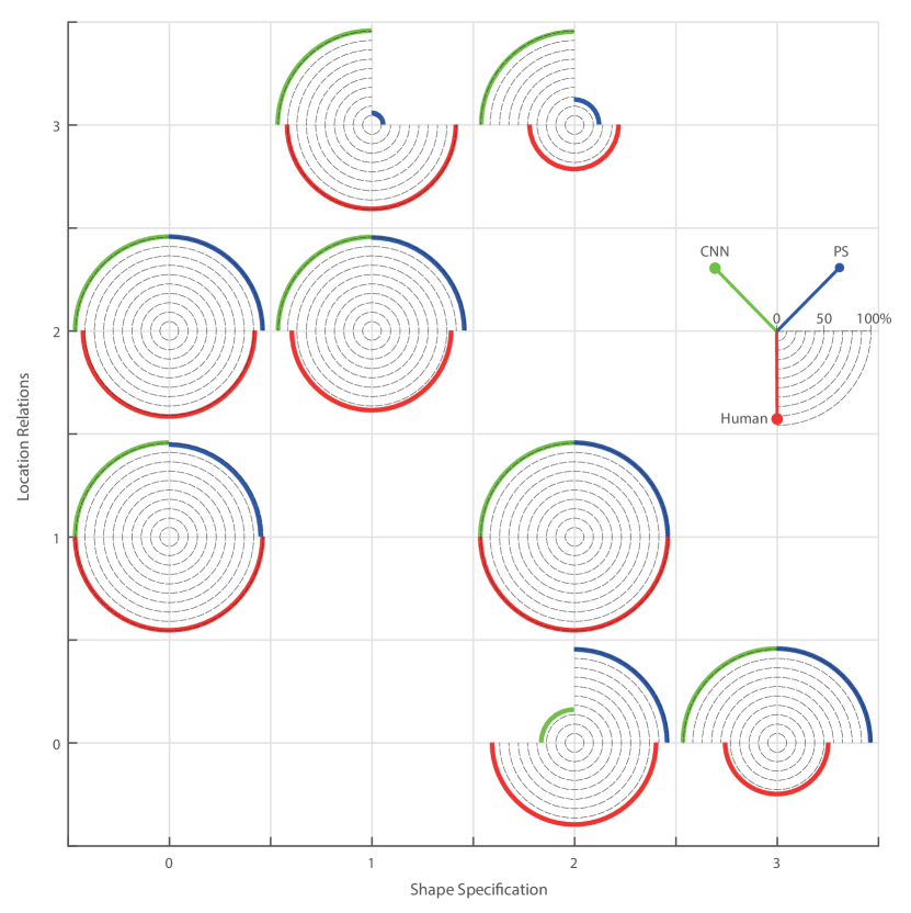
Figure 3: Comparison between human and machine (the best CNN and the PS classifier) performance on different groups of the SVRT problems. The group performance is depicted in propotion to the radii of the arcs.

As discussed in Section 3.2, the PS classifier failed to achieve a decent performance because it could not detected the equidistance relations between shapes, whereas the corrected parsings in principle provided it with the information to calculate such relations. The problem types of $LR=3$ are challenging to the PS classifier because non-linear arithmetics could be difficult to its underlying theorem prover to verify.

The best CNN was worst in the problem type of $(SS,LR)=(2,0)$, which means it is difficult for the CNNs to detect identical shapes within an image. This limitation of CNNs was thoroughtly studied by Kim et al. (2018). However, the performance was high in more difficult problem types of $(SS,LR)=(3,0)$, $(2,1)$ and $(2,3)$. The great performance in the type of $(SS,LR)=(3,0)$ was only due to LeNet, as its test accuracy is nearly perfect while that is poor for GoogLeNet and vanilla CNNs (see Table LABEL:tab:Summary-of-performance) (Stabinger et al., 2016; Kim et al., 2018). In contrast, they all yielded decent performance in the problem types of $(SS,LR)=(2,1)$ and $(2,3)$, specifically, on problem #6, #8 and #17.

The human performance could be an evidence showing that it was sensible for us to group the SVRT problems into these types. With an increase in the levels of either SS or LR, it required a human to extract more core characteristics for classification, making the problems more difficult. Other than problem #6, #16 and #17, which lie on the most top and right on this $(SS,LR)$ plane and thus yielded the worst 3 human results out of the 23 problems, we also remark that problem #21 was the next most challenging problem for many humans. In contrast, the human performance was nearly perfect on problem #19 and #20, whereas the classification rules of these 3 problems are seemingly alike in words and all belong to $(SS,LR)=(0,2)$. There are always two shapes in an image, for the positive category the two shapes are identical up to a similarity transformation, scaling for problem #19, reflection for problem #20 and rotation for problem #21, and for the negative category the two shapes are simply different.

In summary, according to our grouping by SS and LR, we found that finding non-linear relations in shape coordinates are the most challenging to the PS classifier, detection of identical shapes to the CNNs, and complex core characteristics for classification to the human subjects, whereas some differences between problems within the same types might have been overlooked.

3.4 Few-shot learning by PS classifier

One advantage of the PS classifier is its capability of learning from a small set of examples (Ellis et al., 2015); in particular, data in the previous figures were obtained by testing the classifier after training it with 3 positive and 3 negative examples. By varying the number of pairs $t$, the test accuracy $\alpha(t)$ is effectively the learning curve of the PS classifier, which is depicted in Figure 4 for all the original 23 SVRT problems. Although the PS classifier never achieved decent performance on problem #6, #12 and #17, it started to make correct classifications consistently if not perfectly in many other problems after seeing no more than 6 pairs of positive and negative examples. Comparing to the other ML techniques (e.g., AdaBoost, SVM and CNNs), the PS classifier needed a extremely small training set.

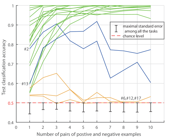
Figure 4: Learning curves of the PS classifier for the 23 tasks. The classifier reached optimal performance on many tasks after learning a few examples (in green). However, noticeable declines were observed for task #2 and #13 (in blue), which was caused by incorrect image parsings. Moreover, the classifier struggled at about chance level for task #6, #12, and #17 regardless of the number of the training examples (in orange). The classification rules of these three tasks are all dependent on equidistance relations between shapes, and the program synthesizer was unable to contruct optimal programs encoding such relations. Standard errors were calculated for all the data points, but only the maximal one for each size of training sets is depicted to avoid messy plots. When the accuracies approach $100\%$ (for many green curves), the corresponding standard errors drop to $0\%$.

However, a noticeable decline in the performance was observed for problem #2 and #13. This behaviour of PS was essentially caused by its formal verification nature . As any program can be synthesized to instantiate all the training images, an insignificant but misleading, random variability in the image parsings might be treated incorrectly as the core characteristics for classification, which weakens the program in generalising to unseen images. Moreover, if such misleading variability is ever taken into account by PS, it becomes one of the logical premises of the program. In other words, its impact cannot be removed or reduced. With an increasing number of training examples, the probability of at least one appearance of such random mistakes grows rapidly, which makes the PS classifier less likely to achieve high performance. In contrast, a statistical ML model (e.g., CNNs) may suffer a deterioration in its performance due to overfitting, which might also be a result of too powerful a model and too small a training set. However, a statistical model is only penalised by the deviation between its predication and the true label. As the frequency of such misleading variability was presumbly constant, its impact could be balanced out given more input data. In summary, more data could be beneficial to the generalisation ability of a statistical ML classifier. However, the same thing might be destructive to that ability of a PS classifier, unless the data (the training image parsings) are completely free of random mistakes.

4 Discussion

In this paper we have proposed a quantitative reintepretation of the human and machine performance on each SVRT problem for a fair comparison despite the differences in the experimental protocols. We have also grouped the problems into different types according to their core characteristics for classification, so that we could analyse and compare the human and machine performance on all the SVRT problems in a systematic manner despite of the arbitrary design of the original problems.

We confirmed with AdaBoost that the classification based on the parsings did not make the SVRT trivial, while incorrect parsings could make a problem unsolvable. The PS performance was dependent on the quality of the images parsings. With the corrected parsings, we improved the general performance on the original SVRT problems. However, the PS classifier still failed to detect equidistance relations in problem #6, #12 and #17, whereas it had access to the shape coordinates and was able to construct a program including a command encoding distances (computed from the coordinates). We also conducted the machine experiments on these problems with the time limit of the synthesizer set to be 10 times and even 100 times larger than the original one. No improvement in the performance was observed. We believe the failure is essentially due to combinatorially complexity increase in the non-linear verification in SMT. Movement is the only command in the synthesizer that is non-linear in general because a displacement is calculated from a moving distance and an orientation angle, which happens to be linear when there is only one initial angle. Thus, the PS classifier could solve, for example, problem #13 but not #12. It would also fail to generalise to other problems involving distances according to our grouping of the problems, unless a substaintially larger computational power could be deployed.

We grouped the problems based on the core characteristics for classification. The complexity level of the core characteristics was qualitatively ranked in the two aspects of SS and LR, while the complexity of the real classification rules could be completely different. In fact, the PS classifier chooses optimal programs by its evaluator measuring the complexity of constructed programs. We did not group the problems by the classification rules, because the core characteristics is more objective. The complexity of programs is only defined for the PS classifier. Humans might deduce different rules for the same category due to individual differences, especially when the images appear complicated. It is also not trivial for human to interpret a hyperplane found by AdaBoost or SVM or latent variables of a well-trained CNN, whereas they are virtually the classification rules to the machine agents. As the classification rules had to be found from the core characteristics, it was expected that the problems of higher SS and LR should on average yield no better performance than those of a lower SS and LR. However, we noted that the CNNs were better in the problem types of $(SS,LR)=(2,1)$ and $(2,3)$ than $(2,0)$. One possible explanation could be the correlation between SS and LR, whereas conceptually they might seem independent. Imposing more or stronger constraints solely on the locations of identical shapes might have made the entire image more regular, resulting in a spatial pattern that could be more easily detected by the CNNs without even noticing which shapes were identical. This argument would be consistent with the point of view of Kim et al. (2018), as they considered problem #6 and #17 to be purely about LR.

On the contrary, the recent success of training ResNet50 (a variant of CNN) to a high performance on all the 23 SVRT problems by Borowski et al. (2019) demonstrated the ability of feedforward convolutional architectures to detect identical shapes, whereas some problem types might remain difficult. Thus, in terms of classification accuracy, a well-trained CNN is for now the best machine agent for the SVRT. However, decent machine performance does not necessarily imply a human-like concept being learnt by a machine (Borowski et al., 2019), while the PS approach is intepretable to human as constructed programs are counterpart to the classification rules, which might be associated to semantic memory in human brain. Considering its capability of unsupervised, few-shot learning, the PS approach is advantageous in some aspects, whereas scalability is a major, general limitation. Due to this inherent limitation, the PS performance has to be dependent on the quality of image parsings.

One of the most fundamental differences between the PS and the statistical ML classifier (e.g., AdaBoost, CNNs) is how much prior knowledge correlated to the SVRT is manually encoded into the machine. We consider such prior knowledge particularly worthy of discussion when comparing machine and human performance and when investigating human-like computation in machines. Despite the fact that the human subjects had never seen the SVRT previously as the images were randomly generated, the human subjects could hold some prior knowledge correlated to the SVRT before the experiment, perhaps because the images involve higher-level configurations that biological visiual systems can perceive effortlessly due to evolution (Fleuret et al., 2011). In contrast, the statistical ML classifiers were trained from scratch (Fleuret et al., 2011; Ellis et al., 2015; Stabinger et al., 2016; Kim et al., 2018; Borowski et al., 2019), holding little prior knowledge except that for the general purpose of visual recognition. The SVRT images are known to consist of black and white pixels only; AdaBoost and SVM were based on some feature extractors; and all the CNNs deployed filters assuming translational symmetry. Although transfer learning is a common recipe for filling the gap of such prior knowledge to achieve few-shots learning in many ML contexts (Pan and Yang, 2009; Yosinski et al., 2014), it is not a promising solution to the SVRT, because without careful choice of model parameters they cannot perform decent classifications even after being trained on thousands of examples in some problem. Much more prior knowledge were manually encoded in the PS classifier. Although it assumes that in general the synthesizer can construct a program to instantiate any SVRT images in any category, it could be arguable whether the classifier is specially engineered for the original 23 problems. Our grouping thus became relevant in the analysis, because we could see which problem types, not individual problems, are trivial but which are challenging to machines.

Although Borowski et al. (2019) showed that their machine agent could solve all the 23 problems, the comparison between human and machine performance remains a complicated issue, because the protocols of the human and the machine experiments are different. Each human subject was learning and tested at the same time througout the experiment, while the machines are trained and tested separately. It is straightforward to simulate how a machine agent, capable of online learning, makes classifications as if it is in a human experiment. However, the issue of prior knowledge would become more relevant as one would have to decide to what degree the agent should be trained before implementing transfer learning and online learning. For the PS classifier, its poor performance on distance relations has to be fixed and a training strategy preventing its fast performance decline needs to be deployed.

The PS classifier is advantageous for its capability of unsupervised, few-shot learning, because the underlying theorem prover, Z3, performs symbolic computation using high level representation of images (i.e., parsings). For the same reason, it has a scalability problem and relies on the parsings, while the CNNs do not have such limitations. The different advantages and disadvantages of the symbolic and neural approaches suggests their combination might lead to greater machine performance, e.g., Ellis et al. (2018); Huang et al. (2018); Minervini et al. (2018); Selsam et al. (2018).

5 Appendix

5.1 Summary of the SVRT problems: example images, classification rules and problem types.

The original 23 SVRT problems were generated using our code, which was forked from Fleuret et al. [2011].

References

- Bjørner et al. [2018] Nikolaj Bjørner, Leonardo de Moura, Lev Nachmanson, and Christoph Wintersteiger. Programming Z3, 2018. URL http://http://theory.stanford.edu/~nikolaj/programmingz3.html.
- Borowski et al. [2019] Judy Borowski, Christina M Funke, Karolina Stosio, Wieland Brendel, Thomas S A Wallis, and Bethge Matthias. The notorious difficulty of comparing human and machine perception. In Proceedings of the Conference on Cognitive Computational Neuroscience, 2019.
- Cook [1971] Stephen A Cook. The complexity of theorem-proving procedures. In Proceedings of the third annual ACM symposium on Theory of computing, pages 151–158. ACM, 1971.
- Egenhofer and Franzosa [1991] Max J Egenhofer and Robert D Franzosa. Point-set topological spatial relations. International Journal of Geographical Information System, 5(2):161–174, 1991.
- Ellis et al. [2015] Kevin Ellis, Armando Solar-Lezama, and Josh Tenenbaum. Unsupervised learning by program synthesis. In Advances in Neural Information Processing Systems, pages 973–981, 2015.
- Ellis et al. [2018] Kevin Ellis, Lucas Morales, Mathias Sabl Meyer, Armando Solar-Lezama, and Joshua B Tenenbaum. Dreamcoder: Bootstrapping domain-specific languages for neurally-guided bayesian program learning. In Neural Abstract Machines and Program Induction Workshop at NIPS, 2018.
- Fleuret et al. [2011] François Fleuret, Ting Li, Charles Dubout, Emma K Wampler, Steven Yantis, and Donald Geman. Comparing machines and humans on a visual categorization test. Proceedings of the National Academy of Sciences, 2011.
- Huang et al. [2018] Daniel Huang, Prafulla Dhariwal, Dawn Song, and Ilya Sutskever. Gamepad: A learning environment for theorem proving. arXiv preprint arXiv:1806.00608, 2018.
- Kim et al. [2018] Junkyung Kim, Matthew Ricci, and Thomas Serre. Not-So-CLEVR: learning same–different relations strains feedforward neural networks. Interface focus, 8(4):20180011, 2018.
- Minervini et al. [2018] Pasquale Minervini, Matko Bosnjak, Tim Rocktäschel, and Sebastian Riedel. Towards neural theorem proving at scale. arXiv preprint arXiv:1807.08204, 2018.
- Pan and Yang [2009] Sinno Jialin Pan and Qiang Yang. A survey on transfer learning. IEEE Transactions on knowledge and data engineering, 22(10):1345–1359, 2009.
- Pedregosa et al. [2011] F. Pedregosa, G. Varoquaux, A. Gramfort, V. Michel, B. Thirion, O. Grisel, M. Blondel, P. Prettenhofer, R. Weiss, V. Dubourg, J. Vanderplas, A. Passos, D. Cournapeau, M. Brucher, M. Perrot, and E. Duchesnay. Scikit-learn: Machine learning in Python. Journal of Machine Learning Research, 12:2825–2830, 2011.
- Selsam et al. [2018] Daniel Selsam, Matthew Lamm, Benedikt Bünz, Percy Liang, Leonardo de Moura, and David L Dill. Learning a sat solver from single-bit supervision. arXiv preprint arXiv:1802.03685, 2018.
- Stabinger et al. [2016] Sebastian Stabinger, Antonio Rodríguez-Sánchez, and Justus Piater. 25 years of CNNs: Can we compare to human abstraction capabilities? In International Conference on Artificial Neural Networks, pages 380–387. Springer, 2016.
- Yosinski et al. [2014] Jason Yosinski, Jeff Clune, Yoshua Bengio, and Hod Lipson. How transferable are features in deep neural networks? In Advances in neural information processing systems, pages 3320–3328, 2014.