The Laplace transform of the integrated Volterra Wishart process

Abstract

We establish an explicit expression for the conditional Laplace transform of the integrated Volterra Wishart process in terms of a certain resolvent of the covariance function. The core ingredient is the derivation of the conditional Laplace transform of general Gaussian processes in terms of Fredholm’s determinant and resolvent. Furthermore, we link the characteristic exponents to a system of non-standard infinite dimensional matrix Riccati equations. This leads to a second representation of the Laplace transform for a special case of convolution kernel. In practice, we show that both representations can be approximated by either closed form solutions of conventional Wishart distributions or finite dimensional matrix Riccati equations stemming from conventional linear-quadratic models. This allows fast pricing in a variety of highly flexible models, ranging from bond pricing in quadratic short rate models with rich autocorrelation structures, long range dependence and possible default risk, to pricing basket options with covariance risk in multivariate rough volatility models.
Keywords: Gaussian processes, Wishart processes, Fredholm’s determinant, quadratic short rate models, rough volatility models.
MSC2010 Classification: 60G15, 60G22, 45B05, 91G20.

1 Introduction

We are interested in the $d\times d$ Volterra Wishart process $XX^{\top}$ where $X$ is the $d\times m$-matrix valued Volterra Gaussian process

$$X_{t} =g_{0}(t)+\int_{0}^{t}K(t,s)dW_{s},$$ (1.1)

for some given input curve $g_{0}:[0,T]\to{{\mathbb{R}}}^{d\times m}$, suitable kernel $K:[0,T]^{2}\to{\mathbb{R}}^{d\times d}$ and $d\times m$-matrix Brownian motion $W$, for a fixed time horizon $T>0$.

The introduction of the kernel $K$ allows for flexibility in financial modeling as illustrated in the two following examples. First, one can consider asymmetric (possibly negative) quadratic short rates of the form

$$r_{t}=\operatorname{tr}\left(X_{t}^{\top}QX_{t}\right)+\xi(t)$$

where $Q\in{\mathbb{S}}^{d}_{+}$, $\xi$ is an input curve used for matching market term structures and $\operatorname{tr}$ stands for the trace operator. The kernel $K$ allows for richer autocorrelation structures than the one generated with the conventional Hull and White (1990) and Cox, Ingersoll, and Ross (2005) models. Second, for $d=m$, one can build stochastic covariance models for $d$–assets $S=(S^{1},\ldots,S^{d})$ by considering the following dynamics for the stock prices:

$$dS_{t} =\operatorname{diag}(S_{t})X_{t}dB_{t}$$

where $B$ is $d$-dimensional and correlated with $W$. Then, the instantaneous covariance between the assets is stochastic and given by $\frac{d\langle\log S\rangle_{t}}{dt}=X_{t}X_{t}^{\top}\in{\mathbb{S}}^{d}_{+}$. When $d=m=1$, one recovers the Volterra version of the Stein and Stein (1991) or Schöbel and Zhu (1999) model. Here, singular kernels $K$ satisfying $\lim_{s\uparrow t}|K(t,s)|=\infty$, allow to take into account roughness of the sample paths of the volatility, as documented in Bennedsen et al. (2016); Gatheral et al. (2018). As an illustrative example for $d=m=1$, one could consider the Riemann-Liouville fractional Brownian motion

$$X_{t}=\frac{1}{\Gamma(H+1/2)}\int_{0}^{t}(t-s)^{H-1/2}dW_{s},$$ (1.2)

either with $H\in(0,1/2)$ to reproduce roughness when modeling the variance process, or with $H\in(1/2,1)$ to account for long memory in short rate models.

In both cases, integrated quantities of the form $\int_{0}^{\cdot}X_{s}X_{s}^{\top}ds$ play a key role for pricing zero-coupon bonds and options on covariance risk. In order to keep the model tractable, one needs to come up with fast pricing and calibration techniques. The main objective of the paper is to show that these models remain highly tractable, despite the inherent non-markovianity and non-semimartingality due to the introduction of the kernel $K$. For $w\in{\mathbb{S}}^{d}_{+}$, our main result (Theorem 3.3) provides the explicit expression for the conditional Laplace transform:

$${\mathbb{E}}\left[\exp\left(-\int_{t}^{T}\operatorname{tr}\left(wX_{s}X_{s}^{\top}\right)ds\right){\ \Big{|}\ }{\mathcal{F}}_{t}\right]=\exp\left(\phi_{t,T}+\int_{(t,T]^{2}}\!\operatorname{tr}\left(g_{t}(s)^{\top}\Psi_{t,T}(ds,du)g_{t}(u)\right)\right),\;\;\;\;$$ (1.3)

where $(\phi,\Psi)$ are defined by

$$\partial_{t}\phi_{t,T} =-m\int_{(t,T]^{2}}\operatorname{tr}\left(\Psi_{t,T}(ds,du)K(u,t)K(s,t)^{\top}\right),\quad\phi_{T,T}=0,$$ (1.4)

$$\Psi_{t,T}(ds,du) =-w\delta_{\{s=u\}}(ds,du)-\sqrt{w}R^{w}_{t,T}(s,u)\sqrt{w}dsdu,$$ (1.5)

with $g_{t}(s)={\mathbb{E}}[X_{s}|{\mathcal{F}}_{t}]$ the forward process, $C_{t}(s,u)={\mathbb{E}}[(X_{s}-g_{t}(s))(X_{u}-g_{t}(u))^{\top}|{\mathcal{F}}_{t}]$ the conditional covariance function, and $R^{w}_{t,T}:[0,T]^{2}\to{\mathbb{R}}^{d\times d}$ the Fredholm resolvent of $(-2\sqrt{w}C_{t}\sqrt{w})$ on $[0,T]$ given by

$$R^{w}_{t,T}(s,u)=-2\sqrt{w}C_{t}(s,u)\sqrt{w}-\int_{t}^{T}2\sqrt{w}C_{t}(s,z)\sqrt{w}R^{w}_{t,T}(z,u)dz,\quad t\leq s,u\leq T.$$

Using the integral operator $\mathbb{C}_{t}$ induced by the covariance kernel $C_{t}$, i.e. $(\mathbb{C}_{t}f)(s)=\int_{0}^{T}C_{t}(s,u)f(u)du$ for $f\in L^{2}\left([0,T],{\mathbb{R}}^{d\times m}\right)$, the Laplace transform can be re-expressed in explicit form

$${\mathbb{E}}\left[\exp\left(-\int_{t}^{T}\operatorname{tr}\left(wX_{s}X_{s}^{\top}\right)ds\right){\ \Big{|}\ }{\mathcal{F}}_{t}\right]=\frac{\exp\left(\langle g_{t},\sqrt{w}\left({\rm id}+2\sqrt{w}\mathbb{C}_{t}\sqrt{w}\right)^{-1}\sqrt{w}g_{t}\rangle_{L^{2}_{t}}\right)}{\det\left({\rm id}+2\sqrt{w}\mathbb{C}_{t}\sqrt{w}\right)^{m/2}}$$ (1.6)

where $\langle f,g\rangle_{L^{2}_{t}}=\int_{t}^{T}\operatorname{tr}\left(f(s)^{\top}g(s)\right)ds$ and $\det$ stands for the Fredholm determinant.

The Laplace transform is exponentially quadratic in the forward process $(g_{t})_{t\leq T}$, and cannot in general be recovered from that of finite dimensional affine Volterra processes introduced in Abi Jaber et al. (2019a), see Remark 2.1. We also mention that the models studied here are quadratic constructions of Gaussian processes and do not pose any difficulty regarding existence and uniqueness, in contrast for instance with conventional Wishart processes that go beyond squares of Gaussians, see Bru (1991).

Furthermore, we link $\Psi$ to a system of non-standard infinite dimensional backward Riccati equations in the general case of non-convolution kernels. This allows us to deduce a second representation of the Laplace transform for a special case of convolution kernels in the form

$$K(t,s)=k(t-s)\bm{1}_{s\leq t}\quad\mbox{ such that }\quad k(t)=\int_{{\mathbb{R}}_{+}}e^{-xt}\mu(dx),\quad t>0,$$

for some suitable signed measure $\mu$, showing, similarly to Cuchiero and Teichmann (2019); Harms and Stefanovits (2019), that the Volterra Wishart process can be seen as a superposition of possibly infinitely many conventional linear-quadratic models written on the infinite dimensional process

$$Y_{t}(x)=\int_{0}^{t}e^{-x(t-s)}dW_{s},\quad t\geq 0,\quad x\in{\mathbb{R}}_{+}.$$

In particular, this second representation not only allows us to recover the expressions for the Laplace transform derived in the aforementioned articles but, most importantly, provides an explicit solution for the corresponding infinite dimensional Riccati equations.

Although explicit, the expression for the Laplace transform is not known in closed form, except for certain cases. We provide two approximation procedures either by closed form solutions of conventional Wishart distributions (Section 2.3) or finite dimensional matrix Riccati equations stemming from conventional linear-quadratic models (Section 3.3). These approximations can then be used to price bonds with possible default risk, or options on covariance in multivariate (rough) volatility models by Laplace transform techniques (Section 4).

Literature Conventional Wishart processes initiated by Bru (1991) and introduced in finance by Gourieroux and Sufana (2003) have been intensively applied, together with their variants, in term structure and stochastic covariance modeling, see for instance Alfonsi (2015); Buraschi et al. (2010); Cuchiero et al. (2011, 2016); Da Fonseca et al. (2007, 2008); Gouriéroux et al. (2009); Muhle-Karbe et al. (2012). Conventional linear quadratic models have been characterized in Chen et al. (2004); Cheng and Scaillet (2007). Volterra Wishart processes have been recently studied in Cuchiero and Teichmann (2019); Yue and Huang (2018). Applications of certain quadratic Gaussian processes can be found in Benth and Rohde (2018); Corcuera et al. (2013); Harms and Stefanovits (2019); Kleptsyna et al. (2002). Gaussian stochastic volatility models have been treated in Gulisashvili (2018); Gulisashvili et al. (2019).

Outline In Section 2 we derive the Laplace transform of general quadratic Gaussian processes in ${\mathbb{R}}^{N}$, we provide a first approximation procedure by closed form expressions and link the characteristic exponent to non-standard Riccati equations. These results are then used in Section 3 to deduce the Laplace transforms of Volterra Wishart processes. We also provide a second representation formula for the Laplace transform together with an approximation scheme for a special class of convolution kernels. Section 4 presents applications to pricing: (i) bonds in quadratic Volterra short rate models with possible default risk; (ii) options on volatility for basket products in Volterra Wishart (rough) covariance models. Some technical results are collected in the appendices.

Notations For $T>0$, we define $L^{2}([0,T]^{2},{\mathbb{R}}^{N\times N})$ to be the space of measurable functions $F:[0,T]^{2}\to{\mathbb{R}}^{N\times N}$ such that

$$\int_{0}^{T}\int_{0}^{T}|F(t,s)|^{2}dtds<\infty.$$

For any $F,G\in L^{2}([0,T]^{2},{\mathbb{R}}^{N\times N})$ we define the $\star$-product by

$$(F\star G)(s,u)=\int_{0}^{T}F(s,z)G(z,u)du,\quad s,u\leq T,$$ (1.7)

which is well-defined in $L^{2}([0,T]^{2},{\mathbb{R}}^{N\times N})$ due to the Cauchy-Schwarz inequality. We denote by $F^{*}$ the adjoint kernel of $F$ in $L^{2}([0,T],{\mathbb{R}}^{N\times N})$, that is

$$F^{*}(s,u)=F(u,s)^{\top},\quad s,u\leq T.$$

For any kernel $F\in L^{2}([0,T]^{2},{\mathbb{R}}^{N\times N})$, we denote by $\mathbb{F}$ the integral operator from $L^{2}([0,T],{\mathbb{R}}^{N})$ into itself induced by the kernel $F$ that is

$$({\mathbb{F}}g)(s)=\int_{0}^{T}F(s,u)g(u)du,\quad g\in L^{2}([0,T],{\mathbb{R}}^{N}).$$ (1.8)

If $\mathbb{F}$ and $\mathbb{G}$ are two integral operators induced by the kernels $F$ and $G$ in $L^{2}([0,T]^{2},{\mathbb{R}}^{N\times N})$, then $\mathbb{F}\mathbb{G}$ is an integral operator induced by the kernel $F\star G$.

${\mathbb{S}}^{N}_{+}$ stands for the cone of symmetric non-negative semidefinite $N\times N$-matrices, $\operatorname{tr}$ denotes the trace of a matrix and $I_{N}$ is the $N\times N$ identity matrix. The vectorization operator is denoted by $\operatorname{vec}$ and the Kronecker product by $\otimes$, we refer to Appendix B for more details.

2 Quadratic Gaussian processes

Throughout this section, we fix $T>0$, $N\geq 1$ and let $Z$ denote a ${\mathbb{R}}^{N}$-valued square-integrable Gaussian process on a filtered probability space $(\Omega,{\mathcal{F}},({\mathcal{F}}_{t})_{t\leq T},{\mathbb{P}})$ with mean function $g_{0}(s)={\mathbb{E}}[Z_{s}]$ and covariance kernel given by $C_{0}(s,u)={\mathbb{E}}[(Z_{s}-g_{0}(s))(Z_{u}-g_{0}(u))^{\top}]$, for each $s,u\in[0,T]$. We note that $g_{0}$ and $C_{0}$ may depend on $T$, but we do not make this dependence explicit to ease notations.

2.1 Fredholm’s representation and first properties

Assume that $C_{0}$ is continuous in both variables. Then, there exists a kernel $K_{T}\in L^{2}([0,T]^{2},{\mathbb{R}}^{N\times N})$ and a $N$-dimensional Brownian motion $W$ such that

$$Z_{t}=g_{0}(t)+\int_{0}^{T}K_{T}(t,s)dW_{s},$$ (2.1)

for all $t\leq T$, see Sottinen and Viitasaari (2016, Theorem 12 and Example 2). In particular, $C_{0}=K_{T}\star K_{T}^{*}$, that is

$$C_{0}(s,u)=\int_{0}^{T}K_{T}(s,z)K_{T}(u,z)^{\top}dz,\quad s,u\leq T.$$

For any $t\leq s$, $Z_{s}$ admits the following decomposition

$$Z_{s}=g_{0}(s)+\int_{0}^{t}K_{T}(s,u)dW_{u}+\int_{t}^{T}K_{T}(s,u)dW_{u},$$ (2.2)

showing that conditional on ${\mathcal{F}}_{t}$, $Z_{s}$ is again a Gaussian process with conditional mean

$$g_{t}(s)={\mathbb{E}}[Z_{s}|{\mathcal{F}}_{t}]=g_{0}(s)+\int_{0}^{t}K_{T}(s,u)dW_{u},\quad t\leq s\leq T,$$

and conditional covariance function

$$C_{t}(s,u) ={\mathbb{E}}[(Z_{s}-g_{t}(s))(Z_{u}-g_{t}(u))^{\top}|{\mathcal{F}}_{t}]$$

$$=\int_{t}^{T}K_{T}(s,z)K_{T}(u,z)^{\top}dz,\quad\quad\quad t\leq s,u\leq T.$$ (2.3)

Again we drop the possible dependence of $g_{t}$ and $C_{t}$ on $T$, and we note in particular that for each $s,u\leq T$, $t\to C_{t}(s,u)$ is absolutely continuous on $[0,s\wedge u]$ with density

$$\dot{C}_{t}(s,u)=-K(s,t)K(u,t)^{\top},$$ (2.4)

and that the process $t\mapsto g_{t}(s)$ is a semimartingale on $[0,s)$ with dynamics

$$dg_{t}(s)=K_{T}(s,t)dW_{t},\quad t<s.$$

We are chiefly interested in the ${\mathbb{S}}^{N}_{+}$-valued process $ZZ^{\top}$. The following remark shows that, in general, $ZZ^{\top}$ cannot be recast as an affine Volterra process as studied in Abi Jaber et al. (2019a).

Remark 2.1.

To fix ideas, we set $g_{0}\equiv Z_{0}\in{\mathbb{R}}^{N}$. An application of Itô’s formula yields

$$g_{t}(s)g_{t}(s)^{\top} =Z_{0}Z_{0}^{\top}+\int_{0}^{t}K_{T}(s,u)K_{T}(s,u)^{\top}du$$

$$\quad+\int_{0}^{t}K_{T}(s,u)dW_{u}{g_{u}(s)}^{\top}+\int_{0}^{t}{g_{u}(s)}dW_{u}^{\top}K_{T}(s,u)^{\top},\quad t<s.$$

Taking the limit $s\to t$ leads to the dynamics

$$Z_{t}Z_{t}^{\top} =Z_{0}Z_{0}^{\top}+\int_{0}^{t}K_{T}(t,u)K_{T}(t,u)^{\top}du$$

$$\quad+\int_{0}^{t}K_{T}(t,u)dW_{u}{g_{u}(t)}^{\top}+\int_{0}^{t}{g_{u}(t)}dW_{u}^{\top}K_{T}(t,u)^{\top}.$$ (2.5)

This shows, that in general, because of the presence of the infinite dimensional process $t\mapsto g_{t}$ in the dynamics, $ZZ^{\top}$ does not satisfy a stochastic Volterra equation in the form

$$Y_{t}=Y_{0}+\int_{0}^{t}K(t,s)b(Y_{s})ds+\int_{0}^{t}\sigma(Y_{s})dW_{s}^{\top}K(t,s)^{\top}+\int_{0}^{t}K(t,s)dW_{s}\sigma(Y_{s})^{\top},$$

where $b,\sigma:{\mathbb{R}}^{N}\mapsto{\mathbb{R}}^{N\times N}$. For this reason, $ZZ^{\top}$ falls beyond the scope of the processes studied in Abi Jaber et al. (2019a). Except for very specific cases, for instance, when $K_{T}\equiv I_{N}$, we have $g_{u}(s)=Z_{u}$ for all $u<s$, and (2.5) reduces to the well-known dynamics of Wishart processes as introduced by Bru (1991).

Whence, the conditional Laplace transform of $ZZ^{\top}$ cannot be deduced from Abi Jaber et al. (2019a, Theorem 4.3). Nonetheless, it can be directly computed from Wishart distributions that we recall in Appendix A.

Theorem 2.2.

Fix $t\leq s\leq T$. Conditional on ${\mathcal{F}}_{t}$, $Z_{s}Z_{s}^{\top}$ follows a Wishart distribution

$$Z_{s}Z_{s}^{\top}\sim_{|{\mathcal{F}}_{t}}{\mbox{WIS}}_{N}\left(1/2,g_{t}(s)g_{t}(s)^{\top},2C_{t}(s,s)\right).$$

Further, for any $u\in{\mathbb{S}}^{N}_{+}$, the conditional Laplace transform reads

$${\mathbb{E}}\left[\exp\left(-Z_{s}^{\top}uZ_{s}\right){\ \Big{|}\ }{\mathcal{F}}_{t}\right]=\frac{\exp\left(-g_{t}(s)^{\top}u\left(I_{N}+2C_{t}(s,s)u\right)^{-1}g_{t}(s)\right)}{\det\left(I_{N}+2C_{t}(s,s)u\right)^{1/2}}.$$ (2.6)

Proof.

Fix $t\leq s\leq T$, conditional on ${\mathcal{F}}_{t}$, it follows from (2.2) that $Z_{s}$ is a Gaussian vector in ${\mathbb{R}}^{N}$ with mean vector $g_{t}(s)\in{\mathbb{R}}^{N}$ and covariance matrix $C_{t}(s,s)\in{\mathbb{R}}^{N\times N}$. The claimed result now follows from Proposition A.1. ∎

In particular, if $N=1$, $t=0$ and $s=T$, one obtains the well-known chi-square distribution

$${\mathbb{E}}\left[\exp\left(-uZ^{2}_{T}\right)\right]=\frac{\exp\left(\frac{-ug_{0}(T)^{2}}{1+2uC_{0}(T,T)}\right)}{\left(1+2uC_{0}(T,T)\right)^{1/2}},\quad u\geq 0.$$

The computation of the Laplace transform for the integrated squared process is more involved and is treated in the next subsection.

2.2 Conditional Laplace transform of the integrated quadratic process

We are interested in computing the conditional Laplace transform

$${\mathbb{E}}\left[\exp\left(-\int_{t}^{T}Z_{s}^{\top}wZ_{s}ds\right){\ \Big{|}\ }{\mathcal{F}}_{t}\right],\quad w\in{\mathbb{S}}^{N}_{+},\quad t\leq T.$$ (2.7)

For $t=0$ and for centered processes, such computations appeared several times in the literature showing that the quantity of interest can be decomposed as an infinite product of independent chi-square distributions, see for instance Anderson and Darling (1952); Cameron and Donsker (1959); Varberg (1966). The same methodology can be readily adapted to our dynamical case and makes use of the celebrated Kac–Siegert/Karhunen–Loève representation of the process $Y=\sqrt{w}Z$ whose conditional covariance function is $C^{w}_{t}=\sqrt{w}C_{t}\sqrt{w}$, see Kac and Siegert (1947); Karhunen (1946); Loeve (1955). For this, we fix $t\leq T$, we consider the inner product on $L^{2}([t,T],{\mathbb{R}}^{N})$ given by

$$\langle f,g\rangle_{L^{2}_{t}}=\int_{t}^{T}f(s)^{\top}g(s)ds,\quad\quad f,g\in L^{2}([t,T],{\mathbb{R}}^{N}),$$

and we assume that $C_{t}$ is continuous in both variables. By definition, the covariance kernel $C^{w}_{t}$ is symmetric and nonnegative in the sense that

$$C^{w}_{t}(s,u)=C^{w}_{t}(u,s)^{\top},\quad s,t\leq T,$$

and

$$\int_{t}^{T}\int_{t}^{T}f(s)^{\top}C^{w}_{t}(s,u)f(u)duds\geq 0,\quad f\in L^{2}([t,T],{\mathbb{R}}^{N}).$$

An application of Mercer’s theorem, see Shorack and Wellner (2009, Theorem 1 p.208), yields the existence of a countable orthonormal basis $(e^{n}_{t,T})_{n\geq 1}$ in $L^{2}([t,T],{\mathbb{R}}^{N})$ and a sequence of nonnegative real numbers $(\lambda^{n}_{t,T})_{n\geq 1}$ with $\sum_{n\geq 1}\lambda^{n}_{t,T}<\infty$ such that

$$C^{w}_{t}(s,u) =\sum_{n\geq 1}\lambda_{t,T}^{n}e_{t,T}^{n}(s)e_{t,T}^{n}(u)^{\top},\quad t\leq s,u\leq T,$$ (2.8)

and

$$\int_{t}^{T}C^{w}_{t}(s,u)e^{n}_{t,T}(u)du=\lambda^{n}_{t,T}e_{t,T}^{n}(s),\quad t\leq s\leq T,\quad n\geq 1,$$ (2.9)

where the dependence of $(e_{t,T}^{n},\lambda^{n}_{t,T})$ on $w$ is dropped to ease notations. This means that $(\lambda^{n}_{t,T},e^{n}_{t,T})_{n\geq 1}$ are the eigenvalues and the eigenvectors of the integral operator $\sqrt{w}\mathbb{C}_{t}\sqrt{w}$ from $L^{2}([t,T],{\mathbb{R}}^{N})$ into itself induced by $C_{t}^{w}$:

$$(\sqrt{w}\mathbb{C}_{t}\sqrt{w}f)(s)=\int_{t}^{T}C^{w}_{t}(s,u)f(u)du,\quad t\leq s\leq T,\quad f\in L^{2}([t,T],{\mathbb{R}}^{N}).$$

As a consequence of Mercer’s theorem, conditional on ${\mathcal{F}}_{t}$, the process $Y$ admits the Kac–Siegert representation

$$Y_{s} =\sqrt{w}g_{t}(s)+\sum_{n\geq 1}\sqrt{\lambda_{t,T}^{n}}\xi^{n}e_{t,T}^{n}(s),\quad t\leq s\leq T,$$ (2.10)

where, conditional on ${\mathcal{F}}_{t}$, $(\xi_{n})_{n\geq 1}$ is a sequence of independent standard Gaussian random variables, see Shorack and Wellner (2009, Theorem 2 p.210 and the comment below (14) on p.212). We now introduce the quantities needed for the computation of (2.7) in Theorem 2.3 below. We denote by ${\rm id}$ the identity operator on $L^{2}([t,T],{\mathbb{R}}^{N})$, i.e. $({\rm id}f)(s)=f(s)$, by $({\rm id}+2\sqrt{w}\mathbb{C}_{t}\sqrt{w})^{-1}$ the integral operator generated by the kernel

$$\sum_{n\geq 1}\frac{1}{1+2\lambda_{t,T}^{n}}e_{t,T}^{n}(s)e_{t,T}^{n}(u)^{\top},$$ (2.11)

and we set

$$\det({\rm id}+2\sqrt{w}\mathbb{C}_{t}\sqrt{w}):=\prod_{n\geq 1}\left({{1+2\lambda_{t,T}^{n}}}\right).$$ (2.12)

The last expression is well defined due to the convergence of the series $(\sum_{n=1}^{m}\lambda^{n}_{t,T})_{m\geq 1}$ and the inequality

$$1+2\sum_{n=1}^{m}\lambda^{n}_{t,T}\leq\prod_{n=1}^{m}\left(1+2\lambda^{n}_{t,T}\right)\leq\exp\left(2\sum_{n=1}^{m}\lambda^{n}_{t,T}\right),\quad m\geq 1.$$

Theorem 2.3.

Fix $w\in{\mathbb{S}}^{N}_{+}$ and $t\leq T$. Assume that the function $(s,u)\mapsto C_{t}(s,u)$ is continuous. Then,

$${\mathbb{E}}\left[\exp\left(\!-\!\int_{t}^{T}Z_{s}^{\top}wZ_{s}ds\right)\!\!{\ \Big{|}\ }\!{\mathcal{F}}_{t}\right]=\frac{\!\exp\left(-\langle g_{t},\!\sqrt{w}\left({\rm id}+2\sqrt{w}\mathbb{C}_{t}\!\sqrt{w}\right)^{-1}\!\!\sqrt{w}g_{t}\rangle_{L^{2}_{t}}\right)}{\det\left({\rm id}+2\sqrt{w}\mathbb{C}_{t}\sqrt{w}\right)^{1/2}}.\quad\;\;\;$$ (2.13)

Proof.

Fix $t\leq T$. Parseval’s identity gives $\langle\sqrt{w}g_{t},\sqrt{w}g_{t}\rangle_{L^{2}_{t}}=\sum_{n\geq 1}\langle\sqrt{w}g_{t},e^{n}_{t,T}\rangle_{L^{2}_{t}}^{2}$ so that

$$\int_{t}^{T}Z_{s}^{\top}wZ_{s}ds=\langle Y,Y\rangle_{L^{2}_{t}}=\sum_{n\geq 1}\left(\sqrt{\lambda_{t,T}^{n}}\xi^{n}+\langle\sqrt{w}g_{t},e^{n}_{t,T}\rangle_{L^{2}_{t}}\right)^{2},$$

where the first equality follows from the definition $Y:=\sqrt{w}Z$ and the second equality is a consequence of (2.10). By the independence of the sequence $(\xi^{n})_{n\geq 1}$ and the dominated convergence theorem we can compute

$${\mathbb{E}}\left[\exp\left(-\int_{t}^{T}Z_{s}^{\top}wZ_{s}ds\right){\ \Big{|}\ }{\mathcal{F}}_{t}\right] =\prod_{n\geq 1}{\mathbb{E}}\left[\exp\left(-\left(\sqrt{\lambda_{t,T}^{n}}\xi^{n}+\langle\sqrt{w}g_{t},e^{n}_{t,T}\rangle_{L^{2}_{t}}\right)^{2}\right){\ \Big{|}\ }{\mathcal{F}}_{t}\right]$$

$$=\prod_{n\geq 1}\frac{1}{\sqrt{1+2\lambda_{t,T}^{n}}}\exp\left(-\frac{1}{1+2\lambda_{t,T}^{n}}\langle\sqrt{w}g_{t},e^{n}_{t,T}\rangle_{L^{2}_{t}}^{2}\right)$$

$$=\det({\rm id}+2\sqrt{w}\mathbb{C}_{t}\sqrt{w})^{-1/2}$$

$$\quad\quad\quad\times\exp\left(-\sum_{n\geq 1}\frac{1}{1+2\lambda_{t,T}^{n}}\langle\sqrt{w}g_{t},e^{n}_{t,T}\rangle_{L^{2}_{t}}^{2}\right),$$

where the second equality is obtained from the chi-square distribution, since the random variable $\left(\lambda^{n}_{t,T}\xi^{n}+\langle\sqrt{w}g_{t},e^{n}_{t,T}\rangle_{L^{2}_{t}}\right)$ is Gaussian with mean $\langle\sqrt{w}g_{t},e^{n}_{t,T}\rangle_{L^{2}_{t}}$ and variance $\lambda^{n}_{t,T}$, for each $n\geq 1$, see Proposition A.1. The claimed expression now follows upon observing that, thanks to (2.11),

$$\langle g_{t},\sqrt{w}\left({\rm id}+2\sqrt{w}\mathbb{C}_{t}\sqrt{w}\right)^{-1}\sqrt{w}g_{t}\rangle_{L^{2}_{t}}=\sum_{n\geq 1}\frac{1}{1+2\lambda_{t,T}^{n}}\langle\sqrt{w}g_{t},e^{n}_{t,T}\rangle_{L^{2}_{t}}^{2}.$$

∎

Remark 2.4.

The determinant (2.12) is named after Fredholm (1903) who defined it for the first time through the following expansion

$$\det({\rm id}+\mathbb{C})=\sum_{n\geq 0}\frac{1}{n!}\int_{t}^{T}\ldots\int_{t}^{T}\det\left[(C(s_{i},s_{j}))_{1\leq i,j\leq n}\right]ds_{1}\ldots ds_{n},$$

where $\mathbb{C}$ is a generic integral operator with continuous kernel $C$. Lidskii’s theorem ensures that Fredholm’s definition is equivalent to

$$\det({\rm id}+\mathbb{C})=\exp\left(\operatorname{Tr}\left(\log\left({\rm id}+\mathbb{C}\right)\right)\right),$$

where $\operatorname{Tr}(\mathbb{C})=\int_{t}^{T}{\operatorname{tr}(C(s,s))}ds$, and consequently equivalent to the infinite product expression as in (2.12), refer to Simon (1977) for more details.

Closed form solutions are known in some standard cases.

Example 2.5.

Set $N=1$, $t=0$, $T=1$ and $Z=W$, where $W$ is a standard Brownian motion and $Z_{0}\in{\mathbb{R}}$. Then, $g_{0}(s)=0$ and $C_{0}(s,u)=s\wedge u$ and the eigenvalues and eigenvectors of the eigenproblem (2.9) are well-known and given by

$$\lambda_{0,1}^{n}=\frac{w}{(n-1/2)^{2}\pi^{2}}\quad\mbox{and}\quad e^{n}_{0,1}(s)=\sqrt{2}\sin\left(\left(n-\frac{1}{2}\right)\pi s\right),\quad n\geq 1.$$

Using the identity

$$\prod_{n\geq 1}\left({{1+2\lambda_{0,1}^{n}}}\right)=\prod_{n\geq 1}\left({1+\frac{2w}{(n-1/2)^{2}\pi^{2}}}\right)=\cosh{\sqrt{2w}},$$

(2.13) reads

$${\mathbb{E}}\left[\exp\left(-w\int_{0}^{1}W_{s}^{2}ds\right)\right]=\left(\cosh{\sqrt{2w}}\right)^{-1/2}.$$ (2.14)

For arbitrary kernels $C$, the eigenpairs $(\lambda^{n},e^{n})_{n\geq 1}$ are, in general, not known in closed form. This is the case for instance for the fractional Brownian motion. We provide in the next subsection an approximation by closed form formulas.

2.3 Approximation by closed form expressions

A natural idea to approximate (2.13) is to discretize the time-integral. Fix $t\leq T$ and let $s_{i}^{n}=t+i(T-t)/n$, $i=0,\ldots,n$. By the dominated convergence theorem it follows that

$${\mathbb{E}}\left[\exp\left(-\int_{t}^{T}Z_{s}^{\top}wZ_{s}ds\right){\ \Big{|}\ }{\mathcal{F}}_{t}\right]=\lim_{n\to\infty}{\mathbb{E}}\left[\frac{T-t}{n}\exp\left(-\sum_{i=1}^{n}Z_{s^{n}_{i}}^{\top}wZ_{s^{n}_{i}}ds\right){\ \Big{|}\ }{\mathcal{F}}_{t}\right],$$

for all $w\in{\mathbb{S}}^{N}_{+}$. For each $n$, $(Z_{s_{1}^{n}},\ldots,Z_{s_{n}^{n}})^{\top}$ being Gaussian, the right hand side is known in closed form. This is the object of the next proposition which will make use of the Kronecker product $\otimes$ and the vectorization operator $\operatorname{vec}$, we refer to Appendix B for more details.

Proposition 2.6.

Fix $w\in{\mathbb{S}}^{N}_{+}$ and $t\leq T$.

$${\mathbb{E}}\left[\exp\left(-\int_{t}^{T}Z_{s}^{\top}wZ_{s}ds\right){\ \Big{|}\ }{\mathcal{F}}_{t}\right]=\lim_{n\to\infty}\frac{\!\exp\left(g_{t}^{n\top}w_{n}\left(I_{nN}+2C^{n}_{t}w_{n}\right)^{-1}g^{n}_{t}\right)}{\det\left(I_{nN}+2C^{n}_{t}w_{n}\right)^{1/2}},$$ (2.15)

where $w_{n}=\frac{T-t}{n}\left(I_{n}\otimes w\right)\in{\mathbb{R}}^{nN\times nN}$, $g_{t}^{n}$ is the $nN$-vector

$$g_{t}^{n}=\left(\begin{matrix}g_{t}(s^{n}_{1})\\ \vdots\\ g_{t}(s^{n}_{n})\end{matrix}\right),$$ (2.16)

and $C^{n}_{t}$ is the $nN\times nN$-matrix with entries

$$(C_{t}^{n})^{p,q}=C_{t}(s_{i}^{n},s_{k}^{n})^{jl},\quad p=(i-1)N+j,\;q=(k-1)N+l,$$ (2.17)

for all $i,k=1,\ldots,n,$ and $j,l=1,\ldots,N.$

Proof.

We simply observe that

$$\sum_{i=1}^{n}Z_{s_{i}^{n}}^{\top}wZ_{s_{i}^{n}}=\mathbb{Z}^{n\top}\left(I_{n}\otimes w\right)\mathbb{Z}^{n},$$

where $\mathbb{Z}^{n}=\operatorname{vec}(Z^{n})$ and $Z^{n}=(Z_{s^{n}_{1}},\ldots,Z_{s^{n}_{n}})$. $\mathbb{Z}^{n}$ being a Gaussian vector in ${\mathbb{R}}^{nN}$ with mean vector (2.16) and covariance matrix (2.17), the claimed result readily follows from Proposition A.1 combined with the dominated convergence theorem. ∎

We now illustrate the approximation procedure in practice for $N=1$. Consider a one dimensional fractional Brownian motion $W^{H}$ with Hurst index $H\in(0,1)$ and set

$$I(H)={\mathbb{E}}\left[\exp\left(-\int_{0}^{1}\left(W^{H}_{s}\right)^{2}ds\right)\right].$$ (2.18)

The (unconditional) covariance function of the fractional Brownian motion is given by

$$C_{0}^{H}(s,u)=\frac{1}{2}\left(|s|^{2H}+|u|^{2H}-|s-u|^{2H}\right).$$ (2.19)

Fix $n\geq 1$ and a uniform partition $(s_{i}^{n})_{0\leq i\leq n}$ of $[0,1]$. Since $W^{H}$ is centered, (2.16) reads $g^{n}_{0}=0$ and the right hand side in (2.15) reduces to

$$I^{n}(H)=\det\left(I_{n}+\frac{2}{n}C^{H,n}_{0}\right)^{-\frac{1}{2}},$$ (2.20)

where $C^{H,n}_{0}(i,j)=C^{H}_{0}(s^{n}_{i},s^{n}_{j})$, $i,j=1,\ldots,n$. We proceed as follows. First, we determine the reference value of (2.18) for several values of $H$. For $H=1/2$, the exact value is $I(1/2)=\cosh(\sqrt{2})^{-1/2}$, recall (2.14). For $H\in\{0.1,0.3,0.7,0.9\}$, we run $500$ Monte–Carlo simulations to get $I(H)$ with confidence intervals. Each Monte-Carlo simulation consists in $10^{4}$ sample paths with $10^{3}$ time steps each. Second, for each value of $H$, we compute $I_{n}(H)$ as in (2.20), for several values of $n$. The results are collected in Table 1 and Figure 2.3 below. We observe that for $n=50$, $I^{n}(H)$ falls already within the 90% confidence interval of the Monte–Carlo simulation, for any value of $H$. Other quadrature rules can be used in Proposition 2.6, see for instance Bornemann (2010).

$H$	0.1	0.3	0.5	0.7	0.9
ref. $I(H)$	0.50038	0.60748	0.67757*	0.72506	0.76012
$n\backslash I^{n}(H)$
10	0.50310	0.59301	0.65763	0.70376	0.73779
20	0.50081	0.59961	0.66727	0.71445	0.74810
30	0.50027	0.60291	0.67160	0.71912	0.75386
50	0.50019	0.60433	0.67337	0.72101	0.75581
100	0.50025	0.60608	0.67545	0.72321	0.75801
200	0.50037	0.60701	0.67650	0.72431	0.75924
500	0.50051	0.60757	0.67714	0.72498	0.75992
1000	0.50058	0.60776	0.67735	0.72520	0.76015

Table 1: Approximation of $I(H)$ by $I^{n}(H)$ for several values of $H$ with $n$ ranging between $10$ and $1000$. *exact value for $I(1/2)$.

 

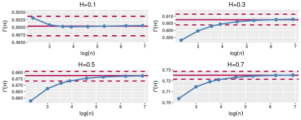
Figure 1: Convergence of $I^{n}(H)$ (blue) towards the benchmark MC value $I(H)$ (red) for different values of $(H,n)$ from Table 1. The dashed lines delimit the $90\%$ confidence interval of the Monte–Carlo simulation.

2.4 Connection to Riccati equations

The expression (2.13) is reminiscent of the formula obtained for finite dimensional Wishart processes in Bru (1991) and more generally that of linear quadratic diffusions, see Cheng and Scaillet (2007), suggesting a connection with infinite dimensional Riccati equations. Indeed, setting

$$\phi_{t,T} =-\frac{1}{2}\operatorname{Tr}\left(\log\left({\rm id}+2\sqrt{w}\mathbb{C}_{t}\sqrt{w}\right)\right),$$

$$\mathbb{\Psi}_{t,T} =-\sqrt{w}\left({\rm id}+2\sqrt{w}\mathbb{C}_{t}\sqrt{w}\right)^{-1}\sqrt{w},$$

it follows from Remark 2.4 that (2.13) can be rewritten as

$${\mathbb{E}}\left[\exp\left(-\int_{t}^{T}Z_{s}^{\top}wZ_{s}ds\right){\ \Big{|}\ }{\mathcal{F}}_{t}\right]=\exp\left({\phi}_{t,T}+\langle g_{t},\mathbb{\Psi}_{t,T}g_{t}\rangle_{L^{2}_{t}}\right),\quad t\leq{T}.$$ (2.21)

Since $t\to C_{t}(s,u)$ is absolutely continuous with density $\dot{C}_{t}(s,u)$ given by (2.4), one would expect $t\to{\mathbb{C}_{t}}$ to be strongly differentiable with derivative $\dot{\mathbb{C}}_{t}$ given by the integral operator

$$(\dot{\mathbb{C}}_{t}f)(s)=\int_{t}^{T}\dot{C}_{t}(s,u)f(u)du,\quad f\in L^{2}([0,T],{\mathbb{R}}^{N}),\quad s\leq T.$$ (2.23)

By taking the derivatives we get that $({\phi},\mathbb{\Psi})$ solves the following system of operator Riccati equations

$$\dot{{\phi}}_{t,T} =\operatorname{Tr}\left(\mathbb{\Psi}_{t,T}\dot{\mathbb{C}}_{t}\right), {{\phi}}_{T,T}=0,$$ (2.24)

$$\dot{\mathbb{\Psi}}_{t,T} =2\mathbb{\Psi}_{t,T}\sqrt{w}\dot{\mathbb{C}}_{t}\sqrt{w}\mathbb{\Psi}_{t,T}, {{\mathbb{\Psi}}_{T,T}=-w{\rm id}},$$ (2.25)

where $\dot{\mathbb{F}}_{t}$ denotes the derivative of $\mathbb{F}_{t}$ with respect to $t$.

This induces a system of Riccati equations for the kernels. To see this, we introduce the concept of resolvent. Fix $t\leq T$ and define the kernel

$$R^{w}_{t,T}(s,u)=\sum_{n\geq 1}\left(\frac{1}{1+2\lambda_{t,T}^{n}}-1\right)e_{t,T}^{n}(s)e_{t,T}^{n}(u)^{\top},\quad t\leq s,u\leq T.$$ (2.26)

It is straightforward to check, using (2.8), that for all $t\leq s,u\leq T$,

$$\!\!\!2\int_{t}^{T}R^{w}_{t,T}(s,z)C_{t}^{w}(z,u)dz=\!2\int_{t}^{T}C_{t}^{w}(s,z)R^{w}_{t,T}(z,u)dz=-R^{w}_{t,T}(s,u)-2C_{t}^{w}(s,u).\,\,\,\,\,\,$$ (2.27)

$R^{w}_{t,T}$ is called the resolvent kernel of $(-2C_{t}^{w})$ and the integral operator $\mathbb{R}^{w}_{t,T}$ induced by $R^{w}_{t,T}$ satisfies the relation

$$\mathbb{R}^{w}_{t,T}=({\rm id}+2\sqrt{w}\mathbb{C}_{t}\sqrt{w})^{-1}-{\rm id},$$ (2.28)

so that $\mathbb{\Psi}_{t,T}$ can be re-expressed in terms of the resolvent

$$\mathbb{\Psi}_{t,T}=-w{\rm id}-\sqrt{w}\mathbb{R}^{w}_{t,T}\sqrt{w}.$$

The next theorem, whose proof is postponed to Appendix C, establishes the representation of the Laplace transform together with the Riccati equations (2.24)-(2.25) in terms of the induced kernel

$$\Psi_{t,T}(ds,du)=-w\delta_{s=u}(ds,du)+\psi_{t,T}(s,u)dsdu,$$ (2.29)

where $\psi_{t,T}=-\sqrt{w}R^{w}_{t,T}\sqrt{w}$ is the density of $\Psi_{t,T}$ with respect to the Lebesgue measure. We recall the $\star$-product defined in (1.7).

Theorem 2.7.

Fix $w\in{\mathbb{S}}^{N}_{+}$ and $T>0$. Assume that the function $(s,u)\mapsto C_{t}(s,u)$ is continuous, for each $t\leq T$, such that

$$\sup_{t\leq T}\sup_{t\leq s,u\leq T}|C_{t}(s,u)|<\infty.$$ (2.30)

Assume that $t\mapsto\mathbb{C}_{t}$ is strongly differentiable on $[0,T]$ with derivative (2.23). Then,

$${\mathbb{E}}\left[\exp\left(-\int_{t}^{T}Z_{s}^{\top}wZ_{s}ds\right){\ \Big{|}\ }{\mathcal{F}}_{t}\right]=\exp\left({\phi}_{t,T}+\int_{(t,T]^{2}}g_{t}(s)^{\top}{\Psi}_{t,T}(ds,du)g_{t}(u)\right),\quad t\leq{T},$$ (2.31)

where $t\mapsto\Psi_{t,T}$ is given by (2.29) and $\phi_{t,T}$ by

$$\dot{\phi}_{t,T} =-\int_{(t,T]^{2}}\operatorname{tr}\left(\Psi_{t,T}(ds,du)K_{T}(u,t)K_{T}(s,t)^{\top}\right),\quad\phi_{T,T}=0.$$

In particular, $t\mapsto\Psi_{t,T}$ solves the Riccati equation with moving boundary

$$\dot{\psi}_{t,T} =2\Psi_{t,T}\star\dot{C}_{t}\star\Psi_{t,T}\quad\quad\mbox{on }(t,T]^{2}\quad a.e.,$$ (2.32)

$$\psi_{t,T}(t,\cdot) =\psi_{t,T}(\cdot,t)^{\top}=0\quad\,\;\;\;\,\;\,\,\,\,\mbox{on }\,[t,T]\,\,\quad a.e.$$ (2.33)

We note that, since $\psi_{t,T}(s,u)=0$ whenever $s\wedge u\leq t$, equation (2.32) is the compact form of

$$\dot{\psi}_{t,T}(s,u) =-2wK_{T}(s,t)K_{T}(u,t)^{\top}w$$

$$\quad-2wK_{T}(s,t)\int_{t}^{T}K_{T}(z,t)^{\top}\psi_{t,T}(z,u)dz$$

$$\quad-2\int_{t}^{T}\psi_{t,T}(s,z)K_{T}(z,t)dzK_{T}(u,t)^{\top}w$$

$$\quad-2\int_{t}^{T}\psi_{t,T}(s,z)K_{T}(z,t)dz\int_{t}^{T}K_{T}(z^{\prime},t)^{\top}\psi_{t,T}(z^{\prime},u)dz^{\prime},\quad t<s,u\leq T\;a.e.$$

and the expanded form of $\phi$ is given by

$$\dot{\phi}_{t,T} =\int_{t}^{T}\operatorname{tr}\left(wK_{T}(s,t)K_{T}(s,t)^{\top}\right)ds-\int_{t}^{T}\int_{t}^{T}\operatorname{tr}\left(\psi_{t,T}(s,u)K_{T}(u,t)K_{T}(s,t)^{\top}\right)dsdu.$$

Remark 2.8.

The Riccati equation (2.32) can be compared to the Bellman (1957) and Krein (1955) variation formula for Fredholm’s resolvent, see also Golberg (1973); Schumitzky (1968).

3 The Volterra Wishart process and its Laplace transforms

Fix $T>0$ and a filtered probability space $(\Omega,{\mathcal{F}},({\mathcal{F}}_{t})_{t\leq T},{\mathbb{P}})$ supporting a $d\times m$–matrix valued Brownian motion $W$. In this section, we consider the special case of the matrix-valued Volterra Gaussian process

$$X_{t} =g_{0}(t)+\int_{0}^{t}K(t,s)dW_{s},$$ (3.1)

where $g_{0}:[0,T]\to{\mathbb{R}}^{d\times m}$ is continuous and $K:[0,T]\to{\mathbb{R}}^{d\times d}$ is a $d\times d$–measurable kernel of Volterra type, that is $K(t,s)=0$ for $s>t$. Compared to (2.1), since the kernel $K$ is of Volterra type, the integration in (3.1) goes up to time $t$ rather than $T$.

Under the assumption

$$\sup_{t\leq T}\int_{0}^{T}|K(t,s)|^{2}ds<\infty\;\mbox{ and }\;\lim_{h\to 0}\int_{0}^{T}|K(u+h,s)-K(u,s)|^{2}ds=0,\;\;\;u\leq T,$$ (3.2)

the stochastic convolution

$$N_{t}=\int_{0}^{t}K(t,s)dW_{s},$$

is well defined as an Itô integral, for each $t\in[0,T]$. Furthermore, Itô’s isometry leads to

$${\mathbb{E}}\left[\left|N_{t}-N_{s}\right|^{2}\right]\leq 2\int_{s}^{t}|K(t,u)|^{2}du+2\int_{0}^{T}|K(t,u)-K(s,u)|^{2}du$$ (3.3)

which goes to $0$ as $s\to t$ showing that $N$ is mean-square continuous, and by virtue of Peszat and Zabczyk (2007, Proposition 3.21), the process $N$ admits a predictable version. Furthermore, by the Burkholder-Davis-Gundy inequality applied on the local martingale $\left(\int_{0}^{r}K(t,s)dW_{s}\right)_{r\in[0,t)}$, it holds that

$$\sup_{t\leq T}{\mathbb{E}}\left[\left|\int_{0}^{t}K(t,s)dW_{s}\right|^{p}\right]\leq c_{p,T}\left(\sup_{t\leq T}\int_{0}^{T}|K(t,s)|^{2}ds\right)^{p/2}<\infty,\quad p\geq 2,$$ (3.4)

where $c_{p,T}$ is a positive constant only depending on $T$ and $p$. Kernels satisfying (3.2) are known as Volterra kernels of continuous and bounded type in $L^{2}$ in the terminology of Gripenberg et al. (1990, Definitions 9.2.1, 9.5.1 and 9.5.2).

We now provide several kernels of interest that satisfy (3.2). In particular, we stress that (3.2) does not exclude a singularity of the kernel at $s=t$.

Example 3.1.

1. For $H\in(0,1)$, the fractional Brownian motion with covariance function (2.19) admits a Volterra representation of the form (3.1) on $[0,T]$ with the kernel

   $$K_{H}(t,s)=\frac{(t-s)^{H-1/2}}{\Gamma(H+\frac{1}{2})}\,{}_{2}F_{1}\left(H-\frac{1}{2};\frac{1}{2}-H;H+\frac{1}{2};1-\frac{t}{s}\right),\quad s\leq t,$$

   where ${}_{2}F_{1}$ is the Gauss hypergeometric integral, see Decreusefond and Ustunel (1999).

2. If $K$ is continuous on $[0,T]^{2}$, then (3.2) is satisfied by boundedness and the dominated convergence theorem. This is the case for instance for the Brownian Bridge $W^{T_{1}}$ conditioned to be equal to $W^{T_{1}}_{0}$ at a time $T_{1}$: for all $T<T_{1}$, $W^{T_{1}}$ admits the Volterra representation (3.1) on $[0,T]$ with the continuous kernel $K(t,s)=(T_{1}-t)/(T_{1}-s)$, for all $s,t\leq T$.

3. If $K_{1}$ an $K_{2}$ satisfy (3.2) then so does $K_{1}\star K_{2}$ by an application of Cauchy-Schwarz inequality.

4. Any convolution kernel of the form $K(t,s)=k(t-s)\mathbb{1}_{s\leq t}$ with $k\in L^{2}([0,T],{\mathbb{R}}^{d\times d})$ satisfies (3.2). Indeed, for any $t\leq T$,

   $$\int_{0}^{T}|K(t,s)|^{2}ds=\int_{0}^{t}|k(t-s)|^{2}ds=\int_{0}^{t}|k(s)|^{2}ds\leq\int_{0}^{T}|k(s)|^{2}ds,$$

   yielding the first part of (3.2). The second part follows from the $L^{2}$-continuity of $k$, see (Brezis, 2010, Lemma 4.3).

We denote the conditional expectation of $X$ by

$$g_{t}(s)={\mathbb{E}}\left[X_{s}|{\mathcal{F}}_{t}\right],\quad t\leq s\leq T,$$ (3.5)

which is well-defined thanks to (3.4). For each $t\geq 0$, we denote by $C_{t}$ the conditional covariance function of $X$ with respect to ${\mathcal{F}}_{t}$, that is

$$C_{t}(s,u)=\int_{t}^{s\wedge u}K(s,r)K(u,r)^{\top}dr,\quad t\leq s,u\leq T.$$ (3.6)

$C$ satisfies the assumption of Theorem 2.7 as shown in the next lemma. The expression of the strong derivative of $\bm{C}_{t}$ is given in terms of the density $\dot{C}_{t}$ of the kernel $C_{t}$ given by (2.4) under the following additional assumption on the kernel:

$$\sup_{t\leq T}\int_{0}^{T}|K(s,t)|^{2}ds<\infty.$$ (3.7)

Lemma 3.2.

Under (3.2), $(s,u)\mapsto C_{t}(s,u)$ is continuous, for all $t\leq T$ and (2.30) holds. Furthermore, under (3.7), $t\to\bm{C}_{t}$ is strongly differentiable on $[0,T]$ with derivative $\dot{\bm{C}}_{t}$ at $t\leq T$ given by the integral operator induced by the kernel $\bm{C_{t}}$ given by (2.4), that is

$$(\dot{\bm{C}}_{t}f)(s)=\int_{0}^{T}\dot{C}_{t}(s,u)f(u)du=\int_{t}^{T}\dot{C}_{t}(s,u)f(u)du,\quad f\in L^{2}\left([0,T],{\mathbb{R}}^{N}\right).\qquad$$ (3.8)

Proof.

First, it follows from (3.3) that the process $X$ is mean-square continuous, which implies the continuity of $(s,u)\mapsto C_{t}(s,u)$. Second, an application of the Cauchy-Schwarz inequality on (3.6) yields

$$|C_{t}(s,u)|^{2}\leq\left(\sup_{s^{\prime}\leq T}\int_{0}^{T}|K(s^{\prime},r)|^{2}dr\right)^{2}$$

which proves (2.30). Finally, to prove the differentiability statement, we fix $t\leq T$ and first observe that

$$\int_{0}^{T}\int_{0}^{T}|\dot{C}_{t}(s,u)|^{2}dsdu =\left(\int_{0}^{T}|K(s,t)|^{2}ds\right)^{2}$$

which is finite by virtue of (3.7). Whence, the kernel $\dot{C}_{t}$ belongs to $L^{2}\left([0,T]^{2},{\mathbb{R}}^{N\times N}\right)$ so that it induces a linear bounded integral operator $\dot{\mathbb{C}}_{t}$ from $L^{2}\left([0,T],{\mathbb{R}}^{N}\right)$ into istelf. We now prove that $r\mapsto\mathbb{C}_{r}$ is differentiable at $t$ with derivative given by $\dot{\mathbb{C}}_{t}$. For this, fix $f\in L^{2}\left([0,T],{\mathbb{R}}^{N}\right)$, $s\leq T$ and $h$ such that $t+h\leq T$. Using the fact that, for all $u,s\leq T$, $t\mapsto C_{t}(s,u)$ is absolutely continuous with density $\dot{C}_{t}(s,u)$, we get that

$$({\mathbb{C}}_{t+h}f)(s)-({\mathbb{C}}_{t}f)(s)-h(\dot{\mathbb{C}}_{t}f)(s)=\int_{0}^{T}\int_{t}^{t+h}\left(\dot{C}_{r}(s,u)-\dot{C}_{t}(s,u)\right)drf(u)du:=A(s).$$ (3.9)

We now bound the right hand side in $L^{2}\left([0,T],{\mathbb{R}}^{N}\right)$. Successive applications of the Cauchy-Schwarz inequality together with the Fubini-Tonelli theorem yield

$$\|A\|^{2}_{L^{2}} =\int_{0}^{T}\left(\int_{0}^{T}\int_{t}^{t+h}\left(\dot{C}_{r}(s,u)-\dot{C}_{t}(s,u)\right)drf(u)du\right)^{2}ds$$ (3.10)

$$\leq h\|f\|^{2}_{B}\int_{t}^{t+h}\int_{0}^{T}\int_{t}^{T}\left(\dot{C}_{r}(s,u)-\dot{C}_{t}(s,u)\right)^{2}dudsdr$$ (3.11)

Therefore,

$$\frac{1}{h}\|\mathbb{C}_{t+h}-\mathbb{C}_{t}-h\dot{\mathbb{C}}_{t}\|_{\rm{op}}\leq\int_{t}^{t+h}\int_{0}^{T}\int_{0}^{T}\left(\dot{C}_{r}(s,u)-\dot{C}_{t}(s,u)\right)^{2}dudsdr.$$ (3.12)

The right hand side goes to $0$ by virtue of (3.7), which ends the proof. ∎

3.1 A first representation

By construction the process $XX^{\top}$ is ${\mathbb{S}}^{d}_{+}$–valued and its Laplace transforms can be deduced from Theorems  2.2 and 2.7. Indeed, using the vectorization operator $\operatorname{vec}$, which stacks the column of a $d\times m$–matrix $A$ one underneath another in a vector of dimension $N=dm$, see Appendix B, the study of the matrix valued process $X$ reduces to that of the ${\mathbb{R}}^{dm}$-valued Gaussian process $Z=\operatorname{vec}(X)$ as done in Section 2.

The following theorem represents the main result of the paper.

Theorem 3.3.

Let $X$ be the $d\times m$–matrix valued process defined in (3.1) for some Volterra kernel $K$ satisfying (3.2) and (3.7). Fix $t\leq T$. For any $u\in{\mathbb{S}}^{d}_{+}$,

$$\!\!\!{\mathbb{E}}\left[\exp\left(-\operatorname{tr}\left(uX_{T}X_{T}^{\top}\right)\right){\ \Big{|}\ }{\mathcal{F}}_{t}\right]=\frac{\exp\left(-\operatorname{tr}\left(u\left(I_{d}+2C_{t}(T,T)u\right)^{-1}g_{t}(T)g_{t}(T)^{\top}\right)\right)}{\det\left(I_{d}+2C_{t}(T,T)u\right)^{m/2}}.\;\,\;\;$$ (3.13)

For any $w\in{\mathbb{S}}^{d}_{+}$, the Laplace transform

$$\mathcal{L}_{t,T}(w)={\mathbb{E}}\left[\exp\left(-\int_{t}^{T}\operatorname{tr}\left(wX_{s}X_{s}^{\top}\right)ds\right){\ \Big{|}\ }{\mathcal{F}}_{t}\right],$$

is given by

$$\mathcal{L}_{t,T}(w)=\exp\left(\phi_{t,T}+\int_{(t,T]^{2}}\operatorname{tr}\left(g_{t}(s)^{\top}\Psi_{t,T}(ds,du)g_{t}(u)\right)\right),$$ (3.14)

where $(\phi,\Psi)$ are defined by

$$\dot{\phi}_{t,T} =-m\int_{(t,T]^{2}}\operatorname{tr}\left(\Psi_{t,T}(ds,du)K(u,t)K(s,t)^{\top}\right),\quad\phi_{T,T}=0,$$ (3.15)

$$\Psi_{t,T}(ds,du) =-w\delta_{\{s=u\}}(ds,du)-\sqrt{w}R^{w}_{t,T}(s,u)\sqrt{w}dsdu,\quad\mbox{on}\quad[t,T],$$ (3.16)

where $R^{w}_{t,T}$ is the $d\times d$–matrix valued resolvent of $(-2\sqrt{w}C_{t}\sqrt{w})$, with $C_{t}$ the conditional covariance function (3.6) and $g_{t}$ the conditional mean given by (3.5). In particular, $t\mapsto\Psi_{t,T}$ solves the Riccati equation with moving boundary

$$\dot{\psi}_{t,T} =2\Psi_{t,T}\star\dot{C}_{t}\star\Psi_{t,T}\quad\mbox{on }(t,T]^{2}\quad a.e.,$$ (3.17)

$$\psi_{t,T}(t,\cdot) =\psi_{t,T}(\cdot,t)^{\top}=0\quad\,\;\,\,\,\,\mbox{on }\,[t,T]\,\,\quad a.e.,$$ (3.18)

where $\psi_{t,T}(s,u)=\sqrt{w}R^{w}_{t,T}(s,u)\sqrt{w}$.

Proof.

Setting $Z=\operatorname{vec}(X)$ and $\bm{W}=\operatorname{vec}(W)$, an application of the vectorization operator $\operatorname{vec}$ on both sides of the $d\times m$–matrix valued equation (3.1) yields the $N:=dm$ dimensional vector valued Gaussian process

$$Z_{s}=\operatorname{vec}\left({g_{0}}(s)\right)+\int_{0}^{s}\mathcal{K}(s,u)d\bm{W}_{u}.$$ (3.19)

where $\mathcal{K}$ is the ${\mathbb{R}}^{N\times N}$ kernel

$$\mathcal{K}:(s,u)\mapsto(I_{m}\otimes K(s,u))$$

coming from the relation (B.1), with $\otimes$ the Kronecker product. Whence, the conditional mean and covariance functions of $Z$ are given respectively by $\operatorname{vec}(g_{t})$ and

$${\mathcal{C}}_{t}(s,u)=(I_{m}\otimes C_{t}(s,u)),\quad u,s\leq T.$$ (3.20)

In addition, due to (B.2),

$$\operatorname{tr}(wXX^{\top})=Z^{\top}(I_{m}\otimes w)Z,\quad w\in{\mathbb{S}}^{N}.$$ (3.21)

$\bullet$ We first prove (3.13). Fix $t\leq T$ and $u\in{\mathbb{S}}^{d}_{+}$. An application of Theorem 2.2 yields

$${\mathbb{E}}\left[\exp\left(-Z_{T}^{\top}(I_{m}\otimes u)Z_{T}\right){\ \Big{|}\ }{\mathcal{F}}_{t}\right]=\frac{\exp\left(-H_{t}(T)\right)}{\det\left(I_{N}+2\mathcal{C}_{t}(T,T)(I_{m}\otimes u)\right)^{1/2}},$$ (3.22)

with

$$H_{t}(T) =\operatorname{vec}(g_{t}(T))^{\top}(I_{m}\otimes u)\left(I_{N}+2\mathcal{C}_{t}(T,T)(I_{m}\otimes u)\right)^{-1}\operatorname{vec}(g_{t}(T)).$$ (3.23)

We observe that by (3.20) and successive applications of the product rule (B.3)

$$\left(I_{N}+2\mathcal{C}_{t}(T,T)(I_{m}\otimes u)\right)^{-1} =\left((I_{m}\otimes I_{d})+2(I_{m}\otimes C_{t}(T,T))(I_{m}\otimes u)\right)^{-1}$$

$$=\left(I_{m}\otimes\left(I_{d}+2C_{t}(T,T)u\right)\right)^{-1}$$

$$=\left(I_{m}\otimes\left(I_{d}+2C_{t}(T,T)u\right)^{-1}\right)$$

where the last equality follows from (B.5). Another application of (B.3) combined with (B.2) yields that

$$H_{t}(T)=\operatorname{tr}\left(u\left(I_{d}+2C_{t}(T,T)u\right)^{-1}g_{t}(T)g_{t}(T)^{\top}\right).$$ (3.24)

Similarly,

$$\det\left(I_{N}+2\mathcal{C}_{t}(T,T)(I_{m}\otimes u)\right) =\det\left(I_{m}\otimes\left(I_{d}+2C_{t}(T,T)u\right)\right)$$ (3.25)

$$=\det\left(I_{m}\otimes\left(I_{d}+2C_{t}(T,T)u\right)\right)$$ (3.26)

$$=\det\left(I_{d}+2C_{t}(T,T)u\right)^{m}$$ (3.27)

where we used (B.6) for the last identity. Combining the above proves (3.13).
$\bullet$ We now prove (3.14). Fix $t\leq T$ and $w\in{\mathbb{S}}^{d}_{+}$. An application of Theorem 2.7, justified by Lemma 3.2, yields that

$$\mathcal{L}_{t,T}(w)=\exp\left(\phi_{t,T}+\int_{(t,T]^{2}}\operatorname{vec}(g_{t}(s))^{\top}\widetilde{\Psi}_{t,T}(ds,du)\operatorname{vec}(g_{t}(u))\right),$$ (3.28)

where

$$\dot{\phi}_{t,T} =-\int_{(t,T]^{2}}\operatorname{tr}\left(\widetilde{\Psi}_{t,T}(ds,du)\mathcal{K}(u,t)\mathcal{K}(s,t)^{\top}\right),\quad\phi_{T,T}=0,$$ (3.29)

$$\widetilde{\Psi}_{t,T}(ds,du) =-(I_{m}\otimes w)\delta_{s=u}(ds,du)-(I_{m}\otimes\sqrt{w})\widetilde{\mathcal{R}}^{w}_{t,T}(s,u)(I_{m}\otimes\sqrt{w})dsdu,$$

and $\widetilde{\mathcal{R}}^{w}_{t,T}$ is the resolvent of $2{\mathcal{C}}^{w}_{t}(s,u)$. The claimed expressions now follows provided we prove that

$$\widetilde{\mathcal{R}}^{w}_{t,T}=\left(I_{m}\otimes R^{w}_{t,T}\right),$$ (3.30)

where $R^{w}_{t,T}$ is the resolvent kernel of $2{C}^{w}_{t}(s,u)$. Indeed, if this is the case, then, using the the product rule (B.3) we get that

$$\widetilde{\Psi}_{t,T}=\left(I_{m}\otimes\Psi_{t,T}\right),$$ (3.31)

where $\Psi_{t,T}$ is given by (3.16), so that, by (B.2),

$$\operatorname{vec}(g_{t}(s))^{\top}\widetilde{\Psi}_{t,T}(ds,du)\operatorname{vec}(g_{t}(u))=\operatorname{tr}\left(g_{t}(s)^{\top}{\Psi}_{t,T}(ds,du)g_{t}(u)\right).$$

Plugging (3.31) back in (3.29) and using the identity (B.4) yields (3.15). Combining the above shows that (3.28) is equal to (3.14). We now prove (3.30). For this, we define ${\mathcal{R}}^{w}_{t,T}=\left(I_{m}\otimes R^{w}_{t,T}\right).$ Then, it follows from the resolvent equation (2.27) of $R^{w}_{t,T}$ and the product rule (B.3) that ${\mathcal{R}}^{w}_{t,T}$ solves

$${\mathcal{R}}^{w}_{t,T}=-2\mathcal{C}_{t}-2{\mathcal{R}}^{w}_{t,T}\star\mathcal{C}_{t},\quad{\mathcal{R}}^{w}_{t,T}\star\mathcal{C}_{t}=\mathcal{C}_{t}\star{\mathcal{R}}^{w}_{t,T},$$

showing that ${\mathcal{R}}^{w}_{t,T}$ is a resolvent of $(-2\mathcal{C}_{t})$. By uniqueness of the resolvent, see Gripenberg et al. (1990, Lemma 9.3.3), (3.30) holds.
$\bullet$ Finally, the Riccati equations (3.17)–(3.18) follow along the same lines by invoking Theorem 2.7. ∎

Remark 3.4.

Proposition 2.6 can be applied to the vectorized Gaussian process $Z=\operatorname{vec}(X)$ given by (3.19) to get an approximation formula for

$${\mathbb{E}}\left[\exp\left(-\int_{t}^{T}\operatorname{tr}\left(wX_{s}X_{s}^{\top}\right)ds\right){\ \Big{|}\ }{\mathcal{F}}_{t}\right]={\mathbb{E}}\left[\exp\left(-\int_{t}^{T}\operatorname{tr}\left(Z_{s}^{\top}(I_{m}\otimes w)Z_{s}\right)ds\right){\ \Big{|}\ }{\mathcal{F}}_{t}\right].$$

3.2 A second representation for certain convolution kernels

The aim of this section is to link the Volterra Wishart distribution with conventional linear-quadratic processes (Chen et al., 2004; Cheng and Scaillet, 2007) for the special case of convolution kernels:

$$K(t,s)=k(t-s)\bm{1}_{s\leq t}\quad\mbox{ such that }\quad k(t)=\int_{{\mathbb{R}}_{+}}e^{-xt}\mu(dx),\quad t>0,$$ (3.32)

where $\mu$ is a $d\times m$–measure of locally bounded variation satisfying

$$\int_{{\mathbb{R}}_{+}}\left(1\wedge x^{-1/2}\right)|\mu|(dx)<\infty,$$ (3.33)

and $|\mu|$ is the total variation of the measure, as defined in Gripenberg et al. (1990, Definition 3.5.1). The condition (3.33) ensures that $k$ is locally square integrable, see Abi Jaber et al. (2019b, Lemma A.1). This is inspired by the approach initiated in Carmona et al. (2000) and generalized to stochastic Volterra equations in Abi Jaber and El Euch (2019b); Cuchiero and Teichmann (2019); Harms and Stefanovits (2019).

Several kernels of interest satisfy (3.32)-(3.33) such as weighted sums of exponentials and the Riemann-Liouville fractional kernel $K_{RL}(t)=\frac{t^{H-1/2}}{\Gamma(H+1/2)},$ for $H\in(0,1/2)$. We refer to Abi Jaber et al. (2019b, Example 2.2) for more examples.

A straightforward application of stochastic Fubini’s theorem provides the representation of $(X_{t},g_{t})_{t\geq 0}$ in terms of $\mu$ and the possibly infinite system of $d\times m$-matrix-valued Ornstein-Uhlenbeck processes

$$Y_{t}(x)=\int_{0}^{t}e^{-x(t-s)}dW_{s},\quad t\geq 0,\quad x\in{\mathbb{R}}_{+},$$

see for instance Abi Jaber et al. (2019b, Theorem 2.3).

Lemma 3.5.

Assume that $K$ is of the form (3.32) with $\mu$ satisfying (3.33), then

$$X_{t} =g_{0}(t)+\int_{{\mathbb{R}}_{+}}\mu(dx)Y_{t}(x), t\leq T,$$

$$g_{t}(s) =g_{0}(s)+\int_{{\mathbb{R}}_{+}}e^{-x(s-t)}\mu(dx)Y_{t}(x), t\leq s\leq T.$$

Combined with (3.14), we get an exponentially quadratic representations of the characteristic function of $XX^{\top}$ in terms of the process $Y$.

Theorem 3.6.

Assume that $K$ is of the form (3.32) with $\mu$ satisfying (3.33) and fix $w\in{\mathbb{S}}^{d}_{+}$. Then,

$$\mathcal{L}_{t,T}(w)=\exp\Bigg{(}\Theta_{t,T} +2\operatorname{tr}\left(\int_{{\mathbb{R}}_{+}}\Lambda_{t,T}(x)^{\top}\mu(dx)Y_{t}(x)\right)$$ (3.34)

$$\quad\quad+\operatorname{tr}\left(\int_{{\mathbb{R}}_{+}^{2}}Y_{t}(x)^{\top}\mu(dx)^{\top}\Gamma_{t,T}(x,y)\mu(dy)Y_{t}(y)\right)\Bigg{)},$$ (3.35)

where $t\mapsto(\Theta_{t,T},\Lambda_{t,T},\Gamma_{t,T})$ are given by

$$\Theta_{t,T} =\int_{(t,T]^{2}}\operatorname{tr}\left(g_{0}(s)^{\top}\Psi_{t,T}(ds,du)g_{0}(s)\right)+\phi_{t,T},$$ (3.36)

$$\Lambda_{t,T}(x) =\int_{(t,T]^{2}}e^{-x(s-t)}\Psi_{t,T}(ds,du)g_{0}(u),$$ (3.37)

$$\Gamma_{t,T}(x,y) =\int_{(t,T]^{2}}e^{-x(s-t)}\Psi_{t,T}(ds,du)e^{-y(u-t)},$$ (3.38)

with $(\phi,\Psi)$ as in (3.15)-(3.16).

A direct differentiation of $(\Theta,\Lambda,\Gamma)$ combined with the Riccati equations (3.17)–(3.18) for $(\phi,\Psi)$ yield a system of Riccati equation for $(\Theta,\Lambda,\Gamma)$.

Proposition 3.7.

The functions $t\mapsto(\Theta_{t,T},\Lambda_{t,T},\Gamma_{t,T})$ given by (3.36), (3.37) and (3.38) solve the system of backward Riccati equations

$$\dot{\Theta}_{t,T} =-\mathcal{R}_{0}(t,\Lambda_{t,T},\Gamma_{t,T}), \Theta_{T,T}=0,$$ (3.39)

$$\dot{\Lambda}_{t,T}(x) =x\Lambda_{t,T}(x)-\mathcal{R}_{1}(t,\Lambda_{t,T},\Gamma_{t,T})(x), \Lambda_{T,T}(x)=0,$$ (3.40)

$$\dot{\Gamma}_{t,T}(x,y) =(x+y)\Gamma_{t,T}(x,y)-\mathcal{R}_{2}(\Gamma_{t,T})(x,y), \Gamma_{T,T}(x,y)=0,$$ (3.41)

where

$$\mathcal{R}_{0}(t,\Lambda,\Gamma) =-\operatorname{tr}\left(g_{0}(t)^{\top}wg_{0}(t)\right)+m\operatorname{tr}\left(\int_{{\mathbb{R}}_{+}^{2}}\Gamma(x,y)\mu(dy)\mu(dx)^{\top}\right)$$

$$\quad\;+2\operatorname{tr}\left(\left(\int_{{\mathbb{R}}_{+}}\Lambda(x)^{\top}\mu(dx)\right)\left(\int_{{\mathbb{R}}_{+}}\Lambda(y)^{\top}\mu(dy)\right)^{\top}\right),$$

$$\mathcal{R}_{1}(t,\Lambda,\Gamma)(x) =-wg_{0}(t)+2\left(\int_{{\mathbb{R}}_{+}}\Gamma(x,x^{\prime})\mu(dy)\right)\left(\int_{{\mathbb{R}}_{+}}\Lambda(y)^{\top}\mu(dy)\right)^{\top},$$

$$\mathcal{R}_{2}(\Gamma)(x,y) =-w+2\left(\int_{{\mathbb{R}}_{+}}\Gamma(x,x^{\prime})\mu(dx^{\prime})\right)\left(\int_{{\mathbb{R}}_{+}}\Gamma(y,y^{\prime})\mu(dy^{\prime})\right)^{\top}.$$

Similar Riccati equations to that of $\Gamma$ have appeared in the literature when dealing with convolution kernels of the form (3.32) in the presence of a quadratic structure, see Abi Jaber et al. (2019b, Theorem 3.7), Alfonsi and Schied (2013, Theorem 1), Harms and Stefanovits (2019, Lemma 5.4), Cuchiero and Teichmann (2019, Corollary 6.1). A general existence and uniqueness result for more general equations has been recently obtained in Abi Jaber et al. (2019c).

Remark 3.8.

The expression (3.35) can be re-written in the following compact form

$$\mathcal{L}_{t,T}(w)=\exp\left(\Theta_{t,T}+2\langle\Lambda_{t,T},Y_{t}\rangle_{\mu}+\langle Y_{t},\mathbb{\Gamma}_{t,T}Y_{t}\rangle_{\mu}\right).$$

where $\mathbb{\Gamma}_{t,T}$ is the integral operator acting on $L^{1}(\mu,{\mathbb{R}}^{d\times m})$ induced by the kernel ${\Gamma}_{t,T}$:

$$(\mathbb{\Gamma}_{t,T}f)(x)=\int_{{\mathbb{R}}_{+}}{\Gamma}_{t,T}(x,y)\mu(dy)f(y),\quad f\in L^{1}(\mu,{\mathbb{R}}^{d\times m})$$

and $\langle\cdot,\cdot\rangle_{\mu}$ is the dual pairing

$$\langle f,g\rangle_{\mu}=\operatorname{tr}\left(\int_{{\mathbb{R}}_{+}}f(x)^{\top}\mu(dx)^{\top}g(x)\right),\quad(f,g)\in L^{1}(\mu,{\mathbb{R}}^{d\times m})\times L^{\infty}(\mu^{\top},{\mathbb{R}}^{d\times m}).$$

We end this subsection with two examples establishing the connection with conventional quadratic models.

Example 3.9.

Fix $\Sigma\in{\mathbb{R}}^{d\times d}$. For the constant case $k\equiv\Sigma$ we have $\mu({dx})=\Sigma\delta_{0}(dx)$, $\operatorname{supp}\mu=\{0\}$ and $Y_{t}(0)=W_{t}\in{\mathbb{R}}^{d\times m}$. For $g_{0}(t)\equiv 0$, $\Lambda\equiv 0$ and (3.39) and (3.41) read

$$\dot{\Theta}_{t,T} =-m\operatorname{tr}\left(\Gamma_{t,T}(0,0)\Sigma\Sigma^{\top}\right), \Theta_{T,T}=0,$$

$$\dot{\Gamma}_{t,T}(0,0) =w-2\Gamma_{t,T}(0,0)\Sigma\Sigma^{\top}\Gamma_{t,T}(0,0), \Gamma_{T,T}(0,0)=0.$$

These are precisely the conventional backward matrix Riccati equations encountered for conventional Wishart processes, see Alfonsi (2015, Equation (5.15)). In this case, we recover the well-known Markovian expression for the conditional Laplace transform (3.35):

$${\mathbb{E}}\left[\exp\left(\int_{t}^{T}\operatorname{tr}\left(-wW_{s}W_{s}^{\top}\right)ds\right){\ \Big{|}\ }{\mathcal{F}}_{t}\right]=\exp\left(\Theta_{t,T}+\operatorname{tr}\left(\Gamma_{t,T}(0,0)W_{t}W_{t}^{\top}\right)\right).$$

Example 3.10.

Fix $n\geq 1$, $x^{n}_{i}\in{\mathbb{R}}_{+}$ and $c^{n}_{i}\in{\mathbb{R}}^{d\times d}$, $i=1,\ldots,n$. Consider the kernel

$$k^{n}(t)=\sum_{i=1}^{n}c^{n}_{i}e^{-x^{n}_{i}t},\quad t\geq 0,$$ (3.42)

which corresponds to the measure $\mu^{n}(dx)=\sum_{i=1}^{n}c^{n}_{i}\delta_{x^{n}_{i}}(dx)$. The system of Riccati equations (3.39), (3.40) (3.41) is reduced to a system of finite dimensional matrix Riccati equations for with values in ${\mathbb{R}}\times{\mathbb{R}}^{nd\times m}\times{\mathbb{R}}^{nd\times nd}$ given by:

$$\dot{\Theta}_{t,T}^{n} =\operatorname{tr}\left(g_{0}(t)^{\top}wg_{0}(t)\right)-m\operatorname{tr}\left(\Gamma^{n}_{t,T}C^{n}\right)-2\operatorname{tr}\left(\Lambda^{n\top}_{t,T}C^{n}\Lambda^{n}_{t,T}\right), \!\!\!\!\!\!\!\!\!\Theta^{n}_{T,T}=0,$$ (3.43)

$$\dot{\Lambda}^{n}_{t,T} =D^{n}_{t}+B^{n}\Lambda^{n}_{t,T}-2\Gamma^{n}_{t,T}C^{n}\Lambda^{n}_{t,T}, \!\!\!\!\!\!\!\!\!\Lambda^{n}_{T,T}=0,$$ (3.44)

$$\dot{\Gamma}^{n}_{t,T} =A^{n}+B^{n}\Gamma^{n}_{t,T}+\Gamma^{n}_{t,T}B^{n\top}-2\Gamma^{n}_{t,T}C^{n}\Gamma^{n}_{t,T}, \!\!\!\!\!\!\!\!\!\Gamma^{n}_{T,T}=0,$$ (3.45)

where for all $r=1,\ldots,m$ $i,j,=1,\ldots,n$ and $k,l=1,\ldots,d$, $p=(i-1)d+k,q=(j-1)d+l,$

$$(D^{n}_{t})^{pr} =(wg_{0}(t))^{kr}, (\Lambda^{n}_{t,T})^{pr}=\Lambda_{t,T}(x_{i})^{kr},$$ (3.46)

$$(C^{n})^{pq} =(c_{i}^{n}c_{j}^{n\top})^{kl}, (\Gamma^{n}_{t,T})^{pq}=\Gamma_{t,T}(x_{i}^{n},x_{j}^{n})^{kl},$$ (3.47)

and $A^{n}$ and $B^{n}$ are the $nd\times nd$ defined by

$$A^{n}=(\mathbbm{1}_{n}\otimes w),\quad B^{n}=(\operatorname{diag}(x_{1}^{n},\ldots,x^{n}_{n})\otimes I_{d})$$ (3.48)

with $\mathbbm{1}_{n}$ the $n\times n$ matrix with all components equal to $1$. The Riccati equation (3.45) can be linearized by doubling the dimension and its solution is given explicitly by

$$\Gamma^{n}_{t,T}=G_{2}(T-t)G_{4}(T-t)^{-1},\quad t\leq T,$$

where

$$\left(\begin{matrix}G_{1}(t)&G_{2}(t)\\ G_{3}(t)&G_{4}(t)\\ \end{matrix}\right)=\exp\left(t\left(\begin{matrix}-B^{n}&-A^{n}\\ -2C^{n}&B^{n}\\ \end{matrix}\right)\right),\quad t\leq T,$$ (3.49)

see Levin (1959). Furthermore, we recover the well-known Markovian expression for the conditional Laplace transform (3.35):

$$\mathcal{L}_{t,T}^{n}(w)=\exp\left(\Theta^{n}_{t,T}+2\operatorname{tr}\left(\Lambda^{n\top}_{t,T}\widetilde{Y}_{t}^{n}\right)+\operatorname{tr}\left(\Gamma^{n}_{t,T}\widetilde{Y}_{t}^{n}\widetilde{Y}_{t}^{n\top}\right)\right),$$ (3.50)

where

$$(\widetilde{Y}^{n}_{t})^{pr}=(c_{i}^{n}Y_{t}(x_{i}^{n}))^{kr},$$ (3.51)

$p=(i-1)d+k$, for each $i=1,\ldots,n$, $k=1,\ldots,d$, $r=1,\ldots,m$.

The previous example shows that Volterra Wishart processes can be seen as a superposition of possibly infinitely many conventional linear-quadratic processes in the sense of Chen et al. (2004); Cheng and Scaillet (2007). This idea is used to build another approximation procedure in the next subsection.

3.3 Another approximation procedure

An application of the Burkholder-Davis-Gundy inequality yields the following stability result for the sequence

$$X^{n}_{t} =g^{n}_{0}(t)+\int_{0}^{t}k^{n}(t-s)dW_{s},\quad n\geq 1,$$

where $g_{0}^{n}:[0,T]\to{\mathbb{R}}^{d\times m}$ and $k^{n}\in L^{2}([0,T],{\mathbb{R}}^{d\times d})$, for each $n\geq 1$.

Lemma 3.11.

Fix $k\in L^{2}([0,T],{\mathbb{R}}^{d\times d})$ and $g_{0}:[0,T]\to{\mathbb{R}}^{d\times m}$ measurable and bounded. If

$$\int_{0}^{T}|k^{n}(s)-k(s)|^{2}ds\to 0\quad\mbox{and}\quad\sup_{t\leq T}|g_{0}^{n}(t)-g_{0}(t)|\to 0,\quad\mbox{as \, $n\to\infty$},$$ (3.52)

then,

$$\sup_{t\leq T}{\mathbb{E}}\left[\left|X^{n}_{t}-X_{t}\right|^{p}\right]\to 0,\quad\mbox{as \, $n\to\infty$},\quad p\geq 2.$$ (3.53)

Combined with Example 3.10, we obtain another approximation scheme for the Laplace transform based on finite-dimensional matrix Riccati equations (compare with Remark 3.4).

Proposition 3.12.

Fix $w\in{\mathbb{S}}^{d}_{+}$ and $t\leq T$. For each $n$, let $k^{n}$ be as in (3.42) for some $x^{n}_{i}\in{\mathbb{R}}_{+}$ and $c^{n}_{i}\in{\mathbb{R}}^{d\times d}$. Assume that (3.52) holds. Then,

$$\mathcal{L}_{t,T}(w)=\lim_{n\to\infty}\exp\left(\Theta^{n}_{t,T}+2\operatorname{tr}\left(\Lambda^{n\top}_{t,T}\widetilde{Y}_{t}^{n}\right)+\operatorname{tr}\left(\Gamma^{n}_{t,T}\widetilde{Y}_{t}^{n}\widetilde{Y}_{t}^{n\top}\right)\right)$$ (3.54)

where $(\Theta^{n},\Lambda^{n},\Gamma^{n})$ solve (3.43), (3.44) and (3.45) and $\widetilde{Y}^{n}$ is given by (3.51).

Proof.

Fix $t\leq s\leq T$. Writing $X^{n\top}_{s}wX^{n}_{s}-X_{s}^{\top}wX_{s}=(X^{n}_{s}+X_{s})^{\top}w(X^{n}_{s}-X_{s})$, we get by the Cauchy-Schwarz inequality that

$${\mathbb{E}}\left[\left|\int_{t}^{T}(X^{n\top}_{s}wX^{n}_{s}-X_{s}^{\top}wX_{s})ds\right|^{2}\right]\leq c\sup_{s\leq T}\left({\mathbb{E}}\left[|X_{s}|^{2}\right]+{\mathbb{E}}\left[|X^{n}_{s}|^{2}\right]\right)\sup_{s\leq T}{\mathbb{E}}\left[|X^{n}_{s}-X_{s}|^{2}\right],$$

for some constant $c$ independent of $n$. It follows from Lemma 3.11 that $(\sup_{s\leq T}{\mathbb{E}}\left[|X^{n}_{s}|^{2}\right])_{n\geq 1}$ is uniformly bounded in $n$, so that the right hand side converges to $0$ as $n\to\infty$. Whence, $\int_{t}^{T}X^{n\top}_{s}wX^{n}_{s}ds\to\int_{t}^{T}X^{\top}_{s}wX_{s}ds$ a.s. along a subsequence and the claimed convergence follows from the dominated convergence theorem combined with (3.50). ∎

For $d=m=1$ and $k$ of the form (3.32) for some measure $\mu$, for suitable partitions $(\eta^{n}_{i})_{0\leq i\leq n}$ of ${\mathbb{R}}_{+}$, the choice

$$c^{n}_{i}=\int_{\eta_{i-1}^{n}}^{\eta_{i}^{n}}\mu(dx)\quad\mbox{and}\quad x^{n}_{i}=\frac{1}{c^{n}_{i}}\int_{\eta_{i-1}^{n}}^{\eta_{i}^{n}}x\mu(dx),\quad i=1,\ldots,n,$$

ensures the $L^{2}$-convergence of the kernels $k^{n}$ in (3.42), we refer to Abi Jaber (2019); Abi Jaber and El Euch (2019a) for such constructions, see also Harms (2019) for other choices of quadratures and for a detailed study of strong convergence rates.

4 Applications

4.1 Bond pricing in quadratic Volterra short rate models with default risk

We consider a quadratic short rate model of the form

$$r_{t}=\operatorname{tr}\left(X_{t}^{\top}QX_{t}\right)+\xi(t),\quad t\leq T,$$

where $X$ is the $d\times m$ Volterra process as in (3.1), $Q\in{\mathbb{S}}^{d}_{+}$ and $\xi:[0,T]\to{\mathbb{R}}$ is an input curve used to match today’s yield curve and/or control the negativity level of the short rate. The model replicates the asymmetrical distribution of interest rates, allows for rich auto-correlation structures, and the possibility to account for long range dependence, see for instance Benth and Rohde (2018); Corcuera et al. (2013).

An application of Theorem 3.3 yields the price $P(\cdot,T)$ of a zero-coupon bond with maturity $T$:

$$P(t,T) ={\mathbb{E}}\left[\exp\left(-\int_{t}^{T}r_{s}ds\right){\ \Big{|}\ }{\mathcal{F}}_{t}\right]=\exp\left(-\int_{t}^{T}\xi(s)ds\right)\mathcal{L}_{t,T}(Q),\quad t\leq T,$$

where $\mathcal{L}$ is given by (3.14).

One can also add a spread by considering the stochastic process

$$\lambda_{t}=\operatorname{tr}\left(X_{t}^{\top}\widetilde{Q}X_{t}\right)+\widetilde{\xi}(t),\quad t\leq T,$$

for some $\widetilde{Q}\in{\mathbb{S}}^{d}_{+}$ and $\widetilde{\xi}:[0,T]\to{\mathbb{R}}_{+}$ bounded function. By definition the spread is nonnegative, correlated to the short rate with a possible long range dependence or roughness. The introduction of $\lambda$ can serve in two ways. Either in a multiple curve modeling framework, to add a risky curve on top of the non-risk one with instantaneous rate $r+\lambda$ or to model default time. In the latter case, $\lambda$ would correspond to the instantaneous intensity of a Poisson process $N$ such that the default time $\tau$ is defined as the first jump time of $N$. In both cases, we denote by $\widetilde{P}(\cdot,T)$ the price of the risky curve or the price of a defaultable bond paying $\mathbb{1}_{\tau\leq T}$ at maturity $T$. Then, the price is given by

$$\widetilde{P}(t,T) ={\mathbb{E}}\left[\exp\left(-\int_{t}^{T}(r_{s}+\lambda_{s})ds\right){\ \Big{|}\ }{\mathcal{F}}_{t}\right]$$

$$=\exp\left(-\int_{t}^{T}(\xi(s)+\widetilde{\xi}(s))ds\right)\mathcal{L}_{t,T}(Q+\widetilde{Q}),$$

for all $t\leq T$, we refer to Lando (1998) for more details on the derivation of the defaultable bond price.

In practice, Proposition 3.4 can be used to approximate $\mathcal{L}_{t,T}$, and consequently $P$ and $\widetilde{P}$, see also Remark 3.4. For kernels of the form (3.32) the approximation results of Section 3.3 also apply.

4.2 Pricing options on volatility/variance for basket products in Volterra Wishart covariance models

We consider $d\geq 1$ risky assets $S=(S^{1},\ldots,S^{d})$ such that the instantaneous realized covariance is given by

$$d\langle\log S\rangle_{t}=X_{t}X_{t}^{\top}dt$$ (4.1)

where $X$ is the $d\times m$ process as in (3.1). The following specifications for the dynamics of $S$ fall into this framework.

Example 4.1.

1. The Volterra Wishart covariance model for $d=m$:

   $$dS_{t} =\operatorname{diag}(S_{t})X_{t}dB_{t},\quad S_{0}\in{\mathbb{R}}^{d}_{+}$$

   $$X_{t} =g_{0}(t)+\int_{0}^{t}K(t,s)dW_{s},$$

   with $g_{0}:[0,T]\to{\mathbb{R}}^{d\times d}$, a suitable measurable kernel $K:[0,T]^{2}\to{\mathbb{R}}^{d\times d}$, a $d\times d$ Brownian motion $W$ and

   $$B^{j}=\operatorname{tr}\left(W_{j}\rho_{j}^{\top}\right)+\sqrt{1-\operatorname{tr}\left(\rho_{j}\rho_{j}^{\top}\right)}\,W^{\perp,j},\quad j=1,\ldots,d,$$ (4.2)

   for some $\rho_{j}\in{\mathbb{R}}^{d\times m}$ such that $\operatorname{tr}\left(\rho_{j}\rho_{j}^{\top}\right)\leq 1$, for $j=1,\ldots,n$, where $W^{\perp}$ is a $d$–dimensional Brownian motion independent of $W$.

2. The Volterra Stein-Stein model when $d=m=1$:

   $$dS_{t} =S_{t}X_{t}dB_{t},\quad S_{0}>0,$$

   $$X_{t} =g_{0}(t)+\int_{0}^{t}K(t,s)dW_{s},\quad d\langle B,W\rangle_{t}=\rho dt,$$

   for some $\rho\in[-1,1]$.

The approach of Carr and Lee (2008), based on Schürger (2002), can be adapted to price various volatility and variance options on basket products. Indeed, consider a basket product of the form

$$P^{\alpha}_{t}=\sum_{j=1}^{d}\alpha_{j}\log S^{j}_{t}=\alpha^{\top}\log S_{t},\quad t\leq T,$$

for some $\alpha=(\alpha_{1},\ldots,\alpha_{d})^{\top}\in{\mathbb{R}}^{d}$. It follows from (4.1) that the integrated realized variance $\Sigma^{\alpha}$ of $P^{\alpha}$ is given by

$$\Sigma^{\alpha}_{t}=\int_{0}^{t}\alpha^{\top}X_{s}X_{s}^{\top}\alpha ds=\int_{0}^{t}\operatorname{tr}\left(\alpha\alpha^{\top}X_{s}X_{s}^{\top}\right)ds,\quad t\leq T.$$

Fix $q\in(0,1]$ and consider the $q$-th power variance swap whose payoff at maturity $T$ is given by

$$(\Sigma^{\alpha}_{T})^{q}-F=\left(\int_{0}^{T}\operatorname{tr}\left(\alpha\alpha^{\top}X_{s}X_{s}^{\top}\right)ds\right)^{q}-F,$$

for some strike $F\geq 0$. In particular, for $q=1/2$ one recovers a volatility swap and for $q=1$ a variance swap. The value of the contract being null at $t=0$, the fair strike $F^{*}_{q}$ reads

$$F_{q}^{*}={\mathbb{E}}\left[\left(\int_{0}^{T}\operatorname{tr}\left(\alpha\alpha^{\top}X_{s}X_{s}^{\top}\right)ds\right)^{q}\right].$$

The following proposition establishes the expression of the fair strike in terms of the Laplace transform provided by Theorem 3.3.

Proposition 4.2.

Assume that $0<q<1$, then the fair strike of the $q$-th power variance swap is given by

$$F_{q}^{*}=\frac{q}{\Gamma(1-q)}\int_{0}^{\infty}\frac{1-\mathcal{L}_{0,T}\left(z\alpha\alpha^{\top}\right)}{z^{q+1}}dz,$$

where $\mathcal{L}$ is given by (3.14). If $q=1$, the fair strike for the variance swap reads

$$F_{1}^{*}=\int_{0}^{T}\operatorname{tr}\left(\alpha\alpha^{\top}g_{0}(s)g_{0}(s)^{\top}ds\right)ds+\int_{0}^{T}\int_{0}^{s}\operatorname{tr}\left(\alpha\alpha^{\top}K(s,u)K(s,u)^{\top}\right)duds.$$

Proof.

For $0<q<1$, applying the identity

$$v^{q}=\frac{q}{\Gamma(1-q)}\int_{0}^{\infty}\frac{1-e^{-zv}}{z^{q+1}}dz,\quad 0<q<1,\quad v\geq 0,$$ (4.3)

see Schürger (2002), to $v=\int_{0}^{T}\operatorname{tr}\left(\alpha\alpha^{\top}X_{s}X_{s}^{\top}\right)ds$, taking expectation and invoking Tonelli’s theorem together with Theorem 3.3 yield the claimed identity. For $q=1$, one could proceed by differentiating the Laplace transform or more simply by using the dynamics of $XX^{\top}$ as in Remark 2.1. ∎

Similarly, one can obtain the following formulas for negative powers

$${\mathbb{E}}\left[\left(\int_{0}^{T}\operatorname{tr}\left(\alpha\alpha^{\top}X_{s}X_{s}^{\top}\right)ds+\epsilon\right)^{-q}\right]=\frac{1}{\Gamma(1+q)}\int_{0}^{\infty}\mathcal{L}_{0,T}(z^{1/q}\alpha\alpha^{\top}){e^{-z^{1/q}\epsilon}}dz,\quad\epsilon,q>0,$$

using the integral representation, taken from Schürger (2002),

$$v^{-q}=\frac{1}{q\Gamma(1+q)}\int_{0}^{\infty}{e^{-z^{1/q}v}}dz,\quad q,v>0.$$ (4.4)

Again, the approximation formulas of Remark 3.4 and Section 3.3 can be applied to compute $\mathcal{L}_{0,T}$.

Appendix A Wishart distribution

Proposition A.1.

Let $\xi$ be an ${\mathbb{R}}^{N}$ Gaussian vector with mean vector $\mu\in{\mathbb{R}}^{N}$ and covariance matrix $\Sigma\in{\mathbb{S}}^{N}_{+}$, then $\xi\xi^{\top}$ follows a non-central Wishart distributions with shape parameter $1/2$, scale parameter $2\Sigma$ and non-centrality parameter $\mu\mu^{\top}$, written as

$$\xi\xi^{\top}\sim\mbox{WIS}_{N}\left(\frac{1}{2},\mu\mu^{\top},2\Sigma\right).$$

Furthermore,

$${\mathbb{E}}\left[\exp\left(-\operatorname{tr}\left(u\xi\xi^{\top}\right)\right)\right]=\frac{\exp\left(-\operatorname{tr}\left(u(I_{N}+2\Sigma u)^{-1}\mu\mu^{\top}\right)\right)}{\det\left(I_{N}+2\Sigma u\right)^{1/2}},\quad u\in\mathbb{S}^{N}_{+}.$$

Appendix B Matrix tools

We recall some definitions and properties of matrix tools used in the proofs throughout the article. For a complete review and proofs we refer to Magnus and Neudecker (2019).

Definition B.1.

The vectorization operator $\operatorname{vec}$ is defined from ${\mathbb{R}}^{d\times m}$ to ${\mathbb{R}}^{dm}$ by stacking the columns of a $d\times m$-matrix $A$ one underneath another in a $dm$–dimensional vector $\operatorname{vec}(A)$, i.e.

$$\operatorname{vec}(A)_{p}=A_{ij},\quad p=(j-1)d+i,$$

for all $i=1,\ldots,d$ and $j=1,\ldots,m$.

Definition B.2.

Let $A\in{\mathbb{R}}^{d_{1}\times m_{1}}$ and $B\in{\mathbb{R}}^{d_{2}\times m_{2}}$. The Kronecker product $(A\otimes B)$ is defined as the $d_{1}d_{2}\times m_{1}m_{2}$ matrix

$$A\otimes B=\left(\begin{array}[]{ccc}A_{11}B&\cdots&A_{1m_{1}}B\\ \vdots&&\vdots\\ A_{d_{1}1}B&\cdots&A_{d_{1}m_{1}}B\end{array}\right).$$

or equivalently

$$(A\otimes B)_{pq}=A_{ik}B_{jl},\quad p=(i-1)d_{2}+j,\quad q=(k-1)m_{2}+l,$$

for all $i=1,\ldots,d_{1}$, $j=1,\ldots,d_{2}$, $k=1,\ldots,m_{1}$ and $l=1,\dots,m_{2}$.

Proposition B.3.

For matrices $A,B,C,D,X,w$ of suitable dimensions, the following relations hold:

$$\operatorname{vec}(AXB) =\left(B^{\top}\otimes A\right)\operatorname{vec}(X)$$ (B.1)

$$\operatorname{tr}(A^{\top}wA) =\operatorname{vec}(A)^{\top}(I_{m}\otimes w)\operatorname{vec}(A)$$ (B.2)

$$\left(A\otimes B\right)\left(C\otimes D\right) =\left(AC\otimes BD\right)$$ (B.3)

$$\operatorname{tr}(A\otimes B) =\operatorname{tr}(A)\operatorname{tr}(B)$$ (B.4)

$$(A\otimes B)^{-1} =(A^{-1}\otimes B^{-1})$$ (B.5)

$$\det(I_{m}\otimes A) =\det(A)^{m}.$$ (B.6)

Appendix C Proof of Theorem 2.7

Throughout this section we assume that the function $(s,u)\mapsto C_{t}(s,u)$ is continuous such that (2.30) holds, where $C_{t}$ is given by (2.3).

For each $t\leq T$, we consider the integral operator $\mathbb{C}_{t}$ induced by the kernel $C_{t}$

$$(\mathbb{C}_{t}f)(s)=\int_{0}^{T}C_{t}(s,u)f(u)du=\int_{t}^{T}C_{t}(s,u)f(u)du,\quad f\in L^{2}([0,T],{\mathbb{R}}^{N}),\quad s\leq T,$$

where the last equality follows from the fact that $C_{t}(s,u)=0$ for any $u\leq t$. We assume that $t\mapsto\mathbb{C}_{t}$ is differentiable with derivative $\dot{\mathbb{C}}_{t}$ given by (2.23).

Lemma C.1.

Let $w\in{\mathbb{S}}^{N}_{+}$ and $t\mapsto R^{w}_{t,T}$ be defined as in (2.26). Then,

$$\sup_{t\leq T}\int_{t}^{T}\int_{t}^{T}|R_{t}^{w}(s,u)|^{2}dsdu <\infty,$$ (C.1)

$$\sup_{t\leq T}\sup_{t\leq s\leq T}\int_{t}^{T}|R_{t}^{w}(s,u)|^{2}du <\infty,$$ (C.2)

$$\sup_{t\leq T}\sup_{t\leq s,u\leq T}|R^{w}_{t,T}(s,u)| <\infty.$$ (C.3)

Proof.

Fix $t\leq T$. It follows from (2.26) that

$$\int_{t}^{T}\int_{t}^{T}|R_{t}^{w}(s,u)|^{2}dsdu=\sum_{n\geq 1}\frac{4(\lambda^{n}_{t,T})^{2}}{(1+2\lambda^{n}_{t,T})^{2}}\leq 4\sum_{n\geq 1}{(\lambda^{n}_{t,T})^{2}}=4|w|\int_{t}^{T}\int_{t}^{T}|C_{t}(s,u)|^{2}dsdu,$$

which, combined with (2.30), proves (C.1). Furthermore, an application of Jensen and Cauchy-Schwarz inequalities on the resolvent equation (2.27) yields

$$|R_{t}^{w}(s,u)|^{2}\leq 8\sup_{t^{\prime}\leq T}\sup_{t^{\prime}\leq s^{\prime},u^{\prime}\leq T}|C_{t^{\prime},T}(s^{\prime},u^{\prime})|^{2}\left(1+T\int_{t}^{T}|R^{w}_{t}(z,u)|^{2}dz\right),\quad t\leq s,u\leq T.$$ (C.4)

Integrating the previous identity with respect to $u$ leads to

$$\int_{t}^{T}|R_{t}^{w}(s,u)|^{2}du\leq 8T\sup_{t^{\prime}\leq T}\sup_{t^{\prime}\leq s^{\prime},u^{\prime}\leq T}|C_{t^{\prime},T}(s^{\prime},u^{\prime})|^{2}\left(1+T\int_{t}^{T}\int_{t}^{T}|R^{w}_{t}(z,u)|^{2}dzdu\right),$$

for all $s\geq t$. Combined with (2.30) and (C.1), we obtain (C.2). Finally, it follows from the resolvent equation (2.27) together with Jensen and Cauchy-Schwarz inequalities that

$$|R_{t}(s,u)|^{2}\leq 8\sup_{t^{\prime}\leq T}\sup_{t^{\prime}\leq s^{\prime},u^{\prime}\leq T}|C_{t^{\prime},T}(s^{\prime},u^{\prime})|^{2}\left(1+T\int_{t}^{T}|R_{t}^{w}(s,z)|^{2}dz\right)$$

for all $t\leq s,u\leq T$. The right hand side is bounded by a finite quantity which does not depend on $t$, thanks to (2.30) and (C.2), yielding (C.3). ∎

Lemma C.2.

For each $t\leq s\leq T$, $u\mapsto R^{w}_{t,T}(s,u)$ is continuous. For each $s,u\leq T$, $t\mapsto R^{w}_{t,T}(s,u)$ is continuous.

Proof.

The first statement follows directly from the continuity of $(s,u)\mapsto C_{t}(s,u)$ for all $t\leq T$, the resolvent equation (2.27) and the dominated convergence theorem which is justified by (2.30). The second statement is proved as follows. Fix $t\leq s,u\leq T$ and $h\in{\mathbb{R}}$ such that $0\leq t+h\leq T$. The resolvent equation (2.27) yields

$$R^{w}_{t+h}(s,u)-R^{w}_{t}(s,u) =-2(C^{w}_{t+h}(s,u)-C^{w}_{t}(s,u))$$

$$\quad-2\int_{t}^{T}R^{w}_{t+h}(s,z)(C^{w}_{t+h}(z,u)-C^{w}_{t}(z,u))dz$$

$$\quad-2\int_{t}^{T}(R^{w}_{t+h}(s,z)-R^{w}_{t}(s,z))C^{w}_{t}(z,u)dz$$

$$\quad+2\int_{t}^{t+h}R^{w}_{t+h}(s,z)C^{w}_{t+h}(z,u)dz$$

$$=\mathbb{I}+\mathbb{II}+\mathbb{III}+\mathbb{IV}$$

Since $t\mapsto C_{t}(s,u)$ is absolutely continuous, we have that $\mathbb{I}\to 0$ as $h\to 0$ and also that $\mathbb{II}\to 0$ by an application of Cauchy–Schwarz inequality, the bound (C.3), and the dominated convergence theorem, which is justified by (2.30). To prove that $\mathbb{III}\to 0$, we fix $q\in{\mathbb{R}}^{N}$ and $f_{u}(s):=C_{t}^{w}(s,u)q$. Then,

$$\int_{t}^{T}(R^{w}_{t+h}(s,z)-R^{w}_{t}(s,z))C^{w}_{t}(z,u)qdz=(\mathbb{R}^{w}_{t+h}f_{u})(s)-(\mathbb{R}^{w}_{t}f_{u})(s)\to 0,\quad\mbox{as }h\to 0,$$

where the convergence follows from the continuity of $t\mapsto\mathbb{R}^{w}_{t}$ obtained from that of $t\mapsto\mathbb{C}_{t}$, recall (2.28). By arbitrariness of $q$, we get $\mathbb{III}\to 0$. Finally, it follows from (2.30) and (C.3), that $\mathbb{IV}\to 0$ as $h\to 0$. Combining the above yields $R^{w}_{t+h}(s,u)\to R^{w}_{t}(s,u)$ as $h\to 0$. ∎

Lemma C.3.

$t\mapsto R^{w}_{t,T}(s,u)$ is absolutely continuous for almost every $(s,u)$ such that

$$\dot{R}^{w}_{t,T}(s,u) =-2\sqrt{w}\dot{C}_{t,T}(s,u)\sqrt{w}-2\int_{t}^{T}\sqrt{w}\dot{C}_{t,T}(s,z)\sqrt{w}R^{w}_{t,T}(z,u)dz$$

$$\quad-2\int_{t}^{T}R^{w}_{t,T}(s,z)\sqrt{w}\dot{C}_{t,T}(z,u)\sqrt{w}dz$$

$$\quad-2\int_{t}^{T}\int_{t}^{T}R^{w}_{t,T}(s,z)\sqrt{w}\dot{C}_{t,T}(z,z^{\prime})\sqrt{w}R^{w}_{t,T}(z^{\prime},u)dzdz^{\prime},\quad\mbox{on }[t,T]\;a.e.$$

with the boundary condition

$$R^{w}_{t,T}(\cdot,t)=R^{w}_{t,T}(t,\cdot)^{\top}=0,\quad t\leq T.$$ (C.5)

Proof.

The boundary condition (C.5) follows from the resolvent equation (2.27) and the fact that $C_{t}(\cdot,t)=C_{t}(t,\cdot)^{\top}=0$, for all $t\leq T$.
Step 1. It follows from (2.28) and the fact that $t\mapsto\mathbb{C}_{t}$ is differentiable, that $t\mapsto\mathbb{R}^{w}_{t,T}$ is differentiable, so that

$$(\mathbb{R}^{w}_{t+h,T}f)(s)=(\mathbb{R}^{w}_{t,T}f)(s)+h(\dot{\mathbb{R}}^{w}_{t,T}f)(s)+o(|h|),\quad f\in L^{2}([0,T],{\mathbb{R}}^{N}),\quad s\leq T,$$ (C.6)

for all $h\in{\mathbb{R}}$ such that $0\leq t+h\leq T$, with

$$\dot{\mathbb{R}}^{w}_{t,T}=-2({\rm id}+{\mathbb{R}}^{w}_{t,T})\sqrt{w}\dot{\mathbb{C}}_{t,T}\sqrt{w}({\rm id}+{\mathbb{R}}^{w}_{t,T}).$$

The right hand side being a composition of integral operators, $\dot{\mathbb{R}}^{w}_{t,T}$ is again an integral operator with kernel given by

$$-2(\delta+{{R}}^{w}_{t,T})\star\sqrt{w}\dot{C}_{t,T}\sqrt{w}\star(\delta+{{R}}^{w}_{t,T}),$$

where by some abuse of notations $\delta$ denotes the kernel induced by the identity operator ${\rm id}$, that is $({\rm id}f)(s)=\int_{t}^{T}\delta_{s=u}(ds,du)f(u)=f(s)$.
Step 2. Fix $f$ a measurable and bounded function, $t,h$ such that $0\leq t+h\leq T$, $s\leq T$ and write

$$({\mathbb{R}}^{w}_{t+h,T}f)(s,u) =\int_{t+h}^{T}{{R}}^{w}_{t+h,T}(s,u)f(u)du$$

$$=({\mathbb{R}}^{w}_{t,T}f)(s,u)+\int_{t}^{T}\left({{R}}^{w}_{t+h,T}(s,u)-{{R}}^{w}_{t,T}(s,u)\right)f(u)du$$

$$\quad-\int_{t}^{t+h}\left({{R}}^{w}_{t+h,T}(s,u)-{{R}}^{w}_{t,T}(s,u)\right)f(u)du$$

$$\quad+\int_{t}^{t+h}\left({{R}}^{w}_{t,T}(s,t)-{{R}}^{w}_{t,T}(s,u)\right)f(u)du$$

$$=\mathbb{I}+\mathbb{II}+\mathbb{III}+\mathbb{IV}$$

where we used the vanishing boundary condition (C.5) to introduce $R^{w}_{t,T}(s,t)$ in $\mathbb{IV}$. Subtracting the previous equation to (C.6) yields

$$\mathbb{II}=h(\dot{\mathbb{R}}^{w}_{t,T}f)(s)-\mathbb{III}-\mathbb{IV}+o(|h|).$$ (C.7)

An application of the Heine–Cantor theorem yields that the continuity statements in Lemma C.2 can be strengthened to uniform continuity. Whence, for an arbitrary $\varepsilon>0$ and for $h$ small enough,

$$\sup_{u\in[t,t+h]}|{{R}}^{w}_{t,T}(s,t)-{{R}}^{w}_{t,T}(s,u)|+\sup_{u\in[t,t+h]}|{{R}}^{w}_{t+h,T}(s,u)-{{R}}^{w}_{t,T}(s,u)|\leq\varepsilon,\quad t\leq s\leq T.$$

This yields $|\mathbb{III}|+|\mathbb{IV}|\leq ch\varepsilon$, for some constant $c>0$, so that taking limits in (C.7) gives

$$\lim_{h\to 0}\frac{1}{h}\mathbb{II}=(\dot{\mathbb{R}}^{w}_{t,T}f)(s).$$

An application of the dominated convergence theorem, which is justified by (C.3), yields that for any $u,s\leq T$ $t\mapsto R_{t}(s,u)$ is absolutely continuous with

$$\dot{R}^{w}_{t}(s,u)=-2(\delta+{{R}}^{w}_{t,T})\star\sqrt{w}\dot{C}_{t,T}\sqrt{w}\star(\delta+{{R}}^{w}_{t,T}),$$

which is the claimed expression. ∎

We can now complete the proof of Theorem 2.7.

Proof of Theorem 2.7.

The claimed expression for the Laplace transform follows from (2.21), the Riccati equation for $\Psi$ as defined in (2.29) follows from Lemma C.3, and that of $\phi$ is straightforward from (2.24). ∎

References

- Abi Jaber (2019) Eduardo Abi Jaber. Lifting the Heston model. Quantitative Finance, pages 1–19, 2019.
- Abi Jaber and El Euch (2019a) Eduardo Abi Jaber and Omar El Euch. Multifactor approximation of rough volatility models. SIAM Journal on Financial Mathematics, 10(2):309–349, 2019a.
- Abi Jaber and El Euch (2019b) Eduardo Abi Jaber and Omar El Euch. Markovian structure of the Volterra Heston model. Statistics & Probability Letters, 149:63–72, 2019b.
- Abi Jaber et al. (2019a) Eduardo Abi Jaber, Martin Larsson, and Sergio Pulido. Affine Volterra processes. The Annals of Applied Probability, 29(5):3155–3200, 2019a.
- Abi Jaber et al. (2019b) Eduardo Abi Jaber, Enzo Miller, and Huyên Pham. Linear-Quadratic control for a class of stochastic Volterra equations: solvability and approximation. arXiv preprint arXiv:1911.01900, 2019b.
- Abi Jaber et al. (2019c) Eduardo Abi Jaber, Enzo Miller, and Huyên Pham. Integral operator Riccati equations arising in stochastic Volterra control problems. arXiv preprint arXiv:1911.01903, 2019c.
- Alfonsi (2015) Aurélien Alfonsi. Affine diffusions and related processes: simulation, theory and applications, volume 6. Springer, 2015.
- Alfonsi and Schied (2013) Aurélien Alfonsi and Alexander Schied. Capacitary measures for completely monotone kernels via singular control. SIAM Journal on Control and Optimization, 51(2):1758–1780, 2013.
- Anderson and Darling (1952) Theodore Anderson and Donald Darling. Asymptotic theory of certain “goodness of fit” criteria based on stochastic processes. The annals of mathematical statistics, 23(2):193–212, 1952.
- Bellman (1957) Richard Bellman. Functional equations in the theory of dynamic programming–vii. a partial differential equation for the Fredholm resolvent. Proceedings of the American Mathematical Society, 8(3):435–440, 1957.
- Bennedsen et al. (2016) Mikkel Bennedsen, Asger Lunde, and Mikko S Pakkanen. Decoupling the short-and long-term behavior of stochastic volatility. arXiv preprint arXiv:1610.00332, 2016.
- Benth and Rohde (2018) Fred Espen Benth and Victor Rohde. On non-negative modeling with CARMA processes. Journal of Mathematical Analysis and Applications, 2018.
- Bornemann (2010) Folkmar Bornemann. On the numerical evaluation of Fredholm determinants. Mathematics of Computation, 79(270):871–915, 2010.
- Brezis (2010) Haim Brezis. Functional analysis, Sobolev spaces and partial differential equations. Springer Science & Business Media, 2010.
- Bru (1991) Marie-France Bru. Wishart processes. Journal of Theoretical Probability, 4(4):725–751, 1991.
- Buraschi et al. (2010) Andrea Buraschi, Paolo Porchia, and Fabio Trojani. Correlation risk and optimal portfolio choice. The Journal of Finance, 65(1):393–420, 2010.
- Cameron and Donsker (1959) RH Cameron and MD Donsker. Inversion formulae for characteristic functionals of stochastic processes. Annals of Mathematics, pages 15–36, 1959.
- Carmona et al. (2000) Philippe Carmona, Laure Coutin, and Gérard Montseny. Approximation of some Gaussian processes. Statistical inference for stochastic processes, 3(1-2):161–171, 2000.
- Carr and Lee (2008) Peter Carr and Roger Lee. Robust replication of volatility derivatives. In Prmia award for best paper in derivatives, mfa 2008 annual meeting. Citeseer, 2008.
- Chen et al. (2004) Li Chen, Damir Filipović, and H Vincent Poor. Quadratic term structure models for risk-free and defaultable rates. Mathematical Finance: An International Journal of Mathematics, Statistics and Financial Economics, 14(4):515–536, 2004.
- Cheng and Scaillet (2007) Peng Cheng and Olivier Scaillet. Linear-quadratic jump-diffusion modeling. Mathematical Finance, 17(4):575–598, 2007.
- Corcuera et al. (2013) José Manuel Corcuera, Gergely Farkas, Wim Schoutens, and Esko Valkeila. A short rate model using ambit processes. In Malliavin Calculus and Stochastic Analysis, pages 525–553. Springer, 2013.
- Cox et al. (2005) John C Cox, Jonathan Jr E Ingersoll, and Stephen A Ross. A theory of the term structure of interest rates. In Theory of Valuation, pages 129–164. World Scientific, 2005.
- Cuchiero and Teichmann (2019) Christa Cuchiero and Josef Teichmann. Markovian lifts of positive semidefinite affine Volterra-type processes. Decisions in Economics and Finance, 42(2):407–448, 2019.
- Cuchiero et al. (2011) Christa Cuchiero, Damir Filipović, Eberhard Mayerhofer, and Josef Teichmann. Affine processes on positive semidefinite matrices. The Annals of Applied Probability, 21(2):397–463, 2011.
- Cuchiero et al. (2016) Christa Cuchiero, Claudio Fontana, and Alessandro Gnoatto. Affine multiple yield curve models. Mathematical Finance, 2016.
- Da Fonseca et al. (2007) José Da Fonseca, Martino Grasselli, and Claudio Tebaldi. Option pricing when correlations are stochastic: an analytical framework. Review of Derivatives Research, 10(2):151–180, 2007.
- Da Fonseca et al. (2008) José Da Fonseca, Martino Grasselli, and Claudio Tebaldi. A multifactor volatility Heston model. Quantitative Finance, 8(6):591–604, 2008.
- Decreusefond and Ustunel (1999) Laurent Decreusefond and Ali Suleyman Ustunel. Stochastic analysis of the fractional Brownian motion. Potential analysis, 10(2):177–214, 1999.
- Fredholm (1903) Ivar Fredholm. Sur une classe d’équations fonctionnelles. Acta mathematica, 27(1):365–390, 1903.
- Gatheral et al. (2018) Jim Gatheral, Thibault Jaisson, and Mathieu Rosenbaum. Volatility is rough. Quantitative Finance, 18(6):933–949, 2018.
- Golberg (1973) MA Golberg. A generalization of a formula of Bellman and Krein. Journal of Mathematical Analysis and Applications, 42(3):513–521, 1973.
- Gourieroux and Sufana (2003) Christian Gourieroux and Razvan Sufana. Wishart quadratic term structure models. Les Cahiers du CREF of HEC Montreal Working Paper, (03-10), 2003.
- Gouriéroux et al. (2009) Christian Gouriéroux, Joann Jasiak, and Razvan Sufana. The Wishart autoregressive process of multivariate stochastic volatility. Journal of Econometrics, 150(2):167–181, 2009.
- Gripenberg et al. (1990) Gustaf Gripenberg, Stig-Olof Londen, and Olof Staffans. Volterra integral and functional equations, volume 34 of Encyclopedia of Mathematics and its Applications. Cambridge University Press, Cambridge, 1990. ISBN 0-521-37289-5.
- Gulisashvili (2018) Archil Gulisashvili. Large deviation principle for Volterra type fractional stochastic volatility models. SIAM Journal on Financial Mathematics, 9(3):1102–1136, 2018.
- Gulisashvili et al. (2019) Archil Gulisashvili, Frederi Viens, and Xin Zhang. Extreme-strike asymptotics for general gaussian stochastic volatility models. Annals of Finance, 15(1):59–101, 2019.
- Harms (2019) Philipp Harms. Strong convergence rates for numerical approximations of fractional Brownian motion. arXiv preprint arXiv:1902.01471, 2019.
- Harms and Stefanovits (2019) Philipp Harms and David Stefanovits. Affine representations of fractional processes with applications in mathematical finance. Stochastic Processes and their Applications, 129(4):1185–1228, 2019.
- Hull and White (1990) John Hull and Alan White. Pricing interest-rate-derivative securities. The review of financial studies, 3(4):573–592, 1990.
- Kac and Siegert (1947) Mark Kac and Arnold JF Siegert. On the theory of noise in radio receivers with square law detectors. Journal of Applied Physics, 18(4):383–397, 1947.
- Karhunen (1946) Kari Karhunen. Zur spektraltheorie stochastischer prozesse. Ann. Acad. Sci. Fennicae, AI, 34, 1946.
- Kleptsyna et al. (2002) ML Kleptsyna, A Le Breton, and M Viot. New formulas concerning Laplace transforms of quadratic forms for general Gaussian sequences. International Journal of Stochastic Analysis, 15(4):309–325, 2002.
- Krein (1955) MG Krein. On a new method for solving linear integral equations of the first and second kinds. In Dokl. Akad. Nauk SSSR, volume 100, pages 413–414, 1955.
- Lando (1998) David Lando. On Cox processes and credit risky securities. Review of Derivatives research, 2(2-3):99–120, 1998.
- Levin (1959) JJ Levin. On the matrix Riccati equation. Proceedings of the American Mathematical Society, 10(4):519–524, 1959.
- Loeve (1955) Michel Loeve. Probability theory: foundations, random sequences. 1955.
- Magnus and Neudecker (2019) Jan R Magnus and Heinz Neudecker. Matrix differential calculus with applications in statistics and econometrics. John Wiley & Sons, 2019.
- Muhle-Karbe et al. (2012) Johannes Muhle-Karbe, Oliver Pfaffel, and Robert Stelzer. Option pricing in multivariate stochastic volatility models of OU type. SIAM Journal on Financial Mathematics, 3(1):66–94, 2012.
- Peszat and Zabczyk (2007) Szymon Peszat and Jerzy Zabczyk. Stochastic Partial Differential Equations with Lévy Noise: An Evolution Equation Approach. Encyclopedia of Mathematics and its Applications. Cambridge University Press, 2007.
- Schöbel and Zhu (1999) Rainer Schöbel and Jianwei Zhu. Stochastic volatility with an Ornstein–Uhlenbeck process: an extension. Review of Finance, 3(1):23–46, 1999.
- Schumitzky (1968) Alan Schumitzky. On the equivalence between matrix Riccati equations and Fredholm resolvents. Journal of Computer and System Sciences, 2(1):76–87, 1968.
- Schürger (2002) Klaus Schürger. Laplace transforms and suprema of stochastic processes. In Advances in Finance and Stochastics, pages 285–294. Springer, 2002.
- Shorack and Wellner (2009) Galen R Shorack and Jon A Wellner. Empirical processes with applications to statistics. SIAM, 2009.
- Simon (1977) Barry Simon. Notes on infinite determinants of Hilbert space operators. Advances in Mathematics, 24(3):244–273, 1977.
- Sottinen and Viitasaari (2016) Tommi Sottinen and Lauri Viitasaari. Stochastic analysis of Gaussian processes via Fredholm representation. International journal of stochastic analysis, 2016, 2016.
- Stein and Stein (1991) Elias M Stein and Jeremy C Stein. Stock price distributions with stochastic volatility: an analytic approach. The review of financial studies, 4(4):727–752, 1991.
- Varberg (1966) Dale E Varberg. Convergence of quadratic forms in independent random variables. The Annals of Mathematical Statistics, 37(3):567–576, 1966.
- Yue and Huang (2018) Jia Yue and Nan-jing Huang. Fractional Wishart processes and -fractional Wishart processes with applications. Computers & Mathematics with Applications, 75(8):2955–2977, 2018.