GraLSP: Graph Neural Networks with Local Structural Patterns

Abstract

It is not until recently that graph neural networks (GNNs) are adopted to perform graph representation learning, among which, those based on the aggregation of features within the neighborhood of a node achieved great success. However, despite such achievements, GNNs illustrate defects in identifying some common structural patterns which, unfortunately, play significant roles in various network phenomena. In this paper, we propose GraLSP, a GNN framework which explicitly incorporates local structural patterns into the neighborhood aggregation through random anonymous walks. Specifically, we capture local graph structures via random anonymous walks, powerful and flexible tools that represent structural patterns. The walks are then fed into the feature aggregation, where we design various mechanisms to address the impact of structural features, including adaptive receptive radius, attention and amplification. In addition, we design objectives that capture similarities between structures and are optimized jointly with node proximity objectives. With the adequate leverage of structural patterns, our model is able to outperform competitive counterparts in various prediction tasks in multiple datasets.

1 Introduction

Graphs are ubiquitous due to their accurate depiction of relational data. Graph representation learning (?), in order to alleviate sparsity and irregularity of graphs, came into life, projecting nodes to vector spaces while preserving graph properties. Vector spaces being regular, graph representation learning hence serves as a versatile tool by accommodating numerous prediction tasks on graphs.

More recently, success in extending deep learning to graphs brought about Graph Neural Networks (GNNs) (?) and achieved impressive performances. Many GNNs follow a recursive scheme called neighborhood aggregation, where the representation vectors of nodes are computed via aggregating and transforming the features within their neighborhoods. By doing so, a computation tree is constructed which is computed in a bottom-up manner. Being powerful yet efficient, neighborhood aggregation based GNNs have hence attracted the attention of numerous research works (?; ?).

In addition to node-level features which GNNs aggregate, features of other scales also prevail in graphs, among which, structural patterns of varying scales recurring frequently are typical and indicative of node and graph properties, such as functions in molecular networks (?), pattern of information flow (Granovetter (?), Paranjape (?)), and social phenomena (?), which are often global insights which node-level features fail to provide.

Yet, although GNNs do encode neighborhoods of nodes (?), they are not ensured to generate distinctive results for nodes with different structural patterns. Specifically, distinctions between local structural patterns are minuscule, one or two links for example, which makes it hard for GNNs to generate distinctive embeddings for structural patterns, even with wildly different semantics.

We take the triadic closures, patterns characteristic of strong ties in social networks, as examples (?). We show the computation tree of a triadic closure in a 2-layer GNN in Fig. 1. As can be shown, the only difference the triadic closure makes is the existence of first order neighbors (green nodes) on the second layer of the tree, whose impact tends to diminish as their neighborhood (red nodes) expands. It is thus concluded that, based on neighborhood aggregation, GNNs can, in some cases, fail to generate distinctive embeddings for structural patterns that are topologically similar but carry wildly different semantics.

Figure 1: Computational Tree of a Triadic Closure Graph

As the counterpart of CNNs in images, we would consider GNNs to be capable of capturing graphical features of varying levels and scales, including both node and local, structural level. Hence, one question arises: how can we enable GNNs to more adequately capture and leverage multi-scaled structural and node features? One straightforward way is to first measure the structural properties of each node and concatenate them with their node features as inputs. Yet easy as it is, two challenges remain to be solved.

• Efficiency. Most metrics of measuring structural patterns require enumeration and pattern matching, which would often require very high complexity. For example, as one widely adopted metric, it would take an $O(|V|d^{k-1})$ time complexity to compute the $k$-graphlet statistics (?) within a graph.

• Incorporation of structural properties. Challenges also lie in the incorporation of such properties. On one hand, structural features convey rich semantics that shed light on graph properties, which cannot be captured by statistics only. On the other hand, structural properties may indicate roles of nodes in graphs and hence guide the aggregation of features (?; ?).

Consequently, to complement GNNs for better addressing these structural patterns, we propose Graph Neural Network with Local Structural Patterns, abbreviated GraLSP, a GNN framework incorporating local structural patterns into the aggregation of neighbors. Specifically, we capture local structural patterns via random anonymous walks, variants of random walks that are able to capture local structures in a general manner. The walks are then projected to vectors to preserve their underlying structural semantics. We design neighborhood aggregation schemes with multiple elaborate techniques to reflect the impact of structures on feature aggregation. In addition, we propose objectives to jointly optimize the vectors for walks and nodes based on their pairwise proximity. Extensive experiments show that due to our elaborate incorporation of structural patterns, our model outperforms competitive counterparts in various tasks.

To summarize, we make the following contributions.

• We analyze the neighborhood aggregation scheme and conclude that common GNNs suffer from defects in identifying some common structural patterns.

• We propose that random walks can be used to capture structural patterns with analyses on them.

• We propose a novel neighborhood aggregation scheme that combines the structural and node properties through adaptive receptive radius, attention and amplification.

• We carry out extensive experiments with their results showing that our model, incorporating structural patterns into GNNs, attains satisfactory performances.

2 Related Work

Graph Representation Learning (GRL). Transforming discrete graphs to vectors, GRL has become popular for tasks like link prediction (?), community detection (?; ?) etc.

There are generally two types of GRL methods, as defined by different notions of node similarity. On one hand, methods like DeepWalk (?) and GraphSAGE (?) adopt the notion of homophily, similarity defined by close connections. On the other hand, methods like struc2vec (?) and Graphwave (?) define similarity as possessing similar topological structures. It should be noticed that although our method captures structural patterns, it, like most GNNs, falls into the former type, adopting the idea of homophily instead of structural similarity. We will demonstrate more on the two notions of node similarity in the experiments.

Graph Neural Networks (GNNs). GNNs (Scarselli (?), Bruna (?), Niepert (?), Kipf (?)) gradually gain tremendous popularity in recent years. Recent researchers generally adopt the method of neighborhood aggregation, i.e. merging node features within neighborhoods to represent central nodes (Hamilton (?)).

Identifying the connection between GNNs and graph structures have also been popular. (?) and (?) demonstrated the equivalence between GNNs and the 1-WL isomorphism test. (?) showed the connection between GNN and Laplacian smoothing. Compared to previous works, our work focus more on “local” structures while (?) focus more on global graph structures, e.g. graph isomorphism.

Measuring Structural Patterns. Previous works on measuring structural patterns pay their attention on characteristic structures including shortest paths and graphlets (Shervashidze (?), Borgwardt (?)) etc. In addition, (?) showed that it is possible to reconstruct a local neighborhood via anonymous random walks on graphs, a result surprising and inspiring to our model. Such notions of anonymous walks are extended by (?) who proposed graph embedding methods on them.

Figure 2: Overview of our model, GraLSP. For a certain node, we sample random anonymous walks around it. Anonymous walks are projected to vectors which are then aggregated along a structurally aware neighborhood via attention and amplification. The model is optimized via a joint loss of both structural and node proximity.

3 Model: GraLSP

In this section we introduce the design of our model, GraLSP, with a brief overview illustrated in Fig. 2.

3.1 Preliminaries

We begin by introducing several backgrounds related to our problem, including graph representation learning, random and anonymous walks, and graph neural networks.

Definition 1 (Graph & Graph Representation Learning).

Given a graph $G=(V,E)$, where $V=\{v_{1},...v_{|V|}\}$ is the set of nodes and $E=\{\langle v_{i},v_{j}\rangle\}$ is the set of edges, graph representation learning learns a mapping function

$$f:V \to\mathbb{R}^{d}$$

$$v_{i} \mapsto\mathbf{h}_{i}$$

where $d\ll|V|$ with $\mathbf{h}_{i}$ maintaining properties of node $v_{i}$.

Specifically, GNNs characterize their mapping functions to be iterative, where a node’s representation vector is computed via aggregation of features within its neighborhood, which can be summarized by the following equation

$$\mathbf{h}_{i}^{(k)} =\mathrm{AGGREGATE}\left(\left\{\mathbf{h}_{j}^{(k-1)},v_{j}\in N(v_{i})\cup\{v_{i}\}\right\}\right).$$ (1)

Many popular GNNs, including GCN and GraphSAGE can be generalized by Eqn. 1 (?). We then present the definition of random anonymous walks.

Definition 2 (Random Anonymous Walks (?)).

Given a random walk $\mathbf{w}=(w_{1},w_{2},...,w_{l})$ where $\langle w_{i},w_{i+1}\rangle\in E$, the anonymous walk for $\mathbf{w}$ is defined as

$$\mathrm{aw}(\mathbf{w})=\left(\mathrm{DIS}\left(\mathbf{w},w_{1}\right),\mathrm{DIS}\left(\mathbf{w},w_{2}\right),...\mathrm{DIS}\left(\mathbf{w},w_{l}\right)\right)$$

where $\mathrm{DIS}(\mathbf{w},w_{i})$ denotes the number of distinct nodes in $\mathbf{w}$ when $w_{i}$ first appears in $\mathbf{w}$, i.e.

$$\mathrm{DIS}(\mathbf{w},w_{i})=|\{w_{1},w_{2},...w_{p}\}|,\ p={\min}_{j}\{w_{j}=w_{i}\}.$$

We denote anonymous walks of length $l$ as $\omega_{1}^{l},\omega_{2}^{l}...$ according to their lexicographical order. For example, $\omega_{1}^{4}=(1,2,1,2),\omega_{2}^{4}=(1,2,1,3),\omega_{3}^{4}=(1,2,3,1)$, etc.

The key difference between anonymous walks and random walks is that, anonymous walks depict the underlying “patterns” of random walks, regardless of the exact nodes visited. For example, both $\mathbf{w_{1}}=(v_{1},v_{2},v_{3},v_{4},v_{2})$ and $\mathbf{w_{2}}=(v_{2},v_{1},v_{3},v_{4},v_{1})$ correspond to the same anonymous walk $\mathrm{aw}(\mathbf{w}_{1})=\mathrm{aw}(\mathbf{w}_{2})=(1,2,3,4,2)$, even though $\mathbf{w}_{1}$ and $\mathbf{w}_{2}$ visited different nodes.

3.2 Extracting Structural Patterns

We start by introducing our extraction of structural patterns through anonymous walks. For each node $v_{i}$, a set of $\gamma$ random walk sequences $\mathcal{W}^{(i)}$ of length $l$ are sampled. Alias sampling is used such that the sampling complexity would be $O(\gamma Vl)$. We then compute the empirical distribution of their underlying anonymous walks as

$$\hat{p}(\omega_{j}^{l}|v_{i})=\frac{\sum_{\mathbf{w}\in\mathcal{W}^{(i)}}\mathbb{I}(\mathrm{aw}(\mathbf{w})=\omega_{j}^{l})}{\gamma}.$$ (2)

In addition, we take the mean empirical distribution over the whole graph $G$ as

$$\hat{p}(\omega_{j}^{l}|G)=\frac{\sum_{i=1}^{|V|}\hat{p}(\omega_{j}^{l}|v_{i})}{|V|},$$ (3)

as estimates of the true distribution $p(\omega_{j}^{l}|v_{i})$ and $p(\omega_{j}^{l}|G)$ (?).

Rationale of Anonymous Walks

There are works exploring properties of anonymous walks. Micali (?) showed that one can reconstruct a local sub-graph using anonymous walks. We present the theorem here.

Theorem 1.

(?) Let $B(v,r)$ be the subgraph induced by all nodes $u$ such that $dist(v,u)\leq r$ and $\mathcal{D}_{l}$ be the distribution of anonymous walks of length $l$ starting from $v$, one can reconstruct $B(v,r)$ using $(\mathcal{D}_{1},...\mathcal{D}_{l})$ where $l=2(m+1)$ and $m$ is the number of edges in $B(v,r)$.

This theorem underscores the ability of anonymous walks to capture structures in a highly general manner, in that they capture the complete $r$-hop neighborhood . Yet this theorem is unrealistic considering representing structural patterns in GNNs. For example, for the dataset Cora and $r=2$, we get $\bar{l}=118$, which is impossible to deal with since the number of anonymous walks grows exponentially with $l$ (?). Instead, we propose an alternative that is more suitable for our task.

Corollary 1.

One can reconstruct $B^{c}(v,r)$ with anonymous walk of length $l=O(m+r)$ where $m$ is the number of edges in an ego-network of $G$, if one can de-anonymize the first $r-1$ elements in each anonymous walk starting from $v$.

Corollary 2.

Given that the graph follows power-law degree distribution, the expected number of edges $\mathbb{E}[m]$ in an ego-network of $G$ would be

$$\left(1-\frac{c}{2}\right)d+\frac{cd}{2(d-2)}\left((d_{max})^{\frac{d-2}{d-1}}-1\right)$$ (4)

where $d,d_{max},c$ denote average degree, maximum degree, clustering coefficient of $G$ respectively.

These corollaries show the rationale of using reasonably long anonymous walks to depict general local structural patterns. Specifically, for citation graphs including Cora, Citeseer and AMiner, Eqn. 2 evaluates to about $10$. We omit the detailed proofs due to space constraints.

In addition, we provide intuitive explanations of anonymous walks which we find appealing. Intuitively, an anonymous walk $\omega$ with $k$ distinct nodes induces a graph $G_{\omega}=(V_{\omega},E_{\omega})$ with $V_{\omega}=\{1,2...k\}$ and $\langle i,j\rangle\in E_{\omega}\Leftrightarrow(j,i)$ or $(i,j)\subseteq\omega$. In this sense, a single anonymous walk is a partial reconstruction of the underlying graph, which is able to indicate certain structures, such as triads. We show the intuition with walks on a triadic closure as an example in Fig. 3.

Figure 3: Example of anonymous walks on a triadic closure

3.3 Aggregation of Structural Patterns

In this section we introduce our incorporation of structural patterns into the representation of nodes.

Representing Anonymous Walks

Denoting anonymous walks as statistics is insufficient as walks represent structural patterns with varying similarities to each other. For example, we would intuitively believe that $(1,2,3,1,4)$ is highly similar to $(1,2,3,1,2)$ as they both indicate an underlying triad, but is dissimilar to $(1,2,3,4,5)$ as no triads are indicated.

Consequently, as we would like to capture the properties of varying walk sequences, we represent each anonymous walk as a vector through an embedding table lookup

$$f^{aw}:\omega_{j}^{l} \mapsto\mathbf{u}_{j}^{aw}\in\mathbb{R}^{d^{\prime}},$$ (5)

to capture the properties of varying walks and structures.

Neighborhood Aggregation

In this part we introduce how we aggregate structures along with node-level features. Specifically, we focus on how to aggregate node features under the impact of their local structural patterns, instead of plainly aggregating them together using concatenation.

Intuitively, we consider structures to have the following impacts on the aggregation of information on graphs:

• Defining Receptive Paths. Random walks can be seen as receptive paths, showing how information flows over the graph (?). Hence, we would like to define flexible receptive paths, or “neighbors” of $v$ according to its random walks, instead of fixed 1-hop neighbors.

• Importance of Neighbors. Generally neighbors do not exert impact uniformly but exhibit varying strength. It has been studied that structures including cliques or dense clusters generally indicate strong social impact (?), which should be captured by our model.

• Selective Gathering of Information. Structural patterns may also characterize selection towards the information to gather. For example, enzymes in biological networks share distinctive structures such that selective catalysis towards biological reactions is enabled (?).

To address the above impacts, we design our aggregation formula as follows.

$$\mathbf{a}^{(k)}_{i} =\mathrm{MEAN}_{\mathbf{w}\in\mathcal{W}^{(i)},p\in[1,r_{\mathbf{w}}]}\left(\lambda^{(k)}_{i,\mathbf{w}}\left(\mathbf{q}^{(k)}_{i,\mathbf{w}}\odot\mathbf{h}_{\mathbf{w}_{p}}^{(k-1)}\right)\right)$$ (6)

$$\mathbf{h}^{(k)}_{i} =\mathrm{ReLU}\left(\mathbf{U}^{(k)}\mathbf{h}^{(k-1)}_{i}+\mathbf{V}^{(k)}\mathbf{a}^{(k)}_{i}\right),k=1,2,...K,$$ (7)

$$\mathbf{h}_{i} =\mathbf{h}_{i}^{(K)},$$ (8)

where $\mathbf{w}$ denotes a walk starting from $v_{i}$, $\mathbf{w}_{p}$ denotes the $p$-th node of walk $\mathbf{w}$. $\mathrm{ReLU}(x)=\max(0,x)$ is the ReLU activation and $\mathrm{MEAN}(\Omega)=\frac{\sum_{\omega\in\Omega}\omega}{|\Omega|}$ is the mean pooling. In addition, $\odot$ denotes element-wise multiplication, while $r_{\mathbf{w}}$, $\lambda_{i,w_{1}},\mathbf{q}_{i,w_{1}}$ denote receptive radius of $\mathbf{w}$, attention and amplification coefficients, respectively, which we will introduce in detail later that correspond to the above impacts. Moreover, $\mathbf{U}^{(k)},\mathbf{V}^{(k)}$ denote trainable weight matrices.

Adaptive Receptive Radius

While each random walk can be seen as a receptive path, properties of the walk imply different radius of reception. For example, if a walk visits many distinct nodes, it may span to nodes far away which may not exert impact on the central node. On the other hand, a walk visiting few distinct nodes indicates an underlying cluster of nodes, which are all close to the central node. Hence, we propose the adaptive receptive radius for neighborhood sampling to address it. Specifically, the receptive radius of a walk $r_{\mathbf{w}}$, or “window size” is negatively correlated to its span, i.e.

$$r_{\mathbf{w}}=\left\lfloor\frac{2l}{\max(\mathrm{aw}(\mathbf{w}))}\right\rfloor,$$ (9)

where $\max(\mathrm{aw}(\mathbf{w}))$ denotes the number of distinct nodes visited by walk $\mathbf{w}$. We build the neighborhood of $v_{i}$ such that for each $\mathbf{w}\in\mathcal{W}^{(i)}$, only nodes within the radius $r_{\mathbf{w}}$ are included, which forms an adaptive neighborhood of node $v_{i}$.

Attention

We introduce the attention module (?) to model varying importance of neighbors shown by their structural patterns. Specifically, we model $\lambda_{i,w_{1}}$ as follows where the notations are defined as below Eqn. 8:

$$\lambda^{(k)}_{i,\mathbf{w}}=\frac{\exp\left(\mathbf{P^{(k)}u}^{aw}_{\mathrm{aw}(\mathbf{w})}+b^{(k)}\right)}{\sum_{\mathbf{w^{\prime}}\in\mathcal{W}^{(i)}}\exp\left(\mathbf{P}^{(k)}\mathbf{u}^{aw}_{\mathrm{aw}(\mathbf{w}^{\prime})}+b^{(k)}\right)},$$ (10)

where $\mathbf{P}^{(k)}$ and $b^{(k)}$ are trainable parameters.

Amplification

We introduce amplification module for channel-wise amplification, or “gate”, to model the selective aggregation of node features in the neighborhood. Formally, we model $\mathbf{q}_{i,w_{1}}$ similarly as:

$$\mathbf{q}^{(k)}_{i,\mathbf{w}}=\sigma\left(\mathbf{Q}^{(k)}\mathbf{u}^{aw}_{\mathrm{aw}(\mathbf{w})}+\mathbf{r}^{(k)}\right),$$ (11)

where $\sigma(x)=1/(1+\exp(-x))$ is the sigmoid function to control the scale of amplification, and $\mathbf{Q}^{(k)}$, $\mathbf{r}^{(k)}$ are trainable parameters.

3.4 Model Learning

In this section we introduce the objectives guiding the learning of our model. Specifically, we design a multi-task objective function to simultaneously preserve proximity between both pairwise nodes but also pairwise walks.

Preserving Proximity of Walks

Intuitively, if two anonymous walks both appear frequently within the same neighborhood, they are supposed to depict similar structural information — the same neighborhood, and vise versa. Hence, we design our walk proximity objective as follows,

$$\min L_{walk}=-\sum_{v_{i}\in V}\log\sigma\left((\mathbf{u}_{j}^{aw})^{T}\mathbf{u}_{k}^{aw}-(\mathbf{u}_{j}^{aw})^{T}\mathbf{u}_{n}^{aw}\right),\\$$ (12)

$$\text{s.t.}\quad\hat{p}(\omega_{j}^{l}|v_{i}) >\hat{p}(\omega_{j}^{l}|G),\hat{p}(\omega_{k}^{l}|v_{i})>\hat{p}(\omega_{k}^{l}|G)$$

$$\hat{p}(\omega_{n}^{l}|v_{i}) <\hat{p}(\omega_{n}^{l}|G)$$

such that highly co-appearing walks are mapped with similar vectors. By constraining walk vectors in this way, we are endowing walk vectors with semantics which can interpret similarities, such that our operations of incorporating walk vectors into aggregation are sound.

Preserving Proximity of Nodes

An objective preserving node proximity is required so as to preserve node properties. We adopt the unsupervised objective of (?) but it does not rule out other objectives.

$$\min L_{node} =-\sum_{v_{i}\in V}\sum_{v_{j}\in N(v_{i})}\Big{[}\log\sigma\left(\mathbf{h}_{i}^{T}\mathbf{h}_{j}\right)$$ (13)

$$-k\mathbb{E}_{v_{n}\sim P_{n}(v)}\left[\log\sigma\left(\mathbf{h}_{i}^{T}\mathbf{h}_{n}\right)\right]\Big{]}.$$

Overall Objective

We combine the above two objectives together by summing them up

$$\min L_{overall}=L_{node}+\mu L_{walk}$$ (14)

to obtain a multi-task objective preserving both proximity between pairwise walks and nodes. We adopt the Adam Optimizer to optimize the objective using TensorFlow.

4 Experiments

In this section we introduce our experimental evaluations on our model GraLSP.

4.1 Experimental Setup

We use the following datasets for the experiments. We take nodes as papers, edges as citations, labels as research fields and word vectors as features, if not specified elsewhere.

• Cora and Citeseer are citation datasets used in GCN (Kipf (?)). We reduce the feature dimensions from about 2000 to 300 and 500 through PCA, respectively.

• AMiner is used in DANE (?). We reduce the feature dimensions from over 10000 to 1000.

• US-Airport is the dataset used in struc2vec (?), where nodes denote airports and labels correspond to activity levels. We use one-hot encodings as features.

We summarize the statistics of the datasets in Table 1.

Dataset	$|V|$	$|E|$	Feature Dims	# Labels
Cora	2708	5429	300	7
Citeseer	3264	4591	500	6
AMiner	3121	7219	1000	4
US-Airport	1190	13599	1190	4

Table 1: Dataset Statistics

	Cora		Citeseer		AMiner		US-Airport
	Macro-f1	Micro-f1	Macro-f1	Micro-f1	Macro-f1	Micro-f1	Macro-f1	Micro-f1
GraLSP	0.8412	0.8518	0.6458	0.7041	0.7092	0.6987	0.5882	0.5981
DeepWalk	0.7053	0.7305	0.3860	0.4540	0.6157	0.6128	0.5645	0.5723
LINE	0.5777	0.6044	0.3529	0.4021	0.5254	0.5628	0.5560	0.5672
Struc2Vec	0.2181	0.3675	0.2289	0.2907	0.2771	0.4682	0.6142	0.6285
Graphwave	0.0677	0.3105	0.1151	0.2469	0.1218	0.3213	0.5872	0.6128
GraphSAGE	0.8169	0.8294	0.6213	0.6837	0.6711	0.6603	0.5824	0.5941
GCN	0.8131	0.8236	0.6338	0.7032	0.6567	0.6391	0.0925	0.2269
GAT	0.8166	0.8304	0.6377	0.6993	0.6392	0.6321	0.4982	0.5092

Table 2: Macro-f1 and Micro-f1 scores of node classification on different datasets.

	Cora		Citeseer		AMiner		US-Airport
	AUC	Rec@0.5	AUC	Rec@0.5	AUC	Rec@0.5	AUC	Rec@0.5
GraLSP	0.9465	0.8834	0.9577	0.8957	0.9659	0.9131	0.8103	0.7473
DeepWalk	0.8666	0.8055	0.8677	0.8022	0.9164	0.8525	0.7592	0.7232
LINE	0.8141	0.7664	0.8153	0.7512	0.8688	0.8170	0.9099	0.8209
Struc2Vec	0.6323	0.6022	0.7664	0.6497	0.6824	0.6269	0.7221	0.6571
Graphwave	0.2999	0.3652	0.3661	0.4123	0.2875	0.3577	0.5608	0.5434
GraphSAGE	0.9269	0.8542	0.9421	0.8776	0.9484	0.8892	0.8105	0.7435
GCN	0.8779	0.8022	0.8831	0.8048	0.8612	0.7725	0.7126	0.6662
GAT	0.8894	0.8031	0.8853	0.7956	0.8571	0.7559	0.7486	0.6933

Table 3: Results of link prediction on different datasets. Rec@0.5 denotes recall at 50%.

We take the following novel approaches in representation learning as baselines.

• Skip-gram models, including DeepWalk (?) and LINE (?), which optimizes proximity between nodes.

• Structure models, focusing on topological similarity instead of connections, including struc2vec and Graphwave.

• GNNs, including GraphSAGE, GCN and GAT. We use unsupervised GraphSAGE with mean aggregator and semi-supervised GCN, GAT with 6% labeled nodes.

As for parameter settings, we take 32-dimensional embeddings for all methods, and adopt Adam optimizer with learning rate 0.005. For GNNs, we take 2-layer networks with a hidden layer sized 100. For models involving skip-gram optimization including DeepWalk, GraphSAGE and GraLSP, we take $\gamma=100$, $l=8$, window size as 5 and the number of negative sampling as 8. For models involving neighborhood sampling, we take the number for sampling as 20. In addition, we take $\mu=0.1$, and $d^{\prime}=30$ for GraLSP, and keep the other parameters for the baselines as default.

4.2 Visualization as a Proof-of-Concept

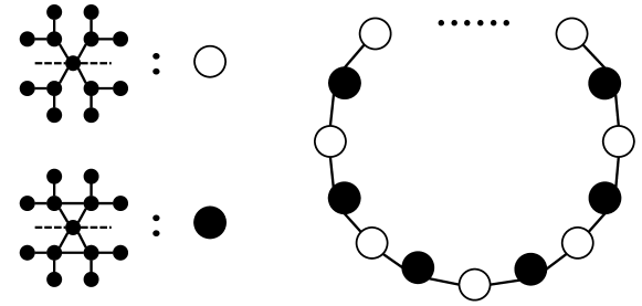
We first carry out visualization on an artificial dataset $\mathcal{G}(n)$ as a proof-of-concept, to test GNNs’ ability to identify local structural patterns. We build $\mathcal{G}(n)$ from a circle with $n$ nodes, where each node is surrounded by either two open or closed triads interleavingly. In addition, for each triad, there are 4 addition nodes linked to it. Apparently the nodes on the circle possess two distinct structural properties, those surrounded by closed triads and those by open ones. We show the illustration of $\mathcal{G}(n)$ and its building blocks in Fig. 4.

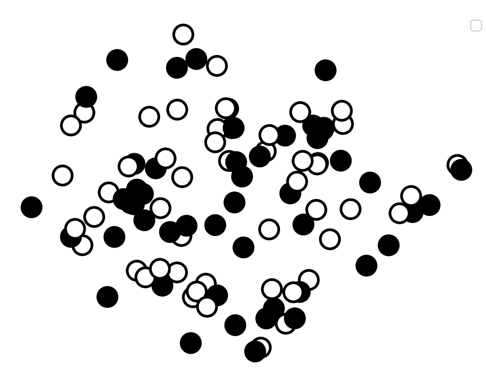
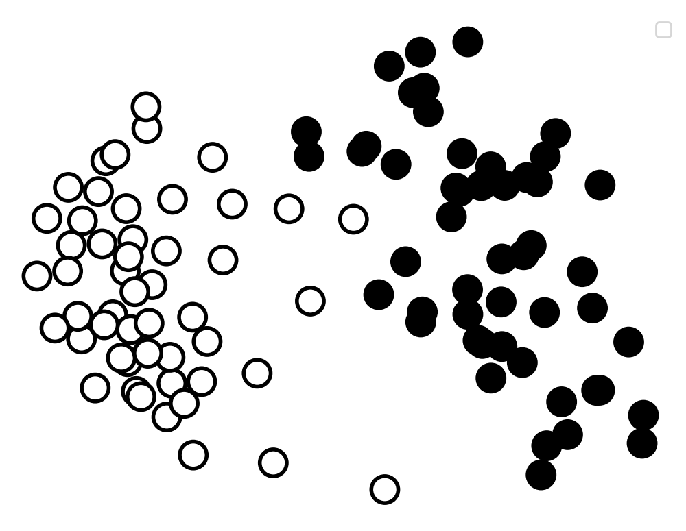
We visualize the representations from GraphSAGE and GraLSP in Fig. 4. As shown, GraLSP generates a clearer boundary between the two types of nodes, while GraphSAGE fails to draw a boundary as distinctive, which not only demonstrates the inability of current GNNs in generating distinctive embeddings for different local structural patterns, but also underscores the ability of anonymous walks and GraLSP in complementing such drawbacks.

(a) Illustration of $\mathcal{G}(n)$

(b) GraphSAGE

(c) GraLSP

Figure 4: Visualization on artificial graph $\mathcal{G}(100)$ where black dots denote nodes surrounded by closed triads and white ones denote those by open triads.

4.3 Node Classification

We carry out node classification on the four datasets. We learn representation vectors using the whole graph, which are then fed into Logistic Regression in Sklearn. We take 20% of all nodes as the test set and 80% as training. We take the macro and micro F1-scores for evaluation. In addition, all results are averaged for 10 independent experiments.

The results are shown in Table 2. As shown, the performance gain from original GNNs towards GraLSP is considerable, which demonstrates GraLSP is able to complement the drawbacks of identifying local structures. In addition, struc2vec and Graphwave perform poorly on academic datasets, but impressively on US-Airport, which can be attributed to the label definitions. In academic datasets, labels are defined as fields, where connected papers tend to have the same field and label, while in US-Airport, labels are taken as activity levels with less significant homophily but more related to structural properties. Nonetheless, we can see that generally GraLSP produces satisfactory results.

(a) Walks per node

(b) Anonym. walk length

(c) Walk loss weight

(d) Aggregation scheme

(e) Scalability

Figure 5: Results of Model Analysis

(a) DeepWalk

(b) struc2vec

(c) GraphSAGE

(d) GraLSP

Figure 6: Visualization of representation vectors from various algorithms in 2D space

4.4 Link Prediction

We then carry out link prediction under the same settings. We generate the test set by sampling 10% of the edges as positive edges, which are removed during training, with an identical number of random negative edges. For an edge $\langle i,j\rangle$, we take the inner product of their vectors $\mathbf{h}_{i}^{T}\mathbf{h}_{j}$, which will serve as the score for ranking. We take AUC and recall at 50% (equal to the number of positive edges) as metrics.

The results are shown in Table 3. It can be shown that our model is able to achieve gains compared to GCN, GraphSAGE and GAT, which should not be surprising given that structural patterns will shed light on possible edges (?), which are better captured by our model. Again, it is not surprising that struc2vec and Graphwave fail to generate satisfactory performances in that they assign similar representations to structurally similar nodes instead of connected nodes. As for US-Airport dataset, it is likely that local proximity is sufficient to reconstruct the graph, as shown by all baselines except LINE fail to perform well.

4.5 Model Analysis

We carry out tests on our model itself, including parameter analysis and scalability. Unless specified, we use node classification on Cora to reflect the performance of the model. All parameters are fixed as mentioned except those tested.

Number of Walks Sampled

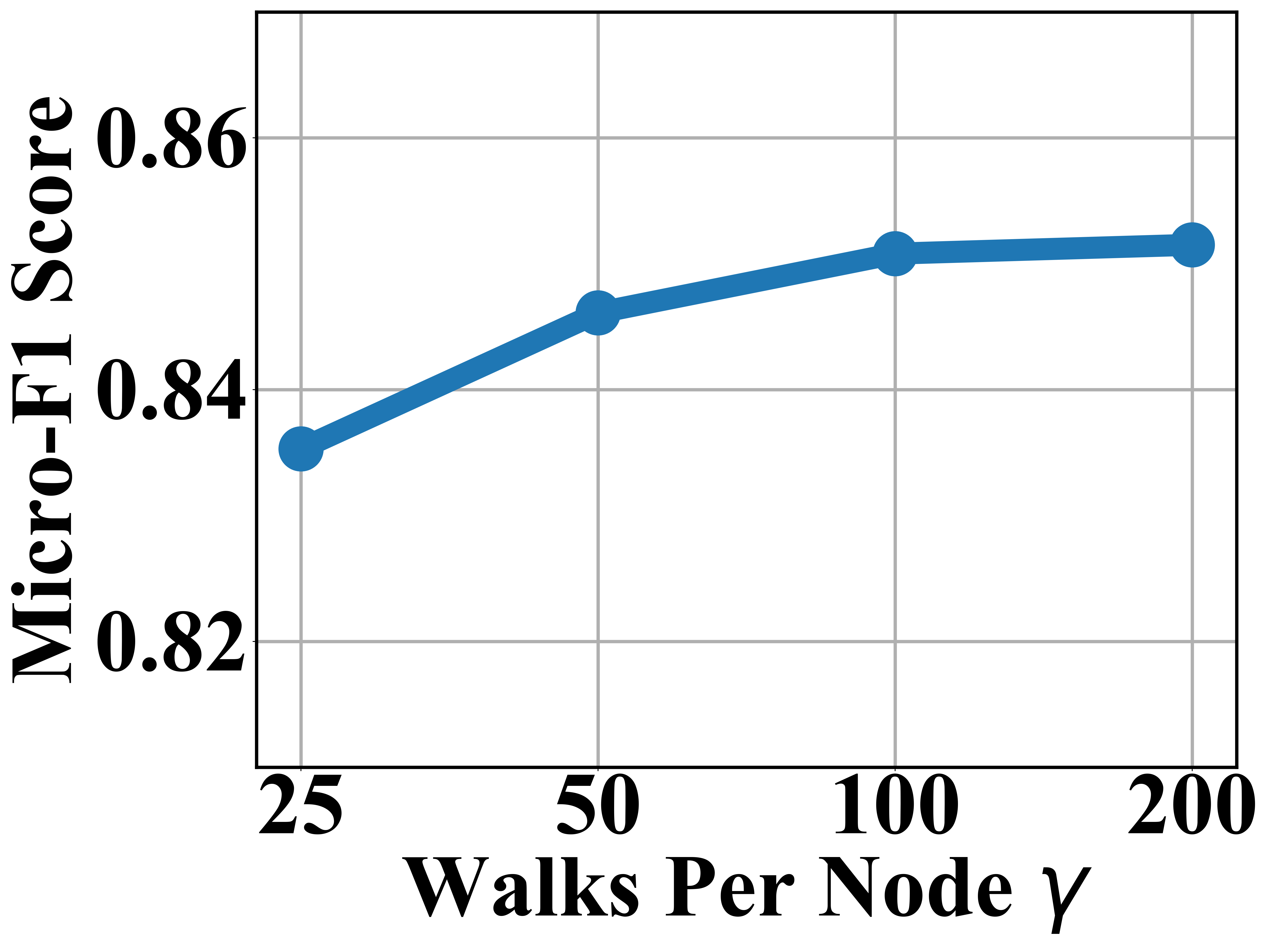
We run GraLSP with number of walks per node $\gamma=25,50,100,200$, and report their performances in Fig. 5(a). It can be shown that the more walks sampled each node, the better the performance. Empirically, as increasing $\gamma$ from 100 to 200 yields no significant gain, we conclude that $\gamma=100$ is reasonable in practice.

Length of Anonymous Walks

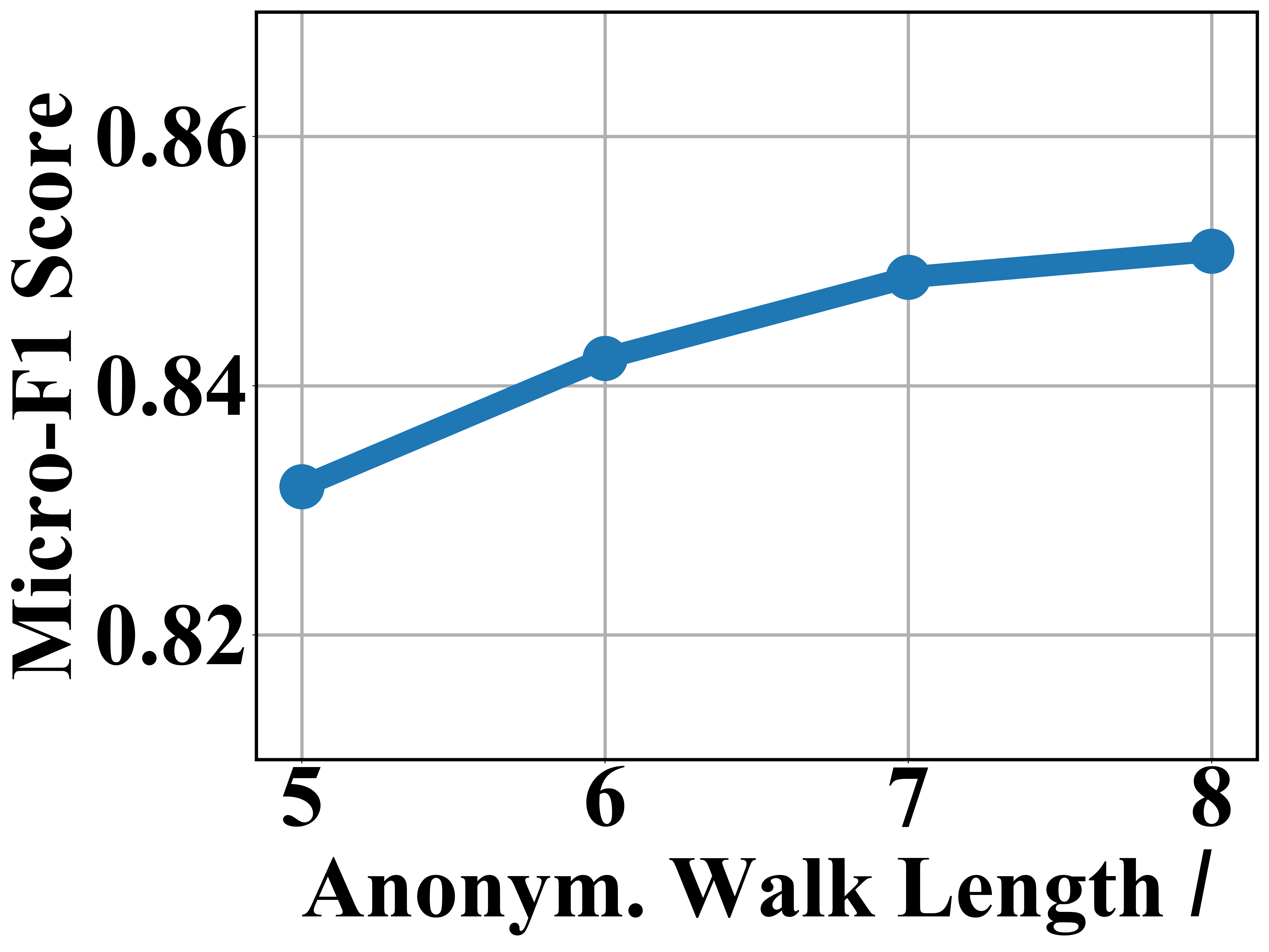
As longer walks are considered, more complex structural patterns are incorporated. We take $l=5,6,7,8$ and show the performances in Fig. 5(b). As shown, performance improves along with $l$, with decreasing marginal gains. As the number of anonymous walks grows exponentially with $l$, we conclude that $l=8$ would be sufficient in balancing efficiency and performance.

Weight of Objective Functions

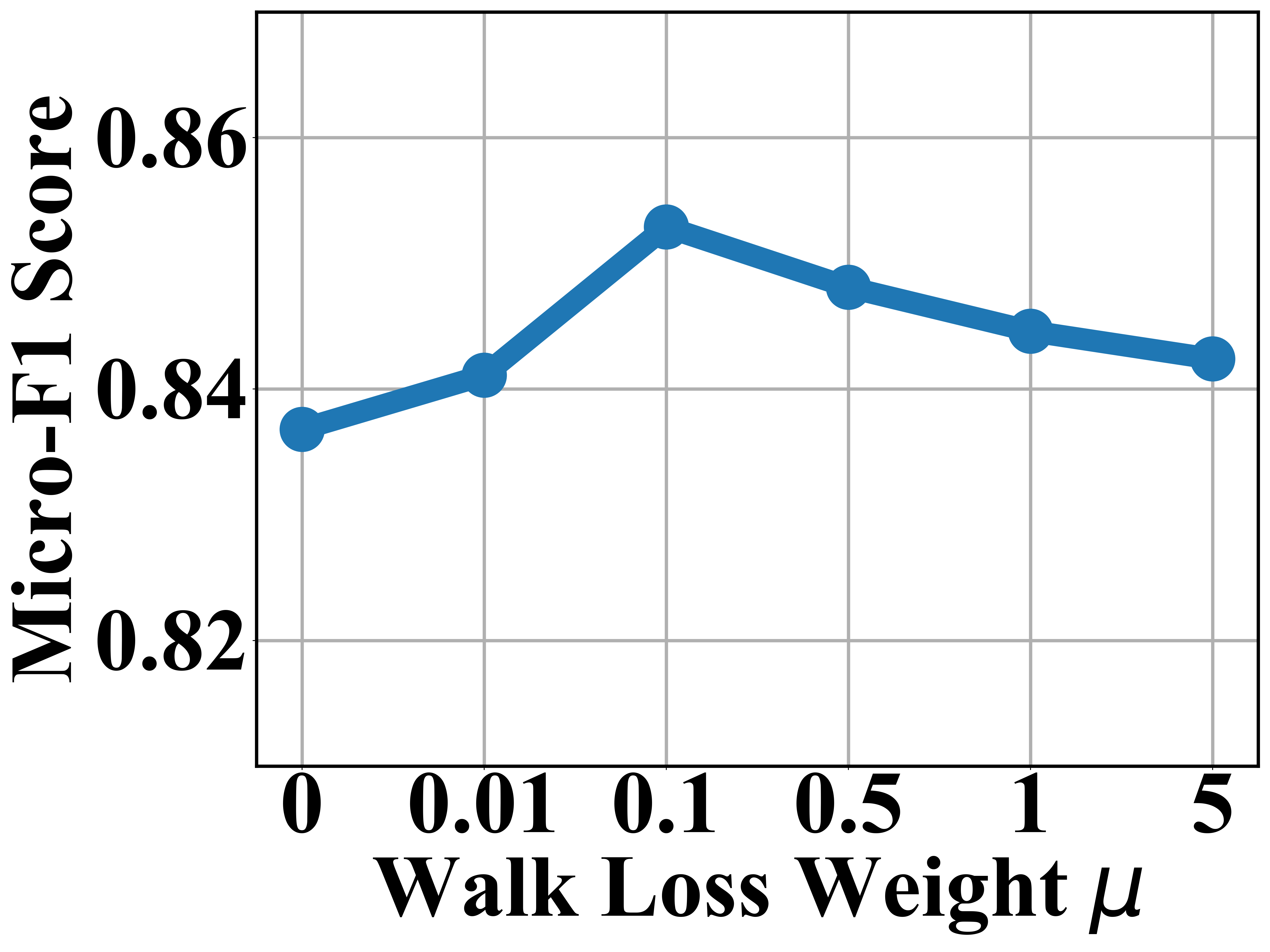
We analyze the weight of losses $\mu$, which determines the trade-off between the multi-task objective. We take $\mu=0,0.01,0.1,0.5,1,5$, and plot the performances in Fig. 5(c). It can be observed that starting from $\mu=0$, using only the objective in Eqn. 13, the performance peaks at $\mu=0.1$, before taking a plunge afterwards. We hence conclude that, the incorporation of our multi-task objective does enhance the performance of the model.

Study of Aggregation Scheme

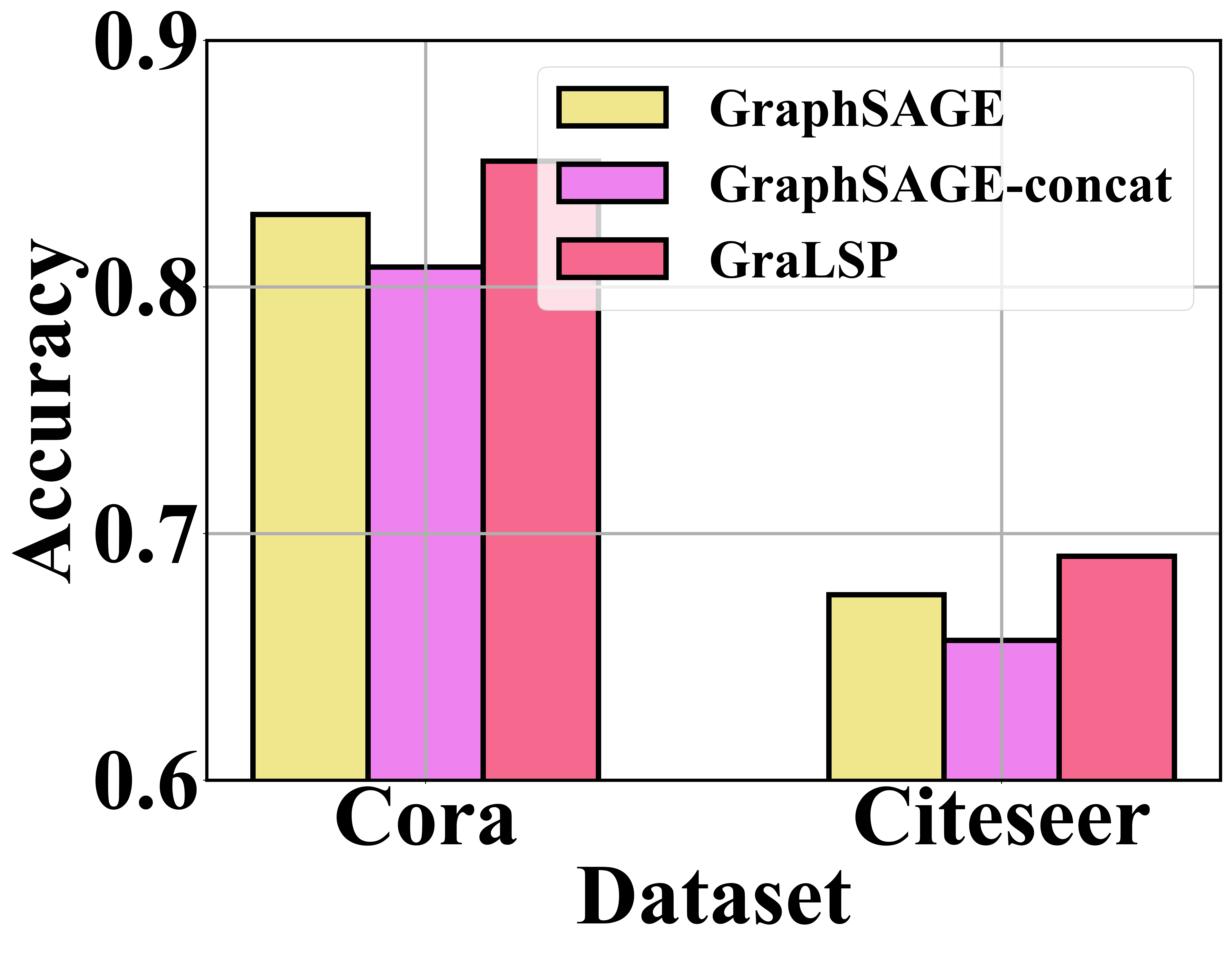
We analyze our aggregation scheme to verify that it enhances the aggregation of features. We compare our model with ordinary GraphSAGE, along with another GraphSAGE with node features concatenated with the distribution of anonymous walks, which proves to be a valid measure of structures (Ivanov (?)). We quote this variant as GraphSAGE-concat.

We show the results on Cora and Citeseer in Fig. 5(d). As shown, with node features concatenated with structural features, the GraphSAGE-concat did not even outperform GraphSAGE, which demonstrates that simply combining them would compromise both. By comparison, our model with adaptive receptive radius, attention and amplification outperforms both GraphSAGE and GraphSAGE-concat.

Scalability

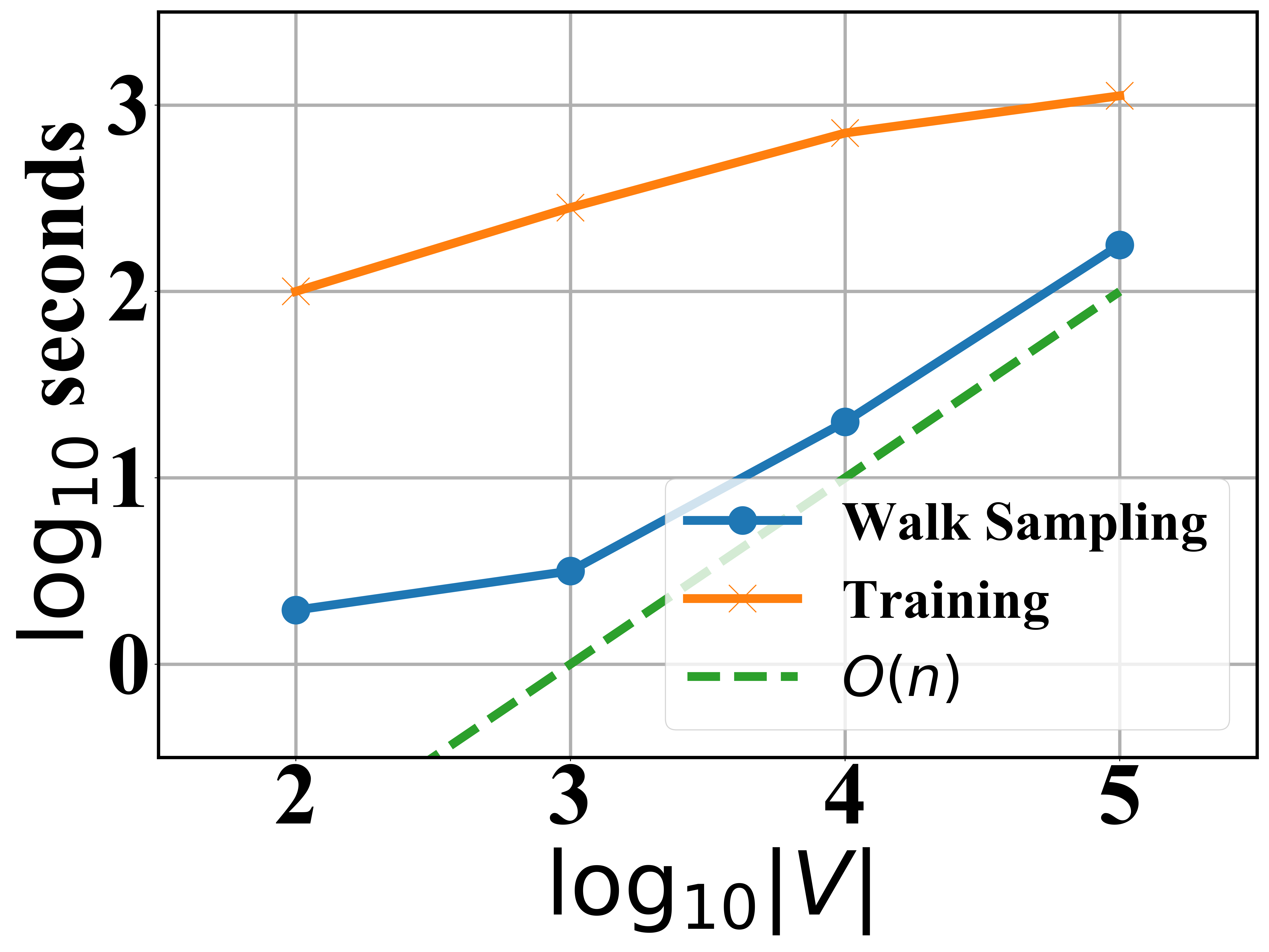
We finally analyze the scalability of our model. We run our model on Erdos-Renyi random graphs $G_{np}$ with $n=100,1000,10000,100000$ and $np=6$. We tested the time needed for the preprocessing (i.e. sampling random walks) and training to converge, which is defined by the loss not descending for 10 continuous iterations.

We plot the time needed with respect to the number of nodes in log-log scale in Fig. 5(e). As can be seen, both the preprocessing and the training time are bounded by an $O(n)$ complexity, which endorses the scalability of our model.

4.6 Visualization on Real World Datasets

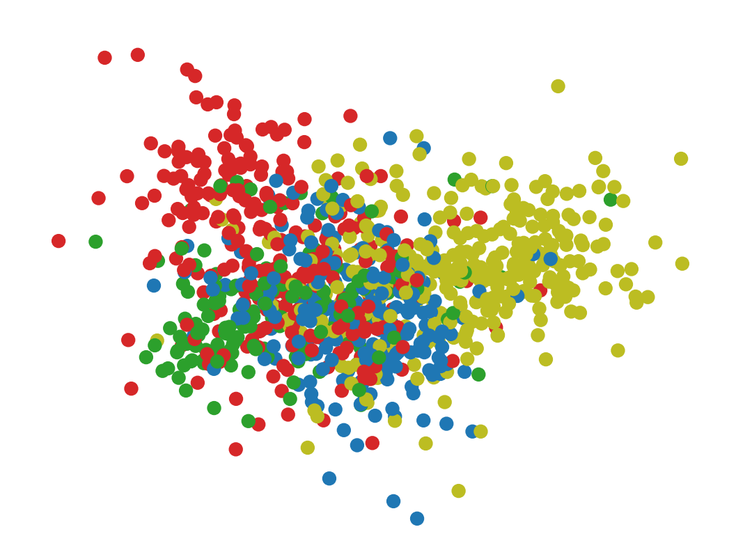
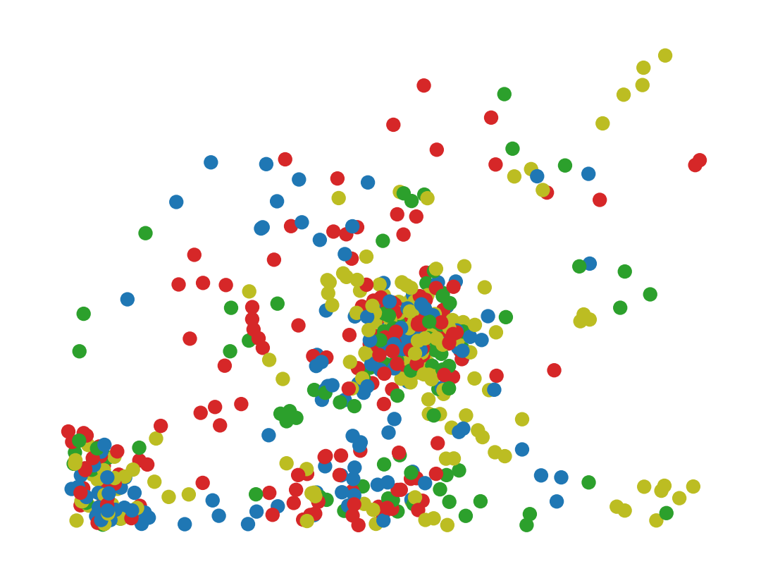
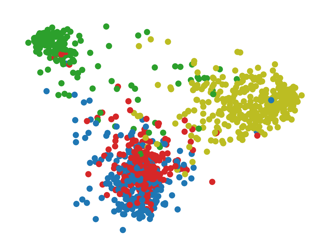
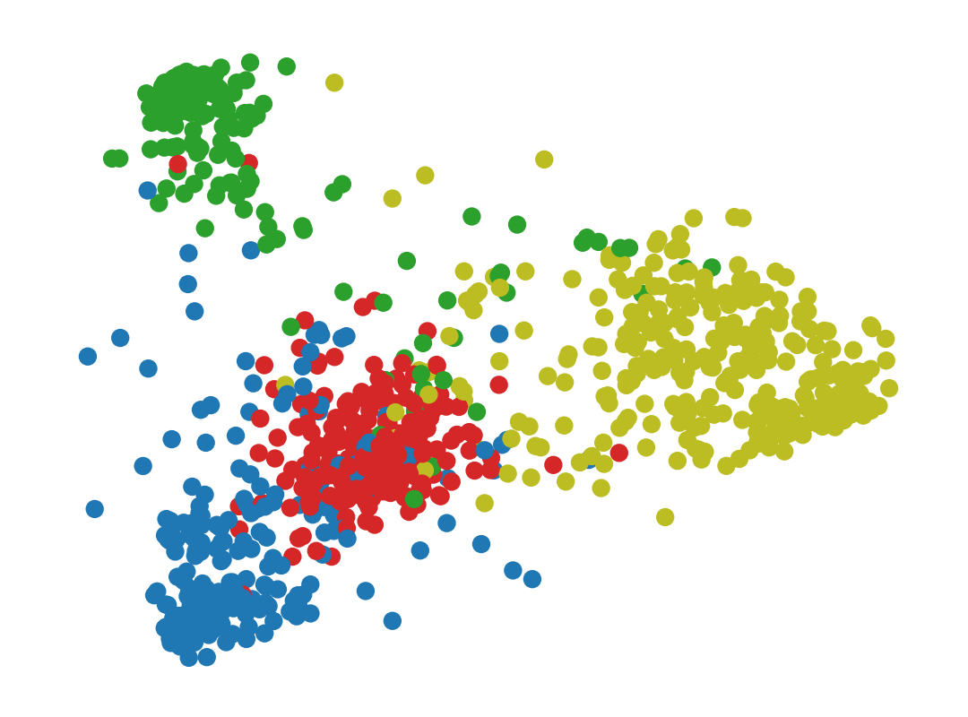
We finally carry out visualization on real world datasets to qualitatively evaluate our model. We learn the representation vectors on Cora, which are then reduced to 2-dimensional vectors using PCA. We select three representative models: DeepWalk (skip-gram), GraphSAGE (GNNs) and struc2vec (structure models), along with our model to compare.

The plots are shown in Fig. 6, where yellow, green, blue and red dots correspond to 4 labels within Cora. As shown, struc2vec (Fig. 6(b)) illustrates no clusters as connected nodes do not share similar representations. In addition, while DeepWalk (Fig. 6(a)), GraphSAGE (Fig. 6(c)) and GraLSP (Fig. 6(d)) all illustrate clustering among nodes with the same label, GraLSP generates clearer boundaries than DeepWalk and GraphSAGE (between blue and red dots).

5 Conclusion

We present a GNN framework incorporating local structural patterns to current GNNs, called GraLSP. We start by analyzing drawbacks of current GNNs in identifying local structural patterns, like triads. We then show that anonymous walks are effective alternatives in measuring local structural patterns, and represent them with vectors, which are incorporated into neighborhood aggregation with multiple modules. In addition, we present a multi-task objective preserving proximity between both pairwise nodes and walks. By adequately taking local structural patterns into account, our method outperforms several competitive baselines.

For future work, we plan to extend this paper to GNNs with more sophisticated architectures and more elaborate representations of local structures. In addition, interpretations of structures in GNNs will definitely improve our insight on various network phenomena.

References

- [2005] Borgwardt, K. M., and Kriegel, H.-P. 2005. Shortest-path kernels on graphs. In Fifth IEEE international conference on data mining (ICDM’05), 8–pp. IEEE.
- [2013] Bruna, J.; Zaremba, W.; Szlam, A.; and LeCun, Y. 2013. Spectral networks and locally connected networks on graphs. arXiv preprint arXiv:1312.6203.
- [2018] Chen, H.; Yin, H.; Wang, W.; Wang, H.; Nguyen, Q. V. H.; and Li, X. 2018. Pme: projected metric embedding on heterogeneous networks for link prediction. In Proceedings of the 24th ACM SIGKDD International Conference on Knowledge Discovery & Data Mining, 1177–1186. ACM.
- [2018] Cui, P.; Wang, X.; Pei, J.; and Zhu, W. 2018. A survey on network embedding. IEEE Transactions on Knowledge and Data Engineering.
- [2018] Donnat, C.; Zitnik, M.; Hallac, D.; and Leskovec, J. 2018. Learning structural node embeddings via diffusion wavelets. In Proceedings of the 24th ACM SIGKDD International Conference on Knowledge Discovery & Data Mining, 1320–1329. ACM.
- [1977] Granovetter, M. S. 1977. The strength of weak ties. In Social networks. Elsevier. 347–367.
- [2017] Hamilton, W.; Ying, Z.; and Leskovec, J. 2017. Inductive representation learning on large graphs. In Advances in Neural Information Processing Systems, 1024–1034.
- [2015] Huang, H.; Tang, J.; Liu, L.; Luo, J.; and Fu, X. 2015. Triadic closure pattern analysis and prediction in social networks. IEEE Transactions on Knowledge and Data Engineering 27(12):3374–3389.
- [2018] Ivanov, S., and Burnaev, E. 2018. Anonymous walk embeddings. In International Conference on Machine Learning, 2191–2200.
- [2016] Kipf, T. N., and Welling, M. 2016. Semi-supervised classification with graph convolutional networks. arXiv preprint arXiv:1609.02907.
- [2013] Kovanen, L.; Kaski, K.; Kertész, J.; and Saramäki, J. 2013. Temporal motifs reveal homophily, gender-specific patterns, and group talk in call sequences. Proceedings of the National Academy of Sciences 110(45):18070–18075.
- [2018] Li, Q.; Han, Z.; and Wu, X.-M. 2018. Deeper insights into graph convolutional networks for semi-supervised learning. In Thirty-Second AAAI Conference on Artificial Intelligence.
- [2019] Liu, Z.; Chen, C.; Li, L.; Zhou, J.; Li, X.; Song, L.; and Qi, Y. 2019. Geniepath: Graph neural networks with adaptive receptive paths. In Proceedings of the AAAI Conference on Artificial Intelligence, volume 33, 4424–4431.
- [2019] Long, Q.; Wang, Y.; Du, L.; Song, G.; Jin, Y.; and Lin, W. 2019. Hierarchical community structure preserving network embedding: A subspace approach. In Proceedings of the 28th ACM International Conference on Information and Knowledge Management, 409–418. ACM.
- [2016] Micali, S., and Zhu, Z. A. 2016. Reconstructing markov processes from independent and anonymous experiments. Discrete Applied Mathematics 200:108–122.
- [2019] Morris, C.; Ritzert, M.; Fey, M.; Hamilton, W. L.; Lenssen, J. E.; Rattan, G.; and Grohe, M. 2019. Weisfeiler and leman go neural: Higher-order graph neural networks. In Proceedings of the AAAI Conference on Artificial Intelligence, volume 33, 4602–4609.
- [2016] Niepert, M.; Ahmed, M.; and Kutzkov, K. 2016. Learning convolutional neural networks for graphs. In International conference on machine learning, 2014–2023.
- [2000] Ogata, H.; Fujibuchi, W.; Goto, S.; and Kanehisa, M. 2000. A heuristic graph comparison algorithm and its application to detect functionally related enzyme clusters. Nucleic acids research 28(20):4021–4028.
- [2017] Paranjape, A.; Benson, A. R.; and Leskovec, J. 2017. Motifs in temporal networks. In Proceedings of the Tenth ACM International Conference on Web Search and Data Mining, 601–610. ACM.
- [2014] Perozzi, B.; Al-Rfou, R.; and Skiena, S. 2014. Deepwalk: Online learning of social representations. In Proceedings of the 20th ACM SIGKDD international conference on Knowledge discovery and data mining, 701–710. ACM.
- [2007] Pržulj, N. 2007. Biological network comparison using graphlet degree distribution. Bioinformatics 23(2):e177–e183.
- [2017] Ribeiro, L. F.; Saverese, P. H.; and Figueiredo, D. R. 2017. struc2vec: Learning node representations from structural identity. In Proceedings of the 23rd ACM SIGKDD International Conference on Knowledge Discovery and Data Mining, 385–394. ACM.
- [2008] Scarselli, F.; Gori, M.; Tsoi, A. C.; Hagenbuchner, M.; and Monfardini, G. 2008. The graph neural network model. IEEE Transactions on Neural Networks 20(1):61–80.
- [2009] Shervashidze, N.; Vishwanathan, S.; Petri, T.; Mehlhorn, K.; and Borgwardt, K. 2009. Efficient graphlet kernels for large graph comparison. In Artificial Intelligence and Statistics, 488–495.
- [2015] Tang, J.; Qu, M.; Wang, M.; Zhang, M.; Yan, J.; and Mei, Q. 2015. Line: Large-scale information network embedding. In Proceedings of the 24th international conference on world wide web, 1067–1077. International World Wide Web Conferences Steering Committee.
- [2017] Veličković, P.; Cucurull, G.; Casanova, A.; Romero, A.; Lio, P.; and Bengio, Y. 2017. Graph attention networks. arXiv preprint arXiv:1710.10903.
- [2017] Wang, X.; Cui, P.; Wang, J.; Pei, J.; Zhu, W.; and Yang, S. 2017. Community preserving network embedding. In Thirty-First AAAI Conference on Artificial Intelligence.
- [2018] Xu, K.; Hu, W.; Leskovec, J.; and Jegelka, S. 2018. How powerful are graph neural networks? arXiv preprint arXiv:1810.00826.
- [2018] Ying, R.; He, R.; Chen, K.; Eksombatchai, P.; Hamilton, W. L.; and Leskovec, J. 2018. Graph convolutional neural networks for web-scale recommender systems. In Proceedings of the 24th ACM SIGKDD International Conference on Knowledge Discovery & Data Mining, 974–983. ACM.
- [2019] Zhang, Y.; Song, G.; Du, L.; Yang, S.; and Jin, Y. 2019. Dane: Domain adaptive network embedding. In Proceedings of the Twenty-Eighth International Joint Conference on Artificial Intelligence, IJCAI-19, 4362–4368. International Joint Conferences on Artificial Intelligence Organization.
- [2018] Zhou, J.; Cui, G.; Zhang, Z.; Yang, C.; Liu, Z.; and Sun, M. 2018. Graph neural networks: A review of methods and applications. arXiv preprint arXiv:1812.08434.