Full distribution of first exit times in the narrow escape problem

Abstract

In the scenario of the narrow escape problem (NEP) a particle diffuses in a finite container and eventually leaves it through a small "escape window" in the otherwise impermeable boundary, once it arrives to this window and over-passes an entropic barrier at the entrance to it. This generic problem is mathematically identical to that of a diffusion-mediated reaction with a partially-reactive site on the container’s boundary. Considerable knowledge is available on the dependence of the mean first-reaction time (FRT) on the pertinent parameters. We here go a distinct step further and derive the full FRT distribution for the NEP. We demonstrate that typical FRTs may be orders of magnitude shorter than the mean one, thus resulting in a strong defocusing of characteristic temporal scales. We unveil the geometry-control of the typical times, emphasising the role of the initial distance to the target as a decisive parameter. A crucial finding is the further FRT defocusing due to the barrier, necessitating repeated escape or reaction attempts interspersed with bulk excursions. These results add new perspectives and offer a broad comprehension of various features of the by-now classical NEP that are relevant for numerous biological and technological systems.

1 Introduction

The Narrow Escape Problem (NEP) describes the search by a diffusing particle for a small "escape window" (EW) in the otherwise impermeable boundary of a finite domain (figure 1) [1, 2]. The NEP represents a prototypical scenario, inter alia, in biophysics, biochemistry, molecular and cell biology, and in nanotechnology. Specifically, the particle could be an ion, a chemically active molecule or a protein confined in a biological cell, a cellular compartment or a microvesicle. The EW could be a veritable "hole" in the boundary, for instance, a membrane pore, but it could also represent a reactive site right inside (or on) the boundary, such as a protein receptor waiting to be triggered by a specific diffusing molecule. Similarly, the NEP may pertain to a tracer molecule trying to leave from an interstice in the porous structure of an underground aquifer. When one is solely interested in how the particle reaches the target, the NEP corresponds to the first-passage time problem [3]. The situation becomes more complicated when some further action is needed after the EW is reached. For instance, the particle may have to react chemically with an imperfect, partially-reactive site, which will require the crossing of an activation energy barrier. To produce a successful reaction event the particle may repeatedly need to revisit the target after additional rounds of bulk diffusion. Similarly, when the particle has to leave the domain through a pore or a channel, an entropy barrier due to the geometric confinement at the entrance to the EW needs to be over-passed [4]. In these scenarios, the relevant quantities are the first-reaction or first-exit times, which are often substantially longer than the first-passage time to the EW. For brevity, in what follows we will call the first-passage times to the successful reaction event as the first-reaction time (FRT), for both the eventual passage through the EW constrained by an entropic barrier or for the reaction with a partially reactive site. This is a random variable dependent on a variety of physical parameters and here we unveil its non-trivial statistical properties.

The paradigmatic NEP has been extensively studied in terms of mean FRTs [2, 5, 6, 7]. While early analyses concentrated on idealised, spherically-symmetric domains enclosed by a perfect hard-wall with a perfect (that is, barrierless) EW [8, 9, 10, 11, 12, 13, 14], more recent work examined the NEP for domains with more complicated geometries and non-smooth boundaries, when, e.g., a perfect barrierless target is hidden in a cusp or screened by surface irregularities [15, 16, 17, 18, 19]. A striking example of the NEP with very severe escape restrictions is the dire strait problem [20]. Effects of short-ranged (contact) and long-ranged interactions with the confining boundary, which are quite ubiquitous and give rise to "intermittent motion" characterised by alternating phases of bulk and surface diffusion, were shown to allow for an optimisation of the search times [21, 22, 23, 24, 4, 25, 26]. It was also studied how molecular crowding in cellular environments impacts the search dynamics [13, 27, 28]. When the target is imperfect the contributions due to diffusive search and penetration through a barrier were shown to enter additively to the mean FRT [29, 4, 30, 31], akin to the celebrated Collins-Kimball relation in chemical kinetics [32]. Since these two rate-controlling factors disentangle the concept of search- versus barrier-controlled NEP was proposed [4, 30].

Despite of this considerable body of works published on the NEP, information beyond the mean FRT is scarce, only two recent analytical and numerical works consider the full distributions of first-passage times to perfect targets and only in two-dimensional settings [33, 34]. In fact, the NEP typically involves a broad spectrum of time scales giving rise to a rich and interesting structure of the probability density function (PDF) of FRTs with different time regimes. Knowledge of this full PDF is therefore a pressing case. As we show here the FRT may be strongly defocused over several orders of magnitude, effecting noticeable trajectory-to-trajectory fluctuations [35]. One therefore cannot expect that, in general, solely the first moment of the PDF can be sufficient to characterise its form exhaustively well. Moreover, it is quite common that the behaviour of the positive moments of a distribution is dominated by its long-time tail and, hence, stems from anomalously long and rarely observed trajectories [36, 35, 37]. Fluctuations between realisations are indeed common in diffusive processes and can be characterised by the amplitude fluctuations of time-averaged moments [38, 39] and single-trajectory power spectra [40, 41, 42].

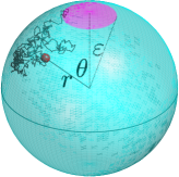
Figure 1: Spherical domain of radius $R$ containing a target (a partially reactive site or an EW) depicted as a spherical cap (in magenta) of a polar angle $\varepsilon$ located at the North pole. The red dot denotes the starting point $(r,\theta)$ of the diffusing particle, and the zigzag line depicts a random diffusive path to the target.

We here present the PDF of the FRTs for the NEP in the generic case of a spherical domain with an imperfect target and an arbitrary fixed starting point of the diffusing particle. Indeed, in cellular environments, this setting represents one of the most interesting applications of the NEP, as particles such as small signalling molecules or proteins are usually released at some fixed point inside the cell [43] and need to diffusively locate specific targets such as channel or receptor proteins embedded in the cell membrane [44, 45]. Our analytical approach is based on a self-consistent closure scheme [46, 4, 47] that yields analytical results in excellent agreement with numerical solutions. We demonstrate that in these settings the PDF exhibits typically four distinct temporal regimes delimited by three relevant time scales, for which we also present explicit expressions. These characteristic times may differ from each other by several orders of magnitude. We fully characterise the PDF of FRTs by identifying the cumulative reaction depths (the fractions of FRT events corresponding to each temporal regime of the PDF) and analyse their dependence on the system parameters. Overall, our analysis provides a first complete and comprehensive framework for the understanding of multiple facets of the biologically and technologically relevant NEP, paving a way for a better theoretical understanding of the NEP and a meaningful interpretation of experimental data. Last but not least, it permits for a straightforward derivation of the first-reaction time PDF for a more general problem with several diffusive particles starting their random motion from given locations. In appendices, we also discuss the forms of the PDF and the relevant time scales for other possible initial conditions.

2 The Narrow Escape Problem

As depicted in figure 1 we consider a diffusing point-like particle with diffusion coefficient $D$ inside a spherical domain of radius $R$. The boundary enclosing the domain is perfectly reflecting everywhere, except for the imperfect target – a spherical cap of angle $\varepsilon$ at the North pole. By symmetry, the behaviour is independent of the azimuthal angle, and we need to solve the diffusion equation for the survival probability $S(r,\theta;t)$ that a particle released at position ${\bf r}=(r,\theta)$ at time $0$ has not reacted with the partially-reactive site or has not escaped through the EW up to time $t$. The diffusion equation is completed by the initial condition $S(r,\theta;t=0)=1$ and by the mixed boundary conditions of zero-current at the hard wall combined with the standard Collins-Kimball partially-reactive (or partially-reflecting) boundary condition imposed at the EW or the chemically-active site [32] (see also [48, 49] for an overview)

$$-\left.D\frac{\partial S(r,\theta;t)}{\partial r}\right|_{r=R}=\left\{\begin{array}[]{ll}\kappa\,S(R,\theta;t)&(0\leq\theta<\varepsilon),\\ 0&(\varepsilon\leq\theta\leq\pi).\\ \end{array}\right.$$ (1)

The latter Robin boundary condition signifies that the reaction is a two-stage process consisting of a) the diffusive transport of the particle to the vicinity of the target and b) the eventual imperfect reaction which happens with a finite probability. The proportionality factor $\kappa$ here is the intrinsic reactivity, which is defined as $\kappa=\omega l$, where $l$ is the effective "thickness" of the reaction zone in the vicinity of the target – the minimal reaction distance, while $\omega$ is the rate (frequency) describing the number of elementary reaction acts per unit of time within the volume of the reaction zone. Clearly, $\omega$ (and hence, $\kappa$) depends on the amplitude of the barrier against the reaction event: $\omega=\infty$ ($\kappa=\infty$) corresponds to the case of a perfect barrierless reaction or an immediate escape upon the first encounter with the EW. In this case the FRT reduces to the first-passage time to the target. Conversely, $\omega=0$ ($\kappa=0$) implies that the reaction/escape event is completely suppressed. In our calculations, we suppose that $\kappa$ is a given parameter (for heterogeneous, space-dependent reactivity, see [50] and references therein). In Section 4, we will elaborate on possible distinctions between its values for reaction and escape processes. Once $S(r,\theta;t)$ is obtained, the PDF $H(r,\theta;t)$ of the FRT is given by the negative derivative of the survival probability with respect to $t$. Further details on the NEP, our analytical derivation, and the comparison with numerical results are presented in appendices.

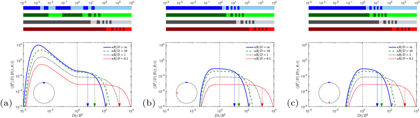
Figure 2: PDF $H(r,\theta;t)$ of FRTs, from Eq. (2), rescaled by $R^{2}/D$, as function of $Dt/R^{2}$ for $r/R=0.9$, $\varepsilon=0.1$, four values of the dimensionless reactivity $\bar{\kappa}=\kappa R/D$ indicated in the panels, and (a) $\theta=0$, (b) $\theta=\pi/2$, (c) $\theta=\pi$. Insets in all panels indicate schematically the location of the starting point shown by red circle, with respect to the target (blue) placed at the North pole. Note that $\bar{\kappa}$ includes $R$ and $D$ such that at fixed $\kappa$, smaller values of $\bar{\kappa}$ can be achieved by lowering $R$ or increasing $D$. The approximation in (2) is truncated to $n=50$ terms. Vertical arrows indicate the mean FRT $t_{\rm mean}$. The dashed vertical line shows the crossover time $t_{c}=R^{2}/D$, at which the particle first engages with the boundaries. The coloured bar-codes above each main panel indicate the cumulative reaction depths corresponding to the four values of $\bar{\kappa}$, in decreasing order from top to bottom. Each bar-code is split into ten regions of alternating brightness, representing the ten $10\%$-quantiles of the PDF. The numbers on top of the bar-codes indicate the values of $Dt/R^{2}$. For example, in panel (a) the first dark blue region for the case $\bar{\kappa}=\infty$ (perfect reaction or no entropic barrier at the EW) indicates that $10\%$ of reaction events occur up to $Dt/R^{2}\approx 3\times 10^{-3}$, which is close to the dimensionless most probable FRT $Dt_{\rm mp}/R^{2}$. The mean FRT $t_{\rm mean}$ in this case is almost four orders of magnitude longer than the most probable FRT $t_{\rm mp}$, and over $70\%$ of trajectories arrive to the target up to this time. Analogous estimates of the cumulative reaction depths for other initial conditions are presented in the text below and also in appendices.

3 Results

Our principal analytical result is the explicit, approximate expression for the PDF $H(r,\theta;t)$ of the FRT,

$$H(r,\theta;t)=\frac{D}{R^{2}}\sum\limits_{m=0}^{\infty}e^{-Dt\alpha_{m}^{2}/R^{2}}v_{m}(r,\theta),$$ (2)

with

$$v_{m}(r,\theta)=\frac{2}{F^{\prime}(\alpha_{m})}\sum\limits_{n=0}^{\infty}\phi_{n}(\varepsilon)P_{n}(\cos\theta)\frac{j_{n}(\alpha_{m}r/R)}{-j^{\prime}_{n}(\alpha_{m})},$$ (3)

$$\phi_{n}(\varepsilon)=\frac{P_{n-1}(\cos\varepsilon)-P_{n+1}(\cos\varepsilon)}{1-\cos\varepsilon}\quad(n=1,2,\ldots),$$ (4)

where $\phi_{0}(\varepsilon)=1$, $P_{n}\left(\cos\varepsilon\right)$ are the Legendre polynomials, $j_{n}(z)$ are the spherical Bessel functions of the first kind, the prime denotes the derivative with respect to the argument, while $\alpha_{m}$ are the positive solutions (organised in ascending order) of the transcendental equation

$$\sum_{n=0}^{\infty}\frac{\phi_{n}^{2}\left(\varepsilon\right)}{\left(2n+1\right)}\frac{j_{n}(\alpha)}{\alpha j^{\prime}_{n}(\alpha)}\equiv F(\alpha)=-\frac{2D}{\kappa R\left(1-\cos\varepsilon\right)}.$$ (5)

Equations (2) to (5) completely determine the explicit form of $H(r,\theta;t)$. As we already mentioned above, this result is obtained by resorting to a self-consistent closure scheme, developed earlier for the calculation of the mean FRT in certain reaction-diffusion problems [46, 4, 47]. This approximation consists in replacing the actual mixed boundary condition (1) by an inhomogeneous Neumann condition and in the derivation of an appropriate closure relation, which ensures that the mixed boundary condition (1) holds on average. The adaptation of such a scheme to the calculation of the full PDF in NEP is discussed in detail in A and B. We note that despite an approximate character of our approach, the obtained result turns out to be very accurate for arbitrary starting position $(r,\theta)$ (although not too close to the target), for a very wide range of $\varepsilon$, and for arbitrary value of $\kappa$. The accuracy was checked by comparing our approximation to a numerical solution of the original problem by a finite-elements method (see E). We note, as well, that two important characteristic length-scales can be read off directly from expression (2) and are associated with the smallest and the second smallest solutions of (5), (that being, $\alpha_{0}$ and $\alpha_{1}$), which define the largest and the second largest decay times of the PDF, respectively. The analysis of all the solutions of (5), which define the full form of the PDF valid at arbitrary times, their relation to the characteristic time scales, the derivations of the asymptotic forms of $H(r,\theta;t)$, and its easy-to-implement approximate mathematical form are provided in the appendices. The latter also present a variety of other useful results based on $H(r,\theta;t)$, e.g., the surface-averaged and volume-averaged PDFs (see Eqs. (51) and (52)).

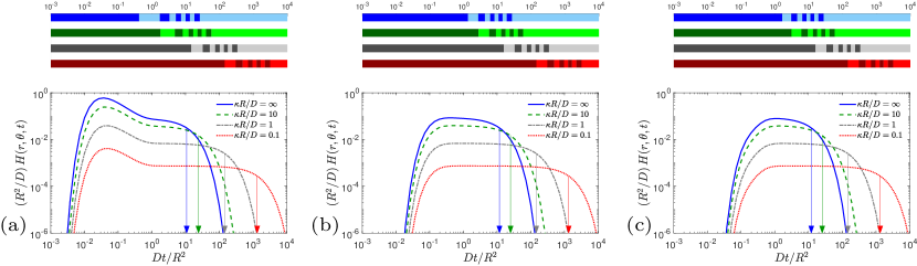
Figure 3: PDF $H(r,\theta;t)$ of the FRT, determined from (2) to (5) and rescaled by $R^{2}/D$, as function $Dt/R^{2}$ for $r/R=0.5$, $\varepsilon=0.1$, several values of dimensionless reactivity $\bar{\kappa}=\kappa R/D$ (indicated in the plots), and $\theta=0$ (a), $\theta=\pi/2$ (b), $\theta=\pi$ (c). Self-consistent approximation is truncated to $n=50$ terms. Vertical arrows indicate the mean FRT, $t_{\rm mean}$. Coloured bar-codes above each figure indicate the cumulative depths corresponding to four considered values of $\bar{\kappa}$, in decreasing order from top to bottom. Each bar-code is split into ten regions of alternating brightness, each representing ten $10\%$-quantiles of the distribution. The numbers on top of the bar-codes indicate the values of $Dt/R^{2}$. For example, in panel (a) the first dark blue region for the case $\bar{\kappa}=\infty$ (perfect reaction) indicates that $10\%$ of reaction events occur till $Dt/R^{2}\simeq 3\times 10^{-1}$. The dimensionless mean FRT in this case is around $10^{1}$, i.e., is almost two orders of magnitude bigger that $Dt_{\rm mp}/R^{2}$, and over $70\%$ of all trajectories arrive to the target up to this time.

In figure 2 we depict the PDF $H(r,\theta;t)$ defined by (2) to (5) for three different fixed initial positions (polar angles $\theta=0$ (a), $\theta=\pi/2$ (b), and $\theta=\pi$ (c), with fixed $r/R=0.9$), four values of the intrinsic reactivity $\kappa$, and for a particular choice $\varepsilon=0.1$. We observe that the PDF has a clearly defined structure, which depends on whether the starting point is close to the target or not. In the former case (as in panel (a)), the PDF consists of a hump-like region around the most probable FRT $t_{\rm mp}$, an extended plateau-like region after the crossover time $t_{\rm c}$ (remarkably, within this region all values of the FRT are nearly equally probable), and, ultimately, exponential decay starting right after the mean FRT $t_{\rm mean}$. Note that up to $t_{\rm mean}$ the particle experiences multiple collisions with the boundary of the container after unsuccessful reactions, thereby loosing the memory about its precise starting location. Due to this circumstance, the ultimate, long-time exponential decay (which is the most trivial part of the PDF), holds for all bounded domains, regardless of the precise initial condition (see also appendices). As evidenced in figure 2 the difference between $t_{\rm mp}$, $t_{\rm c}$ and $t_{\rm mean}$ may span orders of magnitude revealing a pronounced defocusing of the FRTs (see below). In contrast, when the starting point is far from the target (panels (b) and (c)), the hump-like region is much less apparent, and the extended plateau and the exponential decay are the major features of the PDF. Although the maximum of the PDF formally exists, the corresponding most probable time is not informative because the escape (or reaction) may happen at any moment over the plateau region with almost equal probabilities. We note that the overall shape of the curves presented in figure 2 is generic and gets only slightly modified upon parameter changes – see, e.g., figure 3 in appendices in which a similar plot for $r/R=0.5$ is presented. Note, as well, that the behaviour of the PDF in the case when the starting point is uniformly distributed over a spherical surface some distance $r$ away from the origin, appears to be very similar to the one depicted in figure 2 in panels (b) and (c) (see figure 4, panel (b)). Conversely, in the case when the location of the starting point is random and uniformly distributed over the volume of the container, the PDF consists essentially of a plateau-like region and the ultimate exponential tail (see figure 4 (a)).

The existence of the hump-like region is not an unexpected feature in the case of a fixed initial condition. For a particle initially placed some distance away from the target, it is impossible to reach the latter instantaneously such that the probability of having a very short FRT is close to zero. This defines the most probable reaction time $t_{\rm mp}$, which can be estimated as function of the initial distance $\sigma$ to the target (in panel (a) of Fig. 2, $\sigma=R-r$ as $\theta=0$) in the form (see appendices),

$$t_{\rm mp}\lesssim(R-r)^{2}/(2D).$$ (6)

The most probable FTR corresponds to "direct" trajectories [51] on which the particle moves fairly straight to the target, with immediate successful reaction. Consequently the value of $t_{\rm mp}$ is "geometry-controlled" [51, 52] by the initial distance $R-r$. At such short time scales, the particle has not yet explored the boundaries of the domain, and thus the initial increase up to $t_{\rm mp}$ and the subsequent power-law descent of the PDF are well-described by the Lévy-Smirnov-type law $A\exp(-\alpha/t)/t^{3/2}$ [3] (see C.2 for more details). In our case of an imperfect target, the amplitude $A$ also acquires the dependence on the reactivity $\kappa$ and the target radius $\rho$. In particular, the descent from the peak value of the PDF obeys

$$H(r,\theta;t)\simeq\frac{\rho}{\sqrt{4\pi Dt^{3}}}\frac{\frac{D}{\kappa\rho}+\frac{\sigma}{\sigma+\rho}}{(1+\frac{D}{\kappa\rho})^{2}}\,.$$ (7)

The independence on the domain size stems from the fact that the particle at such short times has no knowledge about the boundaries.

The hump-like region is delimited by the crossover time

$$t_{\rm c}\approx R^{2}/D,$$ (8)

an important characteristic time-scale, at which the particle first engages with the domain boundaries and realises that it lives in a bounded domain. The plateau-like regime, which sets in at $t_{\rm c}$, is a remarkable feature for the NEP that has not been reported in literature on this important and generic problem. The existence of such a plateau for diffusion-reaction systems with an activation energy barrier at the target has only been recently discovered in other geometrical settings, such as, e.g., the diffusive search for a partially-reactive site placed on a hard-wall cylinder confined in a cylindrical container [47] and a spherical target at the centre of a larger spherical domain [52]. The fact that it also appears in typical NEP settings, as shown here, evidences that it is a fundamental feature of systems in which the reaction event requires not only a diffusive search but also a barrier crossing.

The plateau typically persists for several decades in time, up to the mean FRT $t_{\rm mean}$ (indicated by vertical arrows in figure 2), which is very close (but not exactly equal) to the decay-time $t_{\rm d}=1/(D\lambda_{0})$, associated with the smallest eigenvalue $\lambda_{0}$ of the Laplace operator (see appendices for more details). As a consequence, the FRT PDF features the exponential shoulder

$$H(r,\theta;t)\sim\exp\left(-t/t_{\rm d}\right).$$ (9)

Note that the right-tail of the PDF is thus fully characterised by the unique time scale $t_{\rm d}$. For a perfectly-reactive target, the asymptotic behaviour of $t_{\rm d}$ in the narrow-escape limit (i.e., for $\varepsilon\to 0$) was first obtained by Lord Rayleigh [8] more than a century ago within the context of the theory of sound, and then refined and adapted for the NEP by Singer et al. [10], yielding (see also discussions in appendices and in [53, 54, 55])

$$t_{\rm d}\simeq\frac{3R^{2}}{\pi D}\varepsilon^{-1}\qquad(\varepsilon\to 0).$$ (10)

For an imperfect target, however, this asymptotic result is no longer valid and one finds instead that (see appendices)

$$t_{\rm d}\simeq\frac{2R}{3\kappa(1-\cos\varepsilon)}\simeq\frac{4R}{3\kappa}\varepsilon^{-2}\qquad(\varepsilon\to 0)$$ (11)

which signifies that the decay time diverges much faster when $\varepsilon\to 0$, as compared to the case of a perfect barrierless target. Lastly, we note that the fact that $t_{\rm mean}$ and $t_{\rm d}$ appear very close to each other is an apparent consequence of the existence of the plateau region with an exponential cut-off, suggesting that the major contribution to $t_{\rm mean}$ (and most likely to all positive moments of the PDF) is dominated by the integration over this temporal regime.

4 Discussion

The results presented above reveal many interesting and novel features of the NEP that we now put into more general context.

i) In case of chemical reactions with a partially-reactive site, the intrinsic reactivity $\kappa$ is independent of $\varepsilon$. As a consequence, $t_{\rm d}$ in Eq. (11) (as well as $t_{\rm mean}$, see appendices) diverges in the NEP limit as $t_{\rm d}\sim 1/\varepsilon^{2}$. The situation is much more delicate in the case of an entropy barrier $\Delta S$. The impeding effect of the latter has been studied in various guises, including transport in narrow channels with corrugated walls (see, e.g., [56, 57, 58, 59, 60]) and also for the NEP (see, e.g., [61, 62]), although for the latter problem no explicit results have been presented. In particular, for diffusion in channels represented as a periodic sequence of broad chambers and bottlenecks, the influential works [56, 58] expressed this barrier through a profile $h(x)$ of the channel cross-section, while in [60], for ratchet-like channels, this barrier was estimated as $\Delta S\sim\beta^{-1}\ln\left(h_{\rm max}/h_{\rm min}\right)$, where $\beta$ is the reciprocal temperature, $h_{\rm max}$ and $h_{\rm min}$ are the maximal and minimal channel apertures (a chamber versus a bottleneck). Therefore, one may expect that for the NEP the entropic barrier scales as $\Delta S\sim\beta^{-1}\alpha\ln\left(1/\varepsilon\right)$, where $\alpha>0$ is a numerical constant characterising the precise form of the profile $h(x)$. Assuming that the particle penetrates through the barrier solely due to a thermal activation, i.e., that $\kappa\sim\exp(-\beta\Delta S)$, one expects then that $\kappa\sim\varepsilon^{\alpha}$ and thus vanishes in the NEP limit $\varepsilon\to 0$. This means, in turn, that here $t_{\rm d}\sim 1/\varepsilon^{2+\alpha}$, i.e., $t_{\rm d}$ diverges more strongly in the NEP limit than its counterpart in the case of a partially-reactive site. As a consequence, the overall effect of such an entropy barrier on the size of the plateau region and on the cumulative reaction depth on this temporal stage, is much more significant for the NEP than for diffusion-reaction systems. Importantly, both for the NEP and for reactions with a partially-reactive site, as $\varepsilon\to 0$, the mean FRT is always controlled by the penetration through the barrier rather than by the stage of random search for the target whose contribution to $t_{\rm d}$ diverges in the leading order only as $1/\varepsilon$.

We also remark that, of course, the NEP limit has to be understood with an appropriate caution: taking $\varepsilon\to 0$, one descends to molecular scales at which both the molecular structure of the container’s boundaries, surface irregularities, presence of contaminants and other chemically active species come into play. At such scales, the solvent can also be structured close to the wall, affecting characteristic diffusion times and hence, the value of the diffusion coefficient $D$. Moreover, the size of a particle does matter here and one can no longer consider it as point-like. The entropic barrier is then a function of the ratio between the particle radius $a$ and the radius $\rho$ of the EW. Understanding theoretically the functional form of $\kappa$ is so far beyond reach and one may address the problem only by numerical simulations or experiments. We are, however, unaware of any systematic approach to these issues, except for a recent paper [63], which studied the particle-size effect on the entropic barriers via numerical simulations. It was observed that the dependence of the inverse transition rate (and hence, of $\kappa$) of a Brownian particle in a model system consisting of a necklace of hard-wall spheres connected to each other by EWs, can be well-fitted by an empirical law of the form $\kappa\sim\left(1-a/\rho\right)^{3/2}$ signifying that $\kappa$ vanishes very rapidly when $a\to\rho$. When the particle size $a$ is comparable to that of the EW, the entropic barrier becomes very high resulting in a significant decrease of $\kappa$. Some other effects of the particle size and shape onto diffusive search, unrelated to our work, were discussed in [64, 65].

ii) The concept of the search-controlled versus barrier-controlled NEP proposed in [4, 30] holds indeed for the mean FRT, see Eq. (71). In contrast, we observe that two other important characteristic time-scales – $t_{\rm mp}$ and $t_{\rm c}$ – are unaffected by the reactivity and solely depend on the diffusion coefficient and the geometry. This means that the two controlling factors represented by $\kappa$ and $D$ do not disentangle. Moreover, both affect the shape of the PDF and the corresponding cumulative reaction depths.

iii) For the NEP with fixed starting point of the particle the characteristic time-scales $t_{\rm mp}$, $t_{\rm c}$ and $t_{\rm mean}$ differ by orders of magnitude meaning that the FRT are typically very defocused. This is a conceptually important point for the understanding of the NEP, but alone it does not provide a complete picture. Indeed, one should also analyse the cumulative reaction depths corresponding to each temporal regime. For example, for the settings used in figure 2 (panel (a)), the shortest relevant time-scale is $t_{\rm mp}$. For perfect, barrierless reactions the amount of reaction events appearing up to this quite short time $(Dt/R^{2}\approx 10^{-3})$ is surprisingly non negligible, being of the order of $10$ per cent. Upon lowering the dimensionless reactivity $\bar{\kappa}=\kappa R/D$ (i.e., upon increase of the activation barrier at the target or of the diffusion coefficient $D$, or upon lowering $R$), this amount drops significantly and the contribution of "direct" trajectories becomes less important. This is quite expected because the latter now very rarely lead to the reaction event. In turn, the contribution of the whole hump-like region (for $t$ stretching up to $t_{\rm c}$) for barrierless reactions is more than $50$ per cent, meaning that more than a half of all reaction events take place up to the time-scale when the particle first realises that it moves in a confined domain. One infers next from figure 2 (panel (a)) that upon lowering $\bar{\kappa}$, this amount also drops rapidly. At the same time, the plateau-like region becomes increasingly more pronounced for smaller $\bar{\kappa}$ and progressively more reaction events take place during this stage: we find $25$, $30$, $47$ and $55$ per cent of all reaction events for $\bar{\kappa}=\infty$, $10$, $1$ and $0.1$, respectively. Interestingly, the fraction of "unsuccessful trajectories", which survive up to the largest characteristic time $t_{\rm mean}$, appears to be very weakly dependent on the value of $\bar{\kappa}$, and is rather universally about $30$ per cent. Note that this number is close to the fraction of outcomes of an exponentially distributed random variable above its mean, $\exp(-1)\simeq 0.37$. Therefore, even for this particular case when the starting point is very close to the target, one observes a rather diverse behaviour – there is no apparent unique time-scale and no overall dominant temporal regime: the region with the rise to the most probable value, the one with the subsequent descent to the plateau, the plateau-like region itself, and the eventual exponential decay may all become relevant for different values of the parameters and hence, their respective contributions depend on the case at hand. This illustrates our earlier statement that the knowledge of the full PDF of FRT is indispensable for the proper understanding of distinct facets of the NEP.

For a random starting point, when it is either uniformly distributed over the volume, or is located at a random point on a distance $r$ away from the origin, the situation is somewhat different. Here, the hump-like region is smeared away and the PDF consists of just two regions: a plateau-like region and the ultimate exponential decay. As a consequence, in these cases $t_{\rm mean}$ is a unique characteristic time-scale, as it was claimed previously (see, e.g. [7]). In appendices, we present explicit results for the general case of diffusion-mediated reactions with an activation energy barrier and imperfect EW with an entropy barrier. Concerning the cumulative reaction depths in case of a random starting point, we observe an analogous surprising behaviour to what was noted above: the cumulative reaction depth over the plateau region (up to $t_{\rm mean}$) appears to be rather universally (i.e., independent of $\kappa$ and other parameters) equal to $\approx 70$ per cent, while the remaining $\approx 30$ per cent of trajectories react within the final exponential stage.

iv) Apart from the analysis of the cumulative depths, it is helpful to work out an explicit approximate formula for the PDF, which may be used to fit experimental or numerical data. In appendices, we outline a derivation of such a formula, which agrees very well for the whole range of variation of the FRT.

v) One often deals with situations when several diffusing particles, starting at some fixed points, are present in a biophysical system and the desired random event is triggered by the one, which arrives first to a specific site on the surface of the container. Among many examples (see e.g. [66]), one may mention, for instance, calcium ions which activate calcium release in the endoplasmic reticulum at neuronal synapses. Our results for the fixed starting-point PDF $H(r,\theta;t)$ and the corresponding survival probability provide the desired solution to this problem too. As a matter of fact, if the particles are present at a nanomolar concentration, such that their dynamics are independent, the probability that neither of the particles arrived to the target site up to time $t$ is just the product of the single-particle survival probabilities. The PDF of the time of the first reaction event then follows by a mere differentiation of this product.

5 Conclusion

With modern optical microscopy, production events of single proteins [43], their passage through the cell [67] as well as single-molecule binding events [68, 69] can be monitored in living biological cells [70]. Typical processes in cells such as gene expression involve the production of proteins at a specific location, their diffusive search for their designated binding site, and the ultimate reaction with this partially-reactive site [71, 72]. Given the often minute, nanomolar concentrations of specific signalling molecules in cells, the first-reaction time PDF of a diffusing molecule with its target in the cell volume was shown to be strongly defocused and geometry-controlled [51, 47, 52]. These analyses demonstrate that the concept of mean FRTs (or reaction rates) is no longer adequate in such settings involving very low concentrations. Here one invariably needs knowledge of the full PDF to describe such systems faithfully.

Complementary to this situation when a particle is released inside a finite volume and needs to react with a target somewhere else in this volume, we here analysed the important case when a diffusing particle is released inside a bounded volume and needs to react with a target on the boundary. Our results for the FRT PDF including the passage of an energetic or entropic barrier leading to final reaction with the target or the crossing of the escape window, demonstrate a pronounced defocusing of time scales. While the most likely FRT corresponds to a direct particle trajectory to the target and immediate reaction, indirect paths decorrelating the initial position by interaction with the boundary are further emphasised by unsuccessful reaction events, leading to further rounds of exploration of the bulk. This effect is shown to imply a pronounced defocusing, and thus a large reaction depth is reached long before the mean FRT. In particular, we demonstrate that the shapes of the PDF are distinctly different from the case when the particle needs to react with a target inside the volume of the bounded domain.

Our findings have immediate relevance to biological cells, in which specific molecules released in the cell need to locate and bind to receptors on the inside of the cell wall, or they need to pass the cell wall or compartment membrane through protein channels or membrane pores. Similar effects occur in inanimate systems, when chemicals in porous aquifers need to leave interstices through narrow holes in order to penetrate further. From a technological perspective our results will find applications in setups involving lipid bilayer micro-reaction containers linked by tubes [73].

References

Appendix A Solution in Laplace domain

Our starting point is the diffusion equation for the survival probability $S(r,\theta;t)$ of a particle started at position $(r,\theta)$ inside a sphere of radius $R$, up to time $t$:

$$\partial_{t}S(r,\theta;t)=D\Delta S_{t}(r,\theta),$$ (12)

subject to the initial condition $S(r,\theta;t=0)=1$ and the mixed boundary conditions:

$$-D\bigl{(}\partial_{n}S(r,\theta;t)\bigr{)}_{r=R}=\left\{\begin{array}[]{l l}\kappa S(R,\theta;t)&(0\leq\theta<\varepsilon),\\ 0&(\varepsilon\leq\theta\leq\pi),\\ \end{array}\right.$$ (13)

where $\partial_{n}=\partial_{r}$ is the normal derivative directed outwards the ball, $\Delta$ the Laplace operator, $D$ the diffusion coefficient, $\kappa$ the intrinsic reactivity, and $\varepsilon$ the angular size of the escape window (or target site) at the North pole (Fig. 1).

The Laplace transform of the survival probability,

$$\tilde{S}(r,\theta;p)=\int\limits_{0}^{\infty}dt\,e^{-pt}\,S(r,\theta;t),$$ (14)

satisfies the modified Helmholtz equation

$$(p-D\Delta)\tilde{S}(r,\theta;p)=1,$$ (15)

subject to the same mixed boundary condition:

$$-D\bigl{(}\partial_{r}\tilde{S}(r,\theta;p)\bigr{)}_{r=R}=\left\{\begin{array}[]{l l}\kappa\tilde{S}(R,\theta;p)&(0\leq\theta<\varepsilon),\\ 0&(\varepsilon\leq\theta\leq\pi).\\ \end{array}\right.$$ (16)

According to the self-consistent approximation [46, 4, 47], we substitute this mixed boundary condition by an effective inhomogeneous Neumann condition:

$$-D\bigl{(}\partial_{r}\tilde{S}(r,\theta;p)\bigr{)}_{r=R}=Q\,\Theta(\varepsilon-\theta),$$ (17)

where $Q$ is an effective flux to be computed, and $\Theta$ is the Heaviside step function.

We search the solution of the modified problem in (15), (17) in the form

$$\tilde{S}(r,\theta;p)=u_{0}(r)+\frac{R^{2}}{D}\sum\limits_{n=0}^{\infty}a_{n}g_{n}(r)P_{n}(\cos\theta),$$ (18)

where $u_{0}(r)$ is the solution of (15) with the Dirichlet boundary condition, $u_{0}(r)=\frac{1}{p}(1-g_{0}(r)/g_{0}(R))$, $P_{n}(z)$ are the Legendre polynomials, $a_{n}$ are the unknown coefficients to be determined, and $g_{n}(r)$ are the radial functions satisfying

$$g^{\prime\prime}_{n}+\frac{2}{r}g^{\prime}_{n}-\frac{n(n+1)}{r^{2}}g_{n}-\frac{p}{D}g_{n}=0,$$ (19)

where prime denotes the derivative with respect to $r$. A solution of this equation, which is regular at $r=0$, is the modified spherical Bessel function of the first kind, which reads as

$$g_{n}(r){\color[rgb]{0,0,0}=i_{n}\bigl{(}r\sqrt{p/D}\bigr{)}}=\frac{\sqrt{\pi}}{\sqrt{2}}\,\frac{I_{n+1/2}\bigl{(}r\sqrt{p/D}\bigr{)}}{\bigl{(}r\sqrt{p/D}\bigr{)}^{1/2}}\,,$$ (20)

where $I_{\nu}(z)$ is the modified Bessel function of the first kind, and we fixed a particular normalisation (as shown below, the result does not depend on the normalisation).

Substituting (18) into the modified boundary condition in (17), multiplying by $P_{n}(\cos\theta)\sin\theta$ and integrating over $\theta$ from $0$ to $\pi$, one gets

$$2D\biggl{(}\frac{g^{\prime}_{0}(R)}{pg_{0}(R)}-\frac{R^{2}}{D}a_{0}g^{\prime}_{0}(R)\biggr{)}=Q(1-\cos\varepsilon)\quad(\textrm{for}~{}n=0),$$ (21)

and

$$-2R^{2}a_{n}g^{\prime}_{n}(R)=Q\bigl{(}P_{n-1}(\cos\varepsilon)-P_{n+1}(\cos\varepsilon)\bigr{)}\quad(\textrm{for}~{}n>0).$$ (22)

Combining these results, we can express $a_{n}$ as

$$a_{n}=-\frac{\phi_{n}(\varepsilon)g^{\prime}_{0}(R)}{g^{\prime}_{n}(R)}\biggl{(}\frac{D}{pR^{2}}\frac{1}{g_{0}(R)}-a_{0}\biggr{)}\qquad(n=1,2,\ldots),$$ (23)

where

$$\phi_{n}(\varepsilon)=\frac{P_{n-1}(\cos\varepsilon)-P_{n+1}(\cos\varepsilon)}{1-\cos\varepsilon}\qquad(n=1,2,\ldots).$$ (24)

The remaining coefficient $a_{0}$ is determined by requiring that the mixed boundary condition in (16) is satisfied on average on the target, i.e.,

$$-D\int\limits_{0}^{\varepsilon}d\theta\,\sin\theta\,\bigl{(}\partial_{r}\tilde{S}(r,\theta;p)\bigr{)}_{r=R}=\int\limits_{0}^{\varepsilon}d\theta\,\sin\theta\,\kappa\tilde{S}(R,\theta;p).$$ (25)

Using (17) and (21) for the left-hand side of this relation and substituting (18) into the right-hand side, one gets

$$2D\biggl{(}\frac{g^{\prime}_{0}(R)}{pg_{0}(R)}-\frac{R^{2}}{D}a_{0}g^{\prime}_{0}(R)\biggr{)}=\kappa\frac{R^{2}}{D}\sum\limits_{n=0}^{\infty}a_{n}g_{n}(R)\frac{(1-\cos\varepsilon)\phi_{n}(\varepsilon)}{2n+1}\,,$$ (26)

where we completed (24) by setting $\phi_{0}(\varepsilon)\equiv 1$. Expressing $a_{n}$ via (23), one obtains a closed expression for $a_{0}$

$$a_{0}=\frac{D}{pR^{2}g_{0}(R)}\biggl{(}1-\frac{g_{0}(R)}{Rg^{\prime}_{0}(R)}\eta_{p}\biggr{)},$$ (27)

where

$$\eta_{p}=\biggl{(}\frac{2D}{\kappa R(1-\cos\varepsilon)}+\mathscr{R}_{\varepsilon}\biggr{)}^{-1}\,,$$ (28)

with

$$\mathscr{R}_{\varepsilon}=\sum\limits_{n=0}^{\infty}\frac{g_{n}(R)}{Rg^{\prime}_{n}(R)}\,\frac{\phi_{n}^{2}(\varepsilon)}{2n+1}\,.$$ (29)

From (23), we get thus

$$a_{n}=-\frac{\phi_{n}(\varepsilon)}{Rg^{\prime}_{n}(R)}\frac{D}{pR^{2}}\eta_{p},$$ (30)

and finally

$$\tilde{S}(r,\theta;p)=\frac{1}{p}\biggl{(}1-\eta_{p}\sum\limits_{n=0}^{\infty}\phi_{n}(\varepsilon)\frac{g_{n}(r)}{Rg^{\prime}_{n}(R)}P_{n}(\cos\theta)\biggr{)}.$$ (31)

As a consequence, the Laplace-transformed probability density function of the FPT, $\tilde{H}(r,\theta;p)=1-p\tilde{S}(r,\theta;p)$, reads

$$\tilde{H}(r,\theta;p)=\eta_{p}\sum\limits_{n=0}^{\infty}\phi_{n}(\varepsilon)\frac{g_{n}(r)}{Rg^{\prime}_{n}(R)}P_{n}(\cos\theta).$$ (32)

As mentioned above, the solution does not depend on the normalisation of functions $g_{n}(r)$, as they always enter as a ratio of $g^{\prime}_{n}$ and $g_{n}$. One can check that the probability density function $H(r,\theta;t)$ is correctly normalised, i.e., $\tilde{H}(r,\theta;p=0)=1$. In fact, one has in the limit $p\to 0$:

$$\frac{g_{0}(r)}{Rg^{\prime}_{0}(R)}\to\infty,\qquad\frac{g_{n}(r)}{Rg^{\prime}_{n}(R)}\to\frac{(r/R)^{n}}{n}\quad(n=1,2,\ldots)$$ (33)

so that the term with $n=0$ dominates both in $\eta_{p}$ and in the series in (32).

When the starting point is uniformly distributed over a spherical surface of radius $r$, the surface average yields

$$\overline{\tilde{H}(p)}_{r}\equiv\frac{1}{4\pi}\int\limits_{0}^{\pi}d\theta\,\sin\theta\int\limits_{0}^{2\pi}d\phi\,\tilde{H}(r,\theta;p)=\eta_{p}\frac{g_{0}(r)}{Rg^{\prime}_{0}(R)}\,.$$ (34)

In turn, if the starting point is uniformly distributed in the volume of the ball, one gets the volume average

$$\overline{\tilde{H}(p)} \equiv \frac{1}{4\pi R^{3}/3}\int\limits_{0}^{R}dr\,r^{2}\int\limits_{0}^{\pi}d\theta\,\sin\theta\int\limits_{0}^{2\pi}d\phi\,\tilde{H}(r,\theta;p)$$ (35)

$$= \frac{3\eta_{p}}{R\sqrt{p/D}}\frac{g_{1}(R)}{Rg_{0}^{\prime}(R)}=\frac{3\eta_{p}}{R^{2}p/D}\,.$$

The explicit expressions (32), (34), and (35) for the Laplace-transformed PDF present one of the main results. We recall that (32) is the exact solution of the modified Helmholtz equation in (15), in which the mixed boundary condition (16) is replaced by an effective inhomogeneous Neumann condition (17). As a consequence, (32) and its volume and surface averages in (34) and (35) are approximate solutions to the original problem. In E, we compare these approximate solutions to the numerical solution of the original problem obtained by a finite-elements method (FEM). We show that the approximate solutions are remarkably accurate for a broad range of $p$, for both narrow ($\varepsilon=0.1$) and extended ($\varepsilon=1$) targets.

It is worth mentioning that the developed self-consistent approximation can also be applied to the exterior problem when a particle is released outside a ball of radius $R$ and searches for a target on its boundary. The derivation follows the same lines, with two minor changes: (i) the modified Bessel function of the first kind in Eq. (20) should be replaced by the modified Bessel function of the second kind, i.e.

$$g_{n}(r)=\frac{\sqrt{2}}{\sqrt{\pi}}\,\frac{K_{n+1/2}(r\sqrt{p/D})}{(r\sqrt{p/D})^{1/2}}\,,$$ (36)

and (ii) the normal derivative is directed inside the sphere so that the sign of all radial derivatives should be modified. As a consequence, the former expressions (32), (34), (35) remain valid, except that Eq. (28) is replaced by

$$\eta_{p}=\biggl{(}\mathscr{R}_{\varepsilon}-\frac{2D}{\kappa R(1-\cos\varepsilon)}\biggr{)}^{-1}\,.$$ (37)

Appendix B Solution in time domain

To get the probability density function $H(r,\theta;t)$ in time domain, we need to perform the inverse Laplace transform of $\tilde{H}(r,\theta;p)$ from (32). As diffusion occurs in a bounded domain, the spectrum of the underlying Laplace operator is discrete and is determined by the poles of $\tilde{H}(r,\theta;p)$, considered as a function of a complex-valued parameter $p$. We note first that the zeros of the functions $g_{0}(R)$ and $g^{\prime}_{n}(R)$, standing in the denominator of $\tilde{H}(r,\theta;p)$, are not the poles, as the corresponding divergence is compensated by vanishing of the function $\eta_{p}$ at these points. So, we are left with the poles of the function $\eta_{p}$ from (28) which are determined by the following equation on $p\in{\mathbb{C}}$:

$$\sum\limits_{n=0}^{\infty}\frac{\phi_{n}^{2}(\varepsilon)}{2n+1}\,\frac{g_{n}(R)}{Rg^{\prime}_{n}(R)}=-\frac{2D}{\kappa R(1-\cos\varepsilon)}\,.$$ (38)

As the eigenvalues are positive, the poles lie on the negative real axis of the complex plane: $p<0$. Setting $R\sqrt{p/D}=i\alpha$, one has

$$g_{n}(R)=i^{n}j_{n}(\alpha),\qquad Rg^{\prime}_{n}(R)=i^{n}\,\alpha j^{\prime}_{n}(\alpha),$$ (39)

where

$$j_{n}(z)=\sqrt{\pi/2}\,\frac{J_{n+1/2}(z)}{\sqrt{z}}$$ (40)

are the spherical Bessel functions of the first kind.

Substituting these relations into (38), one gets the following transcendental equation:

$$F(\alpha)=-\frac{2D}{\kappa R(1-\cos\varepsilon)}\,,$$ (41)

where

$$F(\alpha)\equiv\sum\limits_{n=0}^{\infty}\frac{\phi_{n}^{2}(\varepsilon)}{2n+1}\,\frac{j_{n}(\alpha)}{\alpha\,j^{\prime}_{n}(\alpha)}\,.$$ (42)

Let us denote by $\alpha_{m}$ all positive solutions of (41). The numerical computation of these zeros employs the monotonous increase of $F(\alpha)$ that can be checked by evaluating its derivative,

$$F^{\prime}(\alpha)=\sum\limits_{n=0}^{\infty}\frac{\phi_{n}^{2}(\varepsilon)}{2n+1}\,\frac{\alpha^{2}[j^{\prime}_{n}(\alpha)]^{2}+\alpha j_{n}(\alpha)j^{\prime}_{n}(\alpha)+[\alpha^{2}-n(n+1)][j_{n}(\alpha)]^{2}}{\alpha^{3}[j^{\prime}_{n}(\alpha)]^{2}},$$ (43)

and recognising that the numerator of the second factor is proportional a positive integral:

$$\frac{2}{\alpha}\int\limits_{0}^{\alpha}dx\,x^{2}\,j_{n}^{2}(x)=\alpha^{2}[j^{\prime}_{n}(\alpha)]^{2}+\alpha j_{n}(\alpha)j^{\prime}_{n}(\alpha)+[\alpha^{2}-n(n+1)][j_{n}(\alpha)]^{2}\,,$$ (44)

which is actually the standard normalisation of spherical Bessel functions. For each $n=0,1,2,\ldots$, let $\alpha_{nk}^{0}$ ($k=0,1,2,\ldots$) denote all positive zeros of the function $j^{\prime}_{n}(z)$. Putting all these zeros in an increasing order, we call the elements of this sequence by $\alpha_{m}^{0}$ (i.e., $\alpha_{m}^{0}=\alpha_{nk}^{0}$ for some indices $n$ and $k$). At each $\alpha_{m}^{0}$, the function $F(\alpha)$ diverges. As a consequence, one can search for zeros $\alpha_{m}$ on intervals between two successive zeros $\alpha_{m}^{0}$ and $\alpha_{m+1}^{0}$. As the function $F(\alpha)$ is continuous on each such interval and monotonously increasing, there is precisely one solution of (41) on each interval. The solution can be easily found by bisection or Newton’s method. This observation implies that all poles are simple. Moreover, the second eigenvalue $\lambda_{1}=\alpha_{1}^{2}/R^{2}$ is bound from below as

$$\lambda_{1}\geq(\alpha_{10}^{0})^{2}/R^{2}>4/R^{2},$$ (45)

where $\alpha_{1}^{0}=\alpha_{10}^{0}=2.081575978\ldots$ is the smallest strictly positive zero of $j^{\prime}_{1}(z)$ (i.e., the right-hand side is the first strictly positive eigenvalue of the Laplace operator for the full reflecting sphere). As expected, this bound is independent of the target size and determines the crossover time $t_{c}$ that we set as

$$t_{c}=\frac{R^{2}}{D}$$ (46)

(as a qualitative border between two regimes, $t_{c}$ is determined up to an arbitrary numerical factor that we select here to be $1$).

The Laplace transform can now be inverted by the residue theorem that yields

$$H(r,\theta;t)=\frac{D}{R^{2}}\sum\limits_{m=0}^{\infty}e^{-Dt\alpha_{m}^{2}/R^{2}}\,v_{m}(r,\theta),$$ (47)

where

$$v_{m}(r,\theta)\equiv\frac{2}{F^{\prime}(\alpha_{m})}\sum\limits_{n=0}^{\infty}\phi_{n}(\varepsilon)P_{n}(\cos\theta)\frac{j_{n}(\alpha_{m}r/R)}{-j^{\prime}_{n}(\alpha_{m})}\,.$$ (48)

Note that the sign minus in front of $j^{\prime}_{n}(\alpha_{m})$ comes from the change of variable:

$$\frac{\partial}{\partial p}F(\alpha)=F^{\prime}(\alpha)\frac{d\alpha}{dp}=-F^{\prime}(\alpha)\frac{R^{2}}{2D\alpha}\,.$$ (49)

The explicit expression (47) of the probability density function is our main result. From this spectral expansion, one gets the survival probability

$$S(r,\theta;t)=\sum\limits_{m=0}^{\infty}\frac{1}{\alpha_{m}^{2}}\,e^{-Dt\alpha_{m}^{2}/R^{2}}\,v_{m}(r,\theta)\,.$$ (50)

One can also compute the volume- or surface-averaged PDFs, namely,

$$\overline{H(t)}=\frac{6D}{R^{2}}\sum\limits_{m=0}^{\infty}\frac{e^{-Dt\alpha_{m}^{2}/R^{2}}}{\alpha_{m}F^{\prime}(\alpha_{m})}$$ (51)

and

$$\overline{H(t)}_{r}=\frac{2D}{R^{2}}\sum\limits_{m=0}^{\infty}e^{-Dt\alpha_{m}^{2}/R^{2}}\frac{j_{0}(\alpha_{m}r/R)}{-j^{\prime}_{0}(\alpha_{m})}\,\frac{1}{F^{\prime}(\alpha_{m})}\,.$$ (52)

Another simpler expression is obtained for the starting point at the centre of the sphere, in which case $v_{m}(0,0)=2/F^{\prime}(\alpha_{m})$ and thus

$$H(0,0;t)=\frac{D}{R^{2}}\sum\limits_{m=0}^{\infty}\frac{e^{-Dt\alpha_{m}^{2}/R^{2}}}{F^{\prime}(\alpha_{m})}\,.$$ (53)

In the particular case $\varepsilon=\pi$, the full sphere is reactive so that $\phi_{n}(\pi)=\delta_{n,0}$, and (42) is reduced to $F(\alpha)=j_{0}(\alpha)/(\alpha j^{\prime}_{0}(\alpha))$, while (41) is thus reduced to the Robin boundary condition:

$$\alpha j^{\prime}_{0}(\alpha)+(\kappa R/D)j_{0}(\alpha)=0.$$ (54)

In this case, (48) yields

$$v_{m}(r,\theta)=\frac{2\alpha_{m}\bar{\kappa}^{2}}{\alpha_{m}^{2}+\bar{\kappa}^{2}-\bar{\kappa}}\,\frac{j_{0}(\alpha_{m}r/R)}{j_{1}(\alpha_{m})}\,,$$ (55)

where we evaluated explicitly $F^{\prime}(\alpha_{m})$ by using (54), and $\bar{\kappa}=\kappa R/D$. As a consequence, (47) is reduced to the classical spectral expansion of the probability density $H(r,\theta;t)$ of the FPT to a partially reactive sphere.

B.1 Partially reactive target

When either the target is small ($\varepsilon\ll 1$) or its reactivity is small ($\kappa R/D\ll 1$), one can perform the perturbative analysis to get approximate solutions of (41). In fact, one searches for a zero of this equation in the form

$$\alpha_{nk}=\alpha_{nk}^{0}+\delta\alpha_{nk}^{1}+O(\delta^{2}),$$ (56)

where $\alpha_{nk}^{0}$ is the $k$-th zero of $j^{\prime}_{n}(z)$, and

$$\delta=\frac{\kappa R(1-\cos\varepsilon)}{2D}\ll 1$$ (57)

is the small parameter. Expanding $j^{\prime}_{n}(\alpha_{nk})$ and $j_{n}(\alpha_{nk})$, using the properties of spherical Bessel functions and identifying the leading terms, one gets $\alpha_{nk}^{1}$, from which

$$\alpha_{nk}=\alpha_{nk}^{0}\biggl{(}1+\delta\frac{\phi_{n}^{2}(\varepsilon)}{(2n+1)[(\alpha_{nk}^{0})^{2}-n(n+1)]}+O(\delta^{2})\biggr{)}\,,$$ (58)

which is valid for all $n$ and $k$ except $n=k=0$. The computation for the case $n=k=0$ is different because $\alpha_{00}^{0}=0$, so that the last factor in the right-hand side is undefined. Since

$$\frac{j_{0}(z)}{zj^{\prime}_{0}(z)}\simeq-\frac{3}{z^{2}}+O(1),$$ (59)

one gets in this case

$$\alpha_{0}=\alpha_{00}\simeq\sqrt{3\delta}+O(\delta).$$ (60)

Note that this correction is particularly important. The leading order of the corresponding eigenvalue reads as

$$\lambda_{0}\simeq\frac{3\delta}{R^{2}}=\frac{3\kappa(1-\cos\varepsilon)}{2RD}\,.$$ (61)

As expected, when the target is small or its reactivity is small, the Laplacian spectrum is close to that of the fully reflecting sphere.

B.2 Perfectly reactive target

When $\kappa=\infty$, the right-hand side of (41) is zero, and the asymptotic analysis for small $\varepsilon$ is different. Let us first consider the smallest pole which is expected to be small as $\varepsilon\to 0$. Since

$$\frac{j_{n}(\alpha)}{\alpha j^{\prime}_{n}(\alpha)}\to\frac{1}{n}\qquad(\alpha\to 0),$$ (62)

one gets for small $\alpha$

$$-\frac{3}{\alpha^{2}}+\sum\limits_{n=1}^{\infty}\frac{\phi_{n}^{2}(\varepsilon)}{n(2n+1)}=0.$$ (63)

The asymptotic behaviour of the second term was given in [4]:

$$\sum\limits_{n=1}^{\infty}\frac{\phi_{n}^{2}(\varepsilon)}{n(2n+1)}=\frac{32}{3\pi}\varepsilon^{-1}+\ln(1/\varepsilon)-\frac{7}{4}+\ln(2)+O(\varepsilon),$$ (64)

from which, in the leading order, one gets

$$\alpha_{0}^{2}\simeq\frac{9\pi}{32}\varepsilon\,.$$ (65)

As discussed in [4], the numerical coefficient of this asymptotic behaviour differs by around $10\%$ from the exact coefficient $\pi/3$ [10].

Appendix C Asymptotic behaviour

In this section, we discuss the long-time and the short-time asymptotic behaviours of the probability density function $H(r,\theta;t)$.

C.1 Long-time behaviour

As expected for diffusion in a bounded domain, the PDF exhibits an exponential decay at long times, with the rate determined by the pole with the smallest amplitude. The latter is given by the smallest positive solution of (41) whose asymptotic behaviour was discussed in B.1 and B.2. In the narrow escape setting, this decay rate is close to the inverse of the volume-averaged mean FRT $\overline{t_{\rm mean}}$. In turn, this mean, as well as higher-order moments, can be obtained from $\tilde{H}(r,\theta;p)$ in the limit $p\to 0$.

Using the basic properties of the functions $g_{n}$ (see D), we get

$$\mathscr{R}_{\varepsilon}=\frac{3D}{pR^{2}}+\frac{1}{5}+\sum\limits_{n=1}^{\infty}\frac{\phi_{n}^{2}(\varepsilon)}{n(2n+1)}+O(p),$$ (66)

so that

$$\eta_{p}=\frac{pR^{2}}{3D}\biggl{\{}1-p\biggl{(}\frac{2R}{3\kappa(1-\cos\varepsilon)}+\frac{R^{2}}{3D}\biggl{(}\frac{1}{5}+\sum\limits_{n=1}^{\infty}\frac{\phi_{n}^{2}(\varepsilon)}{n(2n+1)}\biggr{)}\biggr{)}+O(p^{2})\biggr{\}}.$$ (67)

As a consequence, the Laplace-transformed PDF behaves as

$$\tilde{H}(r,\theta;p)=1-p\,t_{\rm mean}+O(p^{2}),$$ (68)

with the mean FRT

$$t_{\rm mean}=\frac{2R}{3\kappa(1-\cos\varepsilon)}+\frac{R^{2}-r^{2}}{6D}+\frac{R^{2}}{3D}\sum\limits_{n=1}^{\infty}\biggl{(}\frac{\phi_{n}^{2}(\varepsilon)}{n(2n+1)}-\frac{\phi_{n}(\varepsilon)}{n}(r/R)^{n}P_{n}(\cos\theta)\biggr{)}.$$ (69)

The first two terms provide the classical exact form of the mean FRT when the target is the full sphere ($\varepsilon=\pi$). This result generalises our earlier formula for the volume-averaged mean FRT [4], which can be retrieved by averaging over the starting point uniformly distributed in the bulk:

$$\overline{t_{\rm mean}}=\frac{2R}{3\kappa(1-\cos\varepsilon)}+\frac{R^{2}}{3D}\biggl{(}\frac{1}{5}+\sum\limits_{n=1}^{\infty}\frac{\phi_{n}^{2}(\varepsilon)}{n(2n+1)}\biggr{)}.$$ (70)

In the narrow escape limit ($\varepsilon\to 0$), this expression behaves as [4]

$$\overline{t_{\rm mean}}\simeq\frac{4R}{3\kappa}\varepsilon^{-2}+\frac{32R^{2}}{9\pi D}\varepsilon^{-1}+\frac{R^{2}}{3D}\ln(1/\varepsilon)+O(1).$$ (71)

As mentioned earlier, the leading term in the latter expression is exact, while the numerical prefactor $32/(9\pi)$ in the subdominant term in this approximate relation exceeds by $10\%$ the exact prefactor $\pi/3$ (for further details, see [4]).

C.2 Short-time behaviour

The short-time asymptotic behaviour is determined in the limit $p\to\infty$. We note that

$$\frac{g_{0}(R)}{Rg^{\prime}_{0}(R)}\simeq\frac{1}{\xi-1}\simeq\frac{1}{\xi}\,,$$ (72)

where $\xi=R\sqrt{p/D}$ (note that the first relation is very accurate, up to exponentially small corrections). Using (103), one gets in the lowest order:

$$\mathscr{R}_{\varepsilon}\simeq\frac{1}{\xi}+\sum\limits_{n=1}^{\infty}\frac{\phi_{n}^{2}(\varepsilon)}{(2n+1)\bigl{(}\xi-1+\frac{n(n+1)}{2\xi}\bigr{)}}\simeq\frac{2}{\xi(1-\cos\varepsilon)}\,,$$ (73)

where we used the identity

$$\sum\limits_{n=1}^{\infty}\frac{\phi_{n}^{2}(\varepsilon)}{2n+1}=\frac{1+\cos\varepsilon}{1-\cos\varepsilon}$$ (74)

(the next-order terms in (73) seems to be $\xi^{-2}$, possibly with logarithmic corrections). We get thus

$$\eta_{p}\simeq\frac{R(1-\cos\varepsilon)}{2(D/\kappa+\sqrt{D/p})}\qquad(p\to\infty)\,,$$ (75)

from which

$$\overline{H(t)}\simeq\frac{3(1-\cos\varepsilon)}{2R}\times\left\{\begin{array}[]{l l}\kappa&(\kappa<\infty),\\ \sqrt{D/(\pi t)}&(\kappa=\infty).\\ \end{array}\right.$$ (76)

Figure 4(left) illustrates the accuracy of this asymptotic behaviour.

Since

$$\frac{g_{n}(r)}{Rg^{\prime}_{n}(R)}\simeq\frac{e^{-(R-r)\sqrt{p/D}}}{r\sqrt{p/D}}\qquad(p\to\infty),$$ (77)

we find

$$\overline{\tilde{H}(p)}_{r}\simeq\frac{R(1-\cos\varepsilon)}{2r(1+\sqrt{pD}/\kappa)}e^{-(R-r)\sqrt{p/D}},$$ (78)

from which

$$\overline{H(t)}_{r}\simeq\frac{R(1-\cos\varepsilon)}{2r\sqrt{\pi Dt}}e^{-(R-r)^{2}/(4Dt)}\times\left\{\begin{array}[]{l l}\kappa&(\kappa<\infty),\\ (R-r)/(2t)&(\kappa=\infty).\\ \end{array}\right.$$ (79)

Figure 4(right) illustrates the accuracy of this asymptotic behaviour.

In the particular case $r=0$, one gets

$$\overline{\tilde{H}(p)}_{r=0}\simeq R(1-\cos\varepsilon)e^{-R\sqrt{p/D}}\times\left\{\begin{array}[]{l l}\kappa/D&(\kappa<\infty),\\ \sqrt{p/D}&(\kappa=\infty),\\ \end{array}\right.$$ (80)

from which

$$\overline{H(t)}_{r=0}\simeq\frac{R(1-\cos\varepsilon)}{\sqrt{4\pi Dt^{3}}}e^{-R^{2}/(4Dt)}\times\left\{\begin{array}[]{l l}\kappa R/D&(\kappa<\infty),\\ \frac{R^{2}}{2Dt}-1&(\kappa=\infty).\\ \end{array}\right.$$ (81)

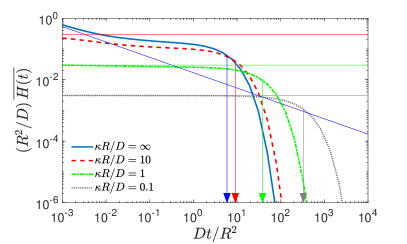
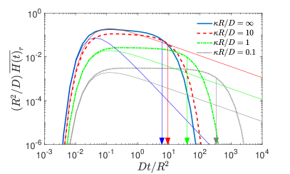
Figure 4: Volume-average (left) and surface-averaged (right) PDFs $\overline{H(t)}$ and $\overline{H(t)}_{r}$ of the first reaction time through a spherical cap, with $R=1$, $r=0.5$, $D=1$, $\varepsilon=0.2$, and several values of $\kappa$. Self-consistent approximation is truncated to $n=100$ terms. Arrows indicate the mean FRT. Thin lines show the short-time asymptotic behaviours (76) and (79) for two plots, respectively.

Finally, the short-time asymptotic behaviour of $H(r,\theta;t)$ is obtained by combining (75) and (77) to get

$$\tilde{H}(r,\theta;p)\simeq\frac{R(1-\cos\varepsilon)}{2r(1+\sqrt{pD}/\kappa)}e^{-(R-r)\sqrt{p/D}}\biggl{(}1+\sum\limits_{n=1}^{\infty}\phi_{n}(\varepsilon)\,P_{n}(\cos\theta)\biggr{)}.$$

The sum in the parentheses can be computed exactly by noting that

$$P_{n-1}(x)-P_{n+1}(x)=\frac{2n+1}{n(n+1)}(1-x^{2})P^{\prime}_{n}(z)=(2n+1)\int\limits_{x}^{1}dx^{\prime}P_{n}(x^{\prime})$$

and using the completeness of the Legendre polynomials:

$$\sum\limits_{n=0}^{\infty}\frac{2n+1}{2}\,P_{n}(x)\,P_{n}(y)=\delta(x-y).$$ (82)

We get thus

$$\tilde{H}(r,\theta;p)\simeq\frac{Re^{-(R-r)\sqrt{p/D}}}{r(1+\sqrt{pD}/\kappa)}\,\Theta(\varepsilon-\theta)\qquad(p\to\infty),$$ (83)

where $\Theta(x)$ is the Heaviside function. The inverse Laplace transform reads

$$H(r,\theta;t)\simeq\frac{R\,\Theta(\varepsilon-\theta)}{r\sqrt{\pi Dt}}e^{-(R-r)^{2}/(4Dt)}\times\left\{\begin{array}[]{l l}\kappa&(\kappa<\infty),\\ (R-r)/(2t)&(\kappa=\infty).\\ \end{array}\right.$$ (84)

The Heaviside function distinguishes two cases. When the starting point lies within the solid angle of the target (i.e., $\theta<\varepsilon$), the distance to the target is just $R-r$, and this asymptotic formula holds. In turn, when the starting point lies outside this solid angle (i.e., $\theta>\varepsilon$), the distance to the target is larger than $R-r$, $\tilde{H}(r,\theta;p)$ should decay faster, the contributions in (83) and (84) are thus cancelled, and one needs more refined asymptotic analysis. Without dwelling further on this analysis, we present below probabilistic arguments to get a reasonable approximation.

When the starting point is far from the small escape window, small exit times are extremely unlikely, with the probability density vanishing exponentially fast as $\exp(-\sigma^{2}/(4Dt))$, where $\sigma\gg\sqrt{Dt}$ is the distance to the escape window. To find the correct prefactor to this exponential tail, we note that (i) a small spherical cap, seen from far away, can approximated by a small sphere of the same radius $\rho=2R\sin(\varepsilon/2)$, centred at the North pole; the distance to the boundary of this sphere is $\sigma=\sqrt{R^{2}+r^{2}-2rR\cos\theta}-\rho$; and (ii) the reflecting boundary of the spherical confining domain can be removed because only almost straight trajectories to the target, not touching the confining boundary, do matter in the short-time limit. In other words, the short-time behaviour of the density $H(r,\theta;t)$ should be close to that of the density $H_{\infty}(\sigma;t)$ for diffusion in the exterior of a small spherical target. The latter was derived by Collins and Kimball [32],

$$H_{\infty}(\sigma;t) = \frac{\kappa}{\sigma+\rho}\exp\biggl{(}-\frac{\sigma^{2}}{4Dt}\biggr{)}\biggl{\{}\frac{\rho}{\sqrt{\pi Dt}}$$ (85)

$$- \biggl{(}1+\frac{\kappa\rho}{D}\biggr{)}\mathrm{erfcx}\biggl{(}\frac{\sigma}{\sqrt{4Dt}}+\biggl{(}1+\frac{\kappa\rho}{D}\biggr{)}\frac{\sqrt{Dt}}{\rho}\biggr{)}\biggr{\}},$$

where $\mathrm{erfcx}(x)=e^{x^{2}}\mathrm{erfc}(x)$ is the scaled complementary error function (see also discussion in [52]). In the limit $\kappa\to\infty$, this expression reduces to

$$H_{\infty}(\sigma;t)=\frac{\rho}{\sigma+\rho}\,\frac{\sigma}{\sqrt{4\pi Dt^{3}}}\,\exp\biggl{(}-\frac{\sigma^{2}}{4Dt}\biggr{)}.$$ (86)

In the limit $\sqrt{Dt}\gg\max\{\sigma,\rho\}$, (85) yields the long-time behaviour in (7).

Figure 5 reproduces the rescaled PDF from Fig. 2 to illustrate the quality of the short-time asymptotic formulae. For the case $\theta=0$, the panel (a) confirms that the short-time asymptotic formula (84) accurately captures the left exponential tail of the PDF up to the most probable time, i.e., for $t\lesssim t_{\rm mp}$. However, this approximation fails at longer times due to the confinement. Note also that the estimation of the most probable time $t_{\rm mp}$ from (84), suggested in [52] for a simpler geometric setting, is not accurate here, except for the perfectly reactive target. From Fig. 5(a), we only can say that $t_{\rm mp}<(R-r)^{2}/(6D)$ for the perfectly reactive target ($\kappa=\infty$), and $t_{\rm mp}<(R-r)^{2}/(2D)$ for partially reactive targets ($\kappa<\infty$). The panels (b) and (c) illustrate the accuracy of another short-time asymptotic formula, given by (85), which is applicable when the starting point is far away from the target ($\theta=\pi/2$ and $\theta=\pi$, respectively). Once again, the left exponential tail of $H(r,\theta;t)$ is captured reasonably well. In this case, there is no hump, and a plateau region emerges immediately after this tail. As the most probable time now belongs to this plateau region, it is very difficult to quantify. This is a radically new feature of the narrow escape problem, as compared to recent works [47, 52].

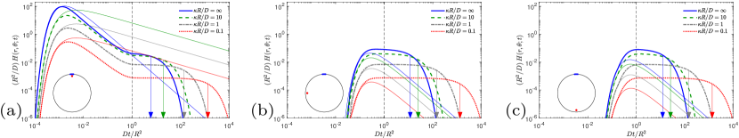
Figure 5: PDF $H(r,\theta;t)$, rescaled by $R^{2}/D$, as shown on Fig. 2, is compared to its short-time approximation (84) for $\theta=0$ (a) and (85) for $\theta=\pi/2$ (b) and $\theta=\pi$ (c), shown by thin lines of the same colour. The other parameters are kept: $r/R=0.9$, $\varepsilon=0.1$, $\bar{\kappa}=\kappa R/D$ as indicated in the panels. Vertical arrows indicate the rescaled mean FRT $Dt_{\rm mean}/R^{2}$, while the dashed vertical line shows the rescaled crossover time $Dt_{c}/R^{2}=1$.

C.3 Explicit closed-form approximation

The knowledge of both short-time and long-time asymptotic behaviours of the probability density motivated the search of closed-form approximations for the probability density $H(r,\theta;t)$ over the whole range of times. For instance, Isaacson and Newby developed a uniform asymptotic approximation for perfectly reactive small targets in bounded domains using a short-time correction calculated by a pseudopotential approximation [54]. In turn, a linear superposition of the short-time approximation in (85) with the long-time exponential decay was proposed in [52] for a partially reactive spherical target located in the centre of a larger confining sphere.

Here, we rationalise and improve the linear superposition by employing the simple idea of splitting trajectories toward a small target into two groups: (i) “direct” trajectories that do not hit the boundary of the confining domain and thus do not “know” about its presence, and (ii) “indirect” trajectories that reach the boundary and thus explore the bounded confining domain until eventual reaction with the target. The statistics of direct trajectories is close to that of trajectories in the unbounded exterior of the target; in particular, if the starting point is far from a small target, the probability density of the first exit (reaction) times is close to $H_{\infty}(\sigma;t)$ given by (85). In turn, the indirect trajectories are responsible for the long-time exponential decay of the probability density. If $\tau_{1}$ and $\tau_{2}$ denote the conditional first exit times for such direct and indirect trajectories respectively, then one can set $\tau=\tau_{1}$ with the probability $q_{1}$ of realising a direct trajectory, and $\tau=\tau_{2}$ with the probability $q_{2}=1-q_{1}$ of realising an indirect trajectory. If the related probability densities $\rho_{1}(t)$ and $\rho_{2}(t)$ were known, then the probability density of $\tau$ would be simply

$$H(r,\theta;t)=q_{1}\rho_{1}(t)+q_{2}\rho_{2}(t).$$ (87)

The computation of the probability densities $\rho_{1}(t)$ and $\rho_{2}(t)$ is an even more complicated problem than the original mixed boundary problem for $H(r,\theta;t)$. So, we propose another, much simpler splitting into two groups by introducing a heuristic threshold $T$ for the first exit time. In this approximation, all trajectories toward the target that are shorter than $T$ are treated as “direct”, whereas all longer trajectories are treated as “indirect”. According to this construction, the first exit times of direct trajectories, that can be described by the probability density $H_{\infty}(\sigma;t)$, are conditioned to be shorter than $T$; in turn, the first exit times of indirect trajectories, that can be described by the probability density $\mu e^{-\mu t}$ with $\mu=D\lambda_{0}$ being related to the smallest eigenvalue $\lambda_{0}$ of the Laplace operator in the confining domain, are conditioned to be longer than $T$. The related conditional probability densities are then given as

$$\rho_{1}(t) = \Theta(T-t)H_{\infty}(\sigma;t)/(1-S_{\infty}(\sigma;T)),$$ (88a)

$$\rho_{2}(t) = \Theta(t-T)\mu e^{-\mu(t-T)},$$ (88b)

where

$$S_{\infty}(\sigma;t) = 1-\frac{\rho\exp\bigl{(}-\frac{\sigma^{2}}{4Dt}\bigr{)}}{(\sigma+\rho)(1+D/(\kappa\rho))}\biggl{\{}\mathrm{erfcx}\biggl{(}\frac{\sigma}{\sqrt{4Dt}}\biggr{)}$$ (89)

$$- \mathrm{erfcx}\biggl{(}\frac{\sigma}{\sqrt{4Dt}}+\left(1+\frac{\kappa\rho}{D}\right)\frac{\sqrt{Dt}}{\rho}\biggr{)}\biggr{\}}$$

is the survival probability obtained by integrating $H_{\infty}(\sigma;t)$. To ensure the continuity of $\rho(t)$ in (87), we set

$$q_{1}=\frac{\mu e^{-\mu T}(1-S_{\infty}(\sigma;T))}{H_{\infty}(\sigma;T)e^{-\mu T}+\mu e^{-\mu T}(1-S_{\infty}(\sigma;T))}\,.$$ (90)

The threshold $T$ can either be fixed to a prescribed value (e.g., $T=t_{c}$), or determined by imposing an additional condition, i.e., the continuity of the derivative of $\rho(t)$. Figure 6 illustrates the accuracy of this explicit approximation.

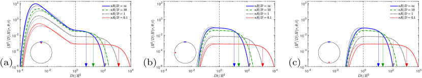
Figure 6: PDF $H(r,\theta;t)$, rescaled by $R^{2}/D$, as shown on Fig. 2, is compared to the approximation in (87) for $\theta=0$ (a), $\theta=\pi/2$ (b) and $\theta=\pi$ (c), shown by thin lines of the same colour. The other parameters are kept: $r/R=0.9$, $\varepsilon=0.1$, $\bar{\kappa}=\kappa R/D$ as indicated in the panels. Vertical arrows indicate the mean FRT $t_{\rm mean}$, while the dashed vertical line shows the crossover time $t_{c}=R^{2}/D$. We set $T=0.5t_{c}$.

Appendix D Basic properties and implementation

The functions $g_{n}$ and their derivatives can be computed via the recurrent relations

$$g_{0}(r) = \frac{\sinh\xi}{\xi}\,,\qquad g_{1}(r)=\frac{\xi\cosh\xi-\sinh\xi}{\xi^{2}}\,,$$ (91)

$$g_{n+1}(r) = g_{n-1}(r)-\frac{2n+1}{\xi}g_{n}(r)\quad(n=1,2,\ldots),$$ (92)

$$g^{\prime}_{0}(r) = \sqrt{p/D}\,g_{1}(r),$$ (93)

$$g^{\prime}_{n}(r) = \sqrt{p/D}\biggl{(}g_{n-1}(r)-\frac{n+1}{\xi}g_{n}(r)\biggr{)},$$ (94)

with $\xi=r\sqrt{p/D}$. As a consequence, one has

$$r\frac{g^{\prime}_{0}(r)}{g_{0}(r)} = r\sqrt{p/D}\,\frac{g_{1}(r)}{g_{0}(r)}=\frac{\xi^{2}}{f_{1}}\,,$$ (95)

$$r\frac{g^{\prime}_{n}(r)}{g_{n}(r)} = f_{n}-(n+1)\quad(n=1,2,\ldots),$$ (96)

where new functions

$$f_{n}=\xi\,\frac{g_{n-1}(r)}{g_{n}(r)}$$ (97)

satisfy the recurrent relations

$$f_{1} = \frac{\xi^{2}}{\xi\coth\xi-1}\,,$$ (98)

$$f_{n} = \frac{\xi^{2}}{f_{n-1}-(2n-1)}\quad(n=2,3,\ldots).$$ (99)

Unfortunately, these relations are numerically unstable for $\xi$ below $n$ that prohibits their use even for moderate $n$.

In order to resolve this numerical problem, we propose the following trick. Rewriting (99) as

$$f_{n}=2n+1+\frac{\xi^{2}}{f_{n+1}}\,,$$ (100)

one can consider the recurrent relations for $f_{n}$ as a continued fraction representation:

$$\xi\coth\xi=1+\frac{\xi^{2}}{\displaystyle 3+\frac{\xi^{2}}{\displaystyle 5+\frac{\xi^{2}}{7+\cdots}}}\,.$$ (101)

To overcome numerical instabilities, we propose the following algorithm: (i) for any $\xi$, we select a large enough truncation parameter $n_{\rm max}$ such that $n_{\rm max}\gg|\xi|$ (in practice, we set $n_{\rm max}=\max\{100,[10\xi]\}$); (ii) we approximate $f_{n}$ with $n=n_{\rm max}$ according to its Taylor expansion

$$f_{n} = 2n+1+\frac{\xi^{2}}{2n+3}-\frac{\xi^{4}}{(2n+3)^{2}(2n+5)}+\frac{2\xi^{6}}{(2n+3)^{3}(2n+5)(2n+7)}$$

$$- \frac{(10n+27)\xi^{8}}{(2n+3)^{4}(2n+5)^{2}(2n+7)(2n+9)}+O(\xi^{10}),$$

which is valid whenever $|\xi|\ll n$ (even if $|\xi|$ is large); (iii) applying (100) in a backward direction, we compute all $f_{n}$ with $1\leq n\leq n_{\rm max}$. When the argument $|\xi|$ is very large (as compared to $n$), one can use the asymptotic relation

$$f_{n}=\xi+n+\frac{n(n+1)}{2\xi}+O(\xi^{-2})\qquad(\xi\to\infty).$$ (103)

We checked that this algorithm provides very accurate results for real $\xi$. Qualitatively, the improved numerical stability of recurrent relations in the backward direction resembles the advantage of an implicit Euler scheme for solving differential equations over an explicit one. Note that the computation can be more subtle for some imaginary $\xi$, at which $\coth\xi$ diverges (i.e., at $\xi=i\pi k$ with an integer $k$). However, we have not experienced such numerical difficulties for considered parameters.

We note that (96) and (D) imply

$$r\frac{g^{\prime}_{n}(r)}{g_{n}(r)}=n+\frac{\xi^{2}}{2n+3}-\frac{\xi^{4}}{(2n+3)^{2}(2n+5)}+O(\xi^{6}),$$ (104)

which could also be obtained directly from

$$g_{n}(r)=\frac{\sqrt{\pi}}{2}\sum\limits_{k=0}^{\infty}\frac{(z/2)^{n+2k}}{k!\,\Gamma(n+k+1/2)}$$ (105)

(with $z=r\sqrt{p/D}$). One sees that for $z\geq 0$, all functions $g_{n}(r)$ are positive and monotonously increasing because

$$g^{\prime}_{n}(r)=\sqrt{p/D}\biggl{(}\frac{n}{2n+1}g_{n-1}(r)+\frac{n+1}{2n+1}g_{n+1}(r)\biggr{)}\geq 0.$$ (106)

We also define $\hat{f}_{n}(\xi)=f_{n}(i\xi)$ so that

$$\frac{Rg^{\prime}_{0}(R)}{g_{0}(R)}=-\frac{\alpha^{2}}{\hat{f}_{1}}\,,\quad\frac{Rg^{\prime}_{n}(R)}{g_{n}(R)}=\hat{f}_{n}-(n+1),$$ (107)

with $\hat{f}_{n}(\alpha)=\alpha\,j_{n-1}(\alpha)/j_{n}(\alpha)$ for $n=1,2,3,\ldots$, which yields

$$\hat{f}_{1}=\frac{\alpha^{2}}{1-\alpha\,\mathrm{ctan}\alpha}\,,\qquad\hat{f}_{n}=\frac{\alpha^{2}}{2n-1-\hat{f}_{n-1}}\,.$$ (108)

In particular, one gets

$$F(\alpha)=-\frac{\hat{f}_{1}(\alpha)}{\alpha^{2}}+\sum\limits_{n=1}^{\infty}\frac{\phi_{n}^{2}(\varepsilon)}{2n+1}\,\frac{1}{\hat{f}_{n}(\alpha)-(n+1)}\,.$$ (109)

Note that these recurrent relations yield very accurate results for $\alpha\gtrsim n$. For smaller $\alpha$, one can use the Taylor expansion of $\hat{f}_{n}$.

Appendix E Numerical verification

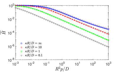
Figure 7: Volume-averaged Laplace-transformed PDF $\overline{\tilde{H}(p)}$ of the FRT through a spherical cap, with $R=1$, $D=1$, $\varepsilon=0.1$ (left) and $\varepsilon=1$ (right), and several values of $\kappa$. Self-consistent approximation (lines), truncated to $n=1000$ terms, is compared to the FEM solution of the original problem (symbols), with $h_{\rm max}=0.01$. Note that our theoretical predictions are almost indistinguishable from the FEM solution for several decades of variation of the dimensionless parameter $R^{2}p/D$.

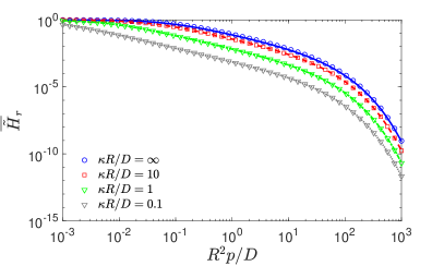
Figure 8: Surface-averaged Laplace-transformed PDF $\overline{\tilde{H}(p)}_{r}$ of the FRT through a spherical cap, with $R=1$, $D=1$, $r=0.5$, $\varepsilon=0.1$ (left) and $\varepsilon=1$ (right), and several values of $\kappa$. Self-consistent approximation (lines), truncated to $n=1000$ terms, is compared to the FEM solution of the original problem (symbols), with $h_{\rm max}=0.01$. Note that our theoretical predictions are almost indistinguishable from the FEM solution for several decades of variation of the dimensionless parameter $R^{2}p/D$.

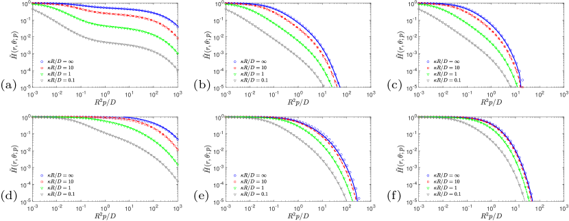
Figure 9: Laplace-transformed PDF $\tilde{H}(r,\theta;p)$ of the FRT through a spherical cap, with $R=1$, $D=1$, $r=0.9$, $\varepsilon=0.1$ (top panels) and $\varepsilon=1$ (bottom panels), four values of $\kappa$, and (a,d) $\theta=0$, (b,e) $\theta=\pi/2$, (c,f) $\theta=\pi$ (these starting points correspond to those used in figures 2, 5 and 6). The self-consistent approximation (lines), truncated to $n=50$ terms, is compared to the FEM solution of the original problem (symbols), with $h_{\rm max}=0.01$. Note that our theoretical predictions are almost indistinguishable from the FEM solution for several decades of variation of the dimensionless parameter $R^{2}p/D$.

In order to assess the accuracy of the self-consistent approximation, we solve numerically the original boundary value problem for the modified Helmholtz equation

$$(p-D\Delta)\tilde{H}(r,\theta;p)=0,$$ (110)

subject to the mixed boundary condition:

$$\frac{D}{\kappa}\partial_{n}\tilde{H}+\tilde{H} = 1\quad(0\leq\theta<\varepsilon),$$ (111)

$$\partial_{n}\tilde{H} = 0\quad(\varepsilon\leq\theta\leq\pi).$$ (112)

Setting $u(\rho,\theta;s)=\tilde{H}(\rho R,\theta;p)$ with rescaled radial coordinate $\rho=r/R$, this equation can be written in spherical coordinates as

$$\partial_{\rho}\rho^{2}\sin\theta\partial_{\rho}u+\partial_{\theta}\sin\theta\partial_{\theta}u-s\rho^{2}\sin\theta u=0,$$ (113)

where $s=pR^{2}/D$ and we omitted the azimuthal angle due to the axial symmetry of the problem. We solve the above equation on the planar computational domain $C=(0,1)\times(0,\pi)$ by using a Finite Elements Method (FEM) implemented as PDE toolbox in Matlab. For this purpose, we rewrite this equation in the conventional matrix form:

$$-\left(\begin{array}[]{c}\partial_{\rho}\\ \partial_{\theta}\\ \end{array}\right)^{\dagger}c\left(\begin{array}[]{c}\partial_{\rho}\\ \partial_{\theta}\\ \end{array}\right)u+au=0,$$ (114)

where $c$ is the diagonal $2\times 2$ matrix with elements $\rho^{2}\sin\theta$ and $\sin\theta$, and $a=s\rho^{2}\sin\theta$. This equation is to be solved subject to the boundary conditions:

$$(\partial_{\rho}u)_{\rho=0}=(\partial_{\theta}u)_{\theta=0}=(\partial_{\theta}u)_{\theta=\pi}=0,$$ (115)

$$\frac{D}{\kappa R}(\partial_{\rho}u)_{\rho=1}+u_{\rho=1}=1\quad(0\leq\theta<\varepsilon),$$ (116)

$$(\partial_{\rho}u)_{\rho=1}=0\quad(\varepsilon\leq\theta\leq\pi).$$ (117)

Once the solution is found, we also evaluate the volume average $\overline{\tilde{H}(p)}$ (by numerical integration over the triangular mesh), and the surface average $\overline{\tilde{H}(p)}_{r}$ (by interpolating the solution to a line $\rho=const$ and then integrating numerically over $\theta$). We selected the maximal mesh size to be $h_{\rm max}=0.01$. In order to verify the accuracy of the FEM solution, we solved the problem twice, with two mesh sizes $h_{\rm max}$ and $2h_{\rm max}$, and checked that the resulting solutions were barely distinguishable.

Figures 7 and 8 compare the volume-averaged and surface-averaged Laplace-transformed PDFs $\overline{\tilde{H}(p)}$ and $\overline{\tilde{H}(p)}_{r}$, obtained via our self-consistent approximation (lines) and by FEM (symbols). One can see that the self-consistent approximation is remarkably accurate over a broad range of $p$, for both narrow $\varepsilon=0.1$ and extended $\varepsilon=1$ target region. The accuracy is higher for less reactive targets.

Figure 9 compares the Laplace-transformed PDF $\tilde{H}(r,\theta;p)$, obtained via our self-consistent approximation (lines) and by FEM (symbols), for the three starting points used in figures 2, 5 and 6. One can see that the self-consistent approximation is remarkably accurate over a broad range of $p$, for both narrow $\varepsilon=0.1$ and extended $\varepsilon=1$ target region. The accuracy is higher for less reactive targets. Minor deviations seen in panel (c) for the case $\kappa=\infty$ are caused by the truncation to $n=50$ terms and can be corrected by increasing $n$ (not shown). In turn, minor deviations in panel (e) cannot be corrected by increasing $n$ and can thus be attributed to a limited accuracy of the self-consistent approximation for extended targets.

References

- [1] Bressloff PC, Newby JM (2013) Stochastic models of intracellular transport. Rev. Mod. Phys. 85:135-196.
- [2] Holcman D, Schuss Z (2014) The Narrow Escape Problem. SIAM Rev. 56:213-257.
- [3] Redner S (2001) A Guide to First Passage Processes (Cambridge, Cambridge University press).
- [4] Grebenkov DS, Oshanin G (2017) Diffusive escape through a narrow opening: new insights into a classic problem. Phys. Chem. Chem. Phys. 19:2723-2739.
- [5] Grigoriev IV, Makhnovskii YA, Berezhkovskii AM, Zitserman VY (2002) Kinetics of escape through a small hole. J. Chem. Phys. 116:9574-9577.
- [6] Metzler R, Oshanin G, Redner S (2014) First-Passage Phenomena and Their Applications (Singapore, World Scientific).
- [7] Bénichou O, Voituriez R (2014) From first-passage times of random walks in confinement to geometry-controlled kinetics. Phys. Rep. 539:225-284.
- [8] Rayleigh JWS (1945) The Theory of Sound. Vol. 2, 2nd Ed. (Dover, New York).
- [9] Holcman D, Schuss Z (2004) Escape Through a Small Opening: Receptor Trafficking in a Synaptic Membrane. J. Stat. Phys. 117:975-1014.
- [10] Singer A, Schuss Z, Holcman D, Eisenberg RS (2006) Narrow Escape, Part I. J. Stat. Phys. 122:437-463.
- [11] Schuss Z, Singer A, Holcman D (2007) The narrow escape problem for diffusion in cellular microdomains. Proc. Nat. Acad. Sci. USA 104:16098-16103.
- [12] Cheviakov AF, Ward MJ, Straube R (2010) An Asymptotic Analysis of the Mean First Passage Time for Narrow Escape Problems: Part II: The Sphere. SIAM Multi. Model. Simul. 8:836-870.
- [13] Bénichou O, Voituriez R. (2008) Narrow-Escape Time Problem: Time Needed for a Particle to Exit a Confining Domain through a Small Window. Phys. Rev. Lett. 100:168105.
- [14] Caginalp C, Chen X (2012) Analytical and Numerical Results for an Escape Problem. Arch. Rational. Mech. Anal. 203: 329-342.
- [15] Singer A, Schuss Z, Holcman D (2006) Narrow Escape, Part III Riemann surfaces and non-smooth domains. J. Stat. Phys. 122: 491-509.
- [16] Pillay S, Ward MJ, Peirce A, Kolokolnikov T (2010) An Asymptotic Analysis of the Mean First Passage Time for Narrow Escape Problems: Part I: Two-Dimensional Domains. SIAM Multi. Model. Simul. 8: 803-835.
- [17] Cheviakov AF, Reimer AS, Ward MJ (2012) Mathematical modeling and numerical computation of narrow escape problems. Phys. Rev. E 85:021131.
- [18] Grebenkov DS (2016) Universal formula for the mean first passage time in planar domains. Phys. Rev. Lett. 117:260201.
- [19] Grebenkov DS, Traytak S (2019) Semi-analytical computation of Laplacian Green functions in three-dimensional domains with disconnected spherical boundaries. J. Comput. Phys. 379: 91-117.
- [20] Holcman D, Schuss Z (2012) Brownian Motion in Dire Straits. SIAM Multiscale Mod. Sim. 10:1204-1231.
- [21] Oshanin G, Tamm M, Vasilyev O (2010) Narrow-escape times for diffusion in microdomains with a particle-surface affinity: Mean-field results. J. Chem. Phys. 132:235101.
- [22] Bénichou O, Grebenkov DS, Levitz P, Loverdo C, Voituriez R (2010) Optimal Reaction Time for Surface-Mediated Diffusion. Phys. Rev. Lett. 105:150606.
- [23] Bénichou O, Grebenkov DS, Levitz P, Loverdo C, and Voituriez R (2011) Mean first-passage time of surface-mediated diffusion in spherical domains. J. Stat. Phys. 142:657-685.
- [24] Rupprecht J-F, Bénichou O, Grebenkov DS, Voituriez R (2012) Kinetics of active surface-mediated diffusion in spherically symmetric domains. J. Stat. Phys. 147:891-918.
- [25] Berezhkovskii AM, Barzykin AV (2012) Search for a Small Hole in a Cavity Wall by Intermittent Bulk and Surface Diffusion. J. Chem. Phys. 136: 054115.
- [26] Berezhkovskii AM, Dagdug L (2012) Effect of Binding on Escape from Cavity through Narrow Tunnel. J. Chem. Phys. 136: 124110.
- [27] Agranov T, Meerson B (2018) Narrow Escape of Interacting Diffusing Particles. Phys. Rev. Lett. 120:120601.
- [28] Lanoiselée Y, Moutal N, Grebenkov DS (2018) Diffusion-limited reactions in dynamic heterogeneous media. Nature Commun. 9:4398.
- [29] Rojo F, Wio HS, Budde CE (2012) Narrow-escape-time problem: The imperfect trapping case. Phys. Rev. E 86:031105.
- [30] Grebenkov DS, Metzler R, Oshanin G (2017) Effects of the target aspect ratio and intrinsic reactivity onto diffusive search in bounded domains. New J. Phys. 19:103025.
- [31] Grebenkov DS, Metzler R, Oshanin G, Dagdug L, Berezhkovskii AM, Skvortsov AT (2019) Trapping of diffusing particles by periodic absorbing rings on a cylindrical tube. J. Chem. Phys. 150:206101.
- [32] Collins FC, Kimball GE (1949) Diffusion-controlled reaction rates. J. Colloid Sci. 4:425-437.
- [33] Rupprecht J-F, Bénichou O, Grebenkov DS, Voituriez R (2015) Exit time distribution in spherically symmetric two-dimensional domains. J. Stat. Phys. 158:192-230.
- [34] Hafner AE, Rieger H (2018) Spatial cytoskeleton organization supports targeted intracellular transport. Biophys. J. 114:1420-1432.
- [35] Mattos T, Mejía-Monasterio C, Metzler R, Oshanin G (2012) First passages in bounded domains: When is the mean first passage time meaningful? Phys. Rev. E 86:031143.
- [36] Mejía-Monasterio C, Oshanin G, Schehr G (2011) First passages for a search by a swarm of independent random searchers. J. Stat. Mech. P06022.
- [37] Godec A, Metzler R (2016) First passage time distribution in heterogeneity controlled kinetics: going beyond the mean first passage time. Sci. Rep. 6:20349.
- [38] He Y, Burov S, Metzler R, Barkai E (2008) Random Time-Scale Invariant Diffusion and Transport Coefficients. Phys. Rev. Lett. 101: 058101.
- [39] Schulz JHP, Barkai E, Metzler R (2014) Aging renewal theory and application to random walks. Phys. Rev. X 4:011028.
- [40] Krapf D, Marinari E, Metzler R, Oshanin G, Squarcini A, Xu X (2018) Power spectral density of a single Brownian trajectory: What one can and cannot learn from it. New J. Phys. 20:023029.
- [41] Krapf D, Lukat N, Marinari E, Metzler R, Oshanin G, Selhuber-Unkel C, Squarcini A, Stadler L, Weiss M, Xu X (2019) Spectral Content of a Single Non-Brownian Trajectory. Phys. Rev. X 9:011019.
- [42] Sposini V, Metzler R, Oshanin G (2019) Single-trajectory spectral analysis of scaled Brownian motion. New J. Phys. 21:073043.
- [43] Yu J, Xiao J, Ren X, Lao K, Xie XS (2006) Probing gene expression in live cells, one protein molecular at a time. Science 311:1600.
- [44] Mugler A, Tostevin F, ten Wolde PR (2013) Spatial partitioning improves the reliability of biochemical signaling. Proc. Natl. Acad. Sci. USA 110: 5927-5932.
- [45] Cebecauer M, Spitaler M, Sergé A, Magee AI (2010) Signalling complexes and clusters: functional advantages and methodological hurdles. J. Cell Sci. 123:309-320.
- [46] Shoup D, Lipari G, Szabo A (1981) Diffusion-controlled bimolecular reaction rates. The effect of rotational diffusion and orientation constraints. Biophys. J. 36:697-714.
- [47] Grebenkov DS, Metzler R, Oshanin G (2018) Towards a full quantitative description of single-molecule reaction kinetics in biological cells. Phys. Chem. Chem. Phys. 20:16393-16401.
- [48] Grebenkov DS (2019) Imperfect Diffusion-Controlled Reactions, in “Chemical Kinetics Beyond the Textbook”, Eds. R. Metzler, K. Lindenberg, G. Oshanin (World Scientific, 2019) [Available online: ArXiv 1806.11471].
- [49] Oshanin G, Popescu M N, Dietrich S (2017) Active colloids in the context of chemical kinetics. J. Phys. A: Math. Theor. 50:134001.
- [50] Grebenkov DS (2019) Spectral theory of imperfect diffusion-controlled reactions on heterogeneous catalytic surfaces. J. Chem. Phys. 151:104108.
- [51] Godec A, Metzler R (2016) Universal proximity effect in target search kinetics in the few encounter limit. Phys. Rev. X 6:041037.
- [52] Grebenkov DS, Metzler R, Oshanin G (2018) Strong defocusing of molecular reaction times results from an interplay of geometry and reaction control. Commun. Chem. 1:96.
- [53] Ward MJ, Keller JB (1993) Strong Localized Perturbations of Eigenvalue Problems. SIAM J. Appl. Math. 53:770-798.
- [54] Isaacson SA, Newby J (2013) Uniform asymptotic approximation of diffusion to a small target. Phys. Rev. E 88:012820.
- [55] Grebenkov DS, Nguyen B-T (2013) Geometrical structure of Laplacian eigenfunctions. SIAM Rev. 55:601-667.
- [56] Zwanzig, R (1992) Diffusion past an entropy barrier. J. Phys. Chem. 96:3926.
- [57] Berezhkovskii AM, Zitserman VYu, Shvartsman SY (2003) Diffusivity in Periodic Arrays of Spherical Cavities. J. Chem. Phys. 118:7146.
- [58] Reguera D, Schmid G, Burada PS, Rubí JM, Reimann P, Hänggi P (2006) Entropic Transport: Kinetics, Scaling, and Control Mechanisms. Phys. Rev. Lett. 96:130603.
- [59] Berezhkovskii AM, Pustovoit MA and Bezrukov SM (2009) Entropic Effects in Channel-Facilitated Transport: Inter-Particle Interactions Break the Flux Symmetry. Phys. Rev. E 80:020904(R)
- [60] Malgaretti P, Pagonabarraga I, Rubí JM (2013) Confined Brownian ratchets. J. Chem. Phys. 138:194906.
- [61] Berezhkovskii AM, Makhnovskii YuA, Zitserman VYu (2006) Escape from a Cavity through a Small Window: Turnover of the Rate as a Function of Friction Constant. J. Chem. Phys. 125:194501.
- [62] Berezhkovskii AM, Barzykin AV, Zitserman VYu (2009) Escape from Cavity through Narrow Tunnel. J. Chem. Phys. 130:245104.
- [63] Cheng K L, Sheng Y J, Tsao H-K (2008) Brownian escape and force-driven transport through entropic barriers. J. Chem. Phys. 129:184901.
- [64] Holcman D, Schuss Z (2012) Brownian needle in dire straits: Stochastic motion of a rod in very confined narrow domains. Phys. Rev. E 85:010103(R).
- [65] Malgaretti P, Pagonabarraga I, Rubí JM (2012) Cooperative rectification in confined Brownian ratchets. Phys. Rev. E 85:010105(R).
- [66] Schuss Z, Basnayake K, Holcman D (2019) Redundancy principle and the role of extreme statistics in molecular and cellular biology. Phys. Life Rev. 28:52-79.
- [67] Di Rienzo C, Piazza V, Gratton E, Beltram F, Cardarelly F (2014) Probing short-rangle protein Brownian motion in the cytoplasm of living cells. Nature Comm. 5:5891.
- [68] Loffreda A, Jacchetti E, Antunes S, Rainone P, Daniele T, Morisaki T, Bianchi ME, Tacchetti C, Mazza D (2017) Live-cell p53 single-molecule binding is modulated by C-terminal acetylation and correlates with transcriptional activity. Nature Comm. 8:313.
- [69] Gebhardt JCM, Suter DM, Roy R, Zhao ZW, Chapman AR, Basu S, Maniatis T, Xie XS (2013) Single molecule imaging of transcription factor binding to DNA in live mammalian cells. Nature Methods 10:421.
- [70] Elf J, Barkefors I (2019) Single-molecule kinetics in living cells. Ann. Rev. Biochem. 88:635-659
- [71] Kolesov G, Wunderlich Z, Laikova ON, Gelfand MS, Mirny LA (2007) How gene order is influenced by the biophysics of transcription regulation. Proc. Natl. Acad. Sci. USA 104:13948-13953.
- [72] Pulkkinen O, Metzler R (2013) Distance matters: the impact of gene proximity in bacterial gene regulation. Phys. Rev. Lett. 110:198101.
- [73] Karlsson A, Karlsson R, Karlsson M, Cans ASS, Stromberg A, Ryttsen F, Orwar O (2001) Molecular engineering: Networks of nanotubes and containers. Nature 409:150-152.