Emergence of prethermal states in a driven dissipative system through cross-correlated dissipation

Abstract

Periodically driven closed quantum many-body systems are known to exhibit prethermal or quasi-steady-state dynamics. In this work, we theoretically show that such prethermal phases can appear in the dynamics of a dipolar two-spin-$1/2$ system coupled to a heat bath if the cross terms between the drive and dipolar interactions are taken into consideration. To this end, we use our recently-reported fluctuation-regulated quantum master equation [A. Chakrabarti and R. Bhattacharyya, Phys. Rev. A 97, 063837 (2018)], to show that the predicted dynamics can successfully explain the experimentally observed features of the transient and prethermal regime.

I Introduction

Periodically driven quantum systems appear in a large class of problems of interest and, therefore, are the subject of continued investigation eckardt17 ; fleckenstein21 ; beatrez21 ; dalessio14 ; sen21 . Theoretical and experimental endeavors have proved that there exist three different regimes in the dynamics of periodically driven quantum ensembles, v.i.z. i) a transient phase, ii) a prethermal quasi-steady state, and iii) unconstrained thermalization when the drive amplitude or the Rabi frequency is sufficiently high beatrez21 ; santos21 . Similar dynamical features in the presence of drives having lower amplitudes have also been predicted fleckenstein21 . The emergence of the prethermal quasi-steady state is of particular importance, which can be used for engineering quantum gates, preserving coherences (and hence quantum information), and understanding the physics of thermalization processes in general goldman14 ; bukov15 ; singh19 . Most of the theoretical framework developed in this regard concerns closed quantum ensembles whereby unconstrained thermalization results from the breakdown of a Floquet-Magnus approximation used to describe the transient and prethermal dynamics dalessio14 . Only recently, the emergence of a prethermal quasi-steady state has been predicted by Anglés-Castillo et al. for a two-level system, coupled in cascade to two distinct thermal reservoirs, with different equilibrium temperatures castillo20 . The quasi-stable prethermal state observed therein is due to local thermalization induced by the reservoir to which the system is directly coupled, while the final nonequilibrium steady state corresponds to global equilibration castillo20 . It is then pertinent to ask whether prethermal states can also be observed in multi-partite open quantum systems that are directly coupled to a thermal bath?

In this context, it is interesting to note that a quantum system comprising interacting sub-parts, coupled to a single external bath (source of decoherence), can have additional immunity to decoherence grigorenko05 . Moreover, it has already been demonstrated that the cooperative dynamics of two interacting (dipole-dipole) two-level atoms can result in the inhibition of their fluorescence – a phenomenon attributed to the coupling between the symmetric and antisymmetric collective states lawande90 . The emergence of collective steady-states of driven two-level systems coupled by their mutual dipolar interactions has received considerable interest in the recent years parmee17 ; parmee18 ; parmee20 ; landa20 . In this work, our aim is to show that the prethermal phase can also appear in the dynamics of an interacting two-qubit system, coupled to a thermal bath if we consider the cross-correlated dissipators from the drive and inter-qubit interactions. Such prethermal states are essentially quasi-stable collective coherences, which emerge due to their relative immunity to some of the decay channels.

The standard techniques for treating open quantum dynamics cannot be adopted to account for the interplay of drive and inter-qubit interaction, which we wish to capture. But, our recently-proposed Fluctuation Regulated Quantum Master Equation (FRQME), which derives all second-order terms with an explicit regulator originating from the average effect of thermal fluctuations in the environment, can offer a probable solution chakrabarti2018b . Through the second-order terms of a coherent drive, FRQME predicts the presence of a unique drive-dependent decay rate, which has been experimentally observed by the authors in a single spin ensemble chakrabarti2018b ; chakrabarti2018a . Motivated by this success, in the present work, we use FRQME to describe the dissipative dynamics of a driven two-spin-$1/2$ system having dipolar interactions. Interestingly, the drive-dependence of thermalization rates has recently been reported for periodically driven closed quantum many-body systems which show prethermal phases in their dynamics fleckenstein21 .

To focus mainly on the effect of drive-dipole cross-terms in the second order, we shall assume a weak system-environment coupling – weaker than both the drive and dipolar interaction. The equations of motion obtained from this exercise suggest that an initially created collective coherence will be persistent. In practice, the predicted persistent coherence will decay due to the system-environment coupling, indicating the transition to complete thermalization. The quasi-steady-state coherences are akin to the spin-locked magnetization often encountered in magnetic resonance.

The manuscript is organized in the following order: in the next section, we briefly describe the FRQME, pointing out its key features. We then apply this FRQME to a driven two-spin-$1/2$ system, coupled by their mutual dipolar interactions, whereby we obtain drive-dipole cross-terms in the dissipator. In the following section, we present the relevant macroscopic dynamical equations to describe the observed phenomena. The solution of these dynamical equations illustrates the emergence of the collective steady-state coherence and can account for previously observed experimental results, unlike other theoretical approaches. We end with a discussion on the method and the results obtained and a short conclusion highlighting the implications and probable applications of this approach.

II Fluctuation-regulated quantum master equation

One of the major motivations of our alternate formulation of the quantum master equation was to include the higher-order effects of external drives in the dynamics. Such higher-order effects influence the dynamics through well-studied shift terms (such as, light shifts and Bloch-Siegert shifts), and relatively less explored drive-induced dissipation terms chatterjee2020 ; chakrabarti2018a ; chanda2020 ; chanda2021 . Since the complete derivation and the essential features of FRQME have been presented elsewhere chakrabarti2018b , here we present a brief review of its framework. The basic premises of a standard Markovian QME including the Born and Markov approximations, are used in our formulation of FRQME. In addition to those, we also take into account an additional process in the form of an explicit Hamiltonian which strives to capture the ubiquitous thermal fluctuations in the bath. Specifically, we formulate our problem for a quantum system (ensemble) that is interacting with a thermal bath. Each member of the system ensemble (each $2$-spin unit in our case) is directly coupled to a finite portion of the bath, which we name as the “local environment”. For example, in a dilute spin-ensemble (as in beatrez21 ), each spin unit ($2$-spin unit in our case) is directly coupled to the spatial degrees of freedom of molecules in its immediate vicinity. The collection of all these local environments form the bath, which is in thermal equilibrium. The time-independent equilibrium density matrix of the bath is obtained from an ensemble average of the local-environment density matrices. Individual local environments must always experience equilibrium thermal fluctuations in order to ensure that there is no average coherence build-up in the bath, even though evolution under system-local environment interaction takes place.

So, for a system weakly-coupled to its local environment, the full Hamiltonian of each ensemble member (system + local environment), in units of angular frequency, is given by

$$\mathscr{H}(t)=\mathscr{H}_{S}^{\circ}+\mathscr{H}_{L}^{\circ}+\mathscr{H}_{SL}+\mathscr{H}_{\rm sys}(t)+\mathscr{H}_{L}(t),$$ (1)

where, $\mathscr{H}_{S}^{\circ}$ and $\mathscr{H}_{L}^{\circ}$ denote the bare Hamiltonians of the system and the local environment, respectively. $\mathscr{H}_{SL}$ is the coupling between the system and its local environment while $\mathscr{H}_{\rm sys}(t)$ includes all other terms affecting the system alone (e.g. drive, inter-spin interactions in spin networks etc.). Thus, $\mathscr{H}_{\rm sys}(t)$ is assumed to be time-dependent in general. The explicitly time-dependent term $\mathscr{H}_{L}(t)$ represents the fluctuations in the local environments. The collection of these local environments constitute the heat bath, which is assumed to be in thermal equilibrium at an inverse temperature $\beta$, while its energy levels are defined by $\mathscr{H}_{L}^{\circ}$. Since, thermal fluctuations should not destroy the equilibrium populations of the energy levels, $\mathscr{H}_{L}(t)$ is chosen to be diagonal in the eigen-basis $\{|\phi_{j}\rangle\}$ of $\mathscr{H}_{L}^{\circ}$: $\mathscr{H}_{L}(t)=\sum\limits_{j}f_{j}(t)|\phi_{j}\rangle\langle\phi_{j}|$, where, $f_{j}(t)$-s are modeled as independent, Gaussian, $\delta$-correlated stochastic variables with zero mean and standard deviation $\kappa$ i.e. $\overline{f_{j}(t)}=0$ and $\overline{f_{j}(t_{1})f_{k}(t_{2})}=\kappa^{2}\delta_{jk}\delta(t_{1}-t_{2})$ (the overhead line denotes ensemble averaging). Thus, $\mathscr{H}_{L}(t)$ describes equilibrium fluctuations in individual local environments and it has been constructed in such a way that the thermal density matrix remains time-independent as required for sustained equilibrium.

The derivation of FRQME relies on a time coarse-graining method in the interaction representation of $\mathscr{H}_{S}^{\circ}+\mathscr{H}_{L}^{\circ}$, adequately outlined by Cohen-Tannoudji et al.cotandurogryn04 ; chakrabarti2018b , in order to smoothen out the instantaneous effects of the fluctuations while retaining its average effect in the dynamics. Defining $H_{\rm eff}(t):=H_{\rm sys}(t)+H_{SL}(t)$, where the symbol $H$ with relevant subscripts denote the corresponding Hamiltonians in the interaction representation, and $\rho_{S}(t)$ as the reduced density matrix of the system under study, the FRQME is given by chakrabarti2018b :

$$\frac{d}{dt}\rho_{\rm S}(t) = -i\;{\rm Tr}_{\rm L}\!\Big{[}H_{\rm eff}(t),\,\rho_{\rm S}(t)\otimes\rho_{\rm L}^{\rm eq}\Big{]}^{\rm sec}$$ (2)

$$-\int_{0}^{\infty}\kern-11.0ptd\tau\;{\rm Tr}_{\rm L}\!\Big{[}H_{\rm eff}(t),\,\Big{[}H_{\rm eff}(t-\tau),$$

$$\hskip 42.67912pt\rho_{\rm S}(t)\otimes\rho_{\rm L}^{\rm eq}\Big{]}\Big{]}^{\rm sec}e^{-{|\tau|}/{\tau_{c}}},$$

where, $\rho_{\rm L}^{\rm eq}$ is the equilibrium density matrix of the bath and we have defined $\tau_{c}=2/\kappa^{2}$, chakrabarti2018b . The superscript “sec” indicates that only secular contributions are retained chakrabarti2018b . The crucial effect of introducing the local-environment fluctuations is to obtain this explicit time-scale $\tau_{c}$ during which all second order terms in the FRQME remain significant. In standard treatments no explicit time-scale is present, although its presence is assumed implicitly (see cotandurogryn04 ), only in second-order terms of the interaction. In contrast, the second-order drive-drive or dipole-dipole or drive-dipole terms in FRQME are regularized by an exponential memory kernel (with characteristic time $\tau_{c}$) originating from the finite dephasing of the local environment, induced by the fluctuations. Importantly, due to the presence of this regulator in all second-order terms, FRQME contains second-order contributions of both the spin-environment coupling as well as the Hamiltonians which act on the system alone e.g. an external drive. As shown by the authors earlier, apart from the regular dissipators from the system-bath coupling, this master equation predicts additional relaxation terms quadratic in the drive amplitude. These drive-induced dissipation terms are Kramers-Kronig pairs of the familiar light-shift terms chakrabarti2018b ; chakrabarti2018a . The main advantage of using FRQME for the two-spin ensemble is that the fluctuation-regulated second-order terms include the cross terms between the drive and the inter-spin coupling Hamiltonians.

III Persistent two-spin coherence: Prethermal steady state

Having introduced the FRQME, we now focus on its application to a two-spin-$1/2$ ensemble, with dipolar interactions. In this case, $\mathscr{H}^{\circ}_{S}$ denotes the bare Zeeman Hamiltonian of the two spins, while

$$H_{\rm sys}=H_{\rm DD}+H_{\rm drive},$$ (3)

in the interaction representation of $\mathscr{H}_{S}^{\circ}+\mathscr{H}_{L}^{\circ}$. Here $H_{\rm DD}$ represents the secular, semi-classical, dipolar Hamiltonian:

$$H_{\rm DD}=\frac{\omega_{d}}{4}\left[2\sigma^{(1)}_{z}\sigma^{(2)}_{z}-\sigma^{(1)}_{x}\sigma^{(2)}_{x}-\sigma^{(1)}_{y}\sigma^{(2)}_{y}\right]$$ (4)

and $\sigma_{\alpha}\,,\,\sigma_{\alpha}\,\forall\alpha\in\{x,y,z\}$ denote the Pauli spin matrices, with superscripts denoting the particle identifiers. The factor $\omega_{d}$ represents the strength of the coupling. We restrict our analysis to the case where the two spins forming the ensemble of interest are indistinguishable in all respects, having identical Zeeman splittings (Larmor frequencies). A resonant co-rotating drive is applied to this system, which we represent by the Hamiltonian,

$$H_{\rm drive}(t)=\frac{\omega_{1}}{2}\left[\sigma^{(1)}_{x}+\sigma^{(2)}_{x}\right],$$ (5)

in the interaction representation, where $\omega_{1}$ denotes the drive amplitude. The FRQME (2) for this system can be expressed as

$$\dot{\rho}_{S} = \big{[}\,\mathcal{L}_{1}(H_{\rm DD}+H_{\rm drive})+\mathcal{L}_{2}(H_{\rm DD}+H_{\rm drive})$$ (6)

$$+\mathcal{L}_{2}(H_{SL})\,\big{]}\,\rho_{S},$$

where, $\mathcal{L}_{1}$ denotes the first-order Liouvillian [the first term on the r.h.s. of FRQME (2)] and $\mathcal{L}_{2}$, the second-order Liouvillian [the second term on the r.h.s. of FRQME (2)] with the Hamiltonians in the argument. In the above equation, the overhead dot “ ^. ” indicates time-derivative. In deriving (6) we have assumed ${\rm Tr}_{\rm L}[\,\rho_{\rm L}^{\rm eq}\,H_{SL}\,]=0$. It is important to note that $\mathcal{L}_{2}(H_{\rm DD}+H_{\rm drive})$ includes auto- as well as cross-terms between $H_{\rm DD}$ and $H_{\rm drive}$. $\mathcal{L}_{2}(H_{SL})$ is the standard decay channel describing Markovian damping of spin coherences. All previous quantum master equations have this contribution and as such, it cannot predict the emergence of prethermal quasi-steady states in systems coupled to a single heat bath. The unusual and most interesting features lie in the decay channel induced by $\mathcal{L}_{2}(H_{\rm DD}+H_{\rm drive})$, due the presence of cross-terms between $H_{\rm DD}$ and $H_{\rm drive}$. In order to simplify calculations and clearly showcase the prethermalization induced by these cross terms, in this work we explore the parameter regime $\mathcal{L}_{2}(H_{\rm DD}+H_{\rm drive})\gg\mathcal{L}_{2}(H_{SL})$. Note that this does not imply that we assume a vanishing coupling $H_{\rm SL}$ between the system and the bath. As mentioned in our original formulation of FRQME, a non-zero system-bath coupling is essential for this construction chakrabarti2018b . The choice of the above parameter regime just means that we are showcasing the short-time behavior keeping in mind that the well known overall damping is always present. This can always be done to analyze a particular feature of a complex dynamical system. To mimic realistic experimental data one can simply introduce an overall exponential damper to the solution obtained with just $\mathcal{L}_{2}(H_{\rm DD}+H_{\rm drive})$, or perform the the exact calculation assuming a form of $\mathcal{L}_{2}(H_{SL})$. Either case would not change the core physics of $\mathcal{L}_{2}(H_{\rm DD}+H_{\rm drive})$. Moreover, this parameter regime implies that the system-dynamics involves two distinct time scales originating from the dissipator $\mathcal{L}_{2}$: a long-time, slow component through $H_{SL}$ and a short-time, fast component due to $(H_{\rm DD}+H_{\rm drive})$. Thus we expect the two-spin system to reach a quasi-steady state with respect to the fast term [$\mathcal{L}_{2}(H_{\rm DD}+H_{\rm drive})$] much before the effects of the slow term [$\mathcal{L}_{2}(H_{SL})$] becomes appreciable. This is analogous to Castillo et al.’s quasi-steady local thermalization followed by a global thermalization of a two-level system coupled in cascade to two heat baths castillo20 . Since our aim is to analyze the emergence and nature of the quasi-steady (prethermal) state of the $2$-spin-$1/2$ ensemble, we restrict our analysis to the study of $\mathcal{L}_{2}(H_{\rm DD}+H_{\rm drive})$ in this work.

III.1 Dynamical Equations

The two spin-$1/2$ density matrix ($\rho_{S}$) is represented by a $4\times 4$ Hermitian matrix with unit trace, and hence having $15$ independent matrix elements. While one can solve Eq. (2), for a more convenient and intuitive description, we recast Eq. (2), in terms of the expectation values of the observables. One can construct a set of expectation values of a collection of symmetric and antisymmetric observables using

$$M^{\pm}_{\alpha} = \frac{1}{2}{\rm Tr}\left[\rho_{S}\left(\sigma^{(1)}_{\alpha}\pm\sigma^{(2)}_{\alpha}\right)\right],$$ (7)

$$M^{+}_{\alpha\alpha} = \frac{1}{4}{\rm Tr}\left[\rho_{S}\sigma^{(1)}_{\alpha}\sigma^{(2)}_{\alpha}\right],$$ (8)

$$M^{\pm}_{\alpha\beta} = \frac{1}{4}{\rm Tr}\left[\rho_{S}\left(\sigma^{(1)}_{\alpha}\sigma^{(2)}_{\beta}\pm\sigma^{(1)}_{\beta}\sigma^{(2)}_{\alpha}\right)\right],$$ (9)

$$\hskip 28.45274pt\forall\;\;\alpha,\beta\in\;\{x,y,z\}\;\&\;\alpha\neq\beta.$$

where, the superscripts $+$ and $-$ indicate symmetric and antisymmetric combinations of the observables, respectively. For the choice of observables, we find that the equations of nine symmetric and six antisymmetric observables have no cross terms and hence the coefficient matrix is block diagonal. For the problem at hand, our Hamiltonian is invariant under an exchange of the spin indices. Moreover, we intend to investigate the dynamics of this system for an initial coherence $M^{+}_{x}$ which is also symmetric with respect to the exchange of the spin indices. As such, the antisymmetric observables remain zero throughout the dynamics. Therefore, we show the equations corresponding to only the symmetric observables (we drop the superscript $+$ from the symmetric observables for clarity). Using equation (6) we arrive at the following set of differential equations,

$$\dot{M_{z}}\,=\,\omega_{1}\,M_{y}-\omega_{1}^{2}\tau_{c}\,M_{z}+3\omega_{1}\omega_{d}\tau_{c}\,M_{zx}$$

$$\dot{M_{x}}\,=\,-\frac{9}{4}\omega_{d}^{2}\tau_{c}\,M_{x}-6\omega_{1}\omega_{d}\tau_{c}\,M_{yy}-3\omega_{d}\,M_{zy}$$

$$\hskip 170.71652pt+6\omega_{1}\omega_{d}\tau_{c}\,M_{zz}$$

$$\dot{M_{y}}\,=\,3\omega_{1}\omega_{d}\tau_{c}\,M_{xy}-(\omega_{1}^{2}+\frac{9}{4}\omega_{d}^{2})\tau_{c}\,M_{y}$$

$$\hskip 142.26378pt-\omega_{1}\,M_{z}+3\omega_{d}\,M_{zx}$$

$$\dot{M}_{zz}\,=\,\frac{3}{4}\omega_{1}\omega_{d}\tau_{c}\,M_{x}+2\omega_{1}^{2}\tau_{c}\,M_{yy}+\omega_{1}\,M_{zy}-2\omega_{1}^{2}\tau_{c}\,M_{zz}$$

$$\dot{M}_{xx}\,=\,0$$

$$\dot{M}_{yy}\,=\,-\frac{3}{4}\omega_{1}\omega_{d}\tau_{c}\,M_{x}-2\omega_{1}^{2}\tau_{c}\,M_{yy}-\omega_{1}\,M_{zy}$$

$$\hskip 170.71652pt+2\omega_{1}^{2}\tau_{c}\,M_{zz}$$

$$\dot{M}_{zx}\,=\,\omega_{1}\,M_{xy}-\frac{3}{4}\omega_{d}\,M_{y}+\frac{3}{4}\omega_{1}\omega_{d}\tau_{c}\,M_{z}$$

$$\hskip 142.26378pt-(\omega_{1}^{2}+\frac{9}{4}\omega_{d}^{2})\tau_{c}\,M_{zx}$$

$$\dot{M}_{zy}\,=\,\frac{3}{4}\omega_{d}\,M_{x}+2\omega_{1}\,M_{yy}-(4\omega_{1}^{2}+\frac{9}{4}\omega_{d}^{2})\tau_{c}\,M_{zy}$$

$$\hskip 170.71652pt-2\omega_{1}\,M_{zz}$$

$$\dot{M}_{xy}\,=\,-\omega_{1}^{2}\tau_{c}\,M_{xy}+\frac{3}{4}\omega_{1}\omega_{d}\tau_{c}\,M_{y}-\omega_{1}\,M_{zx}\,.$$ (10)

III.2 Results

We are interested in studying the dynamics of collective spin coherences and hence we choose a simple initial condition of the form $M_{x}(0)=M_{\circ}\neq 0$ while the initial values of the other eight variables in (7) are assumed to be zero. We analyze the dynamics of such an initial collective coherence in the presence and in the absence of an in-phase drive of the form (5). The phase of the drive is chosen to minimize first-order Rabi oscillations of the coherence and in conformity with the experiment described by Beatrez and others beatrez21 . Using (III.1), we then find that the two-spin dynamics is described by the following three coupled differential equations:

$$\dot{M_{x}}=-\frac{9}{4}\omega_{d}^{2}\tau_{c}\,M_{x}+6\omega_{1}\omega_{d}\tau_{c}\,M^{yy}_{\rm zz}-3\omega_{d}\,M_{zy}$$

$$\dot{M}^{yy}_{\rm zz}=\frac{3}{2}\omega_{1}\omega_{d}\tau_{c}\,M_{x}-4\omega_{1}^{2}\tau_{c}\,M^{yy}_{\rm zz}+2\omega_{1}\,M_{zy}$$

$$\dot{M}_{zy}=\frac{3}{4}\omega_{d}\,M_{x}-2\omega_{1}\,M^{yy}_{\rm zz}-(4\omega_{1}^{2}+\frac{9}{4}\omega_{d}^{2})\tau_{c}\,M_{zy},$$ (11)

where we have defined $M^{yy}_{zz}=M_{zz}-M_{yy}$. We note that the terms proportional $\omega_{d}^{2}$ in Eq. (III.2), arising from the second-order contributions of the dipolar Hamiltonian in Eq. (6), induces damping effects in the dynamics. On the other hand, the terms proportional to $\omega_{1}\omega_{d}$, resulting from the cross-correlations of drive and dipolar Hamiltonians in Eq. (6), couple the dynamics of different two-spin variables. The initial $x$-magnetic moment $M_{x}(t)$ grows into the two-spin term $M^{\rm yy}_{\rm zz}(t)$, through the drive-dipole cross-correlations. At the same time, the drive-dipole cross-correlations convert this two-spin term into $M_{x}(t)$ and as such, partially compensates for the decay of the latter. This, cycle continues until a dynamical steady-state is reached, where $M_{x}(t)$, and $M^{\rm yy}_{\rm zz}(t)$ have non-vanishing values. Solving Eq. (III.2), we get the general time-dependent behavior of the collective coherence $M_{x}(t)$ as

$$M_{x}(t)=M_{\circ}\left[\Big{(}\frac{2\omega_{1}}{k}\Big{)}^{2}+e^{-tk^{2}\tau_{c}}\Big{(}\frac{3\omega_{d}}{2k}\Big{)}^{2}\cos\left(kt\right)\right],$$ (12)

where, $k^{2}=4\omega_{1}^{2}+9\omega_{d}^{2}/4$. In the presence of the drive, at large t, i.e. $t\rightarrow\infty$, we have a non-zero steady-state collective coherence given by

$$M_{x}|_{\rm steady\ state}=M_{\circ}\frac{16\omega_{1}^{2}}{16\omega_{1}^{2}+9\omega_{d}^{2}},$$ (13)

which we identify as the prethermal state. We have not included the system-environment coupling terms in the analysis. These terms will lead to an unconstrained thermalization and the prethermal state will evolve to the final nonequilibrium steady state.

On the other hand, in the absence of the drive i.e., for $\omega_{1}=0$ kilo-rad/s, the collective coherence $M_{x}$, exponentially decays to $M_{x}|_{\rm steady\ state}=0$. Thus it is clear that in the presence of an in-phase external drive, we have a persistent steady-state collective coherence, which cannot be obtained without the drive. The magnitude of $M_{x}(t)$ is locked into the steady-state value after the transient phase, as long as the drive is kept on, indicating the emergence of a prethermal plateau as in beatrez21 . Of course, in an actual experiment, this persistent collective coherence experiences a slow decay due to the presence of $\mathcal{L}(H_{\rm SL})$ in (6). Also, out-of-phase components of a generic drive may lead to additional decay of the signal through couplings (leakage) to the dynamics of the other $5$ two-spin variables, which presently do not appear in (III.2). This eventual decay of the prethermal, persistent coherence is akin to the unconstrained thermalization phase of the dynamics of periodically driven, closed quantum many-body systems beatrez21 ; fleckenstein21 .

To illustrate the behaviors, we plot the solutions of these equations using $M_{\circ}=1$, for different values of the drive strength $\omega_{1}$. We choose $\omega_{d}=2\pi\times 5$ kilo-rad/s, $\tau_{c}=2.5\times 10^{-6}$ s and plot the time-series of the relevant two-spin expectation values for a period of $0$ to $50$ ms. The chosen value of $\tau_{c}$ is common in (NV) centers of diamond fahobar18 . The numerical solutions of the variables in equations (III.2) are shown in figures 1 and 2 below, both in the presence and in the absence of the drive.

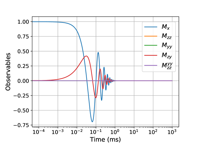
Figure 1: Dynamics of the two-spin observables in the absence of the drive i.e. $\omega_{1}=0$ kilo-rad/s. The time-axis is in log scale. The legends denote $M_{x}(t)$, $M^{\rm yy}_{\rm zz}(t)$, $M_{zz}(t)$, $M_{yy}(t)$ and $M_{zy}(t)$. $\omega_{d}=2\pi\times 5$ kilo-rad/s.

Fig. 1 shows the dynamics of the relevant two-spin variables in the absence of the drive i.e. $\omega_{1}=0$ kilo-rad/s. In this case, after an initial transience, the magnitude of $M_{x}(t)$ becomes vanishingly small in the steady-state, as discussed before. Importantly, values of $M_{zz}(t)$ and $M_{yy}(t)$ remain zero throughout the dynamics as these terms are not created from an initial collective coherence, in the absence of the drive.

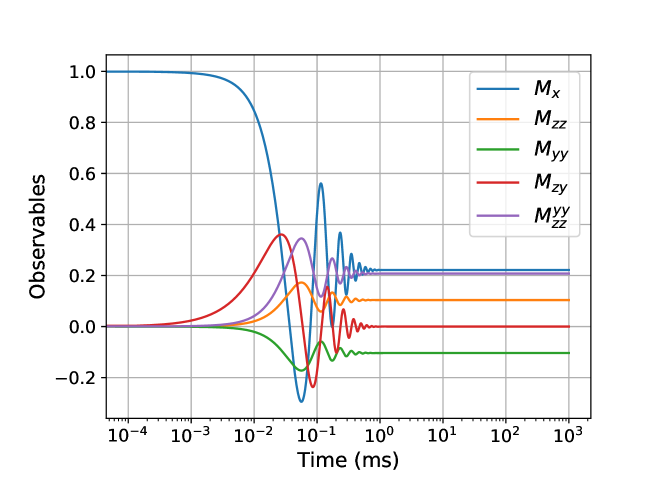
Figure 2: Dynamics of the two-spin observables in the presence of a drive of amplitude $\omega_{1}=2\pi\times 2$ kilo-rad/s. The time-axis is in log scale. The legends denote $M_{x}(t)$, $M^{\rm yy}_{\rm zz}(t)$, $M_{zz}(t)$, $M_{yy}(t)$ and $M_{zy}(t)$. $\omega_{d}=2\pi\times 5$ kilo-rad/s. Initial oscillations indicate rapid inter-conversions between the measured values of the different observables. The non-vanishing steady-state of $M_{x}$ illustrates a persistent collective coherence.

The case in which the drive has a non-zero amplitude of $\omega_{1}=2\pi\times 2$ kilo-rad/s, is shown in Fig. 2. We find that unlike Fig. 1, here we have a non-zero steady-state value of $M_{x}(t)$ after the initial transience, illustrating the emergence of a persistent collective coherence. The steady-state values of $M_{zz}(t)$ and $M_{yy}(t)$ are also non-zero in this case, as expected. A careful inspection of Fig. 2 reveals that the initial $M_{x}$ gets rapidly converted to $M_{yy}$, $M_{zz}$ and $M_{zy}$ in the transient phase. When the variables $M_{yy}$ and $M_{zz}$ have appreciable magnitude, they get re-converted to $M_{x}$ to a large extent, resulting in the oscillatory dynamics illustrated in Fig. 2. Finally, the oscillations die down to result in the steady-state collective coherence.

To study the behavior of the two-spin dynamics for different drive amplitudes, we plot $M_{x}(t)$ from the solutions of Eq. (III.2) for different values of $\omega_{1}$ in Fig. 3. From Fig. 3 it is evident that our equations predict a faster emergence of the quasi-equilibrium state with increasing drive amplitude. Also, the transient oscillations become more prominent with decreasing strength of the drive, as observed in the experiments of Mansfield and Ware manwar68 . In our problem, the damping rate of transients is obtained from equation (12) as $\frac{1}{4}k^{2}\tau_{c}=4\omega_{1}^{2}\tau_{c}+\frac{9}{4}\omega_{d}^{2}\tau_{c}$. Thus higher drive amplitudes induce faster damping of transients (drive-induced-damping), a feature unique to the FRQME approach chakrabarti2018b .

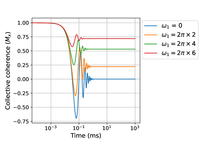
Figure 3: Emergence of the steady-state collective coherence ($M_{x}$) at different values of the drive strength, $\omega_{1}$ in kilo-rad/s. The time-axis is in log scale and $\omega_{d}=2\pi\times 5$ kilo-rad/s.

IV Discussions

Remarkably, the steady-state value of $M_{x}(t)$, given in equation (13), exactly matches the form of the quasi-equilibrium $x$-magnetization, obtained in spin-locking experiments performed on dipolar spin-networks. abragam06 ; manwar68 . In our case, $\frac{9}{4}\omega_{d}^{2}$ plays the role of the squared amplitude of the local field, which appears in the denominator of this quasi-equilibrium expression abragam06 ; manwar68 . We note that no other QME can predict this form of the steady-state magnetization, even though experimental confirmation of this form was obtained in the early days of magnetic resonance spectroscopy manwar68 . It is also important to note that Mansfield and Ware’s fourth-order the perturbative approach is also incapable of predicting this result manwar68 .

We identify the persistent coherence to be the prethermal state as reported in Beatrez and others’ work beatrez21 . If we include the system-environment coupling, we will have $T_{2}$ process which would eventually lead the coherence to zero value, as an unrestrained thermalization process. We note that in the dynamics described by Eq. (III.2) there exists four conserved quantities, which are $M_{yy}+M_{zz}$, $2\omega_{1}M_{x}+3\omega_{d}(M_{yy}-M_{zz})$, $M_{xx}$ and $\text{Tr}\{\rho_{s}\}$. The second of the preceding list ensures the existence of the persistent coherence as long as $\left(2\omega_{1}M_{x}+3\omega_{d}(M_{yy}-M_{zz})\right)|_{t=0}\neq 0.$

The dipolar Hamiltonian (4) transforms as a rank 2 spherical tensor while the drive Hamiltonian is a rank 1 tensor. Cross-relaxations induced by these two Hamiltonians open up the possibility of studying their interplay in the dynamics. Only the FRQME approach can account for these cross-correlations between drive and dipolar Hamiltonians, which lead to the emergence of a prethermal persistent collective coherence. Most importantly, the dynamics predicted by FRQME match with previous experimental observations, which were not addressed by other QME techniques. The unique features of these cross terms (proportional to $\omega_{1}\omega_{d}\tau_{c}$) is that they couple two-spin observables of rank 1, $\sigma_{x}^{(1)}+\sigma_{x}^{(2)}$ to observables of rank 2, $\sigma_{y}^{(1)}\sigma_{y}^{(2)}$ and $\sigma_{z}^{(1)}\sigma_{z}^{(2)}$. We note that these terms modify the rate with which the transients decay and are responsible for giving rise to decay channels for which the the conserved quantities emerge.

V Conclusions

Formulation of the FRQME for a driven, dipolar two-spin ensemble, leads to cross-correlated relaxation between drive and dipolar Hamiltonians, in the second order. We have shown that these cross terms are responsible for the emergence of a prethermal, persistent collective coherence, in suitable limits. Due to the explicit presence of an exponential regulator in all second-order terms of FRQME, arising from the average effect of fluctuations in the local environments, the cross-correlated relaxation terms become independent of the coarse-graining interval. Other time-non-local QME formulations, which do not have an explicit exponential regulator in the second order, can not account for such cross-correlated relaxation effects. Thus, the bath fluctuations play a subtle but very crucial role in the emergence of the prethermal regime.

Particularly, the agreement of our results with previous theoretical and experimental findings indicates that the phenomenon of spin-locking in magnetic resonance can indeed be attributed to the interplay of drive and the dipolar interactions in the second order. Our method also accounts for the drive-dependent damping of transient oscillations observed in the transient phase, which could not be explained by previous approaches. Unlike a typical magnetic resonance experiment performed on a dipolar spin network, our present analysis is only concerned with a dipolar two-spin ensemble. However, the similarity of our results with magnetic resonance experiments indicates the possibility of extending the present analysis to spin-networks via a mean-field approach. On the other hand, the prethermal state of the two-spin ensemble may be used as a short-term storage of quantum correlations. It is simple to implement, requiring a dipolar two-spin ensemble (which can be easily engineered) and a resonant drive. The initial coherence can be created through a simple $\frac{\pi}{2}$ pulse, and the drive should be in phase with this coherence. Also, we envisage that the novel cross-terms in the FRQME may provide deeper insights into the mechanisms of dynamic nuclear polarization (DNP) techniques, which are of considerable theoretical and practical interest folblumahumayac09 ; pedfre72 ; maldebbajhujoomaksirvanhertemgri08 ; puchhoseleskta13 ; thawitkaucor17 .

VI Acknowledgments

Authors gratefully acknowledge insightful discussions and critical comments on the manuscript by Saptarshi Saha and Yeshma Ibrahim.

References

- (1) A. Eckardt, Rev. Mod. Phys. 89,011004, (2017).
- (2) C. Fleckenstein and M. Bukov, Phys. Rev. B 103, L140302, (2021).
- (3) W. Beatrez, O. Janes, A. Akkiraju, A. Pillai, A. Oddo, P. Reshetikhin, E. Druga, M. McAllister, M. Elo, B. Gilbert, D. Suter and A. Ajoy, Phys. Rev. Lett. 127, 170603, (2021).
- (4) L. D’Alessio and M. Rigol, Phys. Rev. X 4, 041048, (2014).
- (5) A. Sen, D. Sen and K. Sengupta, J. Phys.: Condens. Matter 33, 443003, (2021).
- (6) L. F. Santos, Nat.Phys. 17, 429 (2021).
- (7) N. Goldman and J. Dalibard, Phys. Rev. X 4, 031027, (2014).
- (8) M. Bukov, L. D’Alessio and A. Polkovnikov, Adv.Phys. 64, 139, (2015).
- (9) K. Singh, C. J. Fujiwara, Z. A. Geiger, E. Q. Simmons, M. Lipatov, A. Cao, P. Dotti, S. V. Rajagopal, R. Senaratne, T. Shimasaki, M. Heyl, A. Eckardt, and D. M. Weld, Phys. Rev. X 9, 041021, (2019).
- (10) A. Anglés-Castillo, M. C. Bañuls , A. Pérez and I. De Vega, New J. Phys. 22, 083067, (2020).
- (11) I. A. Grigorenko and D. V. Khveshchenko, Phys. Rev. Lett. 94, 040506, (2005).
- (12) Q. V. Lawande, B. N. Jagatap and S. V. Lawande, Phys. Rev. A 42, 4343, (1990).
- (13) C. D. Parmee and N. R. Cooper, Phys. Rev. A 95, 033631, (2017).
- (14) C. D. Parmee and N. R. Cooper, Phys. Rev. A 97, 053616, (2018).
- (15) C. D. Parmee and N. R. Cooper, J. Phys. B: At. Mol. Opt. Phys. 53, 135302, (2020).
- (16) H. Landa, M. Schiró and G. Misguich, Phys. Rev. Lett. 124, 043601, (2020).
- (17) A. Chakrabarti and R. Bhattacharyya, Phys. Rev. A 97, 063837 (2018).
- (18) A. Chakrabarti and R. Bhattacharyya, Europhys. Lett. 121, 57002 (2018).
- (19) A. Chatterjee and R. Bhattacharyya, Phys. Rev. A 102, 043111 (2020).
- (20) N. Chanda and R. Bhattacharyya, Phys. Rev. A 101, 042326 (2020).
- (21) N. Chanda and R. Bhattacharyya, Phys. Rev. A 104, 022436 (2021).
- (22) C. Cohen-Tannoudji, J. Dupont-Roc and G. Gilbert, Atom-Photon Interactions: Basic Processes and Applications WILEY-VCH Verlag GmbH & Co. KGaA, Weinheim, Germany, 2004.
- (23) D. Farfurnik, Y. Horowicz and N. Bar-Gill, Phys. Rev. A 98, 033409, (2018).
- (24) P. Mansfield and D. Ware, Phys. Rev. 168, 318, (1968).
- (25) A. Abragam, The Principles of Nuclear Magnetism Clarendon Press, Oxford, 2006.
- (26) S. Foletti, H. Bluhm, D. Mahalu, V. Umansky and A. Yacoby, Nat. Phys. 5, 903, (2009).
- (27) J. B. Pedersen and J. H. Freed, J. Chem. Phys. 58, 2746, (1972).
- (28) T. Maly, G. T. Debelouchina, V. S. Bajaj, K-N. Hu, C-G. Joo, M. L. Mak–Jurkauskas, J. R. Sirigiri, P. C. A. van der Wel,J. Herzfeld, R. J. Temkin, and R. G. Griffin, J. Chem. Phys. 128, 052211, (2008).
- (29) J. Puebla, E. A. Chekhovich, M. Hopkinson, P. Senellart, A. Lemaitre, M. S. Skolnick, and A. I. Tartakovskii, Phys. Rev. B, 88, 045306, (2013).
- (30) A. S. L. Thankamony, J. J. Wittmann, M. Kaushik and B. Corzilius, Prog. Nucl. Magn. Reson. Spectrosc. 102, 120, (2017).