Optimal Control of Systems with Multichannel Packet Loss

Abstract

The performance of control systems with input packet losses on the controller to plant communication channel is analysed. The main contribution of this work is a proof that linear optimal control systems operating with UDP-like communication protocols have a larger quadratic cost than the same systems operating with TCP-like protocols. The proof is derived for the general case of multidimensional and independent actuation communication channels. In doing so, our results extend previous work to systems with multiple distributed actuators. The difference in cost between two communication protocols is analysed, enabling the maximal difference between the two protocols to be quantified. Numerical examples are presented to highlight the difference in costs induced by the choice of communication protocol.

I Introduction

The surge in number of sensors and smart actuators comes with an increase in wiring within a control system [1]. To this end, wireless communication technology is a readily available tool to reduce the weight and architectural issues of this additional wiring [2, 3, 1]. Wireless control architectures are attractive in a number of applications, such as aerospace, where reductions in the weight and complexity of the cabling between plant and controller offers significant cost savings [3], subject, of course, to safety considerations. Additionally, to be applicable to a control system with multiple actuators the modelling requires a dedicated communication channel for each actuator as opposed to a single communication channel shared by all actuators. However, associated with wireless communication is the issue of packet loss [2, 3]. For communication systems with packet loss, Denial of Service (DoS) attacks are a concern [4]. Moreover, DoS attacks can be implemented within a distributed control system to target individual actuators. A generalisation of a singular communication channel, as seen in [5], is required to analyse the closed-loop performance degradation incurred by packet loss in individual channels.

The multidimensional communication channel considered is an extension of the actuator channel model used in [5] where the channel is modelled as a scalar variable. The main result is the derivation of the optimal control law for a system communicating over multiple independent lossy actuation communication channels, operating under two different communication protocols. This enables the characterisation of the cost difference between the two different communication protocols.

In [5, 6, 7, 8], two communication protocols are proposed for analysis, namely, a TCP-like protocol and a UDP-like protocol. The TCP-like protocol implements an acknowledgement signal that is transmitted back to the controller, confirming whether or not the control signal has been successfully received by the plant. In contrast, the UDP-like protocol lacks the acknowledgement link. The TCP-like protocol differs from the TCP protocol used in communication literature in that a lost packet is not automatically re-transmitted to the plant since there is no reason for this to be useful any longer to the optimal control input. This is due to the most recently calculated control signal being the most vital for the plant to receive. For example, due to the fact that there is no estimation performed at the plant, in addition to the presence of uncertainty within the system, the most recent measurement contains the least uncertainty of the current state of the system. In the event of a packet loss, the plant performs no actuation as is assumed in [5, 6, 7, 8] and is the main focus of [9]. In [5, 9, 7, 8, 6, 10], control systems with packet loss in the communication channels between the plant and the controller are modelled and analysed. In doing so, the foundations for control and estimation over lossy communication channels are established. The optimal control law and estimator is derived for both protocols in [5] using dynamic programming. A control system that is susceptible to packet loss on the communication channel from the plant to the controller is considered in [10]. In [5] and [8] the work of [10] is extended to systems with packet loss in both the sensing (plant to controller channel) and the actuation (controller to plant channel) communication channels. In [9], a comparison of different control strategies in the event of packet loss is studied. They study the effect of a smart actuator that supplies the previous input in the event of a packet loss. Therein they conclude that there exists a trade off between the zero-input and the hold-input strategies. Specifically, in the high packet loss percentage scenario or the ‘cheap control’ scenario the zero-input strategy is superior in terms of Linear Quadratic Gaussian (LQG) cost. Where ‘cheap control’ corresponds to a control law that does not penalise the actuators heavily. Furthermore, the stability regions for both strategies are the same. For that reason, in our work the zero-input strategy is adopted for mathematical simplicity. In [6] and [7], systems with and without an acknowledgement link respectively are considered. These approaches analyse the performance of the controller, and characterise the trade-off between the control system cost, stability, and the properties of the communication channel.

We consider systems that consists of a plant, a controller and a communication channel, as shown in Fig. 1 and 2. This system communicates with one of two communication protocols, a TCP-like protocol or a UDP-like protocol. Packet loss only occurs in the controller to actuator communication channel; the sensor to controller communication channel is assumed to be perfect. This is done to focus on the impact of the actuation channel within a control setting. The analysis in this paper can be extended to the case with a lossy sensor. The actuation communication channel is extended from the previous work [5] to allow for multiple independent channels as opposed to a single channel shared by all actuators. As a result of this, the main contribution is an analytical proof that the system cost is always greater as a result of not monitoring realisations of packet loss in the channel. The maximal cost difference between the two protocols is also characterised. The packet loss in the communication channel is modelled as a set of Independent and Identically Distributed (IID) Bernoulli random variables. As a result, each actuator either receives the optimal input, or it receives zero input. This is equivalent to a probabilistic Denial of Service attack on the communication channel. The optimal control law is obtained by formulating the problem in a Model Predictive Control (MPC) framework. This subsequently enables the analytical comparison of the cost incurred by both protocols in a more tractable fashion that a dynamic programming approach.

The structure of the rest of the paper is as follows, Section II describes the system model and the MPC framework; Section III contains the main results and the derivation of the optimal control law for both protocols; Section IV characterises the cost difference between the protocols; Section V contains numerical results from two illustrative case studies; Section VI discusses the implications of utilising a multidimensional channel, based upon the second case study; and Section VII presents the conclusion.

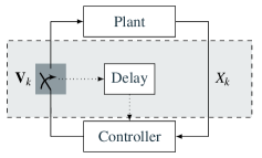
Figure 1: The TCP-like protocol where realisations of the packet transmission variable, ${\bf V}_{k}$, are transmitted to the controller.

II System Model and Problem Formulation

We consider the plant model described by

$$X_{k\scalebox{0.5}[0.5]{$+$}1} = {\bf A}X_{k}+{\bf B}{{\bf V}_{k}}U_{k}+W_{k},$$ (1)

where ${\bf A}\in\mathds{R}^{n\times n}$ is the dynamics matrix; $X_{k}\in\mathds{R}^{n}$ describes the state of the plant at time step $k\in\mathds{N}$; ${\bf B}\in\mathds{R}^{n\times m}$ is the control matrix; ${U}_{k}\in\mathds{R}^{m}$ is the vector of control inputs; $W_{k}\in\mathds{R}^{n}$ is the process noise modelled as a vector of Gaussian random variables with mean ${\bf 0}\in\mathds{R}^{n}$ and covariance matrix $\Sigma_{W}\in S^{n}_{++}$; where $S^{n}_{++}$ is the set of $n$ by $n$ symmetric positive definite matrices; ${\bf V}_{k}\in S^{m}_{+}$ is the packet transmission variable modelled as a diagonal matrix where the $i$-th diagonal entry is an IID Bernoulli random variable with mean $\mu_{i}\in\left[0,1\right]$; and $S^{m}_{+}$ is the set of $m$ by $m$ symmetric non-negative definite matrices. The initial state of the plant is determined by the Gaussian distributed vector of random variables $X_{k}$ with mean ${\overline{X}_{k}}$ and covariance matrix  ${\Sigma_{X_{k}}}\in S^{n}_{++}$. Additionally, the expected value of ${\bf V}_{k}$ is $\mbox{\bb E}[{\bf V}_{k}]={\bf M}$, where ${\bf M}\in S^{m}_{++}$ is a diagonal matrix in which the i-th diagonal element is $\mu_{i}$.

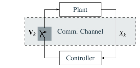
Figure 2: The UDP-like protocol where the realisations of the packet transmission variable, ${\bf V}_{k}$, are not transmitted to the controller

It is in the structure of ${\bf V}_{k}$ and ${\bf M}$ that the system model differs from [5, 9, 7, 8, 6, 10]. Defining ${\bf M}$ as a matrix models the case in which the system communicates over $m$ independent channels, where each actuator has a single dedicated communication channel. Specifically, the $m$-th control input communicates through the $m$-th channel which is completely characterised by the $m$-th diagonal entry of ${\bf M}$. In contrast, were ${\bf M}$ and ${\bf V}_{k}$ to be defined as a scalars all control inputs would share a single communication channel that is fully characterised by these scalars. This setting generalises the packet loss communication channel seen in [5]. Due to the imperfect communication between the controller and the plant, the operator implements a communication protocol. We adopt two protocol paradigms proposed by [5], namely a UDP-like protocol that does not monitor the communication channel, and a TCP-like protocol that acknowledges receipt of the packet from the controller by sending an acknowledgement message to the controller over an auxiliary channel. As in [5] it is assumed that the auxiliary channel has perfect communication. The difference between both protocol paradigms is depicted in Fig. 1 and Fig. 2 for the TCP-like and the UDP-like protocols respectively. The choice of protocol paradigm for a system results in different information available for the controller. We define the information available at the controller for each protocol with the following two information sets

$${\cal I}_{k}\stackrel{{\scriptstyle\Delta}}{{=}}\begin{cases}{\cal F}_{k}=\left\{{\cal X}^{k},{\cal V}^{k\scalebox{0.5}[1.0]{$-$}1}\right\},&\mbox{TCP-like},\\ {\cal G}_{k}=\left\{{\cal X}^{k}\right\},&\mbox{UDP-like},\\ \end{cases}$$ (2)

where ${\cal V}^{k\scalebox{0.5}[1.0]{$-$}1}\stackrel{{\scriptstyle\Delta}}{{=}}\left\{{\bf V}_{0},{\bf V}_{1},\ldots,{\bf V}_{k\scalebox{0.5}[1.0]{$-$}1}\right\}$ and ${\cal X}^{k}\stackrel{{\scriptstyle\Delta}}{{=}}\left\{X_{0},X_{1},\dots,X_{k}\right\}$. Note that all sets are monotonically increasing, i.e. ${\cal I}_{k}\subseteq{\cal I}_{k\scalebox{0.5}[0.5]{$+$}1}$. Additionally, the lower indices represent the time index whereas upper indices refers to the dimension. The information set at each time step contains the information from all previous time steps in addition to the information from the current time step. Under the TCP-like protocol the controller has access to the realisation of the packet transmission variable, ${\bf V}_{k}$, when performing state estimation and incorporates it in the error prediction to obtain an estimate with error

$$E_{k\scalebox{0.5}[0.5]{$+$}1}\!\left(\!{\cal F}_{k}\!\right)\mkern-18.0mu\ \stackrel{{\scriptstyle\Delta}}{{=}} \mkern-18.0mu\ X_{k\scalebox{0.5}[0.5]{$+$}1}-\mbox{\bb E}\left[X_{k\scalebox{0.5}[0.5]{$+$}1}{\Big{|}}{\cal F}_{k},{\bf V}_{k}\right]$$ (3a)

$$= \mkern-18.0mu\ {\bf A}X_{k}+{\bf B}{{\bf V}_{k}}U_{k}\!\left(\!{\cal F}_{k}\!\right)+W_{k}-{\bf A}\widehat{X}_{k}-{\bf B}{{\bf V}_{k}}U_{k}\!\left(\!{\cal F}_{k}\!\right)$$

$$= \mkern-18.0mu\ {\bf A}E_{k}\!\!\left(\!{\cal F}_{k\scalebox{0.5}[1.0]{$-$}1}\!\right)\!\!+W_{k},$$

where $$\widehat{X}_{k}\stackrel{{\scriptstyle\Delta}}{{=}}\mbox{\bb E}\left[X_{k}\right] U_{k}\!\left(\!{\cal I}_{k}\!\right) {\cal I}_{k} {\bf V}_{k}$$. The function  is a function of the information set  and takes the form of a state feedback law, and is therefore, a random variable,. The UDP-like protocol error prediction differs from the TCP-like protocol in that there is no knowledge of the realisation of , and therefore, the error for the UDP-like protocol is given by

$$E_{k\scalebox{0.5}[0.5]{$+$}1}\!\left(\!{\cal G}_{k}\!\right)\mkern-18.0mu\ \stackrel{{\scriptstyle\Delta}}{{=}} \mkern-18.0mu\ X_{k\scalebox{0.5}[0.5]{$+$}1}-\mbox{\bb E}\left[X_{k\scalebox{0.5}[0.5]{$+$}1}{\Big{|}}{\cal G}_{k}\right]$$ (3b)

$$= \mkern-18.0mu\ {\bf A}X_{k}+{\bf B}{{\bf V}_{k}}U_{k}\!\left(\!{\cal G}_{k}\!\right)+W_{k}-{\bf A}\widehat{X}_{k}-{\bf B}{\bf M}U_{k}\!\left(\!{\cal G}_{k}\!\right)$$

$$= \mkern-18.0mu\ {\bf A}E_{k}\!\!\left(\!{\cal G}_{k\scalebox{0.5}[1.0]{$-$}1}\!\right)\!\!+{\bf B}\left({\bf V}_{k}-{\bf M}\right)U_{k}\!\left(\!{\cal G}_{k}\!\right)+W_{k}.$$

Note that the error prediction for both the UDP-like and the TCP-like protocol resemble those in [5]. As shown in [5], the optimal linear control law for the UDP-like protocol can only be obtained when perfect state information is available. Indeed, the lack of knowledge about the packet loss breaks the separation structure between optimal estimation and optimal control. It is here our derivation diverges again from [5]. Assuming perfect knowledge of the realisation of $X_{k}$, (1) is expanded over a time horizon $N\in\mathds{N}$ as follows:

$$\!\!\!\!\begin{array}[]{c}X_{k\scalebox{0.5}[0.5]{$+$}1}\\ X_{k\scalebox{0.5}[0.5]{$+$}2}\\ \vdots\\ X_{k\scalebox{0.5}[0.5]{$+$}N}\end{array}\!\!\!\!\!\!\!\!\begin{array}[]{c}=\\ =\\ {\vdots}\\ =\end{array}\mkern-18.0mu\begin{array}[]{c}{\bf A}X_{k}\\ {\bf A}X_{k\scalebox{0.5}[0.5]{$+$}1}\\ \vdots\\ {\bf A}X_{k\scalebox{0.5}[0.5]{$+$}N\scalebox{0.5}[1.0]{$-$}1}\end{array}\mkern-18.0mu\begin{array}[]{c}+\\ +\\ \vphantom{\vdots}\\ +\end{array}\mkern-18.0mu\begin{array}[]{c}{\bf B}{\bf V}_{k}U_{k}\!\left(\!{\cal I}_{k}\!\right)\\ {\bf B}{\bf V}_{k\scalebox{0.5}[0.5]{$+$}1}U_{k\scalebox{0.5}[0.5]{$+$}1}\!\left(\!{\cal I}_{k}\!\right)\\ \vdots\\ {\bf B}{\bf V}_{k\scalebox{0.5}[0.5]{$+$}N\scalebox{0.5}[1.0]{$-$}1}U_{k\scalebox{0.5}[0.5]{$+$}N\scalebox{0.5}[1.0]{$-$}1}\!\left(\!{\cal I}_{k}\!\right)\end{array}\mkern-18.0mu\begin{array}[]{c}+\\ +\\ \vphantom{\vdots}\\ +\end{array}\mkern-18.0mu\begin{array}[]{c}W_{k},\\ W_{k\scalebox{0.5}[0.5]{$+$}1},\\ \vdots\\ W_{k\scalebox{0.5}[0.5]{$+$}N\scalebox{0.5}[1.0]{$-$}1}.\end{array}\!\!\!\!\!\!$$ (32)

Exploiting the recursive structure yields

$$X_{k\scalebox{0.5}[0.5]{$+$}1}\mkern-18.0mu = \mkern-18.0mu{\bf A}X_{k}+{\bf B}{\bf V}_{k}U_{k}\!\left(\!{\cal I}_{k}\!\right)+W_{k},$$

$$X_{k\scalebox{0.5}[0.5]{$+$}2}\mkern-18.0mu = \mkern-18.0mu{\bf A}^{2}X_{k}+{\bf A}{\bf B}{\bf V}_{k}U_{k}\!\!\left(\!{\cal I}_{k}\!\right)+{\bf B}{\bf V}_{k\scalebox{0.5}[0.5]{$+$}1}U_{k\scalebox{0.5}[0.5]{$+$}1}\!\!\left(\!{\cal I}_{k}\!\right)+{\bf A}W_{k}+W_{k\scalebox{0.5}[0.5]{$+$}1},$$

$$\vdots$$

$$X_{k\scalebox{0.5}[0.5]{$+$}N}\mkern-18.0mu = \mkern-18.0mu{\bf A}^{N}X_{k}\!+\!{\bf A}^{N\scalebox{0.5}[1.0]{$-$}1}{\bf B}{\bf V}_{k}U_{k}\!\left(\!{\cal I}_{k}\!\right)\!+\!\dots$$

$$\mkern-18.0mu+{\bf B}{\bf V}_{k\scalebox{0.5}[0.5]{$+$}N\scalebox{0.5}[1.0]{$-$}1}U_{k\scalebox{0.5}[0.5]{$+$}N\scalebox{0.5}[1.0]{$-$}1}\!\left(\!{\cal I}_{k}\!\right)+{\bf A}^{N\scalebox{0.5}[1.0]{$-$}1}W_{k}+\dots+W_{k\scalebox{0.5}[0.5]{$+$}N\scalebox{0.5}[1.0]{$-$}1}.$$

$$\!\!\!\!\underset{\pazocal{X}_{k}}{\underbrace{\left(\!\!\!\!\begin{array}[]{c}X_{k\scalebox{0.5}[0.5]{$+$}1}\\ X_{k\scalebox{0.5}[0.5]{$+$}2}\\ \vdots\\ X_{k\scalebox{0.5}[0.5]{$+$}N}\end{array}\!\!\!\!\right)}}\!\!\!=\!\!\!\underset{\Phi}{\underbrace{\left(\!\!\!\!\begin{array}[]{c}{\bf A}\\ {\bf A}^{2}\\ \vdots\\ {\bf A}^{N}\end{array}\!\!\!\!\right)}}\!X_{k}\!+\!\!\!\underset{\Gamma}{\underbrace{\left(\!\!\!\!\begin{array}[]{cccc}{\bf B}&\bf 0&\dots&\bf 0\\ {\bf A}{\bf B}&{\bf B}&\ddots&\vdots\\ \vdots&\ddots&\ddots&\bf 0\\ {\bf A}^{N\scalebox{0.5}[1.0]{$-$}1}{\bf B}&\dots&{\bf A}{\bf B}&{\bf B}\end{array}\!\!\!\!\right)}}\ \underset{\ \!\!\Upsilon_{k}\!\!\ }{\underbrace{\left(\!\!\!\!\!\!\begin{array}[]{cccc}{\bf V}_{k}&\bf 0&\dots&\bf 0\\ \bf 0&{\bf V}_{k\scalebox{0.5}[0.5]{$+$}1}&\ddots&\vdots\\ \vdots&\ddots&\ddots&\bf 0\\ \bf 0&\dots&\bf 0&{\bf V}_{k\scalebox{0.5}[0.5]{$+$}N\scalebox{0.5}[1.0]{$-$}1}\end{array}\!\!\!\!\!\!\right)}}\!\!\underset{\pazocal{U}_{k}\!\left(\!{\cal I}_{k}\!\right)}{\underbrace{\left(\!\!\!\!\!\!\begin{array}[]{c}U_{k}\!\!\left(\!{\cal I}_{k}\!\right)\\ U_{k\scalebox{0.5}[0.5]{$+$}1}\!\!\left(\!{\cal I}_{k}\!\right)\\ \vdots\\ U_{k\scalebox{0.5}[0.5]{$+$}N\scalebox{0.5}[1.0]{$-$}1}\!\!\left(\!{\cal I}_{k}\!\right)\end{array}\!\!\!\!\!\!\right)}}\!\!+\!\!\underset{\Lambda}{\underbrace{\left(\!\!\!\!\!\!\begin{array}[]{cccc}{\bf I}&\bf 0&\dots&\bf 0\\ {\bf A}&{\bf I}&\ddots&\vdots\\ \vdots&\ddots&\ddots&\bf 0\\ {\bf A}^{N\scalebox{0.5}[1.0]{$-$}1}&\dots&{\bf A}&{\bf I}\end{array}\!\!\!\!\right)}}\!\underset{\pazocal{W}_{k}}{\underbrace{\left(\!\!\!\!\!\!\begin{array}[]{c}W_{k}\\ W_{k\scalebox{0.5}[0.5]{$+$}1}\\ \vdots\\ W_{k\scalebox{0.5}[0.5]{$+$}N\scalebox{0.5}[1.0]{$-$}1}\end{array}\!\!\!\!\!\!\right)}}$$ (61)

Re-writing (II) in matrix form yields (61) seen at the top of the next page. Re-casting (61) as a prediction matrix equation gives

$${\pazocal{X}}_{k}\stackrel{{\scriptstyle\Delta}}{{=}}\Phi X_{k}+\Gamma{\ \!\!\Upsilon_{k}\!\!\ }\pazocal{U}_{k}\!\left(\!{\cal I}_{k}\!\right)+\Lambda{\pazocal{W}}_{k},$$ (62)

where $\Phi\in\mathds{R}^{Nn\times n}$ is the dynamics matrix over the prediction horizon; $\pazocal{X}_{k}\in\mathds{R}^{Nn}$ is the state prediction vector; $\Gamma\in\mathds{R}^{Nn\times Nm}$ is the propagation matrix for the control over the prediction horizon; ${\pazocal{U}_{k}}\!\!\left(\!{\cal I}_{k}\!\right)\!\!\in\mathds{R}^{Nm}$ is the realisation at time step $k$ of the control law computed with access to the information set ${\cal I}_{k}$; $\Lambda\in\mathds{R}^{Nn\times Nn}$ is the propagation matrix for the process noise; ${\pazocal{W}_{k}}\in\mathds{R}^{Nn}$ is the process noise over the prediction horizon with mean $\bf 0$ and covariance $\Sigma_{\pazocal{W}}$; $\Sigma_{\pazocal{W}}\in S^{Nn}_{++}$ is the diagonal block matrix where the $i$-th block is $\Sigma_{W}$;  $\ \!\!\Upsilon_{k}\!\!\ \in S^{Nm}_{+}$ is a diagonal matrix with the Bernoulli random variables describing the packet transmission over the prediction horizon in the diagonal;and $\ \!\!\overline{\Upsilon}\!\!\ \in S^{Nm}_{++}$ is the block diagonal matrix where the $i$-th block is ${\bf M}$, and therefore, $\mbox{\bb E}\left[\ \!\!\Upsilon_{k}\!\!\ \right]=\ \!\!\overline{\Upsilon}\!\!\$. To control the system over the horizon, N, the controller calculates the expected state trajectory, $\widehat{\pazocal{X}}_{k}$. Note that for both protocols the estimate coincides, due to the fact that neither protocol knows the realisation of ${\bf V}_{k}$ before actuating. The expected state trajectory for both protocols is therefore given by

$$\widehat{\pazocal{X}}_{k}\stackrel{{\scriptstyle\Delta}}{{=}}\mbox{\bb E}\left[{\pazocal{X}}_{k}{\Big{|}}{\cal I}_{k}\right]=\Phi X_{k}+\Gamma\ \!\!\overline{\Upsilon}\!\!\ {\pazocal{U}_{k}\!\left(\!{\cal I}_{k}\!\right)}.$$ (63)

In the TCP-like regime the operator does not know the realisation of a packet transmission before actuating, which results in (63), but knows the packet transmission realisation when updating the state estimate, which results in (3a). The TCP-like protocol only estimates the packet transmission for the optimal control problem. In contrast, the UDP-like protocol packet transmission variables are estimated for both the estimation and the optimal control problem. Expanding the update error terms in (3) over the prediction horizon of $N$ time-steps results in

$${\bf E}_{k}\!\left(\!{\cal F}_{k}\!\right)\mkern-18.0mu\ \stackrel{{\scriptstyle\Delta}}{{=}} \mkern-18.0mu\ {\pazocal{X}}_{k}-\mbox{\bb E}\left[{\pazocal{X}}_{k}{\Big{|}}{\cal F}_{k},\ \!\!\Upsilon_{k}\!\!\ \right]$$ (64a)

$$= \mkern-18.0mu\ \Phi X_{k}+\Gamma{\ \!\!\Upsilon_{k}\!\!\ }{\pazocal{U}_{k}\!\left(\!{\cal F}_{k}\!\right)}+\Lambda{\pazocal{W}}_{k}-\widehat{\pazocal{X}}_{k}$$

$$= \mkern-18.0mu\ \Phi X_{k}+\Gamma{\ \!\!\Upsilon_{k}\!\!\ }{\pazocal{U}_{k}\!\left(\!{\cal F}_{k}\!\right)}+\Lambda{\pazocal{W}}_{k}-\Phi X_{k}-\Gamma{\ \!\!\Upsilon_{k}\!\!\ }{\pazocal{U}_{k}\!\left(\!{\cal F}_{k}\!\right)}$$

$$= \mkern-18.0mu\ \Lambda{\pazocal{W}}_{k},$$

$${\bf E}_{k}\!\left(\!{\cal G}_{k}\!\right)\mkern-18.0mu\ \stackrel{{\scriptstyle\Delta}}{{=}} \mkern-18.0mu\ {\pazocal{X}}_{k}-\mbox{\bb E}\left[{\pazocal{X}}_{k}{\Big{|}}{\cal G}_{k}\right]$$ (64b)

$$= \mkern-18.0mu\ \Phi X_{k}+\Gamma{\ \!\!\Upsilon_{k}\!\!\ }{\pazocal{U}_{k}\!\left(\!{\cal F}_{k}\!\right)}+\Lambda{\pazocal{W}}_{k}-\widehat{\pazocal{X}}_{k}$$

$$= \mkern-18.0mu\ \Phi X_{k}+\Gamma{\ \!\!\Upsilon_{k}\!\!\ }{\pazocal{U}_{k}\!\left(\!{\cal G}_{k}\!\right)}+\Lambda{\pazocal{W}}_{k}-\Phi X_{k}-\Gamma\ \!\!\overline{\Upsilon}\!\!\ {\pazocal{U}_{k}\!\left(\!{\cal G}_{k}\!\right)}$$

$$= \Gamma\left(\ \!\!\Upsilon_{k}\!\!\ -\ \!\!\overline{\Upsilon}\!\!\ \right){\pazocal{U}_{k}\!\left(\!{\cal G}_{k}\!\right)}+\Lambda{\pazocal{W}}_{k}.$$

In this setting we formulate a Linear Quadratic Gaussian (LQG) control problem, i.e. the system operator minimises a quadratic function of the states and inputs. This function is weighted with diagonal state penalty matrix $\Omega\in S_{++}^{Nn}$, diagonal input penalty matrix $\Psi\in S_{++}^{Nm}$, and diagonal matrix ${\bf Q}\in S^{n}_{++}$. Note that the penalties at each time step may vary. Since $\pazocal{W}_{k}$ is random, then the state of the plant is random, which yields a stochastic model predictive control problem [11]. The cost function to be minimised is the expected cost defined as

$$J\left(\!{\cal I}_{k}\!\right)\mkern-18.0mu\ \stackrel{{\scriptstyle\Delta}}{{=}} \mkern-18.0mu\ \mbox{\bb E}\left[\left.X_{k}^{\sf T}{\bf Q}X_{k}+{\pazocal{X}}_{k}^{\sf T}\Omega{\pazocal{X}}_{k}\right.\right.$$ (65a)

$$\qquad\qquad\left.\left.+\pazocal{U}^{\sf T}_{k}\!\!\left(\!{\cal I}_{k}\!\right)\!\!\ \!\!\Upsilon_{k}\!\!\ ^{\!\!\!\!\sf T}\Psi\ \!\!\Upsilon_{k}\!\!\ {\pazocal{U}_{k}}\!\!\left(\!{\cal I}_{k}\!\right)\!\right|{\cal I}_{k}\right]\!\!,\!\!$$

where the expectation in (65a) is with respect to the joint distribution of $$\ \!\!\Upsilon_{k}\!\!\ {\pazocal{W}}_{k} 1 X_{k}\rightarrow X_{k\scalebox{0.5}[0.5]{$+$}1}\rightarrow\dots\rightarrow X_{k\scalebox{0.5}[0.5]{$+$}N} {\pazocal{X}}_{k} \widehat{\pazocal{X}}_{k}~{} {\bf E}_{k} \pazocal{X}_{k}=\widehat{\pazocal{X}}_{k}+{\bf E}_{k}$$ and . The expectation is taken sequentially as in [6, Lemma (c)] to account for the causality constraints imposed by the system. Therein, the expectation at each time step is conditioned on all previous time steps. This is due to the fact that the sequence of states at each time step forms a Markov chain, i.e. . The state trajectory  is re-written in terms of the estimate  and the error induced by the estimate . Substituting  into (65a) yields

$$\!\!J\!\!\left(\!{\cal I}_{k}\!\right)\mkern-18.0mu\ = \mkern-18.0mu\ \mbox{\bb E}\!\!\left[\left.\!X_{k}^{\sf T}\!\!{\bf Q}X_{k}\!+\!\left(\widehat{\pazocal{X}}_{k}\!\!+\!{{\bf E}_{k}}\right)^{\sf\!\!T}\!\!\!\Omega\!\left(\widehat{\pazocal{X}}_{k}\!\!+\!{{\bf E}_{k}}\right)\!\right.\right.$$ (65b)

$$\qquad\qquad\left.\left.\vphantom{\left(\widehat{\pazocal{X}}_{k}\!\!+\!{{\bf E}_{k}}\right)^{\sf\!\!T}}+\!{\pazocal{U}_{k}}^{\sf\!\!\!T}\!\!\left(\!{\cal I}_{k}\!\right)\!\!\ \!\!\Upsilon_{k}\!\!\ ^{\sf\!\!T}\!\Psi\ \!\!\Upsilon_{k}\!\!\ {\pazocal{U}_{k}}\!\!\left(\!{\cal I}_{k}\!\right)\!\right|\!{\cal I}_{k}\!\!\right]\!\!.$$

The optimal control problem is to find the input sequence $\pazocal{U}^{*}_{k}$ that minimises (65b). Additionally, it should be noted that $\mbox{\bb E}\left[{\bf E}_{k}{\big{|}}{\cal I}_{k}\right]=0$ and the state error and the state estimate are independent for both protocols. The proofs of these statements are provided in [6]. which leads to the following optimal cost definition:

$$\mkern-36.0muJ^{*}\left(\!{\cal I}_{k}\!\right)\stackrel{{\scriptstyle\Delta}}{{=}}\min_{{\pazocal{U}_{k}}\!\!\left(\!{\cal I}_{k}\!\right)\!}\left\{\mbox{\bb E}\left[X_{k}^{\sf T}{\bf Q}X_{k}+\widehat{\pazocal{X}}_{k}^{\sf T}\Omega\widehat{\pazocal{X}}_{k}+{\bf E}_{k}^{\sf T}\Omega{{\bf E}_{k}}\vphantom{\Big{|}}\right.\right.$$

$$\qquad\qquad\quad\left.\left.\vphantom{\left(\widehat{\pazocal{X}}_{k}\!\!+\!{{\bf E}_{k}}\right)^{\sf\!\!T}}+\!{\pazocal{U}_{k}}^{\sf\!\!\!T}\!\!\left(\!{\cal I}_{k}\!\right)\!\!\ \!\!\Upsilon_{k}\!\!\ ^{\sf\!\!T}\!\Psi\ \!\!\Upsilon_{k}\!\!\ {\pazocal{U}_{k}}\!\!\left(\!{\cal I}_{k}\!\right)\!\right|\!{\cal I}_{k}\!\!\right]\!\!.$$ (66)

III MPC Optimal Cost Derivation and Analysis

The derivation of the optimal control law is therefore recast into solving the minimisation in (II) for both communication protocols. The first and second term on the right hand side of (II) are not random due to the information available and are therefore unaffected by the expectation. Furthermore, since the first term does not depend on ${\pazocal{U}_{k}}$ the minimisation is rewritten as

$$J^{*}\left(\!{\cal I}_{k}\!\right)\!\!\!\!\!\!\!\! = \!\!\!\!\!\!\!\!X_{k}^{\sf T}{\bf Q}X_{k}+\min_{{\pazocal{U}_{k}}\!\!\left(\!{\cal I}_{k}\!\right)\!}\left\{\widehat{\pazocal{X}}^{\sf T}_{k}\Omega\widehat{\pazocal{X}}_{k}\right.$$ (67)

$$\left.\!\!+\mbox{\bb E}\left[\!\!\left.\vphantom{\widehat{\pazocal{X}}^{\sf T}_{k}}{\bf E}_{k}^{\sf T}\Omega{{\bf E}_{k}}+\!{\pazocal{U}_{k}}^{\sf\!\!\!T}\!\!\left(\!{\cal I}_{k}\!\right)\!\!\ \!\!\Upsilon_{k}\!\!\ ^{\sf\!\!T}\!\Psi\ \!\!\Upsilon_{k}\!\!\ {\pazocal{U}_{k}}\!\!\left(\!{\cal I}_{k}\!\right)\!\right|{\cal I}_{k}\right]\right\}\!\!.\quad\$$

The computation of the expectation of the last term can be simplified by using the commutation properties of diagonal matrices and the idempotency of the matrix $\ \!\!\Upsilon_{k}\!\!\$. Additionally, due to the causality imposed on the system, ${\pazocal{U}_{k}}\!\!\left(\!{\cal I}_{k}\!\right)\!$ does not depend on the future realisations of ${\bf V}_{k}$ or $W_{k}$, and therefore, is not affected by the expectation. Note, that this still allows for a ${\pazocal{U}_{k}}\!\!\left(\!{\cal I}_{k}\!\right)\!$ that depends on the statistics of each of these variables, just not the future realisations. The last term in (67) is

$$\mbox{\bb E}\left[\left.\!{\pazocal{U}_{k}}^{\sf\!\!\!T}\!\!\left(\!{\cal I}_{k}\!\right)\!\!\ \!\!\Upsilon_{k}\!\!\ ^{\sf\!\!T}\!\Psi\ \!\!\Upsilon_{k}\!\!\ {\pazocal{U}_{k}}\!\!\left(\!{\cal I}_{k}\!\right)\!\right|{\cal I}_{k}\right]\mkern-18.0mu\ = \mkern-18.0mu\ {\pazocal{U}_{k}\!\left(\!{\cal I}_{k}\!\right)^{\!\!\sf T}}\ \!\!\overline{\Upsilon}\!\!\ \Psi{\pazocal{U}_{k}\!\left(\!{\cal I}_{k}\!\right)}.\ \ \$$ (68)

Therefore, (67) is equivalent to

$$\mkern-36.0muJ^{*}\left(\!{\cal I}_{k}\!\right)=X_{k}^{\sf T}{\bf Q}X_{k}+\min_{{\pazocal{U}_{k}}\!\!\left(\!{\cal I}_{k}\!\right)\!}\left\{\widehat{\pazocal{X}}_{k}^{\sf T}\Omega\widehat{\pazocal{X}}_{k}+{{\pazocal{U}_{k}\!\left(\!{\cal I}_{k}\!\right)}{{}^{\sf T}}}\ \!\!\overline{\Upsilon}\!\!\ \Psi{\pazocal{U}_{k}\!\left(\!{\cal I}_{k}\!\right)}\vphantom{\Big{|}}\right.$$

$$\qquad\qquad\qquad\qquad\qquad\left.+\mbox{\bb E}\left[{\bf E}_{k}^{\sf T}\Omega{{\bf E}_{k}}{\Big{|}}{\cal I}_{k}\right]\right\}.$$ (69)

The term involving the expected state trajectory is combined with (63) to give

$$J^{*}\left(\!{\cal I}_{k}\!\right)\mkern-18.0mu\ = \mkern-18.0mu\ X_{k}^{\sf T}\left({\bf Q}+\Omega_{p}\right)X_{k}+\min_{{\pazocal{U}_{k}}\!\!\left(\!{\cal I}_{k}\!\right)\!}\left\{\mbox{\bb E}\left[{\bf E}_{k}^{\sf T}\Omega{{\bf E}_{k}}{\Big{|}}{\cal I}_{k}\right]\right.$$ (70)

$$\mkern-18.0mu\left.+{\pazocal{U}_{k}\!\left(\!{\cal I}_{k}\!\right)^{\!\!\sf T}}\ \!\!\overline{\Upsilon}\!\!\ \left(2\Omega_{gp}X_{k}+\left(\Omega_{g}\ \!\!\overline{\Upsilon}\!\!\ +\Psi\right){\pazocal{U}_{k}\!\left(\!{\cal I}_{k}\!\right)}\right)\!\!\right\}\!\!,\ \ \$$

where $\Omega_{p}=\Phi^{\sf T}\Omega\Phi$, $\Omega_{g}=\Gamma^{\sf T}\Omega\Gamma$, and $\Omega_{gp}=\Gamma^{\sf T}\Omega\Phi$.

Evaluating the quadratic error requires knowledge of second order statistics. It is in this step that the differences between the UDP-like protocol and the TCP-like protocol become apparent. This observation leads to the first lemma.

Lemma 1

Consider the system modelled by (1) with access to (2). Then the following holds

$$\!\!\mbox{\bb E}\!\!\left[\!{\bf E}_{k}^{\sf T}\!\Omega{{\bf E}_{k}}{\Big{|}}{\cal F}_{k}\right]\mkern-18.0mu\! = \mkern-18.0mu\textnormal{tr}\left(\!\Omega_{l}\Sigma_{\pazocal{W}}\!\right)\!\!,$$ (71a)

$$\!\!\mbox{\bb E}\!\!\left[{\bf E}_{k}^{\sf T}\Omega{{\bf E}_{k}}{\Big{|}}{\cal G}_{k}\right]\mkern-18.0mu = \mkern-18.0mu{\pazocal{U}_{k}\!\left(\!{\cal G}_{k}\!\right)^{\!\!\sf T}}\!\ \!\!\overline{\Upsilon}\!\!\ \!\left({\bf I}\odot\Omega_{g}\right)\!\left({\bf I}-\ \!\!\overline{\Upsilon}\!\!\ \right)\!\!{\pazocal{U}_{k}\!\left(\!{\cal G}_{k}\!\right)}\!$$ (71b)

$$\qquad\qquad+\!\textnormal{tr}\left(\!\Omega_{l}\Sigma_{\pazocal{W}}\!\right)\!\!,\ \quad$$

where $\Omega_{l}=\Lambda\Omega\Lambda$ and $\odot$ denotes the Hadamard product.

Proof:

See Appendix.

Lemma 1 highlights that the UDP-like quadratic error term depends on $\pazocal{U}_{k}\!\left(\!{\cal G}_{k}\!\right)$, whereas the TCP-like protocol does not. Additionally, (70) shows that the quadratic error term lies within the minimisation. Therefore, the term for the TCP-like quadratic error is removed from the minimisation in (70) whereas the UDP-like term is not. Due to this, the derivation of the optimal control law is at this point split into two cases.

Theorem 1

Consider the closed-loop systems shown in Fig. 1 and Fig. 2, with plant dynamics given in (1), protocol dependent information sets given in (2), and controller cost function given in (II), respectively. Then the optimal cost for the TCP-like protocol is

$$J^{*}\left(\!{\cal F}_{k}\!\right)\mkern-18.0mu\ = \mkern-18.0mu\ \!\!X_{k}^{\sf T}\!\!\left({\bf Q}+\Omega_{p}\right)\!\!X_{k}\!+\!\textnormal{tr}\left(\Sigma_{\pazocal{W}}\Omega_{l}\!\right)\!\!$$ (72a)

$$\qquad\qquad-\!X_{k}^{\sf T}\!\Omega_{gp}^{\sf T}\!{\bf G}^{\scalebox{0.5}[1.0]{$-$}1}\!\!\left(\!{\cal F}_{k}\!\right)\!\ \!\!\overline{\Upsilon}\!\!\ \Omega_{gp}X_{k},$$

and the optimal cost for the UDP-like protocol is

$$J^{*}\left(\!{\cal G}_{k}\!\right)\mkern-18.0mu\ = \mkern-18.0mu\ \!\!X_{k}^{\sf T}\!\!\left({\bf Q}+\Omega_{p}\right)\!\!X_{k}\!+\!\textnormal{tr}\left(\Sigma_{\pazocal{W}}\Omega_{l}\!\right)\!\!$$ (72b)

$$\qquad\qquad-\!X_{k}^{\sf T}\!\Omega_{gp}^{\sf T}\!{\bf G}^{\scalebox{0.5}[1.0]{$-$}1}\!\!\left(\!{\cal G}_{k}\!\right)\!\ \!\!\overline{\Upsilon}\!\!\ \Omega_{gp}X_{k}.$$

The corresponding optimal control laws are

$${\pazocal{U}^{{}^{*}}_{k}\!\left(\!{\cal F}_{k}\!\right)}\mkern-18.0mu\ \stackrel{{\scriptstyle\Delta}}{{=}} \mkern-18.0mu\ -\left(\Omega_{g}\ \!\!\overline{\Upsilon}\!\!\ +\Psi\right)^{\scalebox{0.5}[1.0]{$-$}1}\Omega_{gp}X_{k}$$

$$= \mkern-18.0mu\ -{\bf G}^{\scalebox{0.5}[1.0]{$-$}1}\!\!\left(\!{\cal F}_{k}\!\right)\Omega_{gp}X_{k},$$

$${\pazocal{U}^{{}^{*}}_{k}\!\left(\!{\cal G}_{k}\!\right)}\mkern-18.0mu\ \stackrel{{\scriptstyle\Delta}}{{=}} \mkern-18.0mu\ -\left(\Psi+\left({\bf I}\odot\Omega_{g}\right)\left({\bf I}-\ \!\!\overline{\Upsilon}\!\!\ \right)+\Omega_{g}\ \!\!\overline{\Upsilon}\!\!\ \right)^{\scalebox{0.5}[1.0]{$-$}1}\Omega_{gp}X_{k}\quad\$$

$$= \mkern-18.0mu\ -{\bf G}^{\scalebox{0.5}[1.0]{$-$}1}\!\!\left(\!{\cal G}_{k}\!\right)\Omega_{gp}X_{k},$$

for the TCP-like and the UDP-like protocols, respectively.

Proof:

See Appendix. ∎

Remark 1

In the TCP-like regime the optimal control law, (73), only depends on the mean number of packet transmissions, $\ \!\!\overline{\Upsilon}\!\!\$, and this term weights how the actuation propagates through the system via the $\Omega_{g}$ term. On the other hand, the optimal control law of the UDP-like regime, (73), contains an additional term that weighs the control law with the probability of packet loss, ${\bf I}-\ \!\!\overline{\Upsilon}\!\!\$.

The optimal control laws presented in (73) and (73) and the corresponding optimal cost functions (72a) and (72b) depend on $\ \!\!\overline{\Upsilon}\!\!\$. Therefore, the current formulation makes no assumption on the stationarity of the random process governing the channel-loss statistics. Specifically, much like how the penalty matrices, $\Psi$ and $\Omega$, vary along the time horizon, the mean of packet transmission for each channel may also vary over the time horizon. This allows for a wider class of packet loss models to be utilised. For example, a sequence of packet losses that form a Markov chain. In this scenario the expected value of a packet transmission, ${\bf V}_{k}$, is modelled as ${\bf V}_{k}\sim{\cal B}\left({\bf M}_{k}\right)$ where ${\bf M}_{k}\in S^{m}_{++}$ is a diagonal matrix in which the i-th diagonal element is $\mu_{i,k}$ which describes the probability of a packet transmission in the $i$-th channel at the $k$-th time step. Therefore, $\mbox{\bb E}[{\bf V}_{k}]={\bf M}_{k}$ and $\mbox{\bb E}\left[\ \!\!\Upsilon_{k}\!\!\ \right]=\ \!\!\overline{\Upsilon}\!\!\$ where $\ \!\!\overline{\Upsilon}\!\!\$ is the block diagonal matrix where the $i$-th block is ${\bf M}_{k}$. Substitution of these definitions into the above derivation does not break any assumptions made and results in a control law and optimal cost function for a non-stationary sequence of packet losses.

IV Cost Difference Analysis

The difference in the information sets leads to different optimal control laws, as seen in (73), and results in differing costs over the horizon. In the following it is shown that the expected optimal control cost incurred by the information set of the UDP-like protocol is strictly greater than the expected optimal control cost incurred by using the information set of the TCP-like protocol.

Theorem 2 (Main Result)

Let ${\bf M}$ such that ${\bf 0}\prec{\bf M}\prec{\bf I}$, with information sets given in (2). Then

$$J^{*}\left(\!{\cal G}_{k}\!\right)-J^{*}\left(\!{\cal F}_{k}\!\right)>0,$$

where the optimal cost is as defined in (II)

Proof:

The optimal control laws for each communication protocol are defined in (73) and (73). Note that ${{\bf G}_{{\cal I}_{k}}\succ 0}$ and that,

$${\bf G}\!\!\left(\!{\cal G}_{k}\!\right)-{\bf G}\!\!\left(\!{\cal F}_{k}\!\right)\mkern-18.0mu\ = \mkern-18.0mu\ \left({\bf I}\odot\Omega_{g}\right)\left({\bf I}-\ \!\!\overline{\Upsilon}\!\!\ \right)\succ 0.$$ (74)

Therefore, [12, 10.53] implies that

$${\bf G}^{\scalebox{0.5}[1.0]{$-$}1}\!\!\left(\!{\cal G}_{k}\!\right)\mkern-18.0mu\ \prec \mkern-18.0mu\ {\bf G}^{\scalebox{0.5}[1.0]{$-$}1}\!\!\left(\!{\cal F}_{k}\!\right),$$

$${\bf G}^{\scalebox{0.5}[1.0]{$-$}1}\!\!\left(\!{\cal G}_{k}\!\right)\ \!\!\overline{\Upsilon}\!\!\ \mkern-18.0mu\ \prec \mkern-18.0mu\ {\bf G}^{\scalebox{0.5}[1.0]{$-$}1}\!\!\left(\!{\cal F}_{k}\!\right)\ \!\!\overline{\Upsilon}\!\!\ ,$$

$${\bf C}-X_{k}^{\sf T}\Omega_{gp}^{\sf T}{\bf G}^{\scalebox{0.5}[1.0]{$-$}1}\!\!\left(\!{\cal G}_{k}\!\right)\ \!\!\overline{\Upsilon}\!\!\ \Omega_{gp}X_{k}\mkern-18.0mu\ > \mkern-18.0mu\ {\bf C}-X_{k}^{\sf T}\Omega_{gp}^{\sf T}{\bf G}^{\scalebox{0.5}[1.0]{$-$}1}\!\!\left(\!{\cal F}_{k}\!\right)\ \!\!\overline{\Upsilon}\!\!\ \Omega_{gp}X_{k},$$

where ${\bf C}=X_{k}^{\sf T}\left({\bf Q}+\Omega_{p}\right)X_{k}+\textnormal{tr}\left(\Sigma_{\pazocal{W}}\Omega_{l}\right)$. Therefore, for any ${\bf 0}\prec{\bf M}\prec{\bf I}$ it holds that

$$J^{*}\left(\!{\cal G}_{k}\!\right)-J^{*}\left(\!{\cal F}_{k}\!\right)\mkern-18.0mu\ > \mkern-18.0mu\ 0.$$ (75)

This concludes the proof. ∎

Additional insight can be obtained from Theorem 2.

Corollary 1

It holds that

$$\left\|\pazocal{U}_{k}^{*}\!\left(\!{\cal G}_{k}\!\right)\right\|_{2}\mkern-18.0mu\ < \mkern-18.0mu\ \left\|\pazocal{U}_{k}^{*}\!\left(\!{\cal F}_{k}\!\right)\right\|_{2},$$ (76)

where $\|\cdot\|_{2}$ denotes the 2-norm.

Proof:

Starting with (74), it is seen that,

$${\bf G}\!\!\left(\!{\cal G}_{k}\!\right)-{\bf G}\!\!\left(\!{\cal F}_{k}\!\right)\mkern-18.0mu\ = \mkern-18.0mu\ \left({\bf I}\odot\Omega_{g}\right)\left({\bf I}-\ \!\!\overline{\Upsilon}\!\!\ \right)\succ 0,$$ (77)

$${\bf G}^{\scalebox{0.5}[1.0]{$-$}1}\!\!\left(\!{\cal G}_{k}\!\right)\mkern-18.0mu\ \prec \mkern-18.0mu\ {\bf G}^{\scalebox{0.5}[1.0]{$-$}1}\!\!\left(\!{\cal F}_{k}\!\right),$$ (78)

$${\bf G}^{\scalebox{0.5}[1.0]{$-$}1}\!\!\left(\!{\cal G}_{k}\!\right)\Omega_{gp}X_{k}\mkern-18.0mu\ < \mkern-18.0mu\ {\bf G}^{\scalebox{0.5}[1.0]{$-$}1}\!\!\left(\!{\cal F}_{k}\!\right)\Omega_{gp}X_{k},$$ (79)

$$\left\|{\bf G}^{\scalebox{0.5}[1.0]{$-$}1}\!\!\left(\!{\cal G}_{k}\!\right)\Omega_{gp}X_{k}\right\|_{2}\mkern-18.0mu\ < \mkern-18.0mu\ \left\|{\bf G}^{\scalebox{0.5}[1.0]{$-$}1}\!\!\left(\!{\cal F}_{k}\!\right)\Omega_{gp}X_{k}\right\|_{2},$$ (80)

$$\left\|-\pazocal{U}_{k}^{*}\!\left(\!{\cal G}_{k}\!\right)\right\|_{2}\mkern-18.0mu\ < \mkern-18.0mu\ \left\|-\pazocal{U}_{k}^{*}\!\left(\!{\cal F}_{k}\!\right)\right\|_{2},$$ (81)

$$\left\|\pazocal{U}_{k}^{*}\!\left(\!{\cal G}_{k}\!\right)\right\|_{2}\mkern-18.0mu\ < \mkern-18.0mu\ \left\|\pazocal{U}_{k}^{*}\!\left(\!{\cal F}_{k}\!\right)\right\|_{2}.$$ (82)

This concludes the prof. ∎

The TCP-like protocol achieves a lower quadratic cost by using larger control signals to drive the states to zero quicker than the UDP-like protocol. This difference is a result of the larger information set that the TCP-like protocol has access to.

The following theorem shows that the cost function is monotonically decreasing functions in ${\bf M}$.

Theorem 3

Let ${{\bf M}_{1}\in S^{m}_{++}}$ and ${{\bf M}_{2}\in S^{M}_{++}}$ be diagonal matrices. If ${{\bf M}_{2}\succ{\bf M}_{1}}$ then

$$J^{*}_{\Delta{\bf M}}=J^{*}_{{\bf M}_{1}}\left(\!{\cal I}_{k}\!\right)-J^{*}_{{\bf M}_{2}}\left(\!{\cal I}_{k}\!\right)>0,$$ (83)

where ${J^{*}_{{\bf M}_{1}}\left(\!{\cal I}_{k}\!\right)}$ is the optimal expected cost obtained with the value of ${\bf M}_{i}$, where ${\bf M}_{i}$ as the mean of the channel transmission variable, ${\bf V}_{k}$.

Proof:

The proof is constructed for the TCP-like protocol. However, with the substitutions of $\Omega_{g}$ for $\Omega_{h}$ and $\Psi$ for $\left({\bf I}\odot\Omega_{g}\right)+\psi$ the corresponding UDP-like proof is identical. For a given ${\bf M}_{1}$ and ${\bf M}_{2}$ the cost difference between the optimal expected costs calculated for each ${\bf M}_{i}$ respectively is

$$J^{*}_{{\bf M}_{1}}\left(\!{\cal I}_{k}\!\right)\mkern-18.0mu = \mkern-18.0mu{\bf C}-X_{k}^{\sf T}\Omega_{gp}^{\sf T}\left(\ \!\!\overline{\Upsilon}\!\!\ _{1}\Omega_{g}+\Psi\right)^{\scalebox{0.5}[1.0]{$-$}1}\ \!\!\overline{\Upsilon}\!\!\ _{1}\Omega_{gp}X_{k},$$ (84)

$$J^{*}_{{\bf M}_{2}}\left(\!{\cal I}_{k}\!\right)\mkern-18.0mu = \mkern-18.0mu{\bf C}-X_{k}^{\sf T}\Omega_{gp}^{\sf T}\left(\ \!\!\overline{\Upsilon}\!\!\ _{2}\Omega_{g}+\Psi\right)^{\scalebox{0.5}[1.0]{$-$}1}\ \!\!\overline{\Upsilon}\!\!\ _{2}\Omega_{gp}X_{k},$$ (85)

where $\ \!\!\overline{\Upsilon}\!\!\ _{1}$ and $\ \!\!\overline{\Upsilon}\!\!\ _{2}$ are the diagonal matrices constructed from the matrices ${\bf M}_{1}$ and ${\bf M}_{2}$, such that $\ \!\!\overline{\Upsilon}\!\!\ _{i}={\bf I}_{N}\otimes{\bf M}_{i}$. Additionally, the constant ${\bf C}$ is defined as ${\bf C}=X_{k}^{\sf T}\left({\bf Q}+\Omega_{p}\right)X_{k}+\textnormal{tr}\left(\Sigma_{\pazocal{W}}\Omega_{l}\right)$. Consequently, $\ \!\!\overline{\Upsilon}\!\!\ _{2}\succ\ \!\!\overline{\Upsilon}\!\!\ _{1}$ due to the assumption ${\bf M}_{2}\succ{\bf M}_{1}$. Therefore, the cost difference between the two optimal expected costs is

$$J^{*}_{\Delta{\bf M}}\mkern-18.0mu\ = \mkern-18.0mu\ J^{*}_{{\bf M}_{1}}\left(\!{\cal I}_{k}\!\right)-J^{*}_{{\bf M}_{2}}\left(\!{\cal I}_{k}\!\right)$$ (87)

$$= \mkern-18.0mu{\bf C}-X_{k}^{\sf T}\Omega_{gp}^{\sf T}\left(\ \!\!\overline{\Upsilon}\!\!\ _{1}\Omega_{g}+\Psi\right)^{\scalebox{0.5}[1.0]{$-$}1}\ \!\!\overline{\Upsilon}\!\!\ _{1}\Omega_{gp}X_{k}$$

$$-\left({\bf C}-X_{k}^{\sf T}\Omega_{gp}^{\sf T}\left(\ \!\!\overline{\Upsilon}\!\!\ _{2}\Omega_{g}+\Psi\right)^{\scalebox{0.5}[1.0]{$-$}1}\ \!\!\overline{\Upsilon}\!\!\ _{2}\Omega_{gp}X_{k}\right),$$

$$= \mkern-18.0muX_{k}^{\sf T}\!\Omega_{gp}^{\sf T}\!\!\left[\!\!\left(\!\ \!\!\overline{\Upsilon}\!\!\ _{2}\Omega_{g}\!+\!\Psi\!\right)^{\!\!\scalebox{0.5}[1.0]{$-$}1}\!\!\ \!\!\overline{\Upsilon}\!\!\ _{2}\!-\!\left(\!\ \!\!\overline{\Upsilon}\!\!\ _{1}\Omega_{g}\!+\!\Psi\!\right)^{\!\!\scalebox{0.5}[1.0]{$-$}1}\!\!\ \!\!\overline{\Upsilon}\!\!\ _{1}\!\!\right]\!\!\Omega_{gp}X_{k},$$

$$= \mkern-18.0muX_{k}^{\sf T}\Omega_{gp}^{\sf T}\left(\ \!\!\overline{\Upsilon}\!\!\ _{2}\Omega_{g}+\Psi\right)^{\scalebox{0.5}[1.0]{$-$}1}\ \!\!\overline{\Upsilon}\!\!\ _{2}\left[\ \!\!\overline{\Upsilon}\!\!\ _{1}^{\scalebox{0.5}[1.0]{$-$}1}\left(\ \!\!\overline{\Upsilon}\!\!\ _{1}\Omega_{g}+\Psi\right)\right.$$

$$\left.-\ \!\!\overline{\Upsilon}\!\!\ _{2}^{\scalebox{0.5}[1.0]{$-$}1}\left(\ \!\!\overline{\Upsilon}\!\!\ _{2}\Omega_{g}+\Psi\right)\right]\left(\ \!\!\overline{\Upsilon}\!\!\ _{1}\Omega_{g}+\Psi\right)^{\scalebox{0.5}[1.0]{$-$}1}\ \!\!\overline{\Upsilon}\!\!\ _{1}\Omega_{gp}X_{k},$$

$$= \mkern-18.0muX_{k}^{\sf T}\Omega_{gp}^{\sf T}\left(\ \!\!\overline{\Upsilon}\!\!\ _{2}\Omega_{g}+\Psi\right)^{\scalebox{0.5}[1.0]{$-$}1}\ \!\!\overline{\Upsilon}\!\!\ _{2}$$

$$\times\left(\ \!\!\overline{\Upsilon}\!\!\ _{1}^{\scalebox{0.5}[1.0]{$-$}1}-\ \!\!\overline{\Upsilon}\!\!\ _{2}^{\scalebox{0.5}[1.0]{$-$}1}\right)\Psi\left(\ \!\!\overline{\Upsilon}\!\!\ _{1}\Omega_{g}+\Psi\right)^{\scalebox{0.5}[1.0]{$-$}1}\ \!\!\overline{\Upsilon}\!\!\ _{1}\Omega_{gp}X_{k}.$$

Only the term $\ \!\!\overline{\Upsilon}\!\!\ _{1}^{\scalebox{0.5}[1.0]{$-$}1}-\ \!\!\overline{\Upsilon}\!\!\ _{2}^{\scalebox{0.5}[1.0]{$-$}1}$ within (87) determines the positivity of the expected cost difference. The term is positive if ${\bf M}_{2}\succ{\bf M}_{1}$, as is assumed above. Therefore, ${\ \!\!\overline{\Upsilon}\!\!\ _{2}\succ\ \!\!\overline{\Upsilon}\!\!\ _{1}}$ and ${\ \!\!\overline{\Upsilon}\!\!\ _{1}^{\scalebox{0.5}[1.0]{$-$}1}-\ \!\!\overline{\Upsilon}\!\!\ _{2}^{\scalebox{0.5}[1.0]{$-$}1}\succ 0}$ and the expected cost difference is strictly positive. This concludes the proof. ∎

Corollary 2

Theorem 2 combined with Theorem 3 implies that with both protocols operating at a fixed cost value, the TCP-like protocol communicates with a larger packet loss rate.

$$J^{*}_{{\bf M}_{1}}\left(\!{\cal G}_{k}\!\right)=J^{*}_{{\bf M}_{2}}\left(\!{\cal F}_{k}\!\right),$$ (88)

where ${\bf M}_{1}\succ{\bf M}_{2}$.

Proof:

From Theorem 2

$$J^{*}_{{\bf M}_{1}}\left({\cal G}_{k}\right)=J^{*}_{{\bf M}_{1}}\left({\cal F}_{k}\right)+\epsilon,$$

where $\epsilon\in\mathds{R}^{+}$. From Theorem 3 it is known that

$$J^{*}_{{\bf M}_{1}}\left({\cal F}_{k}\right)+\epsilon=J^{*}_{{\bf M}_{2}}\left({\cal F}_{k}\right).$$

Therefore,

$$J^{*}_{{\bf M}_{1}}\left(\!{\cal G}_{k}\!\right)=J^{*}_{{\bf M}_{2}}\left(\!{\cal F}_{k}\!\right),$$

This concludes the proof. ∎

Remark 2

Theorem 3 and Corollary 2 also apply to a non-stationary communication channelwith a slight adjustment of the conditions. Both are true for a non-stationary channel when the stronger condition $\ \!\!\overline{\Upsilon}\!\!\ _{2}\succ\ \!\!\overline{\Upsilon}\!\!\ _{1}$ holds, or more precisely, ${\bf M}_{2\ k}\succ{\bf M}_{1\ k}$ for all $k$.

As is shown in Theorem 2, the cost difference between the UDP-like and the TCP-like protocol is strictly positive for a channel without deterministic packet transmissions. The cost difference is zero only in the cases of no communication, ${\bf M}={\bf 0}$, or perfect communication, ${\bf M}={\bf I}$.

IV-A Scalar Communication Channel

The maximum difference in the expected cost and the maximising value of the expected packet transmission variable is characterised when the expected cost difference, as established in Theorem 2, is simplified to the scalar case i.e. $\ \!\!\overline{\Upsilon}\!\!\ \in\left[0,1\right]$. In doing so, the channel is simplified to a single channel that all actuators share. Additionally, the following results do not apply to a non-stationary communication channel.

Assuming the same plant dynamics as (1), the cost difference between the two protocols as a function of $\ \!\!\overline{\Upsilon}\!\!\$ is given by

$$J^{*}_{\Delta}\left(\ \!\!\overline{\Upsilon}\!\!\ \right)\mkern-18.0mu\ \stackrel{{\scriptstyle\Delta}}{{=}} \mkern-18.0mu\ J^{*}\left(\!{\cal G}_{k}\!\right)-J^{*}\left(\!{\cal F}_{k}\!\right).$$ (89)

Note that Theorem 2 states that (89) is positive, and therefore, the cost difference is

$$J^{*}_{\Delta}\left(\ \!\!\overline{\Upsilon}\!\!\ \right)\mkern-18.0mu\ = \mkern-18.0mu\ {\bf C}-X_{k}^{\sf T}\Omega_{gp}^{\sf T}\ \!\!\overline{\Upsilon}\!\!\ {\bf G}^{\scalebox{0.5}[1.0]{$-$}1}\!\!\left(\!{\cal G}_{k}\!\right)\Omega_{gp}X_{k}$$ (90)

$$\qquad\qquad-\left(\!{\bf C}-X_{k}^{\sf T}\Omega_{gp}^{\sf T}\ \!\!\overline{\Upsilon}\!\!\ {\bf G}^{\scalebox{0.5}[1.0]{$-$}1}\!\!\left(\!{\cal F}_{k}\!\right)\Omega_{gp}X_{k}\!\right)\$$

$$= \ \mkern-18.0muX_{k}^{\sf T}\Omega_{gp}^{\sf T}\!\ \!\!\overline{\Upsilon}\!\!\ \!{\bf G}^{\scalebox{0.5}[1.0]{$-$}1}\!\!\left(\!{\cal G}_{k}\!\right)\!\!\left(\!1-\ \!\!\overline{\Upsilon}\!\!\ \!\right)\!\!\left({\bf I}\odot\Omega_{g}\!\right)\!\!{\bf G}^{\scalebox{0.5}[1.0]{$-$}1}\!\!\left(\!{\cal F}_{k}\!\right)\!\Omega_{gp}X_{k}\$$

$$= \ \mkern-18.0mu\ \!\!\overline{\Upsilon}\!\!\ \left(1-\ \!\!\overline{\Upsilon}\!\!\ \right)\textnormal{tr}\left({\bf G}^{\scalebox{0.5}[1.0]{$-$}1}\!\!\left(\!{\cal G}_{k}\!\right)\left({\bf I}\odot\Omega_{g}\right){\bf G}^{\scalebox{0.5}[1.0]{$-$}1}\!\!\left(\!{\cal F}_{k}\!\right){\bf L}\right),$$

where ${\bf L}=\Omega_{gp}X_{k}X_{k}^{\sf T}\Omega_{gp}^{\sf T}$. From (90) it is seen that the cost difference between the protocols depends on a scaling of the variance of the packet transmission variable, $\ \!\!\overline{\Upsilon}\!\!\ \left(1-\ \!\!\overline{\Upsilon}\!\!\ \right)$, over the prediction horizon, $N$. Intuitively, this means that for a channel with a high variance the cost difference is larger. The TCP-like protocol has access to more information and is better able to reduce the uncertainty in the state caused by $\ \!\!\Upsilon_{k}\!\!\$ than the UDP-like protocol, and therefore, has a smaller cost. However, the difference is a non-linear function of $\ \!\!\overline{\Upsilon}\!\!\$ owing to the dependence of ${\bf G}^{\scalebox{0.5}[1.0]{$-$}1}\!\!\left(\!{\cal F}_{k}\!\right)$ and ${\bf G}^{\scalebox{0.5}[1.0]{$-$}1}\!\!\left(\!{\cal G}_{k}\!\right)$ on $\ \!\!\overline{\Upsilon}\!\!\$. At this point we characterise the maximum cost difference as a function of $\ \!\!\overline{\Upsilon}\!\!\$. This maximum cost difference corresponds to the greatest cost difference incurred by the operator choosing to communicate using a UDP-like communication protocol instead of a TCP-like protocol. Lemma 2 presents this result.

Lemma 2

The derivative of the cost difference in (90) is

$${{\partial}\over{\partial\!\ \!\!\overline{\Upsilon}\!\!\ }}J_{\Delta}^{*}\!\left(\!\ \!\!\overline{\Upsilon}\!\!\ \!\right)\mkern-18.0mu = \mkern-18.0mu\ X_{k}^{\sf T}\Omega_{gp}^{\sf T}\left({\bf G}^{\scalebox{0.5}[1.0]{$-$}1}\!\!\left(\!{\cal G}_{k}\!\right)\left(\vphantom{\Big{|}}\left(1-2\ \!\!\overline{\Upsilon}\!\!\ \right)\Omega_{d}\right.\right.$$ (91)

$$\mkern-36.0mu\mkern-36.0mu\mkern-36.0mu\ \left.\left.\scalebox{0.5}[1.0]{$-$}\!\ \!\!\overline{\Upsilon}\!\!\ \!\!\left(\!\!1\scalebox{0.5}[1.0]{$-$}\!\ \!\!\overline{\Upsilon}\!\!\ \!\right)\!\!\!\left[\!\Omega_{h}\!{\bf G}^{\scalebox{0.5}[1.0]{$-$}1}\!\!\left(\!{\cal G}_{k}\!\right)\!\Omega_{d}\!+\!\Omega_{d}{\bf G}^{\scalebox{0.5}[1.0]{$-$}1}\!\!\left(\!{\cal F}_{k}\!\right)\!\Omega_{g}\!\!\right]\!\!\right)\!\!{\bf G}^{\scalebox{0.5}[1.0]{$-$}1}\!\!\left(\!{\cal F}_{k}\!\right)\!\!\right)\!\!\Omega_{gp}X_{k}\!,\ \ \quad$$

where $\Omega_{d}=\left({\bf I}\odot\Omega_{g}\right)$ and $\ \!\!\overline{\Upsilon}\!\!\ \in\left[0,1\right]$.

Proof:

See Appendix.

Finding the critical points of the cost difference (91) is non-trivial for this function due to the outer products. In order to find the stationary points of (91) it is required that the maximum eigenvalue of the matrix inside the quadratic tends to $0$. The maximum eigenvalue of a matrix can be written as [13]

$$\lambda_{\max}\left({\bf C}\right)=\max_{\|x\|\neq 0}{{{\bf x}^{\sf T}{\bf C}{\bf x}}\over{{\bf x}^{\sf T}{\bf x}}},$$ (92)

where ${\bf x}\in\mathds{R}^{n}$ is a column vector, ${\bf C}$ is a square matrix of appropriate dimension, and $\lambda_{\max}\left({\bf C}\right)$ is the maximum eigenvalue of ${\bf C}$. Any matrix for which all eigenvalues are equal to $0$ also satisfies that the determinant is zero. However, not all matrices with a $0$ determinant have a maximum eigenvalue equal to $0$. Solving for a zero determinant of (91) results in a finite number of values for $\ \!\!\overline{\Upsilon}\!\!\$, at which point the condition (92) reveals the critical points. This leads to the next theorem.

Lemma 3

The equation

$${\hbox{det}}\left(\vphantom{\Big{|}}{\bf G}_{{\bf G}}\!\!\left(\ \!\!\overline{\Upsilon}\!\!\ \right)\left[\left(1-2\ \!\!\overline{\Upsilon}\!\!\ \right)\Omega_{d}\right.\right.$$

$$\mkern-36.0mu\mkern-36.0mu\left.\left.-\!\ \!\!\overline{\Upsilon}\!\!\ \!\!\left(\!\!1-\!\ \!\!\overline{\Upsilon}\!\!\ \!\right)\!\!\!\left[\!\Omega_{h}\!{\bf G}_{{\bf G}}\!\!\left(\ \!\!\overline{\Upsilon}\!\!\ \right)\Omega_{d}+\Omega_{d}{\bf G}_{{\bf F}}\!\!\left(\ \!\!\overline{\Upsilon}\!\!\ \right)\Omega_{g}\right]\right]{\bf G}_{{\bf F}}\!\!\left(\ \!\!\overline{\Upsilon}\!\!\ \right)\vphantom{\Big{|}}\!\!\right)\!=\!0$$ (93)

has $2Nm$ solutions, given by,

$$\ \!\!\overline{\Upsilon}\!\!\ ^{D}_{2i\scalebox{0.5}[1.0]{$-$}1}\mkern-18.0mu\ = \mkern-18.0mu\ {{1}\over{1+\sqrt{1+\lambda_{i}}}},$$ (94a)

$$\ \!\!\overline{\Upsilon}\!\!\ ^{D}_{2i}\mkern-18.0mu\ = \mkern-18.0mu\ {{1}\over{1-\sqrt{1+\lambda_{i}}}},$$ (94b)

where $\ \!\!\overline{\Upsilon}\!\!\ ^{D}_{i}~{}$ correspondences to the $i$-th solution of (93) and $\lambda_{i}$ is the $i$-th eigenvalue of the matrix,

$$\left(\Omega_{g}\Omega_{d}^{\scalebox{0.5}[1.0]{$-$}1}\left(\Omega_{g}+\Psi\right)+\Psi\Omega_{d}^{\scalebox{0.5}[1.0]{$-$}1}\Omega_{h}\right)\left(\Omega_{g}+\Psi\right)^{\scalebox{0.5}[1.0]{$-$}1}\Omega_{d}\Psi^{\scalebox{0.5}[1.0]{$-$}1}.$$ (95)

Proof:

See Appendix.

The above theorem gives a solution in $\ \!\!\overline{\Upsilon}\!\!\$ for all of the points for which (93) holds true. However, as mentioned above this does not correspond to all of the critical points of (89). In order for $\ \!\!\overline{\Upsilon}\!\!\ ^{D}_{i}$ to be a critical point of (89) it must hold that the magnitude of the maximum eigenvalue of (91) must also be $0$. We address this by solving the following numerical evaluation problem.

Theorem 4

The cost difference between the UDP-like and the TCP-like protocols as a function of $\ \!\!\overline{\Upsilon}\!\!\$, is defined as

$$J_{\Delta}^{*}\left(\ \!\!\overline{\Upsilon}\!\!\ \right)\stackrel{{\scriptstyle\Delta}}{{=}}J^{*}\left(\!{\cal G}_{k}\!\right)-J^{*}\left(\!{\cal F}_{k}\!\right) > 0.$$ (96)

Has a maximum point that occurs at $\ \!\!\overline{\Upsilon}\!\!\ ^{D^{*}}$, where $\ \!\!\overline{\Upsilon}\!\!\ ^{D^{*}}$ is defined as

$$\ \!\!\overline{\Upsilon}\!\!\ ^{D^{*}}\mkern-18.0mu \stackrel{{\scriptstyle\Delta}}{{=}} \mkern-18.0mu\sup_{\ \!\!\overline{\Upsilon}\!\!\ ^{D}_{i}\in\left[0,1\right]}\ J_{\Delta}^{*}\left(\ \!\!\overline{\Upsilon}\!\!\ ^{D}_{i}\right)\ \mbox{s.t.}\left\|\max_{\left\|x\right\|\neq 0}{{x^{\sf T}f\left(\ \!\!\overline{\Upsilon}\!\!\ ^{D}_{i}\right)x}\over{x^{\sf T}x}}\right\|\!=\!0,\ \$$ (97)

and where $f\left(\ \!\!\overline{\Upsilon}\!\!\ ^{D}_{i}\right)$ is defined as

$$f\left(\ \!\!\overline{\Upsilon}\!\!\ ^{D}_{i}\right)\mkern-18.0mu\ = \mkern-18.0mu\ {\bf G}_{{\bf G}}\!\!\left(\ \!\!\overline{\Upsilon}\!\!\ ^{D}_{i}\right)\left[\left(1-2\ \!\!\overline{\Upsilon}\!\!\ ^{D}_{i}\right)\Omega_{d}\right.$$ (98)

$$\mkern-36.0mu\mkern-36.0mu\mkern-18.0mu\left.\scalebox{0.5}[1.0]{$-$}\ \!\!\overline{\Upsilon}\!\!\ ^{D}_{i}\!\!\left(1\!\scalebox{0.5}[1.0]{$-$}\!\ \!\!\overline{\Upsilon}\!\!\ ^{D}_{i}\right)\!\!\!\left[\Omega_{h}{\bf G}_{{\bf G}}\!\!\left(\ \!\!\overline{\Upsilon}\!\!\ ^{D}_{i}\right)\Omega_{d}\!\!+\!\Omega_{d}{\bf G}_{{\bf F}}\!\!\left(\ \!\!\overline{\Upsilon}\!\!\ ^{D}_{i}\right)\Omega_{g}\right]\!\right]\!\!{\bf G}_{{\bf F}}\!\!\left(\ \!\!\overline{\Upsilon}\!\!\ ^{D}_{i}\right)\!\!.\ \ \ \ \$$

Proof:

Lemma 3 states that every $\ \!\!\overline{\Upsilon}\!\!\ ^{D}_{i}$ results in the determinant in (93) being equal to $0$. However, this theorem does not guarantee that $\ \!\!\overline{\Upsilon}\!\!\ ^{D}_{i}$ is a critical point of (89). It is also required that the magnitude of the maximum eigenvalue is $0$ for a given $\ \!\!\overline{\Upsilon}\!\!\ ^{D}_{i}$. Therefore, the condition on the $\ \!\!\overline{\Upsilon}\!\!\ ^{D}_{i}$ is recast as

$$\max_{j}\ \left|\lambda_{j}\!\!\left(\vphantom{\Big{|}}{\bf G}_{{\bf G}}\!\!\left(\ \!\!\overline{\Upsilon}\!\!\ ^{D}_{i}\right)\left[\left(1-2\ \!\!\overline{\Upsilon}\!\!\ ^{D}_{i}\right)\Omega_{d}\right.\right.\right.$$

$$\mkern-36.0mu\!\!\!\left.\left.\left.\vphantom{\Big{|}}\scalebox{0.5}[1.0]{$-$}\ \!\!\overline{\Upsilon}\!\!\ ^{D}_{i}\!\!\left(1\!\scalebox{0.5}[1.0]{$-$}\!\ \!\!\overline{\Upsilon}\!\!\ ^{D}_{i}\right)\!\!\!\left[\Omega_{h}{\bf G}_{{\bf G}}\!\!\left(\ \!\!\overline{\Upsilon}\!\!\ ^{D}_{i}\right)\Omega_{d}\!\!+\!\Omega_{d}{\bf G}_{{\bf F}}\!\!\left(\ \!\!\overline{\Upsilon}\!\!\ ^{D}_{i}\right)\Omega_{g}\right]\!\right]\!\!{\bf G}_{{\bf F}}\!\!\left(\ \!\!\overline{\Upsilon}\!\!\ ^{D}_{i}\right)\!\right)\right|\!\!=0.$$

Therefore, the condition to ensure that $\ \!\!\overline{\Upsilon}\!\!\ ^{D}_{i}$ is a critical point becomes

$$\left|\max_{\left\|x\right\|\neq 0}{{x^{\sf T}f\left(\ \!\!\overline{\Upsilon}\!\!\ ^{D}_{i}\right)x}\over{x^{\sf T}x}}\right|=0,$$ (99)

where

$$f\left(\ \!\!\overline{\Upsilon}\!\!\ ^{D}_{i}\right)\mkern-18.0mu\ \stackrel{{\scriptstyle\Delta}}{{=}} \mkern-18.0mu\ {\bf G}_{{\bf G}}\!\!\left(\ \!\!\overline{\Upsilon}\!\!\ ^{D}_{i}\right)\left[\left(1-2\ \!\!\overline{\Upsilon}\!\!\ ^{D}_{i}\right)\Omega_{d}\right.$$ (100)

$$\mkern-36.0mu\mkern-36.0mu\mkern-18.0mu\left.\scalebox{0.5}[1.0]{$-$}\ \!\!\overline{\Upsilon}\!\!\ ^{D}_{i}\!\!\left(1\!\scalebox{0.5}[1.0]{$-$}\!\ \!\!\overline{\Upsilon}\!\!\ ^{D}_{i}\right)\!\!\!\left[\Omega_{h}{\bf G}_{{\bf G}}\!\!\left(\ \!\!\overline{\Upsilon}\!\!\ ^{D}_{i}\right)\Omega_{d}\!\!+\!\Omega_{d}{\bf G}_{{\bf F}}\!\!\left(\ \!\!\overline{\Upsilon}\!\!\ ^{D}_{i}\right)\Omega_{g}\right]\!\right]\!\!{\bf G}_{{\bf F}}\!\!\left(\ \!\!\overline{\Upsilon}\!\!\ ^{D}_{i}\right)\!\!.\ \ \ \ \$$

Theorem 2 states that in $\left[0,1\right]$ the cost difference is strictly positive. Therefore, there is at least one maximum in this interval. Taking the supremum of all critical points that lie within $\left[0,1\right]$ results in the maximising $\ \!\!\overline{\Upsilon}\!\!\ ^{D}_{i}$ in $\left[0,1\right]$. This is denoted by $\ \!\!\overline{\Upsilon}\!\!\ ^{D^{*}}$. This concludes the proof. ∎

V Case Studies

We conduct case studies for two separate systems.

V-A Single Actuator System

The first system we consider is the inverted pendulum system as used in [5]. The discrete time state space model of the pendulum is provided in [5] and reported here for convenience

$${\bf A}\mkern-18.0mu\ = \mkern-18.0mu\ \left(\!\!\!\!\begin{array}[]{cccc}1.001&0.005&0.000&0.000\\ 0.35&1.001&-0.135&0.000\\ -0.001&0.000&1.001&0.005\\ -0.375&-0.001&0.590&1.001\end{array}\!\!\right),$$ (101e)

$${\bf B}\mkern-18.0mu\ = \mkern-18.0mu\ \left(\!\!\begin{array}[]{c}0.001\\ 0.540\\ -0.002\\ -1.066\end{array}\!\!\right),\quad\Psi=2{\bf I}_{N},$$ (101j)

$$\Omega\mkern-18.0mu\ = \mkern-18.0mu\ {\bf I}_{N}\otimes\left(\!\!\!\!\begin{array}[]{cccc}5&0&0&0\\ 0&1&0&0\\ 0&0&1&0\\ 0&0&0&1\end{array}\!\!\right),$$ (101o)

the prediction horizon is $N=80$, and $\otimes$ denotes the Kronecker product. Note that this system has a single actuator, and therefore, there is no difference between the variables $\mu$, ${\bf M}$, and $\ \!\!\overline{\Upsilon}\!\!\$. Indeed, they are all equivalent to scalars multiplied by an appropriately dimensioned identity matrix. In the below the discussion revolves around the variable $\ \!\!\overline{\Upsilon}\!\!\$, however, this is interchangeable with either of the other variables for this system.

The analysis in Section V characterises the maximal cost difference between the two protocols. Therein, the system is reduced to a scalar communication channel as in the communication channel in [5]. The expected cost difference as a function of the packet transmission parameter, ${\bf M}$, is described by Theorem 2 to converge to $0$ for ${\bf M}\rightarrow{\bf I}$ or ${\bf M}\rightarrow{\bf 0}$. The convergence of the cost difference in these limit cases is observed in Fig. 3. The limit cases of ${\bf M}\rightarrow{\bf I}$ or ${\bf M}\rightarrow{\bf 0}$ correspond to deterministic cases. Note, these are the only cases for which the TCP-like and UDP-like information sets are equivalent, and therefore, the control laws are identical. Furthermore, in the limit case when ${\bf M}\rightarrow{\bf I}$ the control law for both protocols are also equivalent to a nominal LQG controller that does not account for packet loss in the actuation channel. It is seen in Figure 3 that the characterisation given in Section IV corresponds to the observed behaviour. Specifically, there is a maximal point within the $\left[0,1\right]$ region. This maximal point is highlighted with the vertical arrow, which corresponds to the maximal point, $\ \!\!\overline{\Upsilon}\!\!\ ^{D^{*}}=0.0031$, as predicted by Theorem 4. Theorem 2 states that the TCP-like cost is strictly less than the UDP-like as is also seen in Fig. 3. Additionally, as seen in Corollary 2, this means that for a given expected system cost, $J^{*}\left(\!{\cal I}_{k}\!\right)$, the TCP-like protocol has a smaller channel transition probability, $\ \!\!\overline{\Upsilon}\!\!\$. This is seen within Fig. 3.

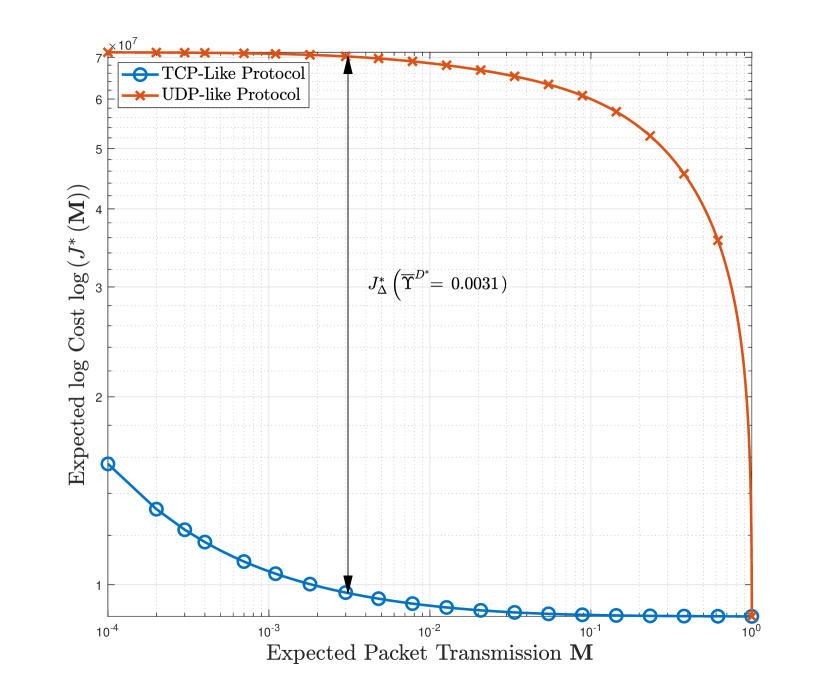
Figure 3: The log cost plot of the TCP-like and the UDP-like protocols for the inverted pendulum system seen in [5]. The mean of the packet transmission variable, ${\bf{V}}_{k}$, is varied over the $\left[0,1\right]$ region.

The cost difference of the two protocols arises from different control laws. Table I shows the closed loop eigenvalues of the TCP-like and the UDP-like protocols. Where the closed loop gain ${\bf K}_{{\cal I}_{k}}$ is defined as the first $m$ by $n$ block of the matrix ${\bf G}_{{\cal I}_{k}}\Omega_{gp}~{}$. Additionally, the packet transmission variable is set at $\ \!\!\overline{\Upsilon}\!\!\ =0.9$ for the calculation of the closed loop eigenvalues. As shown in Table I, the TCP-like protocol has a conjugate pair of eigenvalues with a smaller complex component when compared to the UDP-like eigenvalues. This suggests the damping of the state response is lower for the UDP-like protocol than the TCP-like protocol. Additionally, the magnitude of the TCP complex-conjugate eigenvalues is closer to the origin, this points to faster decay in the response of these modes.

TABLE I: Closed Loop Eigenvalues of (101)

$\lambda_{i}({\bf A}-{\bf B}{\bf K}_{{\cal I}_{k}})$	TCP-like Eigenvalues	UDP-like Eigenvalues
$\lambda_{1}$	$0.9497+0.0056i$	$0.9907+0.0201i$
$\lambda_{2}$	$0.9497-0.0056i$	$0.9907-0.0201i$
$\lambda_{3}$	$-0.1148$	$0.9729$
$\lambda_{4}$	$0.9978$	$0.9382$

V-B Multiple Actuator System

For the second case study we consider an arbitrary system with multiple actuators. This system is constructed as,

$${\bf A}\mkern-18.0mu\ = \mkern-18.0mu\ \left(\!\!\begin{array}[]{cc}1.03&0.005\\ 0.35&1.01\end{array}\!\!\right),\quad{\bf B}=\left(\!\!\begin{array}[]{cc}1&0\\ 0&1\end{array}\!\!\right),$$ (102e)

$$\Psi\mkern-18.0mu\ = \mkern-18.0mu\ {\bf I}_{N}\otimes\left(\!\!\begin{array}[]{cc}1&0\\ 0&1\end{array}\!\!\right),\quad\ \ \ \Omega={\bf I}_{N}\otimes\left(\!\!\begin{array}[]{cc}1&0\\ 0&1\end{array}\!\!\right),$$ (102j)

and the prediction horizon is set to $N=10$. The system in (102) has multiple actuators and thus is used to highlight the generality of our results.

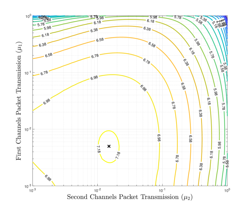
Figure 4: The log cost contour plot of the difference in cost of the UDP-like and the TCP-like protocol for the system (102). The mean of the packet transmission variable, ${\bf M}$, is varied over the $\left[0,1\right]^{2}$ region. The point of maximal cost difference is marked with a black cross.

The expected cost difference, as seen in Fig. 4, shows existence of a maximal point despite the system having multiple actuators, as predicted by Theorem 2. This is marked with a black cross in Fig. 4. This indicates that the results extend to multiple actuators. Fig. 4 shows that the cost difference is strictly positive when ${\bf M}\neq{\bf I}$ and ${\bf M}\neq{\bf 0}$.

When considering the expected cost for this system, the presence of a second actuator means the expected cost is a function of multiple packet transmission variables. As a result, there are regions within $\left[0,1\right]^{2}$ where the expected cost remains fixed for a range of values of ${\bf M}$. This behaviour is depicted in Fig. 5 and Fig. 6 for the TCP-like and UDP-like expected costs, respectively.

TABLE II: Closed Loop Eigenvalues of (102)

$\lambda_{i}({\bf A}-{\bf B}{\bf K}_{{\cal I}_{k}})$	TCP-like Eigenvalues	UDP-like Eigenvalues
$\lambda_{1}$	$-0.1082$	$0.4904+0.0312i$
$\lambda_{2}$	$-0.8938$	$0.4904-0.0312i$

As mentioned for the previous case study, the control laws developed in Section III are different for each protocol. As shown in Table II, the UDP-like protocol has a complex conjugate pair of eigenvalues. Note that for the purposes of calculating the eigenvalues in Table II, the communication channel is not a scalar, in fact we set ${\bf M}=\leavevmode\hbox{\set@color$\left(\begin{smallmatrix}0.9&0\\ 0&0.5\end{smallmatrix}\right)$}$. As with the pendulum case study it is seen that the TCP-like and the UDP-like control laws induce different behaviour in the state trajectories.

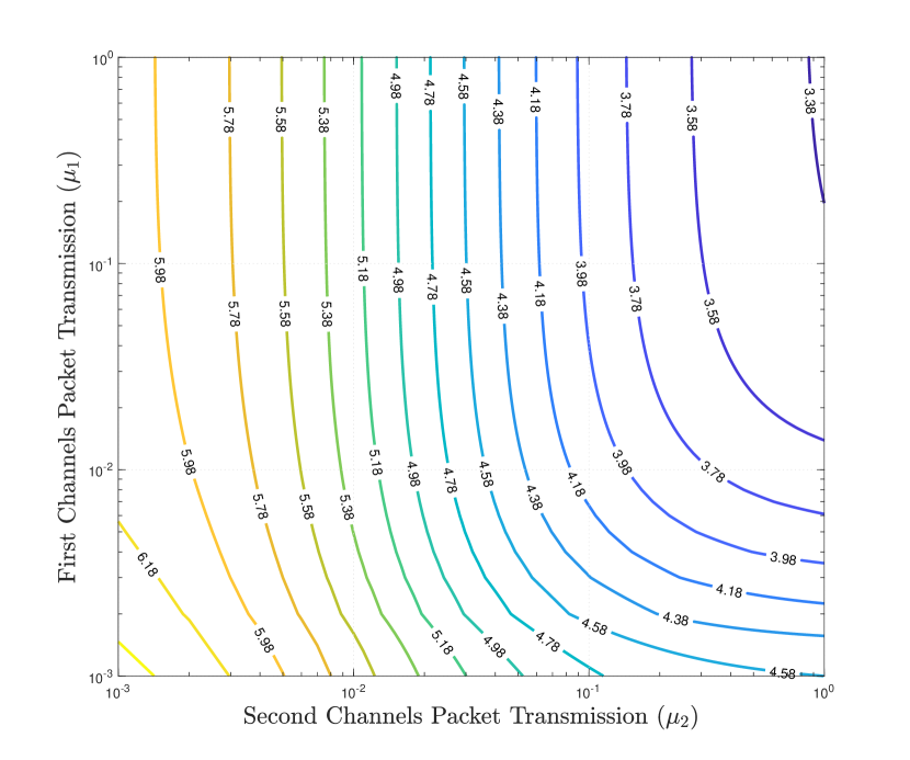
Figure 5: The log expected cost contour plot of the TCP-like protocol for the system (102). The mean of the packet transmission variable, ${\bf M}$, is varied over the $\left[0,1\right]^{2}$ region.

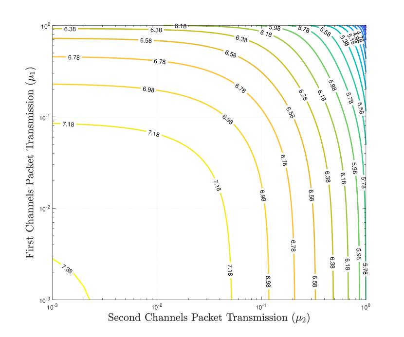
Figure 6: The log expected cost contour plot of the UDP-like protocol for the system (102). The mean of the packet transmission variable, ${\bf M}$, is varied over the $\left[0,1\right]^{2}$ region.

VI Packet Loss Allocation Optimisation

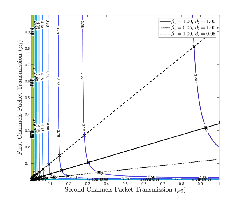
Figure 7: The log expected cost contour plot of the TCP-like protocol for the system (102). The mean of the packet transmission variable, ${\bf M}$, is varied over the $\left[0,1\right]^{2}$ region.

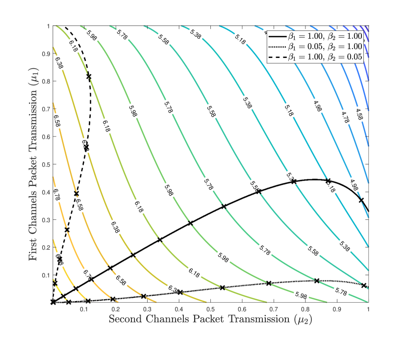
Figure 8: The log expected cost contour plot of the UDP-like protocol for the system (102). The mean of the packet transmission variable, ${\bf M}$, is varied over the $\left[0,1\right]^{2}$ region.

In modern communication systems, the probability of packet loss is determined by the performance of multiple processes. These processes range from the modulation and coding, which operate in the lower layers, to the routing and flow control, operating in the higher layers. While characterising the probability of packet transmission of a modern communication system is challenging in general, the probability of packet transmission decreases monotonically [14] with the resources allocated to the communication system, i.e. bandwidth, power, and delay. Indeed, resource allocation is a fundamental problem in communication systems and is often confronted with competing objectives for which the efficiency tradeoffs are difficult to describe analytically. In our setting, the extension to the multidimensional actuation channel poses a central question that concerns the design of the communication system of the control system, namely the optimal allocation of communication resources to each of the actuation channel dimensions. In the following, we capitalise on the analytical framework developed above and provide a resource allocation framework that optimises the packet loss probabilities for each actuation dimension while satisfying a total budget constraint.

The set of packet loss probability matrices that achieve a given cost $\alpha\in\mathds{R}_{+}$ is the set of channel matrices described by

$${\cal M}_{k}\left(\!{\cal I}_{k}\!\right)=\left\{{\bf M}:J^{*}\left(\!{\cal I}_{k}\!\right)\leq\alpha\right\}.$$ (103)

All the matrices in the set induce a control cost that is upper bounded by $\alpha$ but differ in their use of communication resources, i.e. the packet transmission performance across different dimensions. To quantify the use of communication resources in global terms, a communication cost for the system is proposed, defined as

$$C\left({\bf M}\right)\stackrel{{\scriptstyle\Delta}}{{=}}\sum\limits_{i=1}^{m}\beta_{i}\mu_{i}=\textnormal{tr}\left(\bm{\beta}{\bf M}\right),$$ (104)

where $\bm{\beta}\in{\bf S}^{+}_{m\times m}$ is the non-negative definite penalty matrix where each diagonal entry, $\beta_{i}\in\mathds{R}$, is a penalty term corresponding to the cost of communication in that channel. The communication cost captures the notion of a total communication budget for the system. That being the case, the minimum communication cost is defined as

$$C_{\alpha}\left(\!{\cal I}_{k}\!\right)\stackrel{{\scriptstyle\Delta}}{{=}}\operatorname*{arg\,min}\limits_{{\bf M}\in{\cal M}_{k}\left(\!{\cal I}_{k}\!\right)}\ C\left({\bf M}\right).$$ (105)

The maximum channel efficiency yields a communication setup that minimises the total number of packet losses while maintaining the system control performance. In view of this, the communication system configuration that minimises the amount of resources allocated to the actuation channel is

$${\bf M}^{*}\stackrel{{\scriptstyle\Delta}}{{=}}\min\limits_{{\bf M}\in{\cal M}_{k}\left(\!{\cal I}_{k}\!\right)}\ C\left({\bf M}\right).$$ (106)

This cost of communication formulation highlights the importance of Corollary 2. Specifically, if it is costly to communicate over a particular dimension then allocating as few resources as possible whilst maintaining a desired control cost is desirable, indeed, as few resources as dictated by the minimiser ${\bf M}^{*}$.

The optimisation of the communication channel for the pendulum case study presented in Section V-A is straightforward. There is a single communication channel, and therefore, the maximum channel efficiency is the packet transmission value that achieves the optimal control cost of $\alpha$ with equality. However, for the system presented in Section V-B(102) there are fixed regions of expected cost for both the TCP-like protocol and the UDP-like protocol, as shown in Fig. 7 and Fig. 8, respectively. The black dashed lines plotted in Fig. 7 and Fig. 8 correspond to the channel matrices defined in (106) that achieve the maximum channel efficiency. The values of $\beta$ are selected for three different cases. For the first case the cost is symmetric in both channel dimensions, i.e. $\beta$ is set to ${\bf I}$ and for the second and third cases the entries are set to $(0.05,1)$ and $(1,0.05)$, respectively. These cases model the situation in which communication across one of the channel dimensions induces larger cost. Additionally, we also mark the optimal allocation points for each contour line with a black cross. The same weighting matrices are used for both the UDP-like and the TCP-like figures. Note that for the point at which the minimum communication cost is achieved by a matrix ${\bf M}^{*}$ with either $\mu_{1}=1$ or $\mu_{2}=1$, the optimisation for the channel reduces to the single dimensional case, i.e. one of the channel dimensions is perfect and the other dimension incurs in all packet loss. Furthermore, Fig. 8 shows that for all the three weightings of the channel cost considered, the maximum channel efficiency for $\alpha\geq 4.78$ requires at least one of the channels to be perfect.

The packet loss allocation presented above is not possible with the results [5], due to the scalar channel model.

VII Conclusion

This paper extends existing results in the literature from a scalar channel to the multidimensional channel and, in doing so, derive a proof of the optimal control law for the TCP-like and UDP-like protocols. Additionally, an analytic proof is provided showing that the UDP-like LQG expected cost is strictly greater than the TCP-like expected cost. It is also shown that the cost is monotonically decreasing in the packet transmission variable. The proofs provided are also valid for non-stationary sequences of packet loss. This extension is shown by minor adjustments in the conditions. The maximal cost difference is shown to exist within the $\left[0,1\right]$ region. As seen in Fig. 4, this maximal cost difference exists in the higher dimensional communication channel. In showing that the TCP-like protocol outperforms the UDP-like protocol, in terms of LQG cost for all values of ${\bf 0\prec{\bf M}\prec I}~{}$ it has highlighted the problem of deciding which protocol to use. The discussion of channel cost optimisation began in Section VI, however, implementing the TCP-like protocol on a system requires the existence of a perfect acknowledgement link. The cost of introducing this communication link is not included in the communication cost design. The trade-off between choosing the UDP-like or the TCP-like protocol for a particular system must take this additional cost into account.

Lemma 1

Consider the system modelled by (1) with access to (2). Then the following holds

$$\mbox{\bb E}\left[{\bf E}_{k}^{\sf T}\Omega{{\bf E}_{k}}{\Big{|}}{\cal F}_{k}\right]\mkern-18.0mu = \mkern-18.0mu\ \textnormal{tr}\left(\Omega_{l}\Sigma_{\pazocal{W}}\right),$$ (107a)

$$\hfill\mbox{\bb E}\left[{\bf E}_{k}^{\sf T}\Omega{{\bf E}_{k}}{\Big{|}}{\cal G}_{k}\right]\mkern-18.0mu = \mkern-18.0mu{\pazocal{U}_{k}\!\!\left(\!{\cal G}_{k}\!\right)\!^{\sf T}}\ \!\!\overline{\Upsilon}\!\!\ \left({\bf I}\!\odot\!\Omega_{g}\!\right)\!\!\left(\!{\bf I}-\!\!\ \!\!\overline{\Upsilon}\!\!\ \!\right){\pazocal{U}_{k}\!\!\left(\!{\cal G}_{k}\!\right)\!}$$ (107b)

$$\qquad\qquad\qquad\!\!+\textnormal{tr}\left(\Omega_{l}\Sigma_{\pazocal{W}}\right),$$

where $\Omega_{l}=\Lambda\Omega\Lambda$.

The proof is split into two parts, one for TCP-like protocol and one for the UDP-like protocol, respectively.

Proof:

-1 TCP-like protocol

The expected error in TCP-like follows from (64a). Substituting this into the left-hand side of (71a) yields

$$\mbox{\bb E}\left[{\bf E}_{k}^{\sf T}\Omega{{\bf E}_{k}}{\Big{|}}{\cal F}_{k}\right] = \mbox{\bb E}\left[{\pazocal{W}}_{k}^{\sf T}\Omega_{l}{\pazocal{W}}_{k}{\Big{|}}{\cal F}_{k}\right],$$ (108)

$$= \textnormal{tr}\left(\Omega_{l}\Sigma_{\pazocal{W}}\right).$$ (109)

This completes the TCP-like part of the proof.

-2 UDP-like protocol

The error in UDP-like estimation follows from (64b). Substituting this into the left-hand side of (71b) gives

$$\mkern-36.0mu\mbox{\bb E}\left[{{\bf E}^{{}^{\sf T}}_{k}}\Omega{{\bf E}_{k}}{\Big{|}}{\cal G}_{k}\right]=\mbox{\bb E}\left[{\pazocal{U}_{k}}^{\sf T}\left(\ \!\!\Upsilon_{k}\!\!\ -\ \!\!\overline{\Upsilon}\!\!\ \right)\Omega_{g}\left(\ \!\!\Upsilon_{k}\!\!\ -\ \!\!\overline{\Upsilon}\!\!\ \right){\pazocal{U}_{k}}{\Big{|}}{\cal G}_{k}\right]$$

$$\qquad\qquad\qquad\qquad\qquad+\mbox{\bb E}\left[{\pazocal{W}}_{k}^{\sf T}\Lambda\Omega{\Lambda{\pazocal{W}}_{k}}{\Big{|}}{\cal G}_{k}\right],$$

where we use the fact that ${\pazocal{W}}_{k}$ is zero mean to eliminate the cross terms. Note that the second term is identical to the TCP-like case, as seen in (108). Therefore,

$$\mkern-36.0mu\mbox{\bb E}\left[{\bf E}_{k}^{\sf T}\Omega{{\bf E}_{k}}{\Big{|}}{\cal G}_{k}\right]=\mbox{\bb E}\left[{\pazocal{U}_{k}}^{\sf T}\ \!\!\Upsilon_{k}\!\!\ \Omega_{g}{\ \!\!\Upsilon_{k}\!\!\ }{\pazocal{U}_{k}}{\Big{|}}{\cal G}_{k}\right]$$

$$\qquad\qquad\qquad-{\pazocal{U}_{k}\!\!\left(\!{\cal G}_{k}\!\right)\!^{\sf T}}\ \!\!\overline{\Upsilon}\!\!\ \Omega_{g}\ \!\!\overline{\Upsilon}\!\!\ {\pazocal{U}_{k}\!\!\left(\!{\cal G}_{k}\!\right)\!}+\textnormal{tr}\left(\Omega_{l}\Sigma_{\pazocal{W}}\right).$$

It follows from Lemma 4 in the Appendix that

$$\mbox{\bb E}\!\left[\!\left.{\bf E}_{k}^{\sf T}\!\Omega{{\bf E}_{k}}\right|{\cal G}_{k}\!\right]\!\!\!=\pazocal{U}_{k}\!\!\left(\!{\cal G}_{k}\!\right)\!^{\sf T}\!\ \!\!\overline{\Upsilon}\!\!\ \!\!\left({\bf I}\odot\Omega_{g}\!\right)\!\!\!\left({\bf I}-\ \!\!\overline{\Upsilon}\!\!\ \right)\!\!{\pazocal{U}_{k}\!\!\left(\!{\cal G}_{k}\!\right)\!}+\textnormal{tr}\left(\Omega_{l}\Sigma_{\pazocal{W}}\!\right)\!\!.$$

This concludes the proof. ∎

Lemma 4

It is proved that:

$$\mkern-36.0mu\mkern-18.0mu\mbox{\bb E}\left[{\pazocal{U}_{k}}^{\sf T}\ \!\!\Upsilon_{k}\!\!\ ^{{}^{\sf T}}\Omega_{g}\ \!\!\Upsilon_{k}\!\!\ {\pazocal{U}_{k}}{\Big{|}}{\cal G}_{k}\right]={\pazocal{U}_{k}\!\!\left(\!{\cal G}_{k}\!\right)\!}^{\sf T}\ \!\!\overline{\Upsilon}\!\!\ \Omega_{g}\ \!\!\overline{\Upsilon}\!\!\ {\pazocal{U}_{k}\!\!\left(\!{\cal G}_{k}\!\right)\!}$$

$$\qquad\qquad+{\pazocal{U}_{k}\!\!\left(\!{\cal G}_{k}\!\right)\!}^{\sf T}\ \!\!\overline{\Upsilon}\!\!\ \left({\bf I}\!\odot\!\Omega_{g}\!\right)\!\!\left(\!{\bf I}-\!\!\ \!\!\overline{\Upsilon}\!\!\ \!\right){\pazocal{U}_{k}\!\!\left(\!{\cal G}_{k}\!\right)\!},$$ (110)

where ${\bf I}$ is the identity matrix and $\odot$ is the element wise Hadamard product.

Proof:

The left hand side of (110) is scalar, and therefore

$$\mkern-36.0mu\!\!\mbox{\bb E}\!\!\left[\pazocal{U}_{k}\!\!\left(\!{\cal G}_{k}\!\right)\!^{\sf T}\ \!\!\Upsilon_{k}\!\!\ ^{\sf T}\Omega_{g}\ \!\!\Upsilon_{k}\!\!\ {\pazocal{U}_{k}\!\!\left(\!{\cal G}_{k}\!\right)\!^{\sf T}}{\Big{|}}{\cal G}_{k}\right]$$

$$\mkern-36.0mu\mkern-18.0mu\ =\!\mbox{\bb E}\!\!\left[\!U_{0}\!\!\left(\!{\cal G}_{k}\!\right)\!\!{\bf V}_{0}\Omega_{g_{(1,1)}}\!\!\!\!{\bf V}_{0}U_{0}\!\!\left(\!{\cal G}_{k}\!\right)\!\!{\Big{|}}\!{\cal G}_{k}\!\!\right]\!\!+\!\mbox{\bb E}\!\!\left[\!U_{0}\!\!\left(\!{\cal G}_{k}\!\right)\!{\bf V}_{0}\Omega_{g_{(1,2)}}\!\!\!\!{\bf V}_{1}U_{1}\!\!\left(\!{\cal G}_{k}\!\right)\!\!{\Big{|}}\!{\cal G}_{k}\!\!\right]$$

$$\mkern-36.0mu\dots\ +\mbox{\bb E}\left[U_{Nm-1}\!\!\left(\!{\cal G}_{k}\!\right)\!\!{\bf V}_{Nm-1}\Omega_{g_{(Nm,Nm)}}{\bf V}_{Nm-1}U_{Nm-1}\!\!\left(\!{\cal G}_{k}\!\right)\!\!{\Big{|}}{\cal G}_{k}\right],$$

$$= \mkern-18.0mu\sum\limits_{i=1}^{Nm}\left(U_{i-1}\!\!\left(\!{\cal G}_{k}\!\right)\!{\bf M}_{i-1}\Omega_{g_{(i,i)}}U_{i-1}\!\!\left(\!{\cal G}_{k}\!\right)\!\!\vphantom{\sum\limits_{j=1,j\neq i}^{Nm}}\right.$$

$$\left.+\sum\limits_{j=1,j\neq i}^{Nm}U_{i-1}\!\!\left(\!{\cal G}_{k}\!\right)\!{\bf M}_{i-1}\Omega_{g_{(i,j)}}{\bf M}_{j-1}U_{j-1}\!\!\left(\!{\cal G}_{k}\!\right)\!\!,\right)$$

$$= \mkern-18.0mu\sum\limits_{i=1}^{Nm}\sum\limits_{j=1}^{Nm}U_{i-1}\!\!\left(\!{\cal G}_{k}\!\right)\!\!{\bf M}_{i-1}\Omega_{g_{(i,i)}}\left(1-{\bf M}_{i-1}\right)U_{i-1}\!\!\left(\!{\cal G}_{k}\!\right)\!\!$$

$$\qquad+U_{i-1}\!\!\left(\!{\cal G}_{k}\!\right)\!\!{\bf M}_{i-1}\Omega_{g_{(i,j)}}{\bf M}_{j-1}U_{j-1}\!\!\left(\!{\cal G}_{k}\!\right)\!\!,$$

$$= \mkern-18.0mu{\pazocal{U}_{k}\!\!\left(\!{\cal G}_{k}\!\right)\!}^{\sf T}\ \!\!\overline{\Upsilon}\!\!\ \!\left({\bf I}\!\odot\!\Omega_{g}\!\right)\!\!\left(\!{\bf I}-\!\!\ \!\!\overline{\Upsilon}\!\!\ \!\right){\pazocal{U}_{k}\!\!\left(\!{\cal G}_{k}\!\right)\!}+{\pazocal{U}_{k}\!\!\left(\!{\cal G}_{k}\!\right)\!}^{\sf T}\ \!\!\overline{\Upsilon}\!\!\ \Omega_{g}\!\!\ \!\!\overline{\Upsilon}\!\!\ {\pazocal{U}_{k}\!\!\left(\!{\cal G}_{k}\!\right)\!},$$

where bracketed subscripts represent the $(i,j)$-th element. This concludes the proof. ∎

Theorem 1

Consider the closed-loop systems shown in Fig. 1 and Fig. 2, with plant dynamics given in (1), protocol dependent information sets given in (2) and controller cost function given in (II). Then the optimal cost for the TCP-like protocol is

$$J^{*}\left({\cal F}_{k}\right)=\!\!X_{k}^{\sf T}\!\!\left({\bf Q}+\Omega_{p}\right)\!\!X_{k}\!+\!\textnormal{tr}\left(\Sigma_{\pazocal{W}}\Omega_{l}\!\right)\!\!-\!X_{k}^{\sf T}\!{\bf F}^{\sf T}\!\!{\bf G}^{\scalebox{0.5}[1.0]{$-$}1}\!\!\left(\!{\cal F}_{k}\!\right)\!\!\ \!\!\overline{\Upsilon}\!\!\ {\bf F}X_{k},$$

and the optimal cost for the UDP-like protocol is

$$J^{*}\left({\cal G}_{k}\right)=\!\!X_{k}^{\sf T}\!\!\left({\bf Q}+\Omega_{p}\right)\!\!X_{k}\!+\!\textnormal{tr}\left(\Sigma_{\pazocal{W}}\Omega_{l}\!\right)\!\!-\!X_{k}^{\sf T}\!{\bf F}^{\sf T}\!\!{\bf G}^{\scalebox{0.5}[1.0]{$-$}1}\!\!\left(\!{\cal G}_{k}\!\right)\!\!\ \!\!\overline{\Upsilon}\!\!\ {\bf F}X_{k}.$$

As with Lemma 1 the proof is split into two parts to account for the two protocols.

Proof:

-1 Optimal Cost for the TCP-like Protocol

Substituting (71a) into (70), noting that under the TCP-like protocol the error term does not depend on $\pazocal{U}_{k}$, gives

$$J^{*}\!\!\left(\!{\cal F}_{k}\!\right)\mkern-18.0mu = \mkern-18.0muX_{k}^{\sf T}\!\left({\bf Q}+\Omega_{p}\right)X_{k}+\textnormal{tr}\left(\Omega_{l}\Sigma_{\pazocal{W}}\right)$$ (111)

$$\mkern-36.0mu+\min_{\pazocal{U}_{k}\!\!\left(\!{\cal G}_{k}\!\right)}\!\left\{\!\pazocal{U}_{k}\!\!\left(\!{\cal G}_{k}\!\right)\!^{\sf T}\ \!\!\overline{\Upsilon}\!\!\ \!\!\left(2{\bf F}X_{k}\!+\!\left(\Omega_{g}\ \!\!\overline{\Upsilon}\!\!\ \!+\!\Psi\right){\pazocal{U}_{k}\!\!\left(\!{\cal G}_{k}\!\right)\!}\right)\right\}\!\!.$$

Note that $\left(\Omega_{g}\ \!\!\overline{\Upsilon}\!\!\ +\Psi\right)$ is positive definite, and therefore, (111) is convex. Taking the derivative of the cost with respect to ${\pazocal{U}_{k}}$ yields

$${{\partial J^{*}\left({\cal F}_{k}\right)}\over{\partial{\pazocal{U}_{k}}}}=2\ \!\!\overline{\Upsilon}\!\!\ \left({\bf F}X_{k}+\left(\Omega_{g}\ \!\!\overline{\Upsilon}\!\!\ +\Psi\right){\pazocal{U}_{k}\!\!\left(\!{\cal F}_{k}\!\right)\!}\right).$$ (112)

Solving for all $\ \!\!\overline{\Upsilon}\!\!\ \neq{\bf 0}$, the minimising value of ${\pazocal{U}_{k}\!\!\left(\!{\cal F}_{k}\!\right)\!}$ is found to be

$$\pazocal{U}_{k}^{*}\!\!\left(\!{\cal F}_{k}\!\right)\!\stackrel{{\scriptstyle\Delta}}{{=}}-\left(\Omega_{g}\ \!\!\overline{\Upsilon}\!\!\ +\Psi\right)^{\scalebox{0.5}[1.0]{$-$}1}{\bf F}X_{k}.$$ (113)

Denoting $\left(\Omega_{g}\ \!\!\overline{\Upsilon}\!\!\ +\Psi\right)$ by ${\bf G}^{\scalebox{0.5}[1.0]{$-$}1}\!\!\left(\!{\cal F}_{k}\!\right)\!$ and substituting ${\Upsilon_{k|\mathcal{F}_{k}}^{*}}$ into (111) results in the optimal expected cost for the operator, described by

$$J^{*}\left({\cal F}_{k}\right)=\!\!X_{k}^{\sf T}\!\!\left({\bf Q}+\Omega_{p}\right)\!\!X_{k}\!+\!\textnormal{tr}\left(\Sigma_{\pazocal{W}}\Omega_{l}\!\right)\!\!-\!X_{k}^{\sf T}\!{\bf F}^{\sf T}\!\!{\bf G}^{\scalebox{0.5}[1.0]{$-$}1}\!\!\left(\!{\cal F}_{k}\!\right)\!\!\ \!\!\overline{\Upsilon}\!\!\ {\bf F}X_{k}.$$

This concludes the TCP-like part of the proof.

-2 Optimal Cost for the UDP-like Protocol

Combining (71b) and (70) the optimal cost function for the UDP-like protocol is given by:

$$\mkern-18.0muJ^{*}\left({\cal G}_{k}\right)=X_{k}^{\sf T}\left({\bf Q}+\Omega_{p}\right)X_{k}+\textnormal{tr}\left(\Omega_{l}\Sigma_{\pazocal{W}}\right)$$

$$\mkern-36.0mu+\min_{\pazocal{U}_{k}\!\!\left(\!{\cal G}_{k}\!\right)}\!\left\{\!\pazocal{U}_{k}\!\!\left(\!{\cal G}_{k}\!\right)\!^{\sf T}\!\ \!\!\overline{\Upsilon}\!\!\ \!\!\left(\!2{\bf F}X_{k}\!+\!\left(\!\Omega_{g}\!\!\ \!\!\overline{\Upsilon}\!\!\ \!\!+\!\Psi\!+\!\!\left({\bf I}\!\odot\!\Omega_{g}\!\right)\!\!\left(\!{\bf I}-\!\!\ \!\!\overline{\Upsilon}\!\!\ \!\right)\!\!\right)\!\!{\pazocal{U}_{k}\!\!\left(\!{\cal G}_{k}\!\right)\!}\right)\!\!\right\}\!\!.$$

Following the same process as with the TCP-like case, noting that $\left(\Omega_{g}\ \!\!\overline{\Upsilon}\!\!\ \!+\!\Psi+\left({\bf I}\!\odot\!\Omega_{g}\!\right)\!\!\left(\!{\bf I}-\!\!\ \!\!\overline{\Upsilon}\!\!\ \!\right)\right)$ is positive definite, and therefore the minimisation is convex yields

$${{\partial J^{*}\!\left(\!{\cal G}_{k}\!\right)}\over{\partial{\pazocal{U}_{k}}}}=2\ \!\!\overline{\Upsilon}\!\!\ \!\!\left({\bf F}X_{k}\!+\!\left(\Omega_{g}\ \!\!\overline{\Upsilon}\!\!\ \!+\!\Psi+\left({\bf I}\!\odot\!\Omega_{g}\!\right)\!\!\left(\!{\bf I}-\!\!\ \!\!\overline{\Upsilon}\!\!\ \!\right)\!\right){\pazocal{U}_{k}\!\!\left(\!{\cal G}_{k}\!\right)\!}\right),$$

meaning that the optimal value of $\pazocal{U}_{k}^{*}\!\!\left(\!{\cal G}_{k}\!\right)\!$ is

$${\pazocal{U}_{k}^{*}\!\!\left(\!{\cal G}_{k}\!\right)\!}\stackrel{{\scriptstyle\Delta}}{{=}}-\left(\Psi+\left({\bf I}\!\odot\!\Omega_{g}\!\right)\!\!\left(\!{\bf I}-\!\!\ \!\!\overline{\Upsilon}\!\!\ \!\right)+\Omega_{g}\ \!\!\overline{\Upsilon}\!\!\ \right)^{\scalebox{0.5}[1.0]{$-$}1}{\bf F}X_{k}.$$ (114)

Re-labelling $\left(\Psi+\left({\bf I}\!\odot\!\Omega_{g}\!\right)\!\!\left(\!{\bf I}-\!\!\ \!\!\overline{\Upsilon}\!\!\ \!\right)+\Omega_{g}\ \!\!\overline{\Upsilon}\!\!\ \right)$ as ${\bf G}\!\!\left(\!{\cal G}_{k}\!\right)\!$ and substituting ${\pazocal{U}_{k}^{*}\!\!\left(\!{\cal G}_{k}\!\right)\!}$ into (111) yields the optimal expected cost for the operator:

$$J^{*}\left({\cal G}_{k}\right)=\!\!X_{k}^{\sf T}\!\!\left({\bf Q}+\Omega_{p}\right)\!\!X_{k}\!+\!\textnormal{tr}\left(\Sigma_{\pazocal{W}}\Omega_{l}\!\right)\!\!-\!X_{k}^{\sf T}\!{\bf F}^{\sf T}\!\!{\bf G}^{\scalebox{0.5}[1.0]{$-$}1}\!\!\left(\!{\cal G}_{k}\!\right)\!\!\ \!\!\overline{\Upsilon}\!\!\ {\bf F}X_{k}.$$ (115)

This concludes the proof. ∎

Lemma 2

The cost difference between the UDP-like and the TCP-like protocols is defined as

$$J_{\Delta}^{*}\left(\ \!\!\overline{\Upsilon}\!\!\ \right)\stackrel{{\scriptstyle\Delta}}{{=}}J^{*}\left({\cal G}_{k}\right)-J^{*}\left({\cal F}_{k}\right) > 0.$$ (116)

The derivative of this cost difference is

$${{\partial J_{\Delta}^{*}\left(\ \!\!\overline{\Upsilon}\!\!\ \right)}\over{\partial\ \!\!\overline{\Upsilon}\!\!\ }}\mkern-18.0mu = \mkern-18.0muX_{k}^{\sf T}{\bf F}^{\sf T}\left({\bf G}^{\scalebox{0.5}[1.0]{$-$}1}\!\!\left(\!{\cal G}_{k}\!\right)\!\left(\vphantom{\Big{|}}\left(1-2\ \!\!\overline{\Upsilon}\!\!\ \right)\Omega_{d}\right.\right.$$ (117)

$$\mkern-36.0mu\mkern-36.0mu\mkern-36.0mu\ \ \left.\left.-\ \!\!\overline{\Upsilon}\!\!\ \!\!\left(\!\!1\scalebox{0.5}[1.0]{$-$}\!\!\ \!\!\overline{\Upsilon}\!\!\ \!\right)\!\!\!\left[\!\Omega_{h}{\bf G}^{\scalebox{0.5}[1.0]{$-$}1}\!\!\left(\!{\cal G}_{k}\!\right)\!\Omega_{d}+\Omega_{d}{\bf G}^{\scalebox{0.5}[1.0]{$-$}1}\!\!\left(\!{\cal F}_{k}\!\right)\!\Omega_{g}\right]\!\right)\!\!{\bf G}^{\scalebox{0.5}[1.0]{$-$}1}\!\!\left(\!{\cal F}_{k}\!\right)\!\right)\!\!{\bf F}X_{k}\!,\quad\$$

where $\Omega_{d}=\left({\bf I}\odot\Omega_{g}\right)$ and $\ \!\!\overline{\Upsilon}\!\!\ \in\left[0,1\right]$.

Proof:

In order to proceed with the proof we analyse the matrices ${\bf G}^{\scalebox{0.5}[1.0]{$-$}1}\!\!\left(\!{\cal F}_{k}\!\right)\!$ and ${\bf G}^{\scalebox{0.5}[1.0]{$-$}1}\!\!\left(\!{\cal G}_{k}\!\right)\!$. We define the mappings ${\bf G}_{{\bf F}}\left(\alpha\right):\mathds{R}\rightarrow\mathds{R}^{n\times n}$ and ${\bf G}_{{\bf G}}\left(\alpha\right):\mathds{R}\rightarrow\mathds{R}^{n\times n}$ as

$${\bf G}_{{\bf F}}\left(\alpha\right) = \left(\alpha\Omega_{g}+\Psi\right)^{\scalebox{0.5}[1.0]{$-$}1},$$ (118a)

$${\bf G}_{{\bf G}}\left(\alpha\right) = \left(\alpha\Omega_{h}+\Omega_{d}+\Psi\right)^{\scalebox{0.5}[1.0]{$-$}1},$$ (118b)

where $\alpha\in\left[0,1\right]$, ${\bf G}_{{\bf F}}\!\!\left(\!\ \!\!\overline{\Upsilon}\!\!\ \!\right)\!\!={\bf G}^{\scalebox{0.5}[1.0]{$-$}1}\!\!\left(\!{\cal F}_{k}\!\right)\!$, $\!{\bf G}_{{\bf G}}\!\!\!\left(\!\ \!\!\overline{\Upsilon}\!\!\ \!\right)\!\!={\bf G}^{\scalebox{0.5}[1.0]{$-$}1}\!\!\left(\!{\cal G}_{k}\!\right)\!$, $\Omega_{d}=\left({\bf I}\odot\Omega_{g}\right)$, and $\Omega_{h}=\left(\Omega_{g}-\left({\bf I}\odot\Omega_{g}\right)\right)$. It should be noted that these two functions share the same inherent structure. Specifically, both of these functions are specialisations of the more general function

$${\bf G}_{\bf I}\left(\alpha,{\bf A},{\bf B}\right)=\left(\alpha{\bf A}+{\bf B}\right)^{\scalebox{0.5}[1.0]{$-$}1},$$ (119)

where ${\bf A}\in\mathds{R}^{nN\times nN}$, ${\bf B}\in\mathds{R}^{nN\times nN}$, and ${\bf G}_{\bf I}\left(\alpha,{\bf A},{\bf B}\right)$ is defined as the mapping ${\bf G}_{\bf I}\left(\alpha,{\bf A},{\bf B}\right):\mathds{R}\times\mathds{R}^{nN\times nN}\times\mathds{R}^{nN\times nN}\rightarrow\mathds{R}^{nN\times nN}$. This results in a single function that is equivalent to (118) where it is noted that ${\bf G}_{\bf I}\left(\alpha,\Omega_{g},\Psi\right)={\bf G}_{{\bf F}}\left(\alpha\right)$ and ${\bf G}_{\bf I}\left(\alpha,\Omega_{h},\left[\Omega_{d}+\Psi\right]\right)={\bf G}_{{\bf G}}\left(\alpha\right)$. Additionally, all inputs of the function ${\bf G}_{\bf I}\left(\alpha,{\bf A},{\bf B}\right)$ are symmetric and ${\bf B}$ is a diagonal positive definite matrix for both of the protocols considered. From this point, due to the fact that the matrices ${\bf A}$ and ${\bf B}$ are constants, we simplify the notation to ${\bf G}_{\bf I}\left(\alpha\right)$. Note that the results below apply to both the UDP-like and the TCP-like protocols. The function ${\bf G}_{\bf I}\left(\alpha\right)$ has a first derivative given by

$${{\partial}\over{\partial\beta}}{\bf G}_{\bf I}\left(\beta\right)\mkern-18.0mu\ = \mkern-18.0mu\ {{\partial}\over{\partial\beta}}\left(\beta{\bf A}+{\bf B}\right)^{\scalebox{0.5}[1.0]{$-$}1}$$ (120)

$$= \mkern-18.0mu\ \scalebox{0.75}[1.0]{$-$}\left(\beta{\bf A}+{\bf B}\right)^{\scalebox{0.5}[1.0]{$-$}1}\!\!\left[{{\partial}\over{\partial\beta}}\left(\beta{\bf A}+{\bf B}\right)\right]\!\!\left(\beta{\bf A}+{\bf B}\right)^{\scalebox{0.5}[1.0]{$-$}1}\!\!\!,\ \ \ \ \$$

where in (120) the derivative is recast according to [12, 17.3(a)]. Executing the derivative operator results in

$${{\partial}\over{\partial\beta}}{\bf G}_{\bf I}\left(\beta\right)\mkern-18.0mu\ = \mkern-18.0mu\ -{\bf G}_{\bf I}\left(\beta\right){\bf A}{\bf G}_{\bf I}\left(\beta\right).$$ (121)

With this in mind the derivative of the cost difference is computed to be

$$\mkern-18.0mu{{\partial J_{\Delta}^{*}\!\!\left(\!\ \!\!\overline{\Upsilon}\!\!\ \!\right)}\over{\partial\ \!\!\overline{\Upsilon}\!\!\ }}\mkern-18.0mu = \mkern-18.0mu\left[{{\partial}\over{\partial\ \!\!\overline{\Upsilon}\!\!\ }}\ \!\!\overline{\Upsilon}\!\!\ \left(1-\ \!\!\overline{\Upsilon}\!\!\ \right)\textnormal{tr}\left(\!{\bf G}_{{\bf G}}\!\!\!\left(\!\ \!\!\overline{\Upsilon}\!\!\ \!\right)\!\!\Omega_{d}{\bf G}_{{\bf F}}\!\!\left(\!\ \!\!\overline{\Upsilon}\!\!\ \!\right)\!\!{\bf L}\right)\right]\!\!,\!\!$$ (123)

$$= \mkern-18.0mu\left[{{\partial}\over{\partial\ \!\!\overline{\Upsilon}\!\!\ }}\ \!\!\overline{\Upsilon}\!\!\ \left(1-\ \!\!\overline{\Upsilon}\!\!\ \right)\right]\textnormal{tr}\left(\!{\bf G}_{{\bf G}}\!\!\!\left(\!\ \!\!\overline{\Upsilon}\!\!\ \!\right)\!\!\Omega_{d}{\bf G}_{{\bf F}}\!\!\left(\!\ \!\!\overline{\Upsilon}\!\!\ \!\right)\!\!{\bf L}\right)$$

$$\!\!\mkern-18.0mu+\ \!\!\overline{\Upsilon}\!\!\ \left(1-\ \!\!\overline{\Upsilon}\!\!\ \right)\textnormal{tr}\left(\left[{{\partial\!{\bf G}_{{\bf G}}\!\!\!\left(\!\ \!\!\overline{\Upsilon}\!\!\ \!\right)\!\!}\over{\partial\ \!\!\overline{\Upsilon}\!\!\ }}\right]\Omega_{d}{\bf G}_{{\bf F}}\!\!\left(\!\ \!\!\overline{\Upsilon}\!\!\ \!\right)\!\!{\bf L}\right)\!\!$$

$$\!\!\mkern-18.0mu+\ \!\!\overline{\Upsilon}\!\!\ \left(1-\ \!\!\overline{\Upsilon}\!\!\ \right)\textnormal{tr}\left(\!{\bf G}_{{\bf G}}\!\!\!\left(\!\ \!\!\overline{\Upsilon}\!\!\ \!\right)\!\!\Omega_{d}\left[{{\partial{\bf G}_{{\bf F}}\!\!\left(\!\ \!\!\overline{\Upsilon}\!\!\ \!\right)\!\!}\over{\partial\ \!\!\overline{\Upsilon}\!\!\ }}\right]{\bf L}\right)\!\!,\!\!$$

where in the third line the property [12, 17.5 pg.353] in conjunction with the product rule is utilised. At this stage, implementing the result seen in (121) yields

$$\mkern-18.0mu{{\partial J_{\Delta}^{*}\!\!\left(\!\ \!\!\overline{\Upsilon}\!\!\ \!\right)}\over{\partial\ \!\!\overline{\Upsilon}\!\!\ }}\mkern-18.0mu = \mkern-18.0mu\ X_{k}^{\sf T}{\bf F}^{\sf T}\left[{\bf G}_{{\bf G}}\!\!\left(\ \!\!\overline{\Upsilon}\!\!\ \right)\left[\left(1-2\ \!\!\overline{\Upsilon}\!\!\ \right)\Omega_{d}\right.\right.$$ (124)

$$\mkern-36.0mu\mkern-36.0mu\mkern-36.0mu\left.\left.-\ \!\!\overline{\Upsilon}\!\!\ \!\!\left(\!1\scalebox{0.5}[1.0]{$-$}\!\ \!\!\overline{\Upsilon}\!\!\ \!\right)\!\!\!\left[\Omega_{h}{\bf G}_{{\bf G}}\!\!\left(\ \!\!\overline{\Upsilon}\!\!\ \right)\Omega_{d}+\Omega_{d}{\bf G}_{{\bf F}}\!\!\left(\ \!\!\overline{\Upsilon}\!\!\ \right)\Omega_{g}\right]\right]{\bf G}_{{\bf F}}\!\!\left(\ \!\!\overline{\Upsilon}\!\!\ \right)\right]{\bf F}X_{k},$$

which corresponds to (91). This concludes the proof. ∎

Lemma 3

The relation

$${\hbox{det}}\left(\vphantom{\Big{|}}{\bf G}_{{\bf G}}\!\!\left(\ \!\!\overline{\Upsilon}\!\!\ \right)\left[\left(1-2\ \!\!\overline{\Upsilon}\!\!\ \right)\Omega_{d}\right.\right.$$

$$\mkern-36.0mu\mkern-36.0mu\left.\left.-\ \!\!\overline{\Upsilon}\!\!\ \!\!\left(\!1\scalebox{0.5}[1.0]{$-$}\!\ \!\!\overline{\Upsilon}\!\!\ \!\right)\!\!\!\left[\Omega_{h}{\bf G}_{{\bf G}}\!\!\left(\ \!\!\overline{\Upsilon}\!\!\ \right)\Omega_{d}+\Omega_{d}{\bf G}_{{\bf F}}\!\!\left(\ \!\!\overline{\Upsilon}\!\!\ \right)\Omega_{g}\right]\right]{\bf G}_{{\bf F}}\!\!\left(\ \!\!\overline{\Upsilon}\!\!\ \right)\vphantom{\Big{|}}\!\!\!\right)=0$$ (125)

has $2Nm$ many solutions, specifically,

$$\ \!\!\overline{\Upsilon}\!\!\ ^{D}_{2i-1} = {{1}\over{1+\sqrt{1+\lambda_{i}}}},$$ (126a)

$$\ \!\!\overline{\Upsilon}\!\!\ ^{D}_{2i} = {{1}\over{1-\sqrt{1+\lambda_{i}}}},$$ (126b)

where $\ \!\!\overline{\Upsilon}\!\!\ ^{D}_{i}$ correspondences to the $i$-th solution for (93) and $\lambda_{i}$ is the $i$-th eigenvalue of the matrix,

$$\left(\Omega_{g}\Omega_{d}^{\scalebox{0.5}[1.0]{$-$}1}\left(\Omega_{g}+\Psi\right)+\Psi\Omega_{d}^{\scalebox{0.5}[1.0]{$-$}1}\Omega_{h}\right)\left(\Omega_{g}+\Psi\right)^{\scalebox{0.5}[1.0]{$-$}1}\Omega_{d}\Psi^{\scalebox{0.5}[1.0]{$-$}1}.$$ (127)

Proof:

The first thing to establish is that the determinant of a matrix product is equal to the product of the respective matrix determinants [12, 4.31(a)]. Specifically, for any two matrices of equal dimensions

$${\hbox{det}}\left({\bf C}{\bf D}\right)={\hbox{det}}\left({\bf C}\right){\hbox{det}}\left({\bf D}\right).$$ (128)

Therefore, multiplying (93) from the left and right by ${\hbox{det}}\left(\Omega_{d}^{\scalebox{0.5}[1.0]{$-$}1}\right){\hbox{det}}\left({\bf G}_{{\bf G}}^{\scalebox{0.5}[1.0]{$-$}1}\left(\ \!\!\overline{\Upsilon}\!\!\ \right)\right)$ and ${\hbox{det}}\left({\bf G}_{{\bf F}}^{\scalebox{0.5}[1.0]{$-$}1}\left(\ \!\!\overline{\Upsilon}\!\!\ \right)\right){\hbox{det}}\left(\Omega_{d}^{\scalebox{0.5}[1.0]{$-$}1}\right)$ respectively gives

$${\hbox{det}}\!\!\left(\!\!\vphantom{\Big{|}}\left[\!\!\left(\!\!1\scalebox{0.5}[1.0]{$-$}2\!\ \!\!\overline{\Upsilon}\!\!\ \!\right)\!\!\Omega_{d}^{\scalebox{0.5}[1.0]{$-$}1}\!\scalebox{0.5}[1.0]{$-$}\!\ \!\!\overline{\Upsilon}\!\!\ \!\!\left(\!1\scalebox{0.5}[1.0]{$-$}\!\ \!\!\overline{\Upsilon}\!\!\ \!\right)\!\!\!\left[\Omega_{d}^{\scalebox{0.5}[1.0]{$-$}1}\!\Omega_{h}{\bf G}_{{\bf G}}\!\!\left(\!\ \!\!\overline{\Upsilon}\!\!\ \!\right)\!+\!{\bf G}_{{\bf F}}\!\!\left(\!\ \!\!\overline{\Upsilon}\!\!\ \!\right)\!\Omega_{g}\Omega_{d}^{\scalebox{0.5}[1.0]{$-$}1}\!\!\right]\!\right]\!\!\vphantom{\Big{|}}\right)\!\!=\!0\!.$$

Multiplying the left by ${\hbox{det}}\left({\bf G}_{{\bf F}}^{\scalebox{0.5}[1.0]{$-$}1}\left(\ \!\!\overline{\Upsilon}\!\!\ \right)\right)$ and the right by ${\hbox{det}}\left({\bf G}_{{\bf G}}^{\scalebox{0.5}[1.0]{$-$}1}\left(\ \!\!\overline{\Upsilon}\!\!\ \right)\right)$ and then re arranging yields

$$\mkern-36.0mu\mkern-36.0mu{\hbox{det}}\left(\vphantom{\Big{|}}\ \!\!\overline{\Upsilon}\!\!\ ^{2}\left[\Omega_{g}\Omega_{d}^{\scalebox{0.5}[1.0]{$-$}1}\left[\Omega_{g}+\Psi\right]+\Psi\Omega_{d}^{\scalebox{0.5}[1.0]{$-$}1}\Omega_{h}\right]\right.$$

$$\mkern-18.0mu\left.+2\ \!\!\overline{\Upsilon}\!\!\ \Psi\Omega_{d}^{\scalebox{0.5}[1.0]{$-$}1}\left(\Omega_{d}+\Psi\right)-\Psi\Omega_{d}^{\scalebox{0.5}[1.0]{$-$}1}\left(\Omega_{d}+\Psi\right)\vphantom{\Big{|}}\right)=0.$$ (129)

The above is a quadratic in the scalar, $\ \!\!\overline{\Upsilon}\!\!\$. However, it should be noted that due to the determinant this equation is actually of order $Nm$ in $\ \!\!\overline{\Upsilon}\!\!\$. To see this, note that $\ \!\!\overline{\Upsilon}\!\!\$ is pulled out of the determinant as follows

$$\mkern-36.0mu\mkern-36.0mu\ \!\!\overline{\Upsilon}\!\!\ ^{Nm}{\hbox{det}}\left(\vphantom{\Big{|}}-{{1}\over{\ \!\!\overline{\Upsilon}\!\!\ ^{2}}}\Psi\Omega_{d}^{\scalebox{0.5}[1.0]{$-$}1}\left(\Omega_{d}+\Psi\right)+2{{1}\over{\ \!\!\overline{\Upsilon}\!\!\ }}\Psi\Omega_{d}^{\scalebox{0.5}[1.0]{$-$}1}\left(\Omega_{d}+\Psi\right)\right.$$

$$\left.+\left[\Omega_{g}\Omega_{d}^{\scalebox{0.5}[1.0]{$-$}1}\left[\Omega_{g}+\Psi\right]+\Psi\Omega_{d}^{\scalebox{0.5}[1.0]{$-$}1}\Omega_{h}\right]\vphantom{\Big{|}}\right)=0.$$

Additionally, by assumption $\ \!\!\overline{\Upsilon}\!\!\ \neq 0$, therefore dividing by $-\ \!\!\overline{\Upsilon}\!\!\ ^{Nm}$ gives

$$\mkern-36.0mu\mkern-36.0mu{\hbox{det}}\left(\vphantom{{{1}\over{\ \!\!\overline{\Upsilon}\!\!\ ^{2}}}}\right.\left({{1}\over{\ \!\!\overline{\Upsilon}\!\!\ ^{2}}}-2{{1}\over{\ \!\!\overline{\Upsilon}\!\!\ }}\right)\underbrace{\left[\Psi\Omega_{d}^{\scalebox{0.5}[1.0]{$-$}1}\left(\Omega_{d}+\Psi\right)\right]}_{{\bf H}}$$

$$-\underbrace{\left[\Omega_{g}\Omega_{d}^{\scalebox{0.5}[1.0]{$-$}1}\!\!\left[\Omega_{g}+\Psi\right]+\Psi\Omega_{d}^{\scalebox{0.5}[1.0]{$-$}1}\!\!\Omega_{h}\right]}_{{\bf T}}\!\!{\left.\vphantom{{{1}\over{\ \!\!\overline{\Upsilon}\!\!\ ^{2}}}}\right)}\!\!=0.$$

From the above it is seen that the matrix ${\bf H}$ is positive definite and diagonal. Additionally, with some minor manipulation it is seen that ${\bf T}$ is symmetric. It is stated in [12, 16.51(c)] that there exists a matrix ${\bf S}\in\mathds{R}^{Nm\times Nm}$ such that ${\bf S}^{\bf T}{\bf H}{\bf S}={\bf I}$ and ${\bf S}^{\bf T}{\bf T}{\bf S}=\Lambda$. Therefore, multiplying the left and right by ${\hbox{det}}\left({\bf S}^{\bf T}\right)$ and ${\hbox{det}}\left({\bf S}\right)$ respectively gives

$${\hbox{det}}\left(\vphantom{{{1}\over{\ \!\!\overline{\Upsilon}\!\!\ ^{2}}}}{{1}\over{\ \!\!\overline{\Upsilon}\!\!\ ^{2}}}{\bf I}-2{{1}\over{\ \!\!\overline{\Upsilon}\!\!\ }}{\bf I}-\Lambda\right)\!\!=0,$$ (130)

where $\Lambda$ is the diagonal matrix where all diagonal entries, $\lambda_{i}$, are the eigenvalues of the matrix ${\bf T}{\bf H}^{\scalebox{0.5}[1.0]{$-$}1}$. The above is equivalent to

$$\prod_{i=1}^{Nm}\left({{1}\over{\ \!\!\overline{\Upsilon}\!\!\ ^{2}}}-2{{1}\over{\ \!\!\overline{\Upsilon}\!\!\ }}-\lambda_{i}\right)\!\!=0.$$ (131)

Note that (131) is $Nm$ polynomials on $\ \!\!\overline{\Upsilon}\!\!\$ with solutions

$$\ \!\!\overline{\Upsilon}\!\!\ ^{D}_{2i-1} = {{1}\over{1+\sqrt{1+\lambda_{i}}}},$$

$$\ \!\!\overline{\Upsilon}\!\!\ ^{D}_{2i} = {{1}\over{1-\sqrt{1+\lambda_{i}}}},$$ (132)

where $\ \!\!\overline{\Upsilon}\!\!\ _{i}^{D}$ is the $i$-th solution of (93). Additionally, (132) corresponds to (94). This concludes the proof ∎

References

- [1] G. Leen and D. Heffernan, “Expanding automotive electronic systems,” Computer, vol. 35, no. 1, pp. 88–93, 2002.
- [2] S. K. Korkua and W. Lee, “Wireless sensor network for performance monitoring of electrical machine,” in 41st North American Power Symposium, 2009, pp. 1–5.
- [3] A. V. Marcocchio, “Wireless vibration sensing with local signal processing for condition monitoring within a gas turbine engine.” September 2018. [Online]. Available: http://etheses.whiterose.ac.uk/22103/
- [4] H. Zhang, P. Cheng, L. Shi, and J. Chen, “Optimal DoS Attack Scheduling in Wireless Networked Control System,” IEEE Transactions on Control Systems Technology, vol. 24, no. 3, pp. 843–852, 2016.
- [5] L. Schenato, B. Sinopoli, M. Franceschetti, K. Poolla, and S. S. Sastry, “Foundations of control and estimation over lossy networks,” In Proc. IEEE, vol. 95, no. 1, pp. 163–187, 2007.
- [6] B. Sinopoli, L. Schenato, M. Franceschetti, K. Poolla, and S. S. Sastry, “Optimal control with unreliable communication: the tcp case,” In Proc. American Control Conference, vol. 5, pp. 3354–3359, 2005.
- [7] B. Sinopoli, L. Schenato, M. Franceschetti, K. Poolla, and S. S. Sastry, “Optimal linear lqg control over lossy networks without packet acknowledgment,” Asian J Control, vol. 10, no. 1, pp. 3–13, 2008.
- [8] Y. Mo, E. Garone, and B. Sinopoli, “Lqg control with markovian packet loss,” European Control Conference (ECC), pp. 2380–2385, 2013.
- [9] L. Schenato, “To zero or to hold control inputs with lossy links?” IEEE Transactions on Automatic Control, vol. 54, no. 5, pp. 1093–1099, May. 2009.
- [10] B. Sinopoli, L. Schenato, M. Franceschetti, K. Poolla, M. I. Jordan, and S. S. Sastry, “Kalman filtering with intermittent observations,” IEEE Trans. Autom. Control, vol. 49, no. 9, pp. 1453–1464, Sep. 2004.
- [11] T. A. N. Heirung, J. A. Paulson, J. O’Leary, and A. Mesbah, “Stochastic model predictive control — how does it work?” 2018.
- [12] G. A. F. Seber, A Matrix Handbook for Statisticians, 1st ed. New York, NY, USA: Wiley-Interscience, 2007.
- [13] R. A. Horn and C. R. Johnson, Matrix Analysis. Cambridge University Press, 1990.
- [14] D. P. Bertsekas, R. G. Gallager, and P. Humblet, Data networks. Prentice-Hall International New Jersey, 1992, vol. 2.