Graph Neural Ordinary Differential Equations

Abstract

We introduce the framework of continuous–depth graph neural networks (GNNs). Graph neural ordinary differential equations (GDEs) are formalized as the counterpart to GNNs where the input–output relationship is determined by a continuum of GNN layers, blending discrete topological structures and differential equations. The proposed framework is shown to be compatible with various static and autoregressive GNN models. Results prove general effectiveness of GDEs: in static settings they offer computational advantages by incorporating numerical methods in their forward pass; in dynamic settings, on the other hand, they are shown to improve performance by exploiting the geometry of the underlying dynamics.

1 Introduction

Introducing appropriate inductive biases on deep learning models is a well–known approach to improving sample efficiency and generalization performance (Battaglia et al., 2018). Graph neural networks (GNNs) represent a general computational framework for imposing such inductive biases when the problem structure can be encoded as a graph or in settings where prior knowledge about entities composing a target system can itself be described as a graph (Li et al., 2018c; Gasse et al., 2019; Sanchez-Gonzalez et al., 2018).

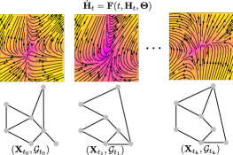
Figure 1: Graph neural ordinary differential equations (GDEs) model vector fields defined on graphs, both in cases when the structure is fixed or changes in time, via a continuum of graph neural network (GNN) layers.

GNNs have shown remarkable results in various application areas such as node classification (Zhuang and Ma, 2018; Gallicchio and Micheli, 2019), graph classification (Yan et al., 2018) and forecasting (Li et al., 2017; Wu et al., 2019) as well as generative tasks (Li et al., 2018b; You et al., 2018). A different but equally important class of inductive biases is concerned with the type of temporal behavior of the systems from which the data is collected i.e., discrete or continuous dynamics. Although deep learning has traditionally been a field dominated by discrete models, recent advances propose a treatment of neural networks equipped with a continuum of layers (Haber and Ruthotto, 2017; Chen et al., 2018). This view allows a reformulation of the forward and backward pass as the solution of the initial value problem of an ordinary differential equation (ODE). Such approaches allow direct modeling of ODEs and can guide discovery of novel general purpose deep learning models.

Blending graphs and differential equations

In this work we propose the system–theoretic framework of graph neural ordinary differential equations (GDEs) by defining ODEs parametrized by GNNs. GDEs are designed to inherit the ability to impose relational inductive biases of GNNs while retaining the dynamical system perspective of continuous–depth models. We validate GDEs experimentally on a static semi–supervised node classification task as well as spatio–temporal forecasting tasks. GDEs are shown to outperform their discrete GNN analogues: the different sources of performance improvement are identified and analyzed separately for static and dynamic settings.

Sequences of graphs

We extend the GDE framework to the spatio–temporal setting and formalize a general autoregressive GDE model as a hybrid dynamical system. The structure–dependent vector field learned by GDEs offers a data–driven approach to the modeling of dynamical networked systems (Lu and Chen, 2005; Andreasson et al., 2014), particularly when the governing equations are highly nonlinear and therefore challenging to approach with analytical methods. Autoregressive GDEs can adapt the prediction horizon by adjusting the integration interval of the ODE, allowing the model to track the evolution of the underlying system from irregular observations.

GDEs as general–purpose models

In general, no assumptions on the continuous nature of the data generating process are necessary in order for GDEs to be effective. Indeed, following recent work connecting different discretization schemes of ODEs (Lu et al., 2017) to previously known architectures such as FractalNets (Larsson et al., 2016), we show that GDEs can equivalently be utilized as high–performance general purpose models. In this setting, GDEs offer a grounded approach to the embedding of classic numerical schemes inside the forward pass of GNNs.

2 Graph Neural Ordinary Differential Equations

We begin by introducing the general formulation of GDEs.

2.1 General Framework

Definition of GDE

Without any loss of generality, the inter–layer dynamics of a GNN node feature matrix can be represented in the form:

$$\left\{\begin{matrix}[l]\mathbf{H}{(s+1)}=\mathbf{H}(s)+\mathbf{F}_{\operatorname{\mathcal{G}}}\left(s,\mathbf{H}(s),\bm{\Theta}(s)\right)\\ \mathbf{H}(0)=\mathbf{X}_{e}\end{matrix}\right.,~{}~{}s\in\operatorname{\mathbb{N}},$$

where $\mathbf{X}_{e}\in\operatorname{\mathbb{R}}^{n\times h}$ is an embedding of $\mathbf{X}$, $\mathbf{F}_{\operatorname{\mathcal{G}}}$ is a matrix–valued nonlinear function conditioned on graph $\mathcal{G}$ and $\bm{\Theta}(s)\in\operatorname{\mathbb{R}}^{p}$ is the tensor of trainable parameters of the $s$-th layer. Note that the explicit dependence on $s$ of the dynamics is justified in some graph architectures, such as diffusion graph convolutions (Atwood and Towsley, 2016). A graph neural differential ordinary equation (GDE) is defined as the following Cauchy problem:

$$\left\{\begin{matrix}[l]\dot{\mathbf{H}}(s)=\mathbf{F}_{\operatorname{\mathcal{G}}}\left(s,\mathbf{H}(s),\bm{\Theta}\right)\\ \mathbf{H}(0)=\mathbf{X}_{e}\end{matrix}\right.,~{}~{}s\in\operatorname{\mathcal{S}}\subset\operatorname{\mathbb{R}},$$ (1)

where $\mathbf{F}_{\operatorname{\mathcal{G}}}:\operatorname{\mathcal{S}}\times\operatorname{\mathbb{R}}^{n\times h}\times\operatorname{\mathbb{R}}^{p}\rightarrow\operatorname{\mathbb{R}}^{n\times h}$ is a depth–varying vector field defined on graph $\mathcal{G}$.

To reduce stiffness of learned vector fields, alleviating the computational burden of adaptive ODE solvers, the node features can be augmented in several ways (Dupont et al., 2019; Massaroli et al., 2020) by concatenating additional dimensions or prepending input layers to the GDE.

Well–posedness

Let $\operatorname{\mathcal{S}}:=[0,1]$. Under mild conditions on $\mathbf{F}$, namely Lipsichitz continuity with respect to $\mathbf{H}$ and uniform continuity with respect to $s$, for each initial condition (GDE embedded input) $\mathbf{X}_{e}$, the ODE in (1) admits a unique solution $\mathbf{H}(s)$ defined in the whole $\operatorname{\mathcal{S}}$. Thus there is a mapping $\bm{\Psi}$ from $\operatorname{\mathbb{R}}^{n\times h}$ to the space of absolutely continuous functions $\operatorname{\mathcal{S}}\to\operatorname{\mathbb{R}}^{n\times h}$ such that $\mathbf{H}:=\bm{\Psi}(\mathbf{X}_{e})$ satisfies the ODE in (1). This implies the the output $\mathbf{Y}$ of the GDE satisfies

$$\mathbf{Y}=\bm{\Psi}(\mathbf{X}_{e})(1).$$

Symbolically, the output of the GDE is obtained by the following

$$\mathbf{Y}=\mathbf{X}_{e}+\int_{\operatorname{\mathcal{S}}}\mathbf{F}_{\operatorname{\mathcal{G}}}(\tau,\mathbf{H}(\tau),\bm{\Theta})d\tau.$$

Note that applying an output layer or network to $\mathbf{Y}$ before passing it to downstream applications is generally beneficial.

Integration domain

We restrict the integration interval to $\operatorname{\mathcal{S}}=[0,1]$, given that any other integration time can be considered a rescaled version of $\operatorname{\mathcal{S}}$. Following (Chen et al., 2018) we use the number of function evaluations (NFE) of the numerical solver utilized to solve (1) as a proxy for model depth. In applications where $\operatorname{\mathcal{S}}$ acquires a specific meaning (i.e forecasting with irregular timestamps) the integration domain can be appropriately tuned to evolve GDE dynamics between arrival times (Rubanova et al., 2019) without assumptions on the functional form of the underlying vector field, as is the case for example with exponential decay in GRU–D (Che et al., 2018).

GDE training

GDEs can be trained with a variety of methods. Standard backpropagation through the computational graph, adjoint sensitivity method (Pontryagin et al., 1962) for $\mathcal{O}(1)$ memory efficiency (Chen et al., 2018), or backpropagation through a relaxed spectral elements discretization (Quaglino et al., 2019). Numerical instability in the form of accumulating errors on the adjoint ODE during the backward pass of Neural ODEs has been observed in (Gholami et al., 2019). A proposed solution is a hybrid checkpointing–adjoint scheme commonly employed in scientific computing (Wang et al., 2009), where the adjoint trajectory is reset at predetermined points in order control the error dynamics.

3 Taxonomy of GDEs

In the following, we taxonomize GDEs models distinguishing them into static and spatio–temporal (autoregressive) variants.

3.1 Static Models

Graph convolution differential equations

Based on graph spectral theory (Shuman et al., 2013; Sandryhaila and Moura, 2013), the residual version of graph convolution network (GCN) (Kipf and Welling, 2016) layers are in the form:

$$\mathbf{H}{(s+1)}=\mathbf{H}(s)+\sigma\left(\mathbf{L}_{\operatorname{\mathcal{G}}}\mathbf{H}(s)\bm{\Theta}(s)\right)$$ (2)

where $\mathbf{L}_{\operatorname{\mathcal{G}}}\in\operatorname{\mathbb{R}}^{n\times n}$ is the graph Laplacian and $\sigma$ is as nonlinear activation function. We denote with $\operatorname{\mathcal{C}}_{\operatorname{\mathcal{G}}}$ the graph convolution operator, i.e. $\operatorname{\mathcal{C}}_{\operatorname{\mathcal{G}}}\mathbf{H}(s)=\mathbf{L}_{\operatorname{\mathcal{G}}}\mathbf{H}(s)\bm{\Theta}(s)$. A general formulation of the continuous counterpart of GCNs, graph convolution differential equation (GCDE), is therefore obtained by defining $\mathbf{F}_{\operatorname{\mathcal{G}}}$ as a multilayer convolution, i.e.

$$\dot{\mathbf{H}}{(s)}=\mathbf{F}_{\tt GCN}(\mathbf{H}(s),\bm{\Theta}):=\operatorname{\mathcal{C}}^{N}_{\operatorname{\mathcal{G}}}\circ~{}\sigma\circ\operatorname{\mathcal{C}}^{N-1}_{\operatorname{\mathcal{G}}}\circ\cdots\circ\sigma\circ\operatorname{\mathcal{C}}^{1}_{\operatorname{\mathcal{G}}}\mathbf{H}(s)$$ (3)

Note that the Laplacian $\mathbf{L}_{\operatorname{\mathcal{G}}}$ can be computed in different ways, see e.g. (Bruna et al., 2013; Defferrard et al., 2016; Levie et al., 2018; Zhuang and Ma, 2018). Diffusion–type convolution layers (Li et al., 2017) are also compatible with the continuous–depth formulation.

Additional models and considerations

We include additional derivation of continuous counterparts of common static GNN models such as graph attention networks (GAT) (Veličković et al., 2017) and general message passing GNNs as supplementary material.

3.2 Spatio–Temporal Models

For settings involving a temporal component (i.e., modeling dynamical systems), the depth domain of GDEs coincides with the time domain $s\equiv t$ and can be adapted depending on the requirements. For example, given a time window $\Delta t$, the prediction performed by a GDE assumes the form:

$$\mathbf{H}{(t+\Delta t)}=\mathbf{H}(t)+\int_{t}^{t+\Delta t}\mathbf{F}\left(\tau,\mathbf{H}(\tau),\bm{\Theta}\right)d\tau,$$

regardless of the specific GDE architecture employed. Here, GDEs represent a natural model class for autoregressive modeling of sequences of graphs $\{\operatorname{\mathcal{G}}_{t}\}$ and seamlessly link to dynamical network theory. This line of reasoning naturally leads to an extension of classical spatio–temporal architectures in the form of hybrid dynamical systems (Van Der Schaft and Schumacher, 2000; Goebel et al., 2009), i.e., systems characterized by interacting continuous and discrete–time dynamics. Let $(\operatorname{\mathcal{K}},>)$, $(\operatorname{\mathcal{T}},>)$ be linearly ordered sets; namely, $\operatorname{\mathcal{K}}\subset\operatorname{\mathbb{N}}\setminus\{0\}$ and $\operatorname{\mathcal{T}}$ is a set of time instants, $\operatorname{\mathcal{T}}:=\{t_{k}\}_{k\in\operatorname{\mathcal{K}}}$. We suppose to be given a state–graph data stream which is a sequence in the form $\left\{\left(\mathbf{X}_{t},\operatorname{\mathcal{G}}_{t}\right)\right\}_{t\in\operatorname{\mathcal{T}}}$. Let us also define a hybrid time domain as the set $\operatorname{\mathcal{I}}:=\bigcup_{k\in\operatorname{\mathcal{K}}}\left([t_{k},t_{k+1}],k\right)$ and a hybrid arc on $\operatorname{\mathcal{I}}$ as a function $\bm{\Phi}$ such that for each $k\in\operatorname{\mathcal{K}}$, $t\mapsto\bm{\Phi}(t,k)$ is absolutely continuous in $\{t:(t,j)\in\operatorname{dom}\bm{\Phi}\}$. Our aim is to build a continuous model predicting, at each $t_{k}\in\operatorname{\mathcal{T}}$, the value of $\mathbf{X}_{t_{k+1}}$, given $\left(\mathbf{X}_{t},\operatorname{\mathcal{G}}_{t}\right)$. The core idea is to have a GDE smoothly steering the latent node features between two time instants and then apply some discrete operator, resulting in a “jump” of $\mathbf{H}$ which is then processed by an output layer. Solutions of the proposed continuous spatio–temporal model are therefore hybrid arcs.

Figure 2: Schematic of autoregressive GDEs as hybrid automata.

Autoregressive GDEs

The solution of a general autoregressive GDE model can be symbolically represented by:

$$\left\{\begin{matrix}[l]\dot{\mathbf{H}}({s})&=\mathbf{F}_{\operatorname{\mathcal{G}}_{t_{k}}}(\mathbf{H}(s),\bm{\Theta})&s\in[t_{k-1},t_{k}]\\[3.0pt] \mathbf{H}^{+}(s)&=\mathbf{G}_{\operatorname{\mathcal{G}}_{t_{k}}}(\mathbf{H}(s),\mathbf{X}_{t_{k}})&s=t_{k}\\[3.0pt] \mathbf{Y}&=\mathbf{K}(\mathbf{H}(s))&s=t_{k}\end{matrix}\right.k\in\operatorname{\mathcal{K}},$$ (4)

where $\mathbf{F},\mathbf{G},\mathbf{K}$ are GNN–like operators or general neural network layers and $\mathbf{H}^{+}$ represents the value of $\mathbf{H}$ after the discrete transition. The evolution of system (4) is indeed a sequence of hybrid arcs defined on a hybrid time domain. A graphical representation of the overall system is given by the hybrid automata as shown in Fig. 2. Compared to standard recurrent models which are only equipped with discrete jumps, system (4) incorporates a continuous flow of latent node features $\mathbf{H}$ between jumps. This feature of autoregressive GDEs allows them to track the evolution of dynamical systems from observations with irregular time steps. In the experiments we consider $\mathbf{G}$ to be a GRU cell (Cho et al., 2014), obtaining graph convolutional differential equation–GRU (GCDE–GRU). Alternatives such as GCDE–RNNs or GCDE–LSTMs can be similarly obtained by replacing $\mathbf{G}$ with other common recurrent modules, such as vanilla RNNs or LSTMs (Hochreiter and Schmidhuber, 1997). It should be noted that the operators $\mathbf{F},\mathbf{G},\mathbf{K}$ can themselves have multi–layer structure.

4 Experiments

We evaluate GDEs on a suite of different tasks. The experiments and their primary objectives are summarized below:

• Semi–supervised node classification on static, standard benchmark datasets Cora, Citeseer, Pubmed (Sen et al., 2008). We investigate the usefulness of the proposed method in a static setting via an ablation analysis that directly compares GCNs and analogue GCDEs solved with fixed–step and adaptive solvers.

• Trajectory extrapolation task on a synthetic multi–agent dynamical system. We compare Neural ODEs and GDEs, providing a motivating example for the introduction of additional biases in the form of second–order models (Yıldız et al., 2019; Massaroli et al., 2020).

• Traffic forecasting on an undersampled version of PeMS (Yu et al., 2018) dataset. We measure the performance improvement obtained by a correct inductive bias on continuous dynamics and robustness to irregular timestamps.

The code will be open–sourced after the review phase and is included in the submission.

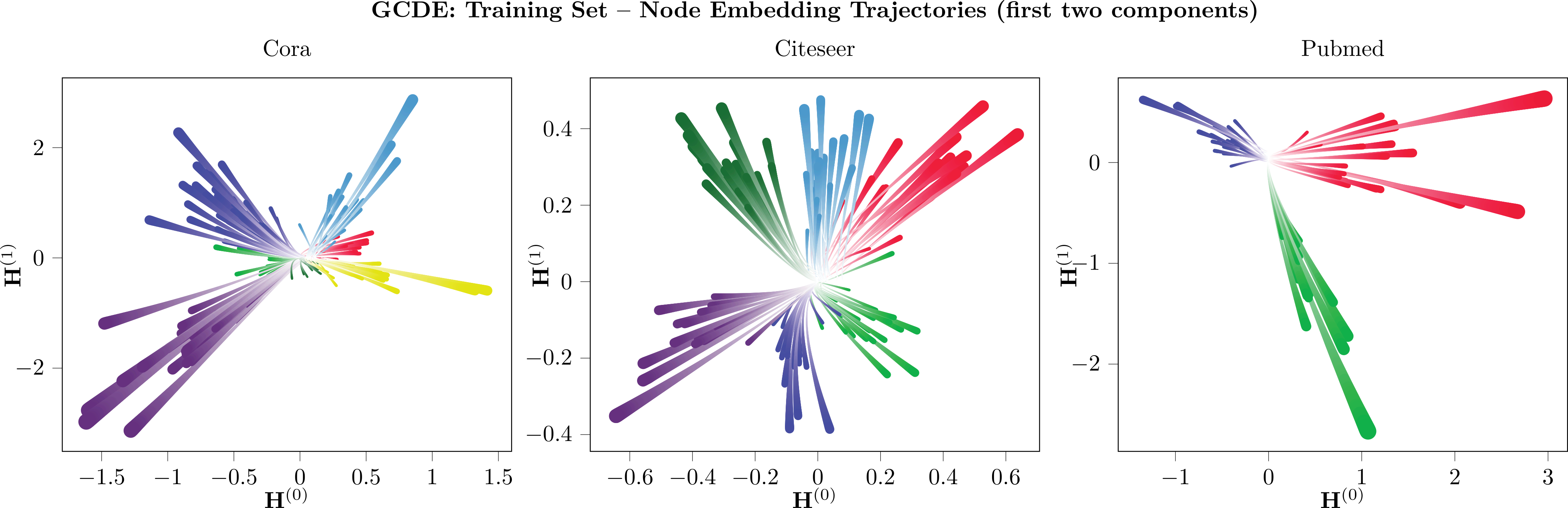
Figure 3: Node embedding trajectories defined by a forward pass of GCDE–dpr5 on Cora, Citeseer and Pubmed. Color differentiates between node classes.

Model (NFE)	Cora	Citeseer	Pubmed
GCN	$81.4\pm 0.5\%$	$70.9\pm 0.5\%$	$79.0\pm 0.3\%$
GCN∗	$82.8\pm 0.3\%$	$71.2\pm 0.4\%$	$79.5\pm 0.4\%$
GCDE–rk2 (2)	$83.0\pm 0.6\%$	$72.3\pm 0.5\%$	$\textbf{79.9}\pm 0.3\%$
GCDE–rk4 (4)	$\textbf{83.8}\pm 0.5\%$	$\textbf{72.5}\pm 0.5\%$	$79.5\pm 0.4\%$
GCDE–dpr5 (158)	$81.8\pm 1.2\%$	$68.3\pm 1.2\%$	$78.5\pm 0.7\%$

Table 1: Test results across 100 runs ($\mu$ and $\sigma$). All models have hidden dimension $64$.

4.1 Transductive Node Classification

Experimental setup

The first task involves performing semi–supervised node classification on static graphs collected from baseline datasets Cora, Pubmed and Citeseer (Sen et al., 2008). Main goal of these experiments is to perform an ablation study on the source of possible performance advantages of the GDE framework in settings that do not involve continuous dynamical systems. The $L_{2}$ weight penalty is set to $5\cdot 10^{-4}$ on Cora, Citeseer and $10^{-3}$ on Pubmed as a strong regularizer due to the small size of the training set (Monti et al., 2017). We report mean and standard deviation across $100$ training runs. Since our experimental setup follows (Kipf and Welling, 2016) to allow for a fair comparison, other baselines present in recent GNN literature can be directly compared with Table 1.

Models and baselines

All convolution–based models are equipped with a latent dimension of $64$. We include results for best performing vanilla GCN baseline presented in (Veličković et al., 2017). To avoid flawed comparisons, we further evaluate an optimized version of GCN, GCN^∗, sharing exact architecture, as well as training and validation hyperparameters with the GCDE models. We experimented with different number of layers for GCN^∗: (2, 3, 4, 5, 6) and select $2$, since it achieves the best results. The performance of graph convolution differential equation (GCDE) is assessed with both a fixed-step solver Runge–Kutta (Runge, 1895; Kutta, 1901) as well as an adaptive–step solver, Dormand–Prince (Dormand and Prince, 1980). The resulting models are denoted as GCDE–rk4 and GCDE–dpr5, respectively. We utilize the torchdiffeq (Chen et al., 2018) PyTorch package to solve and backpropagate through the ODE solver.

Continuous–depth models in static tasks

Ensuring a low error solution to the ODE parametrized by the model with adaptive–step solvers does not offer particular advantages in image classification tasks (Chen et al., 2018) compared to equivalent discrete models. While there is no reason to expect performance improvements solely from the transition away from discrete architectures, continuous–depth allows for the embedding of numerical ODE solvers in the forward pass. Multi–step architectures have previously been linked to ODE solver schemes (Lu et al., 2017) and routinely outperform their single–step counterparts (Larsson et al., 2016; Lu et al., 2017). We investigate the performance gains by employing the GDE framework in static settings as a straightforward approach to the embedding of numerical ODE solvers in GNNs.

Results

The variants of GCDEs solved with fixed–step schemes are shown to outperform or match GCN^∗ across all datasets, with the margin of improvement being highest on Cora and Citeseer. Introducing GCDE–rk2 and GCDE–rk4 is observed to provide the most significant accuracy increases in more densely connected graphs or with larger training sets. In particular, GCDE–rk4 outperforming GCDE–rk2 indicates that, given equivalent network architectures, higher order ODE solvers are generally more effective, provided the graph is dense enough to benefit from the additional computation. Additionally, training GCDEs with adaptive step solvers naturally leads to deeper models than possible with vanilla GCNs, whose layer depth greatly reduces performance. However, the high number of function evaluation (NFEs) of GCDE–dpr5 necessary to stay within the ODE solver tolerances causes the model to overfit and therefore generalize poorly. We visualize the first two components of GCDE–dpr5 node embedding trajectories in Figure 3. The trajectories are divergent, suggesting a non–decreasing classification performance for GCDE models trained with longer integration times. We provide complete visualization of accuracy curves in Appendix C.

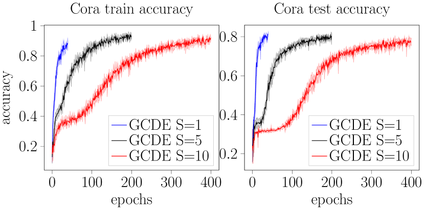
Figure 4: Cora accuracy of GCDE models with different integration times $s$.

Resilience to integration time

For each integration time $S\in[1,5,10]$, we train $100$ GCDE-dpr5 models on Cora and report average metrics, along with $1$ standard deviation confidence intervals in Figure 4. GCDEs are shown to be resilient to changes in $S$; however, GCDEs with longer integration times require more training epochs to achieve comparable accuracy. This result suggests that, indeed, GDEs are immune to node oversmoothing (Oono and Suzuki, 2019).

4.2 Multi–Agent Trajectory Extrapolation

Experimental setup

We evaluate GDEs and a collection of deep learning baselines on the task of extrapolating the dynamical behavior of a synthetic mechanical multi–particle system. Particles interact within a certain radius with a viscoelastic force. Outside the mutual interactions, captured by a time–varying adjacency matrix $\mathbf{A}_{t}$, the particles would follow a periodic motion. The adjaciency matrix $\mathbf{A}_{t}$ is computed along the trajectory as:

$$\mathbf{A}_{t}^{(ij)}=\left\{\begin{matrix}[l]1&2\|\mathbf{x}_{i}(t)-\mathbf{x}_{j}(t)\|\leq r\\ 0&\text{otherwise}\end{matrix}\right.~{},$$

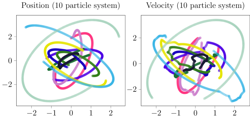
Figure 5: Example position and velocity trajectories of the multi–particle system.

where $\mathbf{x}_{i}(t)$ is the position of node $i$ at time $t$. Therefore, $\mathbf{A}_{t}$ results to be symmetric, $\mathbf{A}_{t}=\mathbf{A}_{t}^{\top}$ and yields an undirected graph. The dataset is collected by integrating the system for $T=5s$ with a fixed step–size of $dt=1.95\cdot 10^{-3}$ and is split evenly into a training and test set. We consider $10$ particle systems. An example trajectory is shown in Figure 5. All models are optimized to minimize mean–squared–error (MSE) of 1–step predictions using Adam (Kingma and Ba, 2014) with constant learning rate $0.01$. We measure test mean average percentage error (MAPE) of model predictions in different extrapolation settings. Extrapolation steps denotes the number of predictions each model $\Phi$ has to perform without access to the nominal trajectory. This is achieved by recursively letting inputs at time $t$ be model predictions at time $t-\Delta t$ i.e $\hat{\mathbf{Y}}_{t+\Delta t}=\phi(\hat{\mathbf{Y}}_{t})$ for a certain number of extrapolation steps, after which the model is fed the actual nominal state $\mathbf{X}$ and the cycle is repeated until the end of the test trajectory. For a robust comparison, we report mean and standard deviation across 10 seeded training and evaluation runs. Additional experimental details, including the analytical formulation of the dynamical system, are provided as supplementary material.

Models and baselines

As the vector field depends only on the state of the system, available in full during training, the baselines do not include recurrent modules. We consider the following models:

• A 3–layer fully-connected neural network, referred to as Static. No assumption on the dynamics

• A vanilla Neural ODE with the vector field parametrized by the same architecture as Static. ODE assumption on the dynamics.

• A 3–layer convolution GDE, GCDE. Dynamics assumed to be determined by a blend of graphs and ODEs

• A 3–layer, second–order (Yıldız et al., 2019; Massaroli et al., 2020) GCDE and referred to as GCDE-II. GCDE assumptions in addition to second–order ODE dynamics.

A grid hyperparameter search on number of layers, ODE solver tolerances and learning rate is performed to optimize Static and Neural ODEs. We use the same hyperparameters for GDEs.

Figure 6: Test extrapolation MAPE averaged across 10 experiments. Shaded area and error bars indicate 1–standard deviation intervals.

Results

Figure 6 shows the growth rate of test MAPE error as the number of extrapolation steps is increased. Static fails to extrapolate beyond the 1–step setting seen during training. Neural ODEs overfit spurious particle interaction terms and their error rapidly grows as the number of extrapolation steps is increased. GCDEs, on the other hand, are able to effectively leverage relational information to track the system: we provide complete visualization of extrapolation trajectory comparisons in the supplementary material. Lastly, GCDE-IIs outperform first–order GCDEs as their structure inherently possesses crucial information about the relative relationship of positions and velocities that is accurate with respect to the observed dynamical system.

4.3 Traffic Forecasting

Experimental setup

We evaluate the effectiveness of autoregressive GDE models on forecasting tasks by performing a series of experiments on the established PeMS traffic dataset. We follow the setup of (Yu et al., 2018) in which a subsampled version of PeMS, PeMS7(M), is obtained via selection of 228 sensor stations and aggregation of their historical speed data into regular 5 minute frequency time series. We construct the adjacency matrix $\mathbf{A}$ by thresholding of the Euclidean distance between observation stations i.e. when two stations are closer than the threshold distance, an edge between them is included. The threshold is set to the 40${}^{\text{th}}$ percentile of the station distances distribution. To simulate a challenging environment with missing data and irregular timestamps, we undersample the time series by performing independent Bernoulli trials on each data point. Results for 3 increasingly challenging experimental setups are provided: undersampling with $30\%$, $50\%$ and $70\%$ of removal. In order to provide a robust evaluation of model performance in regimes with irregular data, the testing is repeated $20$ times per model, each with a different undersampled version of the test dataset. We collect root mean square error (RMSE) and MAPE. More details about the chosen metrics and data are included as supplementary material.

Models and baselines

In order to measure performance gains obtained by GDEs in settings with data generated by continuous time systems, we employ a GCDE–GRU–dopri5 as well as its discrete counterpart GCGRU (Zhao et al., 2018). To contextualize the effectiveness of introducing graph representations, we include the performance of GRUs since they do not directly utilize structural information of the system in predicting outputs. Apart from GCDE–GRU, both baseline models have no innate mechanism for handling timestamp information. For a fair comparison, we include timestamp differences between consecutive samples and sine–encoded (Petneházi, 2019) absolute time information as additional features. All models receive an input sequence of $5$ graphs to perform the prediction.

Model	MAPE30%	RMSE30%	MAPE50%	RMSE50%	MAPE70%	RMSE70%	MAPE100%	RMSE100%
GRU	$27.14\pm 0.45$	$13.25\pm 0.11$	$27.08\pm 0.26$	$13.22\pm 0.07$	$27.24\pm 0.19$	$13.28\pm 0.05$	$27.20$	$13.29$
GCGRU	$23.60\pm 0.38$	$11.97\pm 0.03$	$22.86\pm 0.22$	$11.78\pm 0.06$	$21.33\pm 0.16$	$11.20\pm 0.04$	$20.92$	$10.87$
GCDE-GRU	$\mathbf{22.95}\pm 0.37$	$\mathbf{11.67}\pm 0.10$	$\mathbf{21.25}\pm 0.21$	$\mathbf{11.04}\pm 0.05$	$\mathbf{20.94}\pm 0.14$	$\mathbf{10.95}\pm 0.04$	$\mathbf{20.46}$	$\mathbf{10.766}$

Table 2: Forecasting test results across 20 runs (mean and standard deviation). MAPE_i indicates $i\%$ undersampling of the test set.

Results

Non–constant differences between timestamps result in a challenging forecasting task for a single model since the average prediction horizon changes drastically over the course of training and testing. Traffic systems are intrinsically dynamic and continuous in nature and, therefore, a model able to track continuous underlying dynamics is expected to offer improved performance. Since GCDE-GRUs and GCGRUs are designed to match in structure we can measure this performance increase from the results shown in Table 2. GCDE–GRUs outperform GCGRUs and GRUs in all undersampling regimes. Additional details and prediction visualizations are included in Appendix C.

5 Related work

There exists a concurrent line of work (Xhonneux et al., 2019) introducing a GNN variant evaluated on static node classification tasks where the output is the analytical solution of a linear ODE. Sanchez-Gonzalez et al. (2019) proposes using graph networks (GNs) (Battaglia et al., 2018) and ODEs to track Hamiltonian functions, whereas (Deng et al., 2019) introduces a GNN version of continuous normalizing flows (Chen et al., 2018; Grathwohl et al., 2018) for generative modeling, extending (Liu et al., 2019). Our goal is developing a unified system–theoretic framework for continuous–depth GNNs covering the main variants of static and spatio–temporal GNN models. Our work provides extensive experimental evaluations on both static as well as dynamic tasks with the primary aim of uncovering the sources of performance improvement of GDEs in each setting.

6 Discussion

Unknown or dynamic topology

Several lines of work concerned with learning the graph structure directly from data exist, either by inferring the adjacency matrix within a probabilistic framework (Kipf et al., 2018) or using a soft–attention (Vaswani et al., 2017) mechanism (Choi et al., 2017; Li et al., 2018a; Wu et al., 2019). In particular, the latter represents a commonly employed approach to the estimation of a dynamic adjacency matrix in spatio–temporal settings. Due to the algebraic nature of the relation between the attention operator and the node features, GDEs are compatible with its use inside the GNN layers parametrizing the vector field. Thus, if an optimal adaptive graph representation $\mathbf{S}(s,\mathbf{H})$ is computed through some attentive mechanism, standard convolution GDEs can be replaced by $\dot{\mathbf{H}}=\sigma\left(\mathbf{S}\mathbf{H}\bm{\Theta}\right).$

Addition or removal of nodes

GDE variants operating on sequences of dynamically changing graphs can, without changes to the formulation, directly accommodate addition or removal of nodes as long as its number remains constant during the flows. In fact, the size of parameter matrix $\bm{\Theta}$ exclusively depends on the node feature dimension, resulting in resilience to a varying number of nodes.

7 Conclusion

In this work we introduce graph neural ordinary differential equations (GDE), the continuous–depth counterpart to graph neural networks (GNN) where the inputs are propagated through a continuum of GNN layers. The GDE formulation is general, as it can be adapted to include many static and autoregressive GNN models. GDEs are designed to offer a data–driven modeling approach for dynamical networks, whose dynamics are defined by a blend of discrete topological structures and differential equations. In sequential forecasting problems, GDEs can accommodate irregular timestamps and track the underlying continuous dynamics, whereas in static settings they offer computational advantages by allowing for the embedding of black–box numerical solvers in their forward pass. GDEs have been evaluated on both static and dynamic tasks and have been shown to outperform their discrete counterparts.

 

Graph Neural Ordinary Differential Equations
Supplementary Material

 

Appendix A Graph Neural Ordinary Differential Equations

Notation

Let $\operatorname{\mathbb{N}}$ be the set of natural numbers and $\operatorname{\mathbb{R}}$ the set of reals. Scalars are indicated as lowercase letters, vectors as bold lowercase, matrices and tensors as bold uppercase and sets with calligraphic letters. Indices of arrays and matrices are reported as superscripts in round brackets.

Let $\operatorname{\mathcal{V}}$ be a finite set with $|\operatorname{\mathcal{V}}|=n$ whose element are called nodes and let $\operatorname{\mathcal{E}}$ be a finite set of tuples of $\operatorname{\mathcal{V}}$ elements. Its elements are called edges and are such that $\forall e_{ij}\in\operatorname{\mathcal{E}},~{}e_{ij}=(v_{i},v_{j})$ and $v_{i},v_{j}\in\operatorname{\mathcal{V}}$. A graph $\operatorname{\mathcal{G}}$ is defined as the collection of nodes and edges, i.e. $\operatorname{\mathcal{G}}:=(\operatorname{\mathcal{V}},\operatorname{\mathcal{E}})$. The adjeciency matrix $\mathbf{A}\in\operatorname{\mathbb{R}}^{n\times n}$ of a graph is defined as

$$\mathbf{A}^{(ij)}=\left\{\begin{matrix}[l]1&e_{ij}\in\operatorname{\mathcal{E}}\\ 0&e_{ij}\not\in\operatorname{\mathcal{E}}\end{matrix}\right.~{}.$$

If $\operatorname{\mathcal{G}}$ is an attributed graph, the feature vector of each $v\in\operatorname{\mathcal{V}}$ is $\mathbf{x}_{v}\in\operatorname{\mathbb{R}}^{n_{x}}$. All the feature vectors are collected in a matrix $\mathbf{X}\in\operatorname{\mathbb{R}}^{n\times n_{x}}$. Note that often, the features of graphs exhibit temporal dependency, i.e. $\mathbf{X}:=\mathbf{X}_{t}$.

A.1 General Static Formulation

For clarity and as an easily accessible reference, we include below a general formulation table for the static case

Note that the general formulation provided in (4) can similarly serve as a reference for the spatio–temporal case.

A.2 Computational Overhead

As is the case for other models sharing the continuous–depth formulation (Chen et al., 2018), the computational overhead required by GDEs depends mainly by the numerical methods utilized to solve the differential equations. We can define two general cases for fixed–step and adaptive–step solvers.

Fixed–step

In the case of fixed–step solvers of k–th order e.g Runge–Kutta–k (Runge, 1895), the time complexity is $O(nk)$ where $n:=S/\epsilon$ defines the number of steps necessary to cover $[0,S]$ in fixed–steps of $\epsilon$.

Adaptive–step

For general adaptive–step solvers, computational overhead ultimately depends on the error tolerances. While worst–case computation is not bounded (Dormand and Prince, 1980), a maximum number of steps can usually be set algorithmically.

A.3 Additional GDEs

Message passing GDEs

Let us consider a single node $v\in\operatorname{\mathcal{V}}$ and define the set of neighbors of $v$ as $\operatorname{\mathcal{N}}(v):=\{u\in\operatorname{\mathcal{V}}~{}:~{}(v,u)\in\operatorname{\mathcal{E}}\lor(u,v)\in\operatorname{\mathcal{E}}\}$. Message passing neural networks (MPNNs) perform a spatial–based convolution on the node $v$ as

$$\mathbf{h}^{(v)}{(s+1)}=\mathbf{u}\left[\mathbf{h}^{(v)}(s),\sum_{u\in\operatorname{\mathcal{N}}(v)}\mathbf{m}\left({\mathbf{h}^{(v)}(s),\mathbf{h}^{(u)}(s)}\right)\right],$$ (5)

where, in general, $\mathbf{h}^{v}(0)=\mathbf{x}_{v}$ while $\mathbf{u}$ and $\mathbf{m}$ are functions with trainable parameters. For clarity of exposition, let $\mathbf{u}(\mathbf{x},\mathbf{y}):=\mathbf{x}+\mathbf{g}(\mathbf{y})$ where $\mathbf{g}$ is the actual parametrized function. The (5) becomes

$$\mathbf{h}^{(v)}{(s+1)}=\mathbf{h}^{(v)}(s)+\mathbf{g}\left[\sum_{u\in\operatorname{\mathcal{N}}(v)}\mathbf{m}\left({\mathbf{h}^{(v)}(s),\mathbf{h}^{(u)}(s)}\right)\right],$$ (6)

and its continuous–depth counterpart, graph message passing differential equation (GMDE) is:

$$\dot{\mathbf{h}}^{(v)}{(s)}=\mathbf{f}^{(v)}_{\tt MPNN}(\mathbf{H},\bm{\Theta}):=\mathbf{g}\left[\sum_{u\in\operatorname{\mathcal{N}}(v)}\mathbf{m}\left({\mathbf{h}^{(v)}(s),\mathbf{h}^{(u)}}(s)\right)\right].$$

Attention GDEs

Graph attention networks (GATs) (Veličković et al., 2017) perform convolution on the node $v$ as

$$\mathbf{h}^{(v)}{(s+1)}=\sigma\left(\sum_{u\in\operatorname{\mathcal{N}}(v)\cup v}{\alpha_{vu}\bm{\Theta}(s)\mathbf{h}^{(u)}}(s)\right).$$ (7)

Similarly, to GCNs, a virtual skip connection can be introduced allowing us to define the graph attention differential equation (GADE):

$$\dot{\mathbf{h}}^{(v)}{(s)}=\mathbf{f}^{(v)}_{\tt GAT}(\mathbf{H},\bm{\Theta}):=\sigma\left(\sum_{u\in\operatorname{\mathcal{N}}(v)\cup v}{\alpha_{vu}\bm{\Theta}\mathbf{h}^{(u)}}(s)\right),$$

where $\alpha_{vu}$ are attention coefficient which can be computed following (Veličković et al., 2017).

Appendix B Spatio–Temporal GDEs

We include a complete description of GCGRUs to clarify the model used in our experiments.

Figure 7: Test accuracy curves on Cora and Citeseer (100 experiments). Shaded area indicates the 1 standard deviation interval.

B.1 GCGRU Cell

Following GCGRUs (Zhao et al., 2018), we perform an instantaneous jump of $\mathbf{H}$ at each time $t_{k}$ using the next input features $\mathbf{X}_{t_{k}}$. Let $\mathbf{L}_{\operatorname{\mathcal{G}}_{t_{k}}}$ be the graph Laplacian of graph $\operatorname{\mathcal{G}}_{t_{k}}$, which can computed in several ways (Bruna et al., 2013; Defferrard et al., 2016; Levie et al., 2018; Zhuang and Ma, 2018). Then, let

$$\mathbf{Z} :=\sigma\left(\mathbf{L}_{\operatorname{\mathcal{G}}_{t_{k}}}\mathbf{X}_{t_{k}}\bm{\Theta}_{xz}+\mathbf{L}_{\operatorname{\mathcal{G}}_{t_{k}}}\mathbf{H}\bm{\Theta}_{hz}\right),$$ (8)

$$\mathbf{R} :=\sigma\left(\mathbf{L}_{\operatorname{\mathcal{G}}_{t_{k}}}\mathbf{X}_{t_{k}}\bm{\Theta}_{xr}+\mathbf{L}_{\operatorname{\mathcal{G}}_{t_{k}}}\mathbf{H}\bm{\Theta}_{hr}\right),$$

$$\tilde{\mathbf{H}} :=\tanh\left(\mathbf{L}_{\operatorname{\mathcal{G}}_{t_{k}}}\mathbf{X}_{t_{k}}\bm{\Theta}_{xh}+\mathbf{L}_{\operatorname{\mathcal{G}}_{t_{k}}}\left(\mathbf{R}\odot\mathbf{H}\right)\bm{\Theta}_{hh}\right).$$

Finally, the post–jump node features are obtained as

$$\mathbf{H}^{+} ={\tt GCGRU}(\mathbf{H},\mathbf{X}_{t}):=\mathbf{Z}\odot\mathbf{H}+(\mathbb{1}-\mathbf{Z}),\odot\tilde{\mathbf{H}}$$ (9)

where $\bm{\Theta}_{xz},~{}\bm{\Theta}_{hz},~{}\bm{\Theta}_{xr},~{}\bm{\Theta}_{hr},~{}\bm{\Theta}_{xh},~{}\bm{\Theta}_{hh}$ are matrices of trainable parameters, $\sigma$ is the standard sigmoid activation and $\mathbb{1}$ is all–ones matrix of suitable dimensions.

Appendix C Additional experimental details

Computational resources

We carried out all experiments on a cluster of 4x12GB NVIDIA^® Titan Xp GPUs and CUDA 10.1. The models were trained on GPU.

C.1 Node Classification

Training hyperparameters

All models are trained for $2000$ epochs using Adam (Kingma and Ba, 2014) with learning rate $lr=10^{-3}$ on Cora, Citeseer and $lr=10^{-2}$ on Pubmed due to its training set size. The reported results are obtained by selecting the lowest validation loss model after convergence (i.e. in the epoch range $1000$ – $2000$). Test metrics are not utilized in any way during the experimental setup. For the experiments to test resilience to integration time changes, we set a higher learning rate for all models i.e. $lr=10^{-2}$ to reduce the number of epochs necessary to converge.

Architectural details

SoftPlus is used as activation for GDEs. Smooth activations have been observed to reduce stiffness (Chen et al., 2018) of the ODE and therefore the number of function evaluations (NFE) required for a solution that is within acceptable tolerances. All the other activation functions are rectified linear units (ReLU). The exact input and output dimensions for the GCDE architectures are reported in Table 3. The vector field $\mathbf{F}$ of GCDEs–rk2 and GCDEs–rk4 is parameterized by two GCN layers. GCDEs–dopri5 shares the same structure without GDE–2 (GCN). Input GCN layers are set to dropout $0.6$ whereas GCN layers parametrizing $\mathbf{F}$ are set to $0.9$.

Layer	Input dim.	Output dim.	Activation
GCN–in	dim. in	$64$	ReLU
GDE–1 (GCN)	$64$	$64$	Softplus
GDE–2 (GCN)	$64$	$64$	None
GCN-out	64	dim. out	None

Table 3: General architecture for GCDEs on node classification tasks. GCDEs applied to different datasets share the same architecture. The vector field $\mathbf{F}$ is parameterized by two GCN layers. GCDEs–dopri5 shares the same structure without GDE–2 (GCN).

Figure 8: Snapshots of the evolution of adjacency matrix $\mathbf{A}_{t}$ throughout the dynamics of the multi–particle system. Yellow indicates the presence of an edge and therefore a reciprocal force acting on the two bodies

C.2 Multi–Agent System Dynamics

Dataset

Let us consider a planar multi agent system with states $\mathbf{x}_{i}$ ($i=1,\dots,n$) and second–order dynamics:

$$\ddot{\mathbf{x}}_{i} =-\mathbf{x}_{i}-\sum_{j\in\operatorname{\mathcal{N}}_{i}}\mathbf{f}_{ij}(\mathbf{x}_{i},\mathbf{x}_{j},\dot{\mathbf{x}}_{i},\dot{\mathbf{x}}_{j}),$$

where

$$\mathbf{f}_{ij}=-\left[\alpha\left(\|\mathbf{x}_{i}-\mathbf{x}_{j}\|-r\right)+\beta\frac{\langle\dot{\mathbf{x}}_{i}-\dot{\mathbf{x}}_{j},\mathbf{x}_{i}-\mathbf{x}_{j}\rangle}{\|\mathbf{x}_{i}-\mathbf{x}_{j}\|}\right]\mathbf{n}_{ij},$$

$$\mathbf{n}_{ij}=\frac{\mathbf{x}_{i}-\mathbf{x}_{j}}{\|\mathbf{x}_{i}-\mathbf{x}_{j}\|},\quad\alpha,~{}\beta,~{}r>0,$$

and

$$\quad\operatorname{\mathcal{N}}_{i}:=\left\{j:2\|\mathbf{x}_{i}-\mathbf{x}_{j}\|\leq r\land j\not=i\right\}.$$

The force $\mathbf{f}_{ij}$ resembles the one of a spatial spring with drag interconnecting the two agents. The term $-\mathbf{x}_{i}$, is used instead to stabilize the trajectory and avoid the ”explosion” of the phase–space. Note that $\mathbf{f}_{ij}=-\mathbf{f}_{ji}$. The adjaciency matrix $\mathbf{A}_{t}$ is computed along a trajectory

$$\mathbf{A}_{t}^{(ij)}=\left\{\begin{matrix}[l]1&2\|\mathbf{x}_{i}(t)-\mathbf{x}_{j}(t)\|\leq r\\ 0&\text{otherwise}\end{matrix}\right.,$$

which indeed results to be symmetric, $\mathbf{A}_{t}=\mathbf{A}_{t}^{\top}$ and thus yields an undirected graph. Figure 8 visualizes an example trajectory of $\mathbf{A}_{t}$.

Model	MAPE1	MAPE3	MAPE5	MAPE10	MAPE15	MAPE20	MAPE50
Static	$26.12$	$160.56$	$197.20$	$235.21$	$261.56$	$275.60$	$360.39$
Neural ODE	$26.12$	$52.26$	$92.31$	$156.26$	$238.14$	$301.85$	$668.47$
GDE	$13.53$	$15.22$	$18.76$	$27.76$	$33.90$	$42.22$	$77.64$
GDE–II	$13.46$	$14.75$	$17.81$	$27.77$	$32.28$	$40.64$	$73.75$

Table 4: Mean MAPE results across the 10 multi–particle dynamical system experiments. MAPE_i indicates results for $i$ extrapolation steps on the full test trajectory.

Figure 9: Test extrapolation, $5$ steps. Trajectory predictions of Neural ODEs and GDEs. The extrapolation is terminated after 5 steps and the nominal state is fed to the model.

We collect a single rollout with $T=5$, $dt=1.95\cdot 10^{-3}$ and $n=10$. The particle radius is set to $r=1$.

Architectural details

Node feature vectors are $4$ dimensional, corresponding to the dimension of the state, i.e. position and velocity. Neural ODEs and Static share an architecture made up of 3 fully–connected layers: $4n$, $8n$, $8n$, $4n$ where $n=10$ is the number of nodes. The last layer is linear. We evaluated different hidden layer dimensions: $8n$, $16n$, $32n$ and found $8n$ to be the most effective. Similarly, the architecture of first order GCDEs is composed of 3 GCN layers: $4$, $16$, $16$, $4$. Second–order GCDEs, on the other hand, are augmented by $4$ dimensions: $8$, $32$, $32$, $8$. We experimented with different ways of encoding the adjacency matrix $\mathbf{A}$ information into Neural ODEs and $Static$ but found that in all cases it lead to worse performance.

Additional results

We report in Figure 9 test extrapolation predictions of $5$ steps for GDEs and the various baselines. Neural ODEs fail to track the system, particularly in regions of the state space where interaction forces strongly affect the dynamics. GDEs, on the other hand, closely track both positions and velocities of the particles.

C.3 Traffic Forecasting

Dataset and metrics

The timestamp differences between consecutive graphs in the sequence varies due to undersampling. The distribution of timestamp deltas (5 minute units) for the three different experiment setups (30%, 50%, 70% undersampling) is shown in Figure 11.

As a result, GRU takes 230 dimensional vector inputs (228 sensor observations + 2 additional features) at each sequence step. Both GCGRU and GCDE–GRU graph inputs with and 3 dimensional node features (observation + 2 additional feature). The additional time features are excluded for the loss computations. We include MAPE and RMSE test measurements, defined as follows:

Figure 10: Traffic data training results of 50% undersampling.

Figure 11: Distribution of deltas between timestamps $t_{k+1}-t_{k}$ in the undersampled dataset. The time scale of required predictions varies greatly during the task.

$$\text{MAPE}(\mathbf{y},\hat{\mathbf{y}})=\frac{100\%}{pT}\left\lVert\sum_{t=1}^{T}(\mathbf{y}_{t}-\hat{\mathbf{y}}_{t})\oslash\mathbf{y}_{t}\right\rVert_{1},$$ (10)

where $\mathbf{y},\text{and}\ \hat{\mathbf{y}}\in\mathbb R^{p}$ is the set of vectorized target and prediction of models respectively. $\oslash$ and $\left\lVert\cdot\right\rVert_{1}$ denotes Hadamard division and the 1-norm of vector.

$$\text{RMSE}(\mathbf{y},\hat{\mathbf{y}}) =\frac{1}{p}\left\lVert\sqrt{\frac{1}{T}\sum_{t=1}^{T}(\mathbf{y}_{t}-\hat{\mathbf{y}}_{t})^{2}}\right\rVert_{1},$$

where $(\cdot)^{2}$ and $\sqrt{\cdot}$ denotes the element-wise square and square root of the input vector, respectively. $\mathbf{y}_{t}\ \text{and}\ \hat{\mathbf{y}}_{t}$ denote the target and prediction vector.

Figure 12: Traffic data prediction results of 50% undersampling. GCDE–GRUs are able to evolve the latents between timestamps and provide a more accurate fit.

Architectural details

We employed two baseline models for contextualizing the importance of key components of GCDE–GRU. GRUs architectures are equipped with 1 GRU layer with hidden dimension 50 and a 2 layer fully–connected head to map latents to predictions. GCGRUs employ a GCGRU layer with 46 hidden dimension and a 2 layer fully–connected head. Lastly, GCDE–GRU shares the same architecture GCGRU with the addition of the flow $\mathbf{F}$ tasked with evolving the hidden features between arrival times. $\mathbf{F}$ is parametrized by 2 GCN layers, one with tanh activation and the second without activation. ReLU is used as the general activation function.

Training hyperparameters

All models are trained for 40 epochs using Adam(Kingma and Ba, 2014) with $lr=10^{-2}$. We schedule $lr$ by using cosine annealing method (Loshchilov and Hutter, 2016) with $T_{0}=10$. The optimization is carried out by minimizing the mean square error (MSE) loss between predictions and corresponding targets.

Additional results

Training curves of the models are presented in the Fig 10. All of models achieved nearly 13 in RMSE during training and fit the dataset. However, due to the lack of dedicated spatial modeling modules, GRUs were unable to generalize to the test set and resulted in a mean value prediction.

References

- Andreasson et al. (2014) M. Andreasson, D. V. Dimarogonas, H. Sandberg, and K. H. Johansson. Distributed control of networked dynamical systems: Static feedback, integral action and consensus. IEEE Transactions on Automatic Control, 59(7):1750–1764, 2014.
- Atwood and Towsley (2016) J. Atwood and D. Towsley. Diffusion-convolutional neural networks. In Advances in Neural Information Processing Systems, pages 1993–2001, 2016.
- Battaglia et al. (2018) P. W. Battaglia, J. B. Hamrick, V. Bapst, A. Sanchez-Gonzalez, V. Zambaldi, M. Malinowski, A. Tacchetti, D. Raposo, A. Santoro, R. Faulkner, et al. Relational inductive biases, deep learning, and graph networks. arXiv preprint arXiv:1806.01261, 2018.
- Bruna et al. (2013) J. Bruna, W. Zaremba, A. Szlam, and Y. LeCun. Spectral networks and locally connected networks on graphs. arXiv preprint arXiv:1312.6203, 2013.
- Che et al. (2018) Z. Che, S. Purushotham, K. Cho, D. Sontag, and Y. Liu. Recurrent neural networks for multivariate time series with missing values. Scientific reports, 8(1):6085, 2018.
- Chen et al. (2018) T. Q. Chen, Y. Rubanova, J. Bettencourt, and D. K. Duvenaud. Neural ordinary differential equations. In Advances in neural information processing systems, pages 6571–6583, 2018.
- Cho et al. (2014) K. Cho, B. Van Merriënboer, C. Gulcehre, D. Bahdanau, F. Bougares, H. Schwenk, and Y. Bengio. Learning phrase representations using rnn encoder-decoder for statistical machine translation. arXiv preprint arXiv:1406.1078, 2014.
- Choi et al. (2017) E. Choi, M. T. Bahadori, L. Song, W. F. Stewart, and J. Sun. Gram: graph-based attention model for healthcare representation learning. In Proceedings of the 23rd ACM SIGKDD International Conference on Knowledge Discovery and Data Mining, pages 787–795. ACM, 2017.
- Defferrard et al. (2016) M. Defferrard, X. Bresson, and P. Vandergheynst. Convolutional neural networks on graphs with fast localized spectral filtering. In Advances in neural information processing systems, pages 3844–3852, 2016.
- Deng et al. (2019) Z. Deng, M. Nawhal, L. Meng, and G. Mori. Continuous graph flow, 2019.
- Dormand and Prince (1980) J. R. Dormand and P. J. Prince. A family of embedded runge-kutta formulae. Journal of computational and applied mathematics, 6(1):19–26, 1980.
- Dupont et al. (2019) E. Dupont, A. Doucet, and Y. W. Teh. Augmented neural odes. arXiv preprint arXiv:1904.01681, 2019.
- Gallicchio and Micheli (2019) C. Gallicchio and A. Micheli. Fast and deep graph neural networks, 2019.
- Gasse et al. (2019) M. Gasse, D. Chételat, N. Ferroni, L. Charlin, and A. Lodi. Exact combinatorial optimization with graph convolutional neural networks. arXiv preprint arXiv:1906.01629, 2019.
- Gholami et al. (2019) A. Gholami, K. Keutzer, and G. Biros. Anode: Unconditionally accurate memory-efficient gradients for neural odes. arXiv preprint arXiv:1902.10298, 2019.
- Goebel et al. (2009) R. Goebel, R. G. Sanfelice, and A. R. Teel. Hybrid dynamical systems. IEEE Control Systems Magazine, 29(2):28–93, 2009.
- Grathwohl et al. (2018) W. Grathwohl, R. T. Chen, J. Bettencourt, I. Sutskever, and D. Duvenaud. Ffjord: Free-form continuous dynamics for scalable reversible generative models. arXiv preprint arXiv:1810.01367, 2018.
- Haber and Ruthotto (2017) E. Haber and L. Ruthotto. Stable architectures for deep neural networks. Inverse Problems, 34(1):014004, 2017.
- Hochreiter and Schmidhuber (1997) S. Hochreiter and J. Schmidhuber. Long short-term memory. Neural computation, 9(8):1735–1780, 1997.
- Kingma and Ba (2014) D. P. Kingma and J. Ba. Adam: A method for stochastic optimization. arXiv preprint arXiv:1412.6980, 2014.
- Kipf et al. (2018) T. Kipf, E. Fetaya, K.-C. Wang, M. Welling, and R. Zemel. Neural relational inference for interacting systems. arXiv preprint arXiv:1802.04687, 2018.
- Kipf and Welling (2016) T. N. Kipf and M. Welling. Semi-supervised classification with graph convolutional networks. arXiv preprint arXiv:1609.02907, 2016.
- Kutta (1901) W. Kutta. Beitrag zur naherungsweisen integration totaler differentialgleichungen. Z. Math. Phys., 46:435–453, 1901.
- Larsson et al. (2016) G. Larsson, M. Maire, and G. Shakhnarovich. Fractalnet: Ultra-deep neural networks without residuals. arXiv preprint arXiv:1605.07648, 2016.
- Levie et al. (2018) R. Levie, F. Monti, X. Bresson, and M. M. Bronstein. Cayleynets: Graph convolutional neural networks with complex rational spectral filters. IEEE Transactions on Signal Processing, 67(1):97–109, 2018.
- Li et al. (2018a) R. Li, S. Wang, F. Zhu, and J. Huang. Adaptive graph convolutional neural networks. In Thirty-Second AAAI Conference on Artificial Intelligence, 2018a.
- Li et al. (2017) Y. Li, R. Yu, C. Shahabi, and Y. Liu. Diffusion convolutional recurrent neural network: Data-driven traffic forecasting. arXiv preprint arXiv:1707.01926, 2017.
- Li et al. (2018b) Y. Li, O. Vinyals, C. Dyer, R. Pascanu, and P. Battaglia. Learning deep generative models of graphs. arXiv preprint arXiv:1803.03324, 2018b.
- Li et al. (2018c) Z. Li, Q. Chen, and V. Koltun. Combinatorial optimization with graph convolutional networks and guided tree search. In Advances in Neural Information Processing Systems, pages 539–548, 2018c.
- Liu et al. (2019) J. Liu, A. Kumar, J. Ba, J. Kiros, and K. Swersky. Graph normalizing flows. In Advances in Neural Information Processing Systems, pages 13556–13566, 2019.
- Loshchilov and Hutter (2016) I. Loshchilov and F. Hutter. Sgdr: Stochastic gradient descent with warm restarts. arXiv preprint arXiv:1608.03983, 2016.
- Lu and Chen (2005) J. Lu and G. Chen. A time-varying complex dynamical network model and its controlled synchronization criteria. IEEE Transactions on Automatic Control, 50(6):841–846, 2005.
- Lu et al. (2017) Y. Lu, A. Zhong, Q. Li, and B. Dong. Beyond finite layer neural networks: Bridging deep architectures and numerical differential equations. arXiv preprint arXiv:1710.10121, 2017.
- Massaroli et al. (2020) S. Massaroli, M. Poli, J. Park, A. Yamashita, and H. Asama. Dissecting neural odes. arXiv preprint arXiv:2002.08071, 2020.
- Monti et al. (2017) F. Monti, D. Boscaini, J. Masci, E. Rodola, J. Svoboda, and M. M. Bronstein. Geometric deep learning on graphs and manifolds using mixture model cnns. In Proceedings of the IEEE Conference on Computer Vision and Pattern Recognition, pages 5115–5124, 2017.
- Oono and Suzuki (2019) K. Oono and T. Suzuki. Graph neural networks exponentially lose expressive power for node classification, 2019.
- Petneházi (2019) G. Petneházi. Recurrent neural networks for time series forecasting. arXiv preprint arXiv:1901.00069, 2019.
- Pontryagin et al. (1962) L. S. Pontryagin, E. Mishchenko, V. Boltyanskii, and R. Gamkrelidze. The mathematical theory of optimal processes. 1962.
- Quaglino et al. (2019) A. Quaglino, M. Gallieri, J. Masci, and J. Koutník. Accelerating neural odes with spectral elements. arXiv preprint arXiv:1906.07038, 2019.
- Rubanova et al. (2019) Y. Rubanova, R. T. Chen, and D. Duvenaud. Latent odes for irregularly-sampled time series. arXiv preprint arXiv:1907.03907, 2019.
- Runge (1895) C. Runge. Über die numerische auflösung von differentialgleichungen. Mathematische Annalen, 46(2):167–178, 1895.
- Sanchez-Gonzalez et al. (2018) A. Sanchez-Gonzalez, N. Heess, J. T. Springenberg, J. Merel, M. Riedmiller, R. Hadsell, and P. Battaglia. Graph networks as learnable physics engines for inference and control. arXiv preprint arXiv:1806.01242, 2018.
- Sanchez-Gonzalez et al. (2019) A. Sanchez-Gonzalez, V. Bapst, K. Cranmer, and P. Battaglia. Hamiltonian graph networks with ode integrators. arXiv preprint arXiv:1909.12790, 2019.
- Sandryhaila and Moura (2013) A. Sandryhaila and J. M. Moura. Discrete signal processing on graphs. IEEE transactions on signal processing, 61(7):1644–1656, 2013.
- Sen et al. (2008) P. Sen, G. Namata, M. Bilgic, L. Getoor, B. Galligher, and T. Eliassi-Rad. Collective classification in network data. AI magazine, 29(3):93–93, 2008.
- Shuman et al. (2013) D. I. Shuman, S. K. Narang, P. Frossard, A. Ortega, and P. Vandergheynst. The emerging field of signal processing on graphs: Extending high-dimensional data analysis to networks and other irregular domains. IEEE signal processing magazine, 30(3):83–98, 2013.
- Van Der Schaft and Schumacher (2000) A. J. Van Der Schaft and J. M. Schumacher. An introduction to hybrid dynamical systems, volume 251. Springer London, 2000.
- Vaswani et al. (2017) A. Vaswani, N. Shazeer, N. Parmar, J. Uszkoreit, L. Jones, A. N. Gomez, L. Kaiser, and I. Polosukhin. Attention is all you need. In Advances in neural information processing systems, pages 5998–6008, 2017.
- Veličković et al. (2017) P. Veličković, G. Cucurull, A. Casanova, A. Romero, P. Lio, and Y. Bengio. Graph attention networks. arXiv preprint arXiv:1710.10903, 2017.
- Wang et al. (2009) Q. Wang, P. Moin, and G. Iaccarino. Minimal repetition dynamic checkpointing algorithm for unsteady adjoint calculation. SIAM Journal on Scientific Computing, 31(4):2549–2567, 2009.
- Wu et al. (2019) Z. Wu, S. Pan, G. Long, J. Jiang, and C. Zhang. Graph wavenet for deep spatial-temporal graph modeling. arXiv preprint arXiv:1906.00121, 2019.
- Xhonneux et al. (2019) L.-P. A. Xhonneux, M. Qu, and J. Tang. Continuous graph neural networks. arXiv preprint arXiv:1912.00967, 2019.
- Yan et al. (2018) S. Yan, Y. Xiong, and D. Lin. Spatial temporal graph convolutional networks for skeleton-based action recognition. In Thirty-Second AAAI Conference on Artificial Intelligence, 2018.
- Yıldız et al. (2019) Ç. Yıldız, M. Heinonen, and H. Lähdesmäki. Ode2vae: Deep generative second order odes with bayesian neural networks. arXiv preprint arXiv:1905.10994, 2019.
- You et al. (2018) J. You, R. Ying, X. Ren, W. L. Hamilton, and J. Leskovec. Graphrnn: Generating realistic graphs with deep auto-regressive models. arXiv preprint arXiv:1802.08773, 2018.
- Yu et al. (2018) B. Yu, H. Yin, and Z. Zhu. Spatio-temporal graph convolutional networks: A deep learning framework for traffic forecasting. In Proceedings of the 27th International Joint Conference on Artificial Intelligence (IJCAI), 2018.
- Zhao et al. (2018) X. Zhao, F. Chen, and J.-H. Cho. Deep learning for predicting dynamic uncertain opinions in network data. In 2018 IEEE International Conference on Big Data (Big Data), pages 1150–1155. IEEE, 2018.
- Zhuang and Ma (2018) C. Zhuang and Q. Ma. Dual graph convolutional networks for graph-based semi-supervised classification. In Proceedings of the 2018 World Wide Web Conference, pages 499–508. International World Wide Web Conferences Steering Committee, 2018.