Weak Control Approach to Consumer-Preferred Energy Management

Abstract

This paper is devoted to a consumer-preferred community-level energy management system (CEMS), in which a system manager allows consumers their selfish decisions of power-saving while regulating the overall demand-supply imbalance. The key structure of the system is to weakly control consumers: the controller sends the allowable range of the power-saving amount to each consumer, which is modeled by a set-valued control signal. Then, the consumers decide the amount in the range based on their private preference. In this paper, we address the design problem of the controller that generates the set-valued control signals. The controller structure is based on internal model control, which plays the essential role of guaranteeing the consumer-independent stability and the worst-case control performance of the overall CEMS. Finally, a numerical experiment of the consumer-preferred CEMS is performed to demonstrate the design procedure of the controller and to show its effectiveness.

1 Introduction

The renewable energy has gained much importance in recent years due to its benefits of reducing power generation costs and carbon emission levels. To fully receive such benefits, the drawbacks of the renewable energy must be overcome. For example, solar power or wind power generation fluctuates uncertainly depending on the weather condition. The fluctuation may cause the power demand-supply imbalance and lead the blackout in the worst case. Energy management technologies of balancing the demand and supply must be further developed.

One of the highly potential technologies is demand side management (DSM) (see e.g., the works by Strbac (2008), Palensky and Dietrich (2011), Logenthiran et al. (2012), Khalid et al. (2018)). DSM includes not only the direct management of mechatronic devices, but also indirect one using demand response (DR) of consumers. In DR, dynamic pricing, incentives, and other control methods promote consumers to change their power-usage based on their preference. Such DR methods are under intense investigation in various research fields in the works by e.g., Albadi and El-Saadany (2008), Mohsenian-Rad et al. (2010), Caron and Kesidis (2010), Siano (2014), Qureshi et al. (2014), Rahmani-andebili (2016), Dobakhshari and Gupta (2018), He et al. (2018), Miyazaki et al. (2019).

It is desirable for DSM that consumers always respond to power-saving requests, which are given in the form of prices or incentives, to achieve any target power-saving amount. However, consumers do not, and they may make selfish decisions of the power-saving amount based on their own private preference. Any DR method unavoidably causes the error in the target power-saving amount and the actual amount. A promising way to effectively reduce the error is to take the feedback structure into DR as studied by Qureshi et al. (2014), He et al. (2018), Miyazaki et al. (2019). Feedback DR particularly taking care of irrational or selfish behavior of consumers, is addressed in this paper.

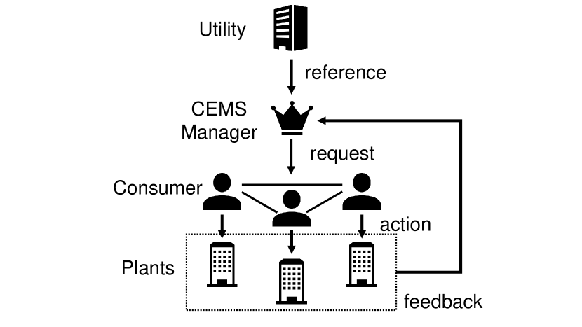
This paper addresses the feedback structure in a community-level energy management system (CEMS), which is illustrated in Fig. 1. In the figure, a power utility sends the reference of power-saving amount to the CEMS manager, and the manager provides some request to consumers. Then, the consumers take their power-saving actions to their plant systems individually. In the CEMS, we particularly pursue the following two aims: one is the reliable feedback control of accurately achieving any target power-saving amount. The other is the consumer-preferred structure of allowing consumers their selfish decisions of power-saving amount.

The key to realize the consumer-preferred structure is weak control, the concept of which is originally proposed by Inoue and Gupta (2019): the request sent from the manager to the consumers is given by the allowable range of power-saving amount, which is modeled by a set-valued signal. Then, the consumers decide the power-saving amount based on their own private preference. The decision can be made without taking care of the stability or control performance of the overall CEMS. In this paper, we address the design problem of the controllers that generate the set-valued signals. The controller structure is based on internal model control (IMC, see e.g., the book by Morari and Zafiriou (1989)). The consumer-independent stability and the worst-case control performance of the overall CEMS are studied. Finally, a numerical experiment of the consumer-preferred CEMS is performed to demonstrate the design procedure of the controller and to show its effectiveness.

Figure 1: Consumer-preferred CEMS

The remainder of this paper is organized as follows. Section 2 presents the problem setting of the CEMS design. Section 3 is devoted to the controller design and the analysis of the overall CEMS. In Section 4, a demonstration of the CEMS is given. Section 5 gives the conclusion of this paper.

Notation: The symbol ${\bf 1}_{n}$ represents the all-one vector defined in $\mathbb{R}^{n}$. For any signal $x(t)$, the symbol $x(s)$ denotes the Laplace transformation. For any $L_{2}$-signal $x(t)$, which is denoted by $x(t)\in L_{2}$, the symbol $\|x\|_{L_{2}}$ represents the $L_{2}$ norm. For any $L_{2}$-stable system $G$, the symbol $\|G\|_{L_{2}}$ represents the $L_{2}$ gain. For any rational, proper, and stable transfer matrix $G(s)$, which is denoted by $G(s)\in RH_{\infty}$, the symbol $\|G(s)\|_{H_{\infty}}$ represents the $H_{\infty}$ norm. It holds that $\|G(s)\|_{H_{\infty}}=\|G\|_{L_{2}}$.

2 Problem Setting

In this section, we consider the CEMS that includes the decision making and actions by consumers. Fig. 2 shows the block diagram of the overall structure of the CEMS. In the figure, $G$, $H$, and $K$ represent the plant set, consumer set, and controller, respectively. Note that $G$ and $H$ contain various plant systems $G_{i},i\in\{1,2,\ldots,n\}$ and various consumers $H_{i},i\in\{1,2,\ldots,n\}$, respectively. Each consumer $H_{i}$ is responsible for controlling his/her own plant $G_{i}$. In this paper, we address the design problem of $K$ for given $G$ and $H$. The model of $G$, $H$, and $K$ are given as follows.

Figure 2: Overall structure of CEMS

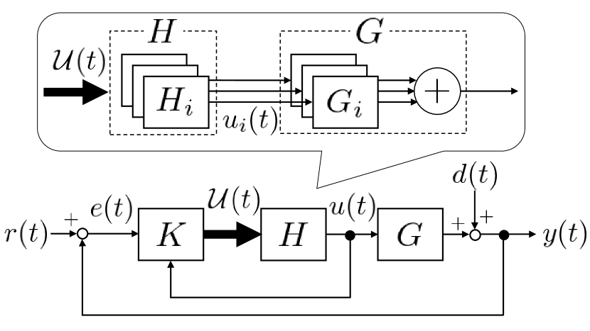
The plant set $G$ is a dynamical system, and it determines the actual power-saving amount, denoted by $y(t)\in\mathbb{R}$, based on the control action for power-saving, denoted by $u(t)\in\mathbb{R}^{n}$. In addition, let $d(t)\in\mathbb{R}$ denote the disturbance to the power-saving amount. Then, the model of $G$ is described by the following transfer function representation:

$$G:~{}y(s)=G(s)u(s)+d(s),$$ (1)

where $G(s)$ is the transfer matrix given by

$$G(s)=[\,G_{1}(s)\ G_{2}(s)\ \cdots\ G_{n}(s)\,]$$ (2)

and each of $G_{i}(s)$, $i\in\{1,2,\ldots,n\}$ represents the transfer function of $G_{i}$. For simplicity, $y(t)$, $u(t)=[\,u_{1}(t)\cdots u_{n}(t)\,]^{\top}$, and $d(t)$ are called the output, action, and disturbance, respectively. We consider that each $G_{i}$ is composed of electrical equipments and that the action $u_{i}(t)$ is to provide the set point of power-saving amount to $G_{i}$. Furthermore, it is assumed that the output of each $G_{i}$ tracks the set point at the steady state. Then, $G(s)\in RH_{\infty}$, and the following technical assumption on the steady-state property is imposed on $G$.

Assumption 1

It holds that $G(0)={\bf 1}_{n}^{\top}$.

The consumer set $H$ decides the action $u(t)$ based on the set of allowable control actions $\mathcal{U}(t)\subset\mathbb{R}^{n}$, which is requested from the controller $K$ and is modeled by a set-valued signal. The allowable set $\mathcal{U}(t)$ is called the request in the remainder of this paper. The concept of controlling decision makers by providing the set-valued control signal is called weak control (see the original work by Inoue and Gupta (2019)). For any time $t$, the decision made by $H$ is modeled by the following optimization:

$$H:\left\{\begin{array}[]{ll}\underset{u(t)}{\rm{min}}&f(t,u(t)),\\ {\rm subject~{}to}&u(t)\in\mathcal{U}(t),\\ {}&g_{1}(t,u(t))=0,\\ {}&g_{2}(t,u(t))\leq 0.\\ \end{array}\right.$$ (7)

Note here that the functions $f(t,u(t))$, $g_{1}(t,u(t))$, and $g_{2}(t,u(t))$ can be time-varying and private, i.e., they are not open to controller designers or system managers. The key of the optimization problem is the constraint

$$u(t)\in\mathcal{U}(t),$$ (8)

which is the rule imposed on the consumers. As long as the consumers follow the request such that (8) holds, they can pursue their own benefits by minimizing the cost $f(t,u(t))$. The minimization implies reducing their physical/mental burden caused by power-saving. It is assumed that for any $\mathcal{U}(t)$, the optimization problem (7) is feasible for some $u(t)$.

Let $r(t)\in\mathbb{R}$ and $e(t)\in\mathbb{R}$ denote the reference of the power-saving amount and the tracking error defined by $e(t):=r(t)-y(t)$, respectively. Then, the model of $K$ is described by

$$K:~{}\mathcal{U}(t)=K(e(t),u(t)),$$ (9)

where $K(e(t),u(t))$ represents a dynamical system and its details are given in Section 3. It is implicitly assumed that the action $u(t)$ made by $H$ is available in the operation of the controller $K$. This assumption plays a key role in the stability assurance of the overall CEMS, which is stated in Subsection 3.1.

This paper addresses the design problem of the controller $K$ pursuing the following two aims; 1) the accurate reference tracking for the power-saving amount under the presence of disturbance, 2) with (partially) allowing consumers their selfish actions. Let $G_{yr}$ and $G_{yd}$ denote the input-output dynamical systems from $r(t)$ to $y(t)$ and from $d(t)$ to $y(t)$, respectively. Then, Aim 1 is reduced ultimately to $G_{yr}=1$ and $G_{yd}=0$. Aim 2 is modeled in (7), where the consumers aim at minimizing the cost function without taking care of the stability or the control performance of the overall CEMS.

Note that pursuing Aim 1 is beneficial to the CEMS manager, while Aim 2 is clearly beneficial to consumers. In a point of view of the CEMS manager, the model of $H$, including $f(t,u(t))$ and $g_{j}(t,u(t))$, is unavailable for any of the design, implementation, and operation of $K$. Then, the design problem of $K$ pursuing Aims 1 and 2 is formulated in the following problem.

Problem 1

Given $G$, find $K$ such that the following two statements hold independently of $H$.

• The feedback system composed of $G$, $H$, and $K$ is stable.

• Given specific $\rho$, it holds that $\|y\|_{L_{2}}\leq\rho$ under the presence of $d(t)$.

This section states the problem of weakly controlling the consumer set $H$ by providing the request $\mathcal{U}(t)$. By the weak control, we aim at both of the stability assurance and control performance under the presence of selfish actions.

3 Controller Design

Figure 3: Block diagram of controller $K$

3.1 Controller Structure for Stability Assurance

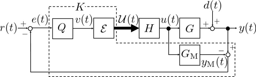
We propose the IMC-based structure in the controller $K$, which is illustrated in Fig. 3, to solve Problem 1. In the figure, the controller $K$ is composed of the plant model $G_{\rm M}$, filter $Q$, and expander $\mathcal{E}$, which are described as follows.

The plant model $G_{\rm M}$ is described by

$$G_{\rm M}:\ {y_{\rm M}(s)}=G_{\rm M}(s)u(s),$$ (10)

where $y_{\rm M}(t)\in\mathbb{R}$ is the model output, $G_{\rm M}(s)$ is the transfer matrix given by

$$G_{\rm M}(s)=[\,G_{{\rm M}1}(s)\ G_{{\rm M}2}(s)\ \cdots\ G_{{\rm M}n}(s)\,],$$ (11)

and each $G_{{\rm M}i}(s)$ represents the model of $G_{i}$.

The filter $Q$ is called the Youla parameter after the pioneering work by Youla et al. (1976). The input-output dynamics of $Q$ is described by

$$Q:\ v(s)=Q(s)e(s),$$ (12)

where $v(t)\in\mathbb{R}$ is called the filtered reference and $Q(s)$ is the transfer function satisfying $Q(s)\in RH_{\infty}$.

The expander $\mathcal{E}$ plays a central role of allowing $H$ selfish actions by generating the set-valued signal $\mathcal{U}(t)$ based on $v(t)$. The input-output behavior of $\mathcal{E}$ is described in the time-domain as

$$\mathcal{E}:\ \mathcal{U}(t)=\mathcal{E}(v(t)),$$ (13)

where $\mathcal{E}(v)$ is the set-valued function given by

$$\mathcal{E}(v)=\left\{\left.\left[\begin{array}[]{c}u_{1}\\ \vdots\\ u_{n}\end{array}\right]\right|\sum_{i=1}^{n}{{u}_{i}}=v,~{}{{u}_{i}}-\frac{1}{n}v\in[-\frac{\gamma_{{\rm l},i}}{n}v,\frac{\gamma_{{\rm u},i}}{n}v]\right\}$$ (17)

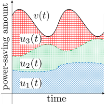
and $\gamma_{{\rm l},i}$ and $\gamma_{{\rm u},i}$ are positive constants. The center of the set-valued signal $\mathcal{U}(t)=\mathcal{E}(v(t))$ is given by $\frac{1}{n}v(t){\bf 1}_{n}$, and its volume, i.e., the degree of freedom, is characterized by the values of $\gamma_{{\rm l},i}$ and $\gamma_{{\rm u},i}$. Note that the constraint $\sum u_{i}=v$ means the resource allocation: the resource $v(t)$ is allocated to the consumers for their $u_{i}(t)$. The allocation for the case $n=3$ is illustrated in Fig. 4. The total power-saving amount of the consumers is equal to the filtered reference $v(t)$ generated by the filter $Q$.

Figure 4: Resource allocation in power-saving

The design problem of the controller $K$, which is formulated in Section 2, is reduced to the design of $Q$ and $\mathcal{E}$. The most fundamental theorem on the stability of the overall system is given.

Theorem 1

(Stability): Suppose that $Q(s)\in RH_{\infty}$ and $G_{\rm M}(s)=G(s)$. Then, the feedback system composed of $G$, $H$, and $K$ is $L_{2}$-stable independently of the model (7).

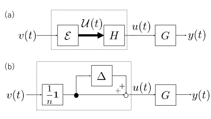
Outline of Proof of Theorem 1.  First, recall that $\frac{1}{n}v(t){\bf 1}_{n}$ is the center of $\mathcal{U}(t)$. Let $\Delta_{i}$ be the operator that outputs the error between $u_{i}(t)$ and $\frac{1}{n}v(t)$ based on the input $\frac{1}{n}v(t)$. Furthermore, we assume that $\Delta_{i}$ is in the class of the linear time-invariant (LTI) systems for simplicity of notation. Then, we have the expression

$$u_{i}(s)-\frac{1}{n}v(s)=\Delta_{i}(s)\left(\frac{1}{n}v(s)\right),$$ (18)

where $\Delta_{i}(s)$ is the transfer function of $\Delta_{i}$. Further letting

$$\Delta(s)=\rm{diag}\{\Delta_{i}(s)\},$$ (19)

it follows that the input-output system from $v(t)$ to $u(t)$ is written by

$$u(s) =({I}+\Delta(s))\left(\frac{1}{n}{\bf 1}_{n}v(s)\right).$$ (20)

The derivation of the expression (20) is illustrated in Fig. 5 (a) and (b).

Next, suppose $G_{\rm M}(s)=G(s)$. Then, the overall feedback system is described by

$$y(s)= \frac{1}{n}G(s)(I+\Delta(s)){\bf 1}_{n}Q(s)r(s)$$ (21)

$$+\left(1-\frac{1}{n}G(s)(I+\Delta(s)){\bf 1}_{n}Q(s)\right)d(s).$$ (22)

The structure of (22) is the cascaded one, i.e., $G$, $\Delta$, and $Q$ are connected in serial. Note that $\Delta$ is $L_{2}$-stable since $\|\Delta\|_{L_{2}}(=\|\Delta(s)\|_{H_{\infty}})$ is bounded by $\max\{\gamma_{{\rm l},i},\gamma_{{\rm u},i}\}$ from the definition of $\mathcal{E}(v)$ in (17). Then, noting $G(s)$, $Q(s)\in RH_{\infty}$, we show that the overall feedback system is $L_{2}$-stable. This completes the proof. ∎

Figure 5: Transformation of $\mathcal{E}$ and $H$

Remark 1

Theorem 1 claims that the stability of the overall control system is guaranteed even if any action is made by $H$. It should be emphasized that the stability is also independent of the values of $\gamma_{{\rm l},i}$ and $\gamma_{{\rm u},i}$, which determine the volume of the decision space in $H$.

3.2 Design of Youla Parameter $Q$

We propose the design strategy of $Q$ to solve Problem 1 in addition to ensuring the stability of the overall feedback system. We first briefly review the IMC-based parameter design. Then, we show that the design is also applicable to the weak control problem, stated in Problem 1.

To begin with, we suppose that $\gamma_{{\rm l},i}=\gamma_{{\rm u},i}=0$ holds for all $i\in\{1,2,\ldots,n\}$ in (17). Then, $\mathcal{U}(t)$ is described by

$$\mathcal{U}(t)=\dfrac{1}{n}{\bf 1}_{n}v(t).$$ (23)

This implies that $v(t)$ is equally distributed to $u_{i}(t)$, i.e., $u_{i}(t)=\frac{1}{n}v(t)$ holds for all $i\in\{1,2,\ldots,n\}$. Let $G_{yr}(s)$ and $G_{yd}(s)$ denote the transfer functions from $r(t)$ to $y(t)$ and from $d(t)$ to $y(t)$, respectively. Then, noting that $\Delta=0$ holds in (22), it follows that

$$G_{yr}(s) =\frac{1}{n}G(s){\bf 1}_{n}Q(s),$$ (24)

$$G_{yd}(s) =1-\frac{1}{n}G(s){\bf 1}_{n}Q(s).$$ (25)

On the basis of the classical IMC approach by Morari and Zafiriou (1989), $Q$ is designed by

$$Q(s)=\frac{nF(s)}{G_{{\rm M}}(s){\bf 1}_{n}},$$ (26)

where $F(s)$ is any filter system satisfying $F(0)=1$. It follows that $G_{yr}(s)=F(s)$ and $G_{yd}(s)=1-F(s)$ hold. This implies that the perfect tracking is achieved at the steady-state, i.e., for the step reference $r(t)\equiv r_{0}$, it holds that $y(t)\rightarrow r_{0}$, $t\rightarrow\infty$.

From now on, the weak control problem is addressed. In other words, $\gamma_{{\rm l},i}\neq\gamma_{{\rm u},i}$ holds for some $i$ in (17). Although the control performance may be deteriorated at the transient state due to the selfish actions made by $H$, the stability of the overall system is guaranteed independently of the actions as discussed in Subsection 3.1. In addition, it should be emphasized that the control performance at the steady state is NOT deteriorated compared with the case of the equal distribution (23). This fact is summarized in the following proposition.

Proposition 1

(Steady State Performance): Suppose that $Q(s)\in RH_{\infty}$ is designed by (26), $G_{\rm M}(s)=G(s)$, and $d(t)\rightarrow d_{0},t\rightarrow\infty$ for some $d_{0}$. Then, under Assumption 1, for any step reference $r(t)\equiv r_{0}$ it holds that $y(t)\rightarrow r_{0}$, $t\rightarrow\infty$ independently of the model (7).

Proof of Proposition 1. At the steady state, we see that

$$y(t) =G(0)u(t)+d_{0},$$ (27)

$$v(t) =Q(0)(r(t)-d_{0})$$ (28)

hold. From Assumption 1 and (17), it holds that

$$G(0)u(t)={\bf 1}_{n}^{\top}u(t)=v(t).$$ (29)

In addition, noting that $Q(0)=F(0)=1$ holds, we show that $y(t)\rightarrow r_{0}$, $t\rightarrow\infty$ holds. This completes the proof of the proposition. ∎

Remark 2

Proposition 1 claims that the perfect tracking to the step reference is guaranteed independently of the actions made by $H$. In other words, this steady state performance is independent of the values of $\gamma_{{\rm l},i}$ and $\gamma_{{\rm u},i}$, while the transient performance depends. In the next subsection, we address their design such that the transient error from the nominal behavior is bounded.

3.3 Design of Expander $\mathcal{E}$

In this subsection, the design problem of the expander $\mathcal{E}$ is addressed. For simplicity of discussion, consider that $r(t)\equiv 0$, i.e., only the disturbance suppression in $y(t)$ is addressed. In addition, we let

$$\gamma_{i}:=\gamma_{{\rm u},i}=\gamma_{{\rm l},i},\ i\in\{1,2\ldots,n\}$$ (30)

in (17). Then, the design problem of $\mathcal{E}$ is reduced to that of $\gamma_{i}$, $i\in\{1,2\ldots,n\}$. From the view of the CEMS manager, the aim of the design is to bound the worst case behavior in $y(t)$ caused by the actions of $H$ and the disturbance $d(t)$.

As a preliminary, we estimate the nominal behavior, where $\mathcal{U}(t)$ is given by (23) and any selfish action is not allowed for $H$. Recall the transfer function $G_{yd}(s)$ of (25). Supposing that $Q$ is designed by (26), we have $G_{yd}(s)=1-F(s)$. This results in $y(s)=d(s)-F(s)d(s)$. We let $d_{\rm f}(t)$ represent the filtered disturbance and be described in the Laplace domain by

$$d_{\rm f}(s):=F(s)d(s).$$ (31)

Then, the zero initial state response of $y(t)$ satisfies

$$\|y\|_{L_{2}}=\|d-d_{\rm f}\|_{L_{2}},$$ (32)

which is the nominal performance for the disturbance suppression.

On the basis of the estimation (32), we give the estimate of the general behavior generated in the weak control problem, where $\mathcal{U}(t)$ is given by (17) and the selfish action is partially allowed for $H$.

Proposition 2

(Disturbance Suppression): Suppose that $Q(s)\in RH_{\infty}$ is designed by (26), $G_{\rm M}(s)=G(s)$, $r(t)\equiv 0$, and $d(t)\in L_{2}$. Then, letting $\gamma_{i}$, $i\in\{1,2,\ldots,n\}$ satisfy

$$\sum_{i=1}^{n}\gamma_{i}\|G_{i}(s)\|_{H_{\infty}}\leq\frac{\varepsilon n}{\|Q(s)\|_{H_{\infty}}\|d\|_{L_{2}}}$$ (33)

for some positive constant $\varepsilon$, it holds that

$$\|y\|_{L_{2}}\leq\|d-d_{\rm f}\|_{L_{2}}+\varepsilon.$$ (34)

Proof of Proposition 2. Recall the operator $\Delta_{i}$ from the proof of Theorem 1. Here, we assume again that each $\Delta_{i}$ is LTI, which is not necessary for the proof, but avoids newly introducing redundant notation. Then, from the definition of $\mathcal{E}$ of (17), we see that

$$\|\Delta_{i}\|_{L_{2}}=\|\Delta_{i}(s)\|_{H_{\infty}}\leq\gamma_{i},\ i\in\{1,2\ldots,n\}$$ (35)

holds.

Recalling (22), which is the expression of $y(t)$ in the Laplace domain, we have

$$y(s)=d(s)-G(s)\frac{1}{n}{\bf 1}_{n}Q(s)d(s)-G(s)\Delta(s)\frac{1}{n}{\bf 1}_{n}Q(s)d(s).$$ (36)

Noting that $Q(s)$ is designed by (26), this equation is reduced to

$$y(s)=d(s)-d_{\rm f}(s)-G(s)\Delta(s)\frac{1}{n}{\bf 1}_{n}Q(s)d(s).$$ (37)

It follows that

$$\|y\|_{L_{2}} \leq\|d-d_{\rm f}\|_{L_{2}}$$ (38)

$$\quad+\frac{1}{n}\left(\sum_{i=1}^{n}\|G_{i}(s)\Delta_{i}(s)\|_{H_{\infty}}\right)\|Q(s)\|_{H_{\infty}}\|d\|_{L_{2}}.$$ (39)

We see from (33) that (34) holds. This completes the proof of the proposition. ∎

Remark 3

In Proposition 2, the performance bound of $y(t)$ is studied with respect to the designable parameters $\gamma_{i}$, $i\in\{1,2,\ldots,n\}$. The proposition states that the performance deterioration caused by any selfish actions of $H$ is bounded by $\varepsilon$. On the basis of the criterion (33), the CEMS manager can design $\mathcal{E}$, i.e., equivalently $\gamma_{i}$, $i\in\{1,2,\ldots,n\}$.

4 Numerical Demonstration

In this section, we demonstrate the design of the controller $K$ to construct the consumer-preferred CEMS. First, we give the experimental conditions including the description of the plant set $G$ and consumer set $H$. Next, for given $G$ and $H$, the controller $K$ is designed, and its effectiveness is shown.

4.1 Experimental Condition

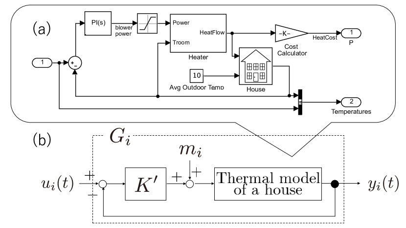
Each plant $G_{i},i\in\{1,\ldots,5\}$ represents an air conditioning system installed in a house. A part of the system is described by the thermal model in Simulink Demo (2019), MATLAB® and is illustrated in Fig. 6(a). In addition, a local controller $K^{\prime}$, which is common for all plant systems, is equipped with the thermal model. Then, a feedback system is constructed as illustrated in Fig. 6(b). The feedback system $G_{i}$ receives the signal of the power-saving action $u_{i}(t)$ and generates the power-saving amount $y_{i}(t)$. The initial state of each house is different from each other, and we let $m_{i}$ be the power consumption of each house at the initial state.

Figure 6: Structure of plant $G_{i}$

The consumer set $H$ decides the action $u(t)$ based on the request $\mathcal{U}(t)$. Let

$$c_{i}(u_{i}):=u_{i}^{2}+{6}iu_{i}$$ (40)

be the private cost function of each consumer $H_{i}$. Then, letting $m:=[\,m_{1}\cdots m_{5}\,]^{\top}$, the model of $H$ is described as follows.

$$H:\left\{\begin{array}[]{ll}\underset{u}{\rm{min}}&f(t,u(t)):=\sum_{i=1}^{5}c_{i}(u_{i}(t)),\\ {\rm subject~{}to}&u(t)\in\mathcal{U}(t),\\ {}&g_{2}(t,u(t)):=\left[\begin{array}[]{c}{u(t)-0.2m}\\ {-u(t)}\end{array}\right]\leq 0.\\ \end{array}\right.$$ (46)

The increase of the value of $c_{i}(u_{i})$ expresses the high burden imposed on each consumer. Hence, a smaller value of $f(t,u(t))$ is preferred for the consumers. The constraint $g_{2}(t,u(t))\leq 0$ means that the action of the power-saving by $H_{i}$, denoted by $u_{i}(t)$, is limited in 20 % of the initial power consumption $m_{i}$ or less.

We consider that some consumers who do not participate in CEMS affect the total power consumption. Their effects to the total power-saving amount is modeled by the disturbance $d(t)$. In this demonstration, the disturbance is given by the filtered normal random number with the average of 0 and the variance of 10. The filter $F_{d}(s)$ is given by $F_{d}(s)={1}/({10s+1})$.

In this demonstration, we consider two cases; A) the decision making and selfish actions are NOT allowed for $H$, and the power-saving request is equally distributed, i.e., $\mathcal{U}(t)$ is given by (23), and B) the decision making and selfish actions are partially allowed for $H$, and the request from the controller $K$ includes some degree of freedom, i.e., $\mathcal{U}(t)$ is given by (17).

4.2 Design of Controller $K$

The controller $K$ is designed based on the IMC structure as illustrated in Fig. 3. Then, $K$ is composed of $G_{\rm M}$, $Q$, and $\mathcal{E}$.

Initially, we obtained the plant model $G_{\rm M}$ by a system identification experiment where the step response experiment was performed for each $G_{{\rm M}i}$ independently. We found that every output followed the step input immediately. Hence, we obtained the simplistic plant model $G_{{\rm M}i}(s)=1,i\in\{1,\ldots,5\}$ in this demonstration.

In addition, we designed the low-pass filter $F(s)$ as

$$F(s) =\frac{1}{1.5s+1}.$$ (47)

By utilizing $G_{{\rm M}_{i}}(s)=1$ and this $F(s)$, the Youla parameter $Q(s)$ was designed by (26).

The expander $\mathcal{E}$ was designed as (23) in Case A), while it was designed as

$$\mathcal{E}(v)=\left\{\left.\left[\begin{array}[]{c}{u_{1}}\\ \vdots\\ {u_{n}}\end{array}\right]\right|\sum_{i=1}^{n}{u_{i}}=v\right\},$$ (51)

in Case B).

4.3 Result

Figure 7: Total power-saving amount achieved in Cases A) and B)

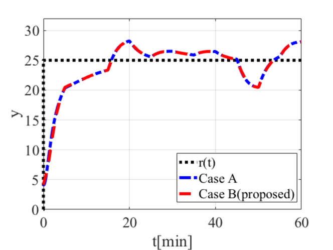
The results of the power-saving experiments by applying the two controllers A) and B) are illustrated in Fig. 7. The black dotted, red chained, and blue broken lines represent the reference and the resulting total power-saving amount in Cases A) and B), respectively. As illustrated in the figure, there is no significant difference in the performance for the reference tracking and disturbance suppression. To see this fact, the tracking error $y(t)-r(t)$ is evaluated for Cases A) and B). Letting $k$ denote the discrete time, it holds that

$$\sqrt{\sum_{k=1}^{60}(y(k)-r(k))^{2}}=36.723$$ (52)

for the both cases. This concludes that the selfish decision by the consumers does not deteriorate the overall tracking performance in the CEMS.

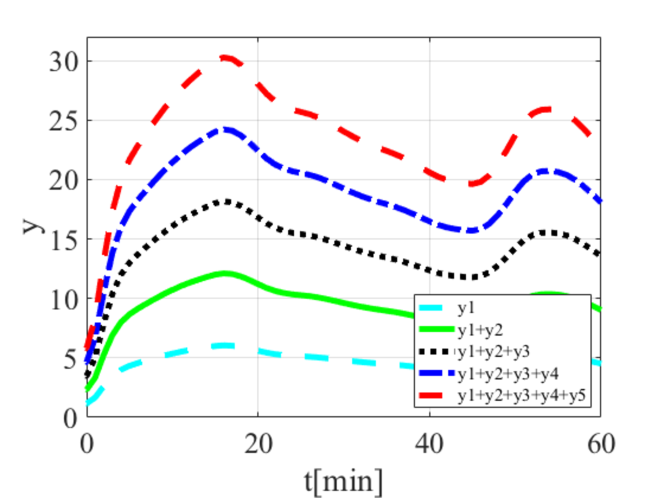
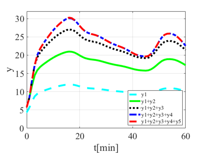
The actual power-saving amount of each plant $G_{i}$ in Cases A) and B) are illustrated in Figs. 8 and 9, respectively. Each line shows the actual power-saving amount by the consumers, denoted by $y_{1}(t)$, $y_{1}(t)+y_{2}(t)$, $\ldots$, $\sum_{i}^{5}y_{i}(t)$. In other words, the lowest, light blue chained line shows the power-saving amount $y_{1}(t)$. The second lowest, green line shows $y_{1}(t)+y_{2}(t)$. The third lowest, black dotted line shows $y_{1}(t)+y_{2}(t)+y_{3}(t)$, and so on. In Fig. 8, we see that the power-saving amount is equally distributed to the consumers. On the other hand, in Fig. 9, the amount is different from each other. The consumer $H_{1}$, who has the lowest cost for the power-saving, most contributes to the power-saving, while $H_{5}$, who has the higher cost, almost does not contribute.

Figure 8: Power-saving amount of each consumer in Case A)

Figure 9: Power-saving amount of each consumer in Case B)

Figure 10: Cost of CEMS achieved in Cases A) and B)

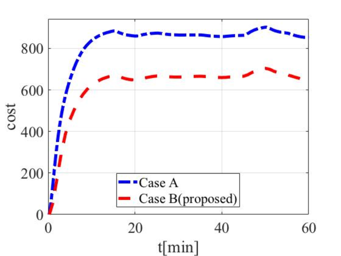
The time trajectory of the total cost $\sum_{i=1}^{5}c_{i}({y_{i}(t)})$ is illustrated in Fig. 10. The red chained and blue broken lines represent the trajectory in Cases A) and B), respectively. This figure shows the total cost is reduced in Case B) compared with Case A). We see that the the proposed weak controller, given in Section 3, is beneficial for consumers.

This experiment shows that the proposed controller contributes to reducing the private cost of consumers, while keeping the control performance within a specified allowable range.

5 Conclusion

We proposed the consumer-preferred CEMS, in which the system manager partially allowed consumers their selfish actions of power-saving while achieving desired power-saving amount. The design problem of the CEMS controller was formulated and addressed. Then, the stability, the tracking performance at the steady state, and the disturbance suppression performance at the transient state were studied and stated in Theorem 1 and Propositions 1 and 2, respectively. Finally, a numerical demonstration was performed. It was shown that the proposed controller is beneficial to consumers in addition to achieving the accurate system management.

References

- Albadi and El-Saadany (2008) Albadi, M.H. and El-Saadany, E.F. (2008). A summary of demand response in electricity markets. Electric Power Systems Research, 78(11), 1989–1996.
- Caron and Kesidis (2010) Caron, S. and Kesidis, G. (2010). Incentive-based energy consumption scheduling algorithms for the smart grid. In Proceedings of the First IEEE International Conference on Smart Grid Communications, 391–396. IEEE.
- Dobakhshari and Gupta (2018) Dobakhshari, D.G. and Gupta, V. (2018). A contract design approach for phantom demand response. IEEE Transactions on Automatic Control, 64(5), 1974–1988.
- He et al. (2018) He, J., Zhao, C., Cai, L., Cheng, P., and Shi, L. (2018). Practical closed-loop dynamic pricing in smart grid for supply and demand balancing. Automatica, 89, 92–102.
- Inoue and Gupta (2019) Inoue, M. and Gupta, V. (2019). “Weak” control for human-in-the-loop systems. IEEE Control Systems Letters, 3(2), 440–445.
- Khalid et al. (2018) Khalid, A., Javaid, N., Guizani, M., Alhussein, M., Aurangzeb, K., and Ilahi, M. (2018). Towards dynamic coordination among home appliances using multi-objective energy optimization for demand side management in smart buildings. IEEE Access, 6, 19509–19529.
- Logenthiran et al. (2012) Logenthiran, T., Srinivasan, D., and Shun, T.Z. (2012). Demand side management in smart grid using heuristic optimization. IEEE Transactions on Smart Grid, 3(3), 1244–1252.
- Miyazaki et al. (2019) Miyazaki, K., Kobayashi, K., Azuma, S.I., Yamaguchi, N., and Yamashita, Y. (2019). Design and value evaluation of demand response based on model predictive control. IEEE Transactions on Industrial Informatics.
- Mohsenian-Rad et al. (2010) Mohsenian-Rad, A.H., Wong, V.W., Jatskevich, J., and Schober, R. (2010). Optimal and autonomous incentive-based energy consumption scheduling algorithm for smart grid. In Proceedings of the 2010 Innovative Smart Grid Technologies, 1–6. IEEE.
- Morari and Zafiriou (1989) Morari, M. and Zafiriou, E. (1989). Robust Process Control. Prentice Hall.
- Palensky and Dietrich (2011) Palensky, P. and Dietrich, D. (2011). Demand side management: Demand response, intelligent energy systems, and smart loads. IEEE Transactions on Industrial Informatics, 7(3), 381–388.
- Qureshi et al. (2014) Qureshi, F.A., Gorecki, T.T., and Jones, C.N. (2014). Model predictive control for market-based demand response participation. in Preprints of the 19th IFAC World Congress, 47(3), 11153–11158.
- Rahmani-andebili (2016) Rahmani-andebili, M. (2016). Modeling nonlinear incentive-based and price-based demand response programs and implementing on real power markets. Electric Power Systems Research, 132, 115–124.
- Siano (2014) Siano, P. (2014). Demand response and smart grids survey. Renewable and Sustainable Energy Reviews, 30, 461–478.
- Simulink Demo (2019) Simulink Demo (2019). Thermal model of a house. ”https://jp.mathworks.com/help/simulink/slref/thermal-model-of-a-house.html”.
- Strbac (2008) Strbac, G. (2008). Demand side management: Benefits and challenges. Energy Policy, 36(12), 4419–4426.
- Youla et al. (1976) Youla, D., Bongiorno, J.d., and Jabr, H. (1976). Modern Wiener–Hopf design of optimal controllers Part I: The single-input-output case. IEEE Transactions on Automatic Control, 21(1), 3–13.