Discontinuous transitions can survive to quenched disorder in a two-dimensional nonequilibrium system

Abstract

We explore the effects that quenched disorder has on discontinuous nonequilibrium phase transitions into absorbing states. We focus our analysis on the Naming Game model, a nonequilibrium low-dimensional system with different absorbing states. The results obtained by means of the finite-size scaling analysis and from the study of the temporal dynamics of the density of active sites near the transition point evidence that the spatial quenched disorder does not destroy the discontinuous transition.

I Introduction

The study of nonequilibrium models is currently an important topic of statistical physics odor0 ; odor . The theory of phase transitions in equilibrium systems is well established and rests upon solid foundations, with numerous results rigorously proved. Moreover, it has been thoroughly tested and validated through a large number of empirical and numerical evidence. In contrast, work on the development of a similar theory for nonequilibrium systems is rather recent, and results are often limited in scope and lack adequate validation odor0 ; odor . For this reason, one is sometimes led to apply most of the fundamental equilibrium results to nonequilibrium systems following simple analogies or heuristic generalizations. The question of whether some specific result of equilibrium statistical mechanics can be effectively extended to nonequilibrium systems is open for a number of different issues. In this paper we will focus on an important result of equilibrium statistical physics, which states that the introduction of quenched random fields or interactions in low-dimensional ($d\leq 2$) systems causes the disappearance of discontinuous phase transitions equilibrium . Quenched randomness precludes the presence of such types of transitions.

In a recent work Villa Martín et al. villa addressed the question whether such result can be translated to the nonequilibrium realm. They studied a two-dimensional reaction-diffusion contact-process-like model odor0 ; odor , a very simple nonequilibrium model with one absorbing state which exhibits a discontinuous transition. They showed that the introduction of disorder annihilated the discontinuous phase transition and induced a continuous one, just as what should be expected in the equilibrium case. This result led to the conjecture that the arguments used in equilibrium systems could be extended to nonequilibrium ones, leading to the disappearance of the discontinuous phase transitions, due to quenched disorder, in general low-dimensional nonequilibrium systems with absorbing states villa .

Intrigued by this fascinating idea, we test here this hypothesis by means of a recently introduced nonequilibrium model with absorbing states: the Naming Game model baronchelli06 . This model is related to the large family of models which implement an ordering dynamics that may generate global consensus as an emergent phenomenon among interacting agents. Despite its simplicity, its collective dynamics present new features not commonly found in other more traditional models. In fact, these dynamics rests on a memory-based negotiation, where trials shape and reshape the memories, allowing for intermediate individual states, feedback phenomena, and dynamic inventories. This model generated a vivid interest because some of its variants were able to describe different aspects of linguistic dynamics, like, for example, the birth of neologisms baronchelli06 , the effects of reputation on fixing vocabulary edo1 , the self-organization of a hierarchical category structure apply1 , the emergence of universality in color naming patterns apply2 , the duality of patterning in human communication apply3 , and the rise of protosyntactic structures apply4 .

Some versions of the model display a discontinuous phase transition baronchelli07 ; eddy . This behavior can be obtained by the introduction of a specific control parameter which represents the efficiency of the communication process, accounting for external or internal influences or agents’ irresolute attitude baronchelli07 . This ingredient generates a transition between an absorbing state of global consensus and a stationary state with several coexisting conventions. The richness of the Naming Game model, which moves a step further from the simplicity of the contact process, does not preclude the possibility of describing it with methods borrowed from classical equilibrium statistical mechanics. This fact could be appreciated in previous studies which clearly characterized its phase transition baronchelli07 ; nos .

II The model

We simulate the game on a regular two-dimensional (2D) square lattice with periodic boundary conditions, where only nearest-neighbor pairs of sites are considered in the rules of the game. At each of the $L\times L$ sites an agent, or player, is placed. It is characterized by an inventory which can store an infinite number of conventions. This inventory is structured as an array of potentially infinite cells, where each cell is set on one of a countable infinite number of possible states. Every player starts with an empty inventory. At each time step, a pair of agents is randomly selected. The first agent selects one of its conventions or creates a new one, if its inventory is empty. After that, the convention selected is transmitted to the second agent. If this last agent already possesses in its own inventory the convention transmitted, the two agents involved in the interaction update their inventories so as to keep only the considered convention, with a probability $\beta$. Conversely, no action is performed by the couple of agents, with probability $1-\beta$. Otherwise, if the second agent does not already possess the transmitted convention, the interaction is a failure, and it adds the new convention to its own inventory. If $\beta=1$, the model coincides with the original Naming Game baronchelli06 implemented on a low-dimensional lattice. This model always converges to an absorbent ordered state characterized by one single convention adopted by every agent baronchelli06b . When the behavior of the model is studied as a function of the parameter $\beta$, a transition between overall consensus and several coexisting conventions appears, driven by the value of the parameter. The critical value $\beta_{c}$ is close to 1/3 for the mean-field model baronchelli07 and $\beta_{c}=0.329\pm 0.001$ on a regular 2D lattice nos . Moreover, this last study shows, by means of a rigorous finite-size scaling analysis, that the model effectively displays a discontinuous nonequilibrium phase transition with absorbing states nos .

This pure model can be modified to obtain a disordered version. In this version, the parameter that controls the outcome of each interaction is no longer the same for all agents. Each agent $i$ is now characterized by a random uncorrelated probability $\beta_{i}$, where we take $\beta_{i}=\beta+r$ where $\beta$ is constant and $r$ is a random number on the interval $[-\eta,+\eta]$ chosen with a uniform probability. The values of $\beta_{i}$ are thus randomly defined and fixed at the beginning of each simulation.

III Results and discussion

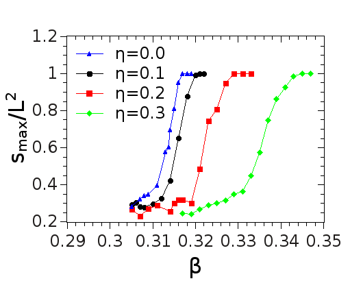
Figure 1: Characterization of the phase transition using the mean of the normalized largest cluster size as a function of $\beta$. Results are displayed for different levels of noise ($\eta$). Each point is averaged over $100$ simulations, $L=40$.

As a first step, we analyze the differences generated in the general form of the phase transition by the introduction of the quenched noise. The phase transition corresponds to the shift from an active stationary state, characterized by disordered and fragmented clusters, to an absorbing state made of a single cluster represented by the same convention. Because of this phenomenology, the relative size of the largest cluster present in the system is an excellent parameter that characterizes the transition castellano00 ; brigatti15 . This parameter is defined as the size of the largest cluster, made up by the agents sharing the same unique convention, normalized by the system size: $s_{max}/L^{2}$. This parameter is estimated once the steady state is reached and it is averaged over different simulations: $\langle s_{max}/L^{2}\rangle$. As the system presents very slow relaxation time close to the transition, we have to run very long simulations ($4\times 10^{10}$ Monte Carlo steps) which forced us to adopt $L$ values only up to 100. In Figure 1 we can observe how the introduction of noise, controlled by the parameter $\eta$, impacts the transition behavior. The critical value of $\beta_{c}(L)$ is shifted towards higher $\beta$ values but, surprisingly, the discontinuous phase transitions are not clearly rounded by disorder, a fact that generates some doubts about the potentiality of noise in generating a continuous transition.

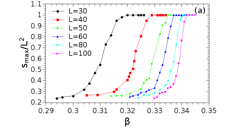
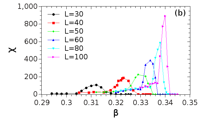
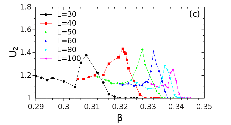
Figure 2: From top to bottom: (a) Mean of the normalized largest cluster size, (b) its variance $\chi$ and (c) the moment ratio $U_{2}$ as a function of $\beta$ for different system sizes and $\eta=0.2$. Each point is averaged over up to $200$ simulations.

For this reason we turn our attention to a rigorous characterization of the phase transition, based on a finite-size scaling analysis. In fact, the scaling behavior of the system near the transition can clearly discriminate between a continuous or discontinuous transition.

We performed the analysis evaluating the fluctuations of the size of the largest cluster:

$$\chi=L^{2}(\langle s_{max}^{2}\rangle-\langle s_{max}\rangle^{2})$$

and its moment ratio (reduced cumulant) dickman98 :

$$U_{2}=\frac{\langle s_{max}^{2}\rangle}{\langle s_{max}\rangle^{2}};$$

for different $L$ values.

As can be appreciated in Figure 2, these quantities peak at around $\beta_{c}(L)$. Actually, the use of the maxima of these quantities has proven to be a very efficient method for performing finite size scaling analysis of discontinuous phase transition into absorbing states oliveira2015 . In this case, the asymptotic transition point can be obtained by looking at the convergence of the finite size transition points $\beta_{c}(L)$, as estimated by the localization of the maxima of the fluctuations or the maxima of the moment ratio. In both cases, the convergence is expected to follow an algebraic behavior: $\beta_{c}(L)=\beta_{c}+aL^{-2}$, which is the usual equilibrium scaling for discontinuous transitions oliveira2015 ; mio19 ; privman . Our data follow these scaling laws very well: Figure 3 shows how the maxima positions for $\chi$ and $U_{2}$ effectively decrease as $1/L^{2}$. An extrapolation for $L\to\infty$ yields $\beta_{c}=0.342\pm 0.001$ for $\chi$ and $\beta_{c}=0.341\pm 0.001$ for $U_{2}$, two very close values.

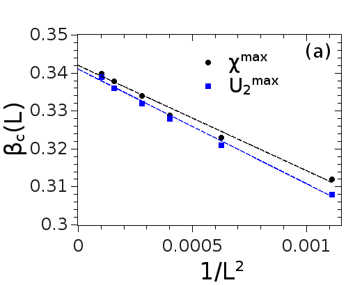
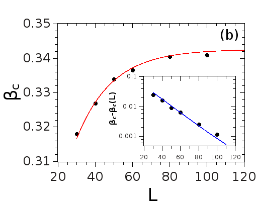
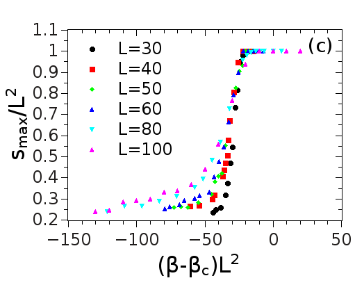
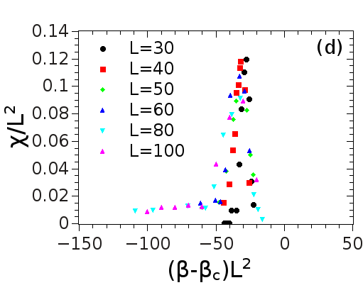
Figure 3: Top: (a) Convergence to the asymptotic transition point $\beta_{c}$ of the finite-size transition points $\beta_{c}(L)$ measured from the variance and the $U_{2}$ maxima. (b) Convergence to the asymptotic transition point $\beta_{c}$ of the finite-size transition points $\beta_{c}(L)$ measured from the jump location in the normalized size of the largest cluster. The continuous line represents the best fitting function: $\beta_{c}(L)=0.343-0.125\exp(-0.052L)$. In the inset, the semilogarithmic plot shows in detail the expected exponential behavior of the difference $\beta_{c}-\beta_{c}(L)$. Bottom: (c) Rescaled plot for $\langle s_{max}\rangle/L^{2}$ and (d) its fluctuations.

An alternative approach borgs for the estimation of the asymptotic transition point uses the location of the observed discontinuity in the normalized size of the largest cluster (the first value of $\beta$ for which $\langle s_{max}\rangle/L^{2}$ is smaller than $1$). Using this method the convergence is supposed to be exponential and the extrapolation for $L\to\infty$ gives $\beta_{c}=0.343\pm 0.002$ (see Figure 3). In the same figure we can observe how the difference $\beta_{c}-\beta_{c}(L)$ clearly presents the expected exponential behavior.

Additional consistency checks of the above results can be performed verifying whether the measured quantities present the typical scaling of a discontinuous transition near the transition point, a standard procedure for equilibrium finite-size scaling analysis binder ; oliveira2015 . The scaling plot of $\langle s_{max}\rangle/L^{2}$ should be obtained introducing the rescaled control parameter $\beta^{*}=(\beta-\beta_{c})L^{d}$, where $d$ is the system dimension. Similarly, the scaling plot of the fluctuations should be drawn using the rescaled fluctuations $\chi\cdot L^{-d}$ and the rescaled parameter $\beta^{*}$. Figure 3 shows a reasonable collapse which satisfies these relations, strongly suggesting the validity of the finite-size scaling ansatz expected for a discontinuous transition.

An alternative way for differentiating between continuous and discontinuous transition is based on the distinct behavior of the temporal dynamics of the density of active sites. In our model such density corresponds to the fraction $\rho$ of agents presenting more than one convention in their inventories lipowska . Near the transition point the density is expected to decay smoothly to zero in the case of continuous phase transitions and to develop an abrupt discontinuous jump in the case of discontinuous transitions. In particular, in continuous phase transitions the density of active sites typically presents a power-law decay odor . Even so, some models which present continuous transitions between active and absorbing states are characterized by slower decays (logarithmic) of active sites (for example, in voter-like models 22 and in Potts model with absorbing states 23 ).

We collected some numerical data depicting the dynamics of the density of active sites for our model with quenched disorder. A clear representation of the density evolution can be obtained averaging over many independent runs. Before calculating these averages, since the convergence time in this model is characterized by a very wide distribution, it is useful to shift each time series $i$ by the time $t^{0}_{i}$, which corresponds to the time when the density $\rho_{i}$ goes to zero. As can be seen in Figure 4, the time evolution of the density of active sites clearly develops an abrupt discontinuous jump, corroborating the view that the transition is discontinuous.

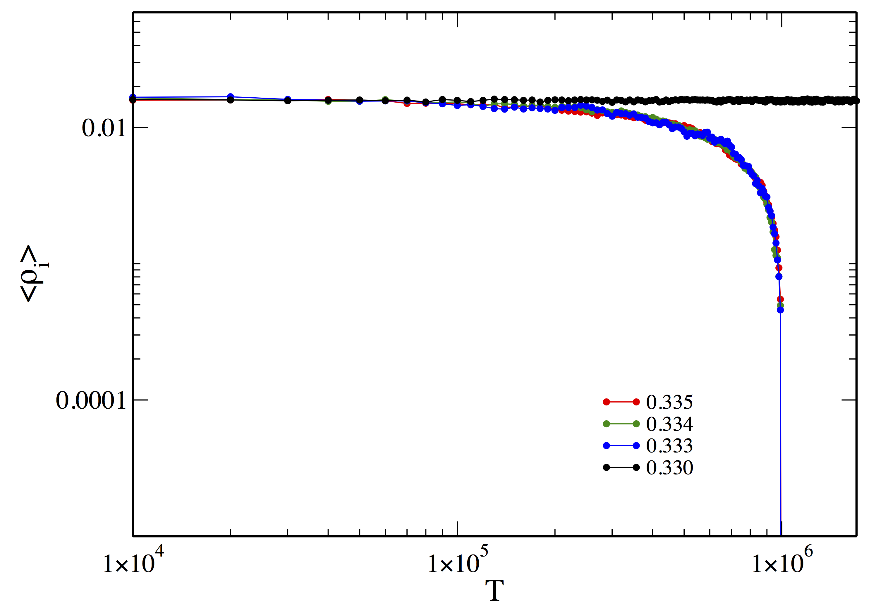
Figure 4: Time evolution of the density of multi-convention agents for different values of $\beta$, $\eta=0.2$, and $L=60$. The rescaled time $T=(t-t^{0}_{i})+10^{6}$, where $t$ is the Monte Carlo step and $t^{0}_{i}$ corresponds to the step when the density $\rho_{i}$ goes to zero. Points represent the ensemble average of $\rho_{i}$, obtained considering only the simulations which converged to the consensus state. For $\beta=0.330$, the time is not rescaled and the average is over all the simulations.

In summary, we have numerically studied the effects of introducing a spatial quenched disorder in a Naming Game model which, in its pure version, presents a well known discontinuous phase transition.The aim of the analysis is to state whether the presence of the quenched randomness results in the disappearance of the discontinuous phase transition, as is known to happen in equilibrium systems. In contrast to this conjecture, our analysis suggests that the model maintains the discontinuous phase transition. This conclusion is supported by the evidence provided by the results of a finite-size scaling analysis. We found that, as for the pure (without disorder) model, the behavior of the finite-size transition points measured from the variance, the moment ratio or, the jump locations show a scaling behavior which can be associated with a discontinuous transition. Additional confirmations of these results come from the collapse of the scaling plot of the order parameter and its fluctuations which have been obtained using the scaling law expected for a discontinuous transition oliveira2015 . Moreover, the temporal dynamics of the density of the active sites near the transition point develops an abrupt discontinuous jump, as expected in the case of discontinuous transitions. These numerical results constitute evidence for the survival of the discontinuous phase transition after the introduction of quenched disorder.

Previous works have already shown that temporal disorder does not destroy discontinuous transitions in a variety of two-dimensional models fiore . In our study, the transition surprisingly survives also in the case of a simple quenched spatial disorder. It is interesting to note that the model considered in villa , for which the discontinuous transition disappeared, is characterized by only one absorbing state. In contrast, our model presents a large number of possible different absorbing states.

We conclude our work by proposing a heuristic argument for explaining the phenomenology behind this single-multiple absorbing states dichotomy in rounding (or not) the discontinuous transition. An interesting inspiration comes from the case of continuous phase transitions. In that scenario the result that random fields destroy an equilibrium phase transition in low dimensions ma cannot be transposed to nonequilibrium systems. This fact was shown by the analysis of Barghathi et al., where the phase transition of a generalized contact process presenting two absorbing states persists in the presence of disorder barga . In such an example the existence of two absorbing states is essential. In fact, along its dynamics the system organizes in distinct uniform domains corresponding to the two absorbing states and neither active sites nor new domains can arise in the interior of a given domain, as its states are inactive. After a process of coalescence of these domains, in the long-time limit, the system reaches a single-domain state. In contrast, in the equilibrium case of a random-field Ising model, the growth of a uniform domain is limited by spin flips which can occur anywhere due to fluctuations. The domains size reaches a typical value controlled by the Imry-Ma argument ma , suppressing the continuous transition. The case of the discontinuous transition can be explained following the work of Kardar et al. kardar which suggests that disorder precludes discontinuous transitions by generating islands of arbitrary size of one of the phases within the other. This nested structure of islands within islands leads to the formation of hybrid states and two distinct phases cannot coexist. This phenomenon can happen in the contact-process-like model considered in villa , where the unique absorbing state corresponding to no-particle occupation can pop-up everywhere in the system, as particles disappear at random locations. In contrast, in our model, once a domain with a specific inactive state is defined, it is not possible to create smaller regions in the opposite phase inside it, paralyzing this mechanism and allowing the discontinuous transition to take place.

References

- (1) J. Marro and R. Dickman, Nonequilibrium Phase Tran- sitions in Lattice Models, (Cambridge University Press, Cambridge, 1999); M. Henkel, H. Hinrichsen, and S. Lübeck, Non-Equilibrium Phase Transitions, Volume I: Absorbing Phase Transitions, (Springer, New York, 2008).
- (2) G. Ódor, Rev. Mod. Phys. 76, 663 (2004).
- (3) M. Aizenman and J. Wehr, Phys. Rev. Lett. 62, 2503 (1989); A. N. Berker, Phys. A 194, 72 (1993); K. Hui and A. N. Berker, Phys. Rev. Lett. 62, 2507 (1989).
- (4) P. Villa Martín, J. A. Bonachela and M. A. Muñoz, Phys. Rev. E 89, 012145 (2014).
- (5) A. Baronchelli, M. Felici, E. Caglioti, V. Loreto and L. Steels, J. Stat. Mech. P06014 (2006).
- (6) E. Brigatti, Phys. Rev. E 78, 046108 (2008).
- (7) A. Puglisi, A. Baronchelli and V. Loreto, Proc. Natl. Acad. Sci. 105, 7936 (2008).
- (8) A. Baronchelli, T. Gong, A. Puglisi and V. Loreto, Proc. Natl. Acad. Sci. 107, 2403 (2010).
- (9) F. Tria, B. Galantucci, and V. Loreto, Plos One 7, 0037744 (2012).
- (10) E. Brigatti, Phys. Rev. E 86, 026107 (2012).
- (11) A. Baronchelli, L. Dall’Asta, A. Barrat and V. Loreto, Phys. Rev. E 76, 051102 (2007).
- (12) E. Brigatti and I. Roditi, New J. Phys. 11, 023018 (2009).
- (13) E. Brigatti and A. Hernández, Phys. Rev. E 94, 052308 (2016).
- (14) A. Baronchelli, L. Dall’Asta, A. Barrat and V. Loreto, Phys. Rev. E 73, 015102(R) (2006).
- (15) C. Castellano, M. Marsili and A. Vespignani, Phys. Rev. Lett. 85, 3536 (2000).
- (16) N. Crokidakis and E. Brigatti, J. Stat. Mech., P01019 (2015).
- (17) R. Dickman and J. Kamphorst Leal da Silva, Phys. Rev. E 58, 4266 (1998).
- (18) M. M. de Oliveira, M. G. E. da Luz and C. E. Fiore, Phys. Rev. E 92, 062126 (2015).
- (19) A.M. Calvão, E. Brigatti , Physica A 520, 450 (2019).
- (20) V. Privman, Finite Size Scaling and Numerical Simulations of Statistical Systems, (World Scientific, Singapore, 1990); S. W. Sides, P. A. Rikvold and M. A. Novotny, Phys. Rev. Lett. 81, 834 (1998).
- (21) C. Borgs and R. Kotecky, J. Stat. Phys. 61, 79 (1990); Phys. Rev. Lett. 68, 1734 (1992); H. Chaté, F. Ginelli, G. Grégoire, F. Raynaud, Phys. Rev. E 77, 046113 (2008).
- (22) K. Binder and D. P. Landau, Phys. Rev. B 30, 1477 (1984); K. Binder, Z. Phys. B 43, 119 (1981).
- (23) D. Lipowska and A. Lipowski, J. Stat. Mech., P08001 (2014).
- (24) L. Frachebourg and P. L. Krapivsky, Phys. Rev. E 53 R3009(R) (1996).
- (25) A. Lipowski and M. Droz, Phys. Rev. E 65 056114 (2002).
- (26) Y.Imry and S. K. Ma, Phys. Rev. Lett. 35, 1399 (1975).
- (27) H. Barghathi and T. Vojta, Phys. Rev. Lett. 109, 170603 (2012).
- (28) M. Kardar, A.L. Stella, G. Sartoni, and B. Derrida, Phys. Rev. E 52, R1269 (1995).
- (29) M. M. de Oliveira and C. E. Fiore, Phys. Rev. E 94, 052138 (2016); C. E. Fiore, M. M. de Oliveira and J. A. Hoyos Phys. Rev. E 98, 032129 (2018).