Hebbian Synaptic Modifications in Spiking Neurons that Learn

Abstract

In this paper, we derive a new model of synaptic plasticity, based on recent algorithms for reinforcement learning (in which an agent attempts to learn appropriate actions to maximize its long-term average reward). We show that these direct reinforcement learning algorithms also give locally optimal performance for the problem of reinforcement learning with multiple agents, without any explicit communication between agents. By considering a network of spiking neurons as a collection of agents attempting to maximize the long-term average of a reward signal, we derive a synaptic update rule that is qualitatively similar to Hebb’s postulate. This rule requires only simple computations, such as addition and leaky integration, and involves only quantities that are available in the vicinity of the synapse. Furthermore, it leads to synaptic connection strengths that give locally optimal values of the long term average reward. The reinforcement learning paradigm is sufficiently broad to encompass many learning problems that are solved by the brain. We illustrate, with simulations, that the approach is effective for simple pattern classification and motor learning tasks.

1 What is a good synaptic update rule?

It is widely accepted that the functions performed by neural circuits are modified by adjustments to the strength of the synaptic connections between neurons. In the 1940s, Donald Hebb speculated that such adjustments are associated with simultaneous (or nearly simultaneous) firing of the presynaptic and postsynaptic neurons [14]:

When an axon of cell $A$ … persistently takes part in firing [cell $B$], some growth process or metabolic change takes place [to increase] $A$’s efficacy as one of the cells firing $B$.

Although this postulate is rather vague, it provides the important suggestion that the computations performed by neural circuits could be modified by a simple cellular mechanism. Many candidates for Hebbian synaptic update rules have been suggested, and there is considerable experimental evidence of such mechanisms (see, for instance, [7, 23, 16, 17, 19, 21]).

Hebbian modifications to synaptic strengths seem intuitively reasonable as a mechanism for modifying the function of a neural circuit. However, it is not clear that these synaptic updates actually improve the performance of a neural circuit in any useful sense. Indeed, simulation studies of specific Hebbian update rules have illustrated some serious shortcomings (see, for example, [20]).

In contrast with the “plausibility of cellular mechanisms” approach, most artificial neural network research has emphasized performance in practical applications. Synaptic update rules for artificial neural networks have been devised that minimize a suitable cost function. Update rules such as the backpropagation algorithm [22] (see [12] for a more detailed treatment) perform gradient descent in parameter space: they modify the connection strengths in a direction that maximally decreases the cost function, and hence leads to a local minimum of that function. Through appropriate choice of the cost function, these parameter optimization algorithms have allowed artificial neural networks to be applied (with considerable success) to a variety of pattern recognition and predictive modelling problems.

Unfortunately, there is little evidence that the (rather complicated) computations required for the synaptic update rule in parameter optimization procedures like the backpropagation algorithm can be performed in biological neural circuits. In particular, these algorithms require gradient signals to be propagated backwards through the network.

This paper presents a synaptic update rule that provably optimizes the performance of a neural network, but requires only simple computations involving signals that are readily available in biological neurons. This synaptic update rule is consistent with Hebb’s postulate.

Related update rules have been proposed in the past. For instance, the updates used in the adaptive search elements (ASEs) described in [4, 2, 1, 3] are of a similar form (see also [25]). However, it is not known in what sense these update rules optimize performance. The update rule we present here is based on similar foundations to the REINFORCE class of algorithms introduced by Williams [27]. However, when applied to spiking neurons such as those described here, REINFORCE leads to parameter updates in the steepest ascent direction in two limited situations: when the reward depends only on the current input to the neuron and the neuron outputs do not affect the statistical properties of the inputs, and when the reward depends only on the sequence of inputs since the arrival of the last reward value. Furthermore, in both cases the parameter updates must be carefully synchronized with the timing of the reward values, which is especially problematic for networks with more than one layer of neurons.

In Section 2, we describe reinforcement learning problems, in which an agent aims to maximize the long-term average of a reward signal. Reinforcement learning is a useful abstraction that encompasses many diverse learning problems, such as supervised learning for pattern classification or predictive modelling, time series prediction, adaptive control, and game playing. We review the direct reinforcement learning algorithm we proposed in [5] and show in Section 3 that, in the case of multiple independent agents cooperating to optimize performance, the algorithm conveniently decomposes in such a way that the agents are able to learn independently with no need for explicit communication.

In Section 4, we consider a network of model neurons as a collection of agents cooperating to solve a reinforcement learning problem, and show that the direct reinforcement learning algorithm leads to a simple synaptic update rule, and that the decomposition property implies that only local information is needed for the updates. Section 5 discusses possible mechanisms for the synaptic update rule in biological neural networks.

The parsimony of requiring only one simple mechanism to optimize parameters for many diverse learning problems is appealing (cf [26]). In Section 6, we present results of simulation experiments, illustrating the performance of this update rule for pattern recognition and adaptive control problems.

2 Reinforcement learning

‘Reinforcement learning’ refers to a general class of learning problems in which an agent attempts to improve its performance at some task. For instance, we might want a robot to sweep the floor of an office; to guide the robot, we provide feedback in the form of occasional rewards, perhaps depending on how much dust remains on the floor. This section explains how we can formally define this class of problems and shows that it includes as special cases many conventional learning problems. It also reviews a general-purpose learning method for reinforcement learning problems.

We can model the interactions between an agent and its environment mathematically as a partially observable Markov decision process (POMDP). Figure 1 illustrates the features of a POMDP. At each (discrete) time step $t$, the agent and the environment are in a particular state $x_{t}$ in a state space ${\cal S}$. For our cleaning robot, $x_{t}$ might include the agent’s location and orientation, together with the location of dust and obstacles in the office. The state at time $t$ determines an observation vector $y_{t}$ (from some set ${\cal Y}$) that is seen by the agent. For instance in the cleaning example, $y_{t}$ might consist of visual information available at the agent’s current location. Since observations are typically noisy, the relationship between the state and the corresponding observation is modelled as a probability distribution $\nu(x_{t})$ over observation vectors. Notice that the probability distribution depends on the state.

Figure 1: Partially observable Markov decision process (POMDP).

When the agent sees an observation vector $y_{t}$, it decides on an action $u_{t}$ from some set ${\cal U}$ of available actions. In the office cleaning example, the available actions might consist of directions in which to move or operations of the robot’s broom.

A mapping from observations to actions is referred to as a policy. We allow the agent to choose actions using a randomized policy. That is, the observation vector $y_{t}$ determines a probability distribution $\mu(y_{t})$ over actions, and the action is chosen randomly according to this distribution. We are concerned with randomized policies that depend on a vector $\theta\in{\mathbb{R}}^{k}$ of $k$ parameters (and we write the probability distribution over actions as $\mu(y_{t},\theta)$).

The agent’s actions determine the evolution of states, possibly in a probabilistic way. To model this, each action determines the probabilities of transitions from the current state to possible subsequent states. For a finite state space ${\cal S}$, we can write these probabilities as a transition probability matrix, $P(u_{t})$. Here, the $i,j$-the entry of $P(u_{t})$ ($p_{ij}(u_{t})$) is the probability of making a transition from state $i$ to state $j$ given that the agent took action $u_{t}$ in state $i$. In the office, the actions chosen by the agent determine its location and orientation and the location of dust and obstacles at the next time instant, perhaps with some random element to model the probability that the agent slips or bumps into an obstacle.

Finally, in every state, the agent receives a reward signal $r_{t}$, which is a real number. For the cleaning agent, the reward might be zero most of the time, but take a positive value when the agent removes some dust.

The aim of the agent is to choose a policy (that is, the parameters that determine the policy) so as to maximize the long-term average of the reward,

$$\eta=\lim_{T\to\infty}\mbox{\boldmath$\bf E$}\left[\frac{1}{T}\sum_{t=1}^{T}r_{t}\right].$$ (1)

(Here, $\bf E$ is the expectation operator.) This problem is made more difficult by the limited information that is available to the agent. We assume that at each time step the agent sees only the observations $y_{t}$ and the reward $r_{t}$ (and is aware of its policy and the actions $u_{t}$ that it chooses to take). It has no knowledge of the underlying state space, how the actions affect the evolution of states, how the reward signals depend on the states, or how the observations depend on the states.

2.1 Other learning tasks viewed as reinforcement learning

Clearly, the reinforcement learning problem described above provides a good model of adaptive control problems, such as the acquisition of motor skills. However, the class of reinforcement learning problems is broad, and includes a number of other learning problems that are solved by the brain. For instance, the supervised learning problems of pattern recognition and predictive modelling require labels (such as an appropriate classification) to be associated with patterns. These problems can be viewed as reinforcement learning problems with reward signals that depend on the accuracy of each predicted label. Time series prediction, the problem of predicting the next item in a sequence, can be viewed in the same way, with a reward signal that corresponds to the accuracy of the prediction. More general filtering problems can also be viewed in this way. It follows that a single mechanism for reinforcement learning would suffice for the solution of a considerable variety of learning problems.

2.2 Direct reinforcement learning

A general approach to reinforcement learning problems was presented recently in [5, 6]. Those papers considered agents that use parameterized policies, and introduced general-purpose reinforcement learning algorithms that adjust the parameters in the direction that maximally increases the average reward. Such algorithms converge to policies that are locally optimal, in the sense that any further adjustment to the parameters in any direction cannot improve the policy’s performance. This section reviews the algorithms introduced in [5, 6]. The next two sections show how these algorithms can be applied to networks of spiking neurons.

The direct reinforcement learning approach presented in [5], building on ideas due to a number of authors [27, 9, 10, 15, 18], adjusts the parameters $\theta$ of a randomized policy that, on being presented with the observation vector $y_{t}$, chooses actions according to a probability distribution $\mu(y_{t},\theta)$. The approach involves the computation of a vector $z_{t}$ of $k$ real numbers (one component for each component of the parameter vector $\theta$) that is updated according to

$$z_{t+1}=\beta z_{t}+\frac{\nabla\mu_{u_{t}}(y_{t},\theta)}{\mu_{u_{t}}(y_{t},\theta)},$$ (2)

where $\beta$ is a real number between $0$ and $1$, $\mu_{u_{t}}(y_{t},\theta)$ is the probability of the action $u_{t}$ under the current policy, and $\nabla$ denotes the gradient with respect to the parameters $\theta$ (so $\nabla\mu_{u_{t}}(y_{t},\theta)$ is a vector of $k$ partial derivatives). The vector $z_{t}$ is used to update the parameters, and can be thought of as an average of the ‘good’ directions in parameter space in which to adjust the parameters if a large value of reward occurs at time $t$. The first term in the right-hand-side of (2) ensures that $z_{t}$ remembers past values of the second term. The numerator in the second term is in the direction in parameter space which leads to the maximal increase of the probability of the action $u_{t}$ taken at time $t$. This direction is divided by the probability of $u_{t}$ to ensure more “popular” actions don’t end up dominating the overall update direction for the parameters. Updates to the parameters correspond to weighted sums of these normalized directions, where the weighting depends on future values of the reward signal.

Theorems 3 and 6 in [5] show that if $\theta$ remains constant, the long-term average of the product $r_{t}z_{t}$ is a good approximation to the gradient of the average reward with respect to the parameters, provided $\beta$ is sufficiently close to $1$. It is clear from Equation (2) that as $\beta$ gets closer to $1$, $z_{t}$ depends on measurements further back in time. Theorem 4 in [5] shows that, for a good approximation to the gradient of the average reward, it suffices if $1/(1-\beta)$, the time constant in the update of $z_{t}$, is large compared with a certain time constant—the mixing time—of the POMDP. (It is useful, although not quite correct, to think of the mixing time as the time from the occurrence of an action until the effects of that action have died away.)

This gives a simple way to compute an appropriate direction to update the parameters $\theta$. An on-line algorithm ($\operatorname{OLPOMDP}$) was presented in [6] that updates the parameters $\theta$ according to

$$\theta_{t}=\theta_{t-1}+\gamma r_{t}z_{t},$$ (3)

where the small positive real number $\gamma$ is the size of the steps taken in parameter space. If these steps are sufficiently small, so that the parameters change slowly, this update rule modifies the parameters in the direction that maximally increases the long-term average of the reward.

3 Direct reinforcement learning with independent agents

Suppose that, instead of a single agent, there are $n$ independent agents, all cooperating to maximize the average reward (see Figure 2). Suppose that each of these agents sees a distinct observation vector, and has a distinct parameterized randomized policy that depends on its own set of parameters. This multi-agent reinforcement learning problem can also be modelled as a POMDP by considering this collection of agents as a single agent, with an observation vector that consists of the $n$ observation vectors of each independent agent, and similarly for the parameter vector and action vector. For example, if the $n$ agents are cooperating to clean the floor in an office, the state vector would include the location and orientation of the $n$ agents, the observation vector for agent $i$ might consist of the visual information available at that agent’s current location, and the actions chosen by all $n$ agents determine the state vector at the next time instant. The following decomposition theorem follows from a simple calculation.

Figure 2: POMDP controlled by $n$ independent agents.

Theorem 1.

For a POMDP controlled by multiple independent agents, the direct reinforcement learning update equations (2) and (3) for the combined agent are equivalent to those that would be used by each agent if it ignored the existence of the other agents.

That is, if we let $y_{t}^{i}$ denote the observation vector for agent $i$, $u_{t}^{i}$ denote the action it takes, and $\theta^{i}$ denote its parameter vector, then the update equation (3) is equivalent to the system of $n$ update equations,

$$\theta_{t}^{i}=\theta_{t-1}^{i}+\gamma r_{t}z_{t}^{i},$$ (4)

where the vectors $z_{t}^{1},\ldots,z_{t}^{n}\in{\mathbb{R}}^{k}$ are updated according to

$$z_{t+1}^{i}=\beta z_{t}^{i}+\frac{\nabla\mu_{u_{t}^{i}}\left(y_{t}^{i},\theta^{i}\right)}{\mu_{u_{t}^{i}}\left(y_{t}^{i},\theta^{i}\right)}.$$ (5)

Here, $\nabla$ denotes the gradient with respect to the agent’s parameters $\theta^{i}$.

Effectively, each agent treats the other agents as a part of the environment, and can update its own behaviour while remaining oblivious to the existence of the other agents. The only communication that occurs between these cooperating agents is via the globally distributed reward, and via whatever influence agents’ actions have on other agents’ observations. Nonetheless, in the space of parameters of all $n$ agents, the updates (4) adjust the complete parameter vector (the concatenation of the vectors $\theta^{i}$) in the direction that maximally increases the average reward. We shall see in the next section that this convenient property leads to a synaptic update rule for spiking neurons that involves only local quantities, plus a global reward signal.

4 Direct reinforcement learning in neural networks

This section shows how we can model a neural network as a collection of agents solving a reinforcement learning problem, and apply the direct reinforcement learning algorithm to optimize the parameters of the network. The networks we consider contain simple models of spiking neurons (see Figure 3). We consider discrete time, and suppose that each neuron in the network can choose one of two actions at time step $t$: to fire, or not to fire. We represent these actions with the notation $u_{t}=1$ and $u_{t}=0$, respectively. We use a simple probabilistic model for the behaviour of the neuron. Define the potential $v_{t}$ in the neuron at time $t$ as

$$v_{t}=\sum_{j}w_{j}u_{t-1}^{j},$$ (6)

where $w_{j}$ is the connection strength of the $j$th synapse and $u_{t-1}^{j}$ is the activity at the previous time step of the presynaptic neuron at the $j$th synapse. The potential $v$ represents the voltage at the cell body (the postsynaptic potentials having been combined in the dendritic tree). The probability of activity in the neuron is a function of the potential $v$. A squashing function $\sigma$ maps from the real-valued potential to a number between $0$ and $1$, and the activity $u_{t}$ obeys the following probabilistic rule.

$$\Pr\left(\mbox{neuron fires at time $t$}\right)=\Pr\left(u_{t}=1\right)=\sigma\left(v_{t}\right).$$ (7)

We assume that the squashing function satisfies $\sigma(\alpha)=1/(1+e^{-\alpha})$.

Figure 3: Model of a neuron.

We are interested in computation in networks of these spiking neurons, so we need to specify the network inputs, on which the computation is performed, and the network outputs, where the results of the computation appear. To this end, some neurons in the network are distinguished as input neurons, which means their activity $u_{t}$ is provided as an external input to the network. Other neurons are distinguished as output neurons, which means their activity represents the result of a computation performed by the network.

A real-valued global reward signal $r_{t}$ is broadcast to every neuron in the network at time $t$. We view each (non-input) neuron as an independent agent in a reinforcement learning problem. The agent’s (neuron’s) policy is simply how it chooses to fire given the activities on its presynaptic inputs. The synaptic strengths ($w_{j}$) are the adjustable parameters of this policy. Theorem 1 shows how to update the synaptic strengths in the direction that maximally increases the long-term average of the reward. In this case, we have

$$\frac{\frac{\partial}{\partial w_{j}}\mu_{u_{t}}}{\mu_{u_{t}}} = \left\{\begin{array}[]{ll}\frac{\sigma^{\prime}\left(v_{t}\right)u_{t-1}^{j}}{\sigma\left(v_{t}\right)}&\mbox{if $u_{t}=1$,}\\[11.38109pt] \frac{-\sigma^{\prime}\left(v_{t}\right)u_{t-1}^{j}}{1-\sigma\left(v_{t}\right)}&\mbox{otherwise}\end{array}\right.$$

$$= \left(u_{t}-\sigma\left(v_{t}\right)\right)u_{t-1}^{j},$$

where the second equality follows from the property of the squashing function,

$$\sigma^{\prime}(\alpha)=\sigma(\alpha)\left(1-\sigma(\alpha)\right).$$

This results in an update rule for the $j$-th synaptic strength of

$$w_{j,t+1}=w_{j,t}+\gamma r_{t+1}z_{j,t+1},$$ (9)

where the real numbers $z_{j,t}$ are updated according to

$$z_{j,t+1}=\beta z_{j,t}+\left(u_{t}-\sigma\left(v_{t}\right)\right)u_{t-1}^{j}.$$ (10)

These equations describe the updates for the parameters in a single neuron. The pseudocode in Algorithm 1 gives a complete description of the steps involved in computing neuron activities and synaptic modifications for a network of such neurons.

Algorithm 1 Model of neural network activity and synaptic modification.

1:  Given:

Coefficient $\beta\in[0,1)$,

Step size $\gamma$,

Initial synaptic connection strengths of the $i$-th neuron $w_{j,0}^{i}$.

2:  for time $t=0,1,\dots$ do

3:     Set activities $u_{t}^{j}$ of input neurons.

4:     for non-input neurons $i$ do

5:        Calculate potential $v_{t+1}^{i}=\sum_{j}w_{j,t}^{i}u_{t}^{j}$.

6:        Generate activity $u_{t+1}^{i}\in\{0,1\}$ using $\Pr\left(u_{t+1}^{i}=1\right)=\sigma\left(v_{t+1}^{i}\right)$.

7:     end for

8:     Observe reward $r_{t+1}$ (which depends on network outputs).

9:     for non-input neurons $i$ do

10:        Set $z_{j,t+1}^{i}=\beta z_{j,t+1}^{i}+\left(u_{t}^{i}-\sigma\left(v_{t}^{i}\right)\right)u_{t-1}^{j}$.

11:        Set $w_{j,t+1}^{i}=w_{j,t}^{i}+\gamma r_{t+1}z_{j,t+1}^{i}$.

12:     end for

13:  end for

Suitable values for the quantities $\beta$ and $\gamma$ required by Algorithm 1 depend on the mixing time of the controlled POMDP. The coefficient $\beta$ sets the decay rate of the variable $z_{t}$. For the algorithm to accurately approximate the gradient direction, the corresponding time constant, $1/(1-\beta)$, should be large compared with the mixing time of the environment. The step size $\gamma$ affects the rate of change of the parameters. When the parameters are constant, the long term average of $r_{t}z_{t}$ approximates the gradient. Thus, the step size $\gamma$ should be sufficiently small so that the parameters are approximately constant over a time scale that allows an accurate estimate. Again, this depends on the mixing time. Loosely speaking, both $1/(1-\beta)$ and $1/\gamma$ should be significantly larger than the mixing time.

5 Biological Considerations

In modifying the strength of a synaptic connection, the update rule described by Equations (9) and (10) involves two components (see Figure 4). There is a Hebbian component ($u_{t}u_{t-1}^{j}$) that helps to increase the synaptic connection strength when firing of the postsynaptic neuron follows firing of the presynaptic neuron. When the firing of the presynaptic neuron is not followed by postsynaptic firing, this component is $0$, while the second component ($-\sigma\left(v_{t}\right)u_{t-1}^{j}$) helps to decrease the synaptic connection strength.

Figure 4: An illustration of synaptic updates. The presynaptic neuron is on the left, the postsynaptic on the right. The level inside the square in the postsynaptic neuron represents the quantity $z_{j}$. (The dashed line indicates the zero value.) The symbol $r$ represents the presence of a positive value of the reward signal, which is assumed to take only two values here. (The postsynaptic location of $z_{j}$ and $r$ is for convenience in the depiction, and has no other significance.) The size of the synapse represents the connection strength. Time proceeds from top to bottom. (a)–(d): A sequence through time illustrating changes in the synapse when no action potentials occur. In this case, $z_{j}$ steadily decays ((a)–(b)) towards zero, and when a reward signal arrives (c), the strength of the synaptic connection is not significantly adjusted. (e)–(h): Presynaptic action potential (e), but no postsynaptic action potential (f) leads to a larger decrease in $z_{j}$ (g), and subsequent decrease in connection strength on arrival of the reward signal (h). (i)–(l): Presynaptic action potential (i), followed by postsynaptic action potential (j) leads to an increase in $z_{j}$ (k) and subsequent increase in connection strength (l).

The update rule has several attractive properties.

Locality

The modification of a particular synapse $w_{j}$ involves the postsynaptic potential $v$, the postsynaptic activity $u$, and the presynaptic activity $u^{j}$ at the previous time step.

Certainly the postsynaptic potential is available at the synapse. Action potentials in neurons are transmitted back up the dendritic tree [24], so that (after some delay) the postsynaptic activity is also available at the synapse. Since the influence of presynaptic activity on the postsynaptic potential is mediated by receptors at the synapse, evidence of presynaptic activity is also available at the synapse. While Equation (10) requires information about the history of presynaptic activity, there is some evidence for mechanisms that allow recent receptor activation to be remembered [19, 21]. Hence, all of the quantities required for the computation of the variable $z_{j}$ are likely to be available in the postsynaptic region.

Simplicity

The computation of $z_{j}$ in (10) involves only additions and subtractions modulated by the presynaptic and postsynaptic activities, and combined in a simple first order filter. This filter is a leaky integrator which models, for instance, such common features as the concentration of ions in some region of a cell or the potential across a membrane. Similarly, the connection strength updates described by Equation (9) involve simply the addition of a term that is modulated by the reward signal.

Optimality

The results from [5], together with Theorem 1, show that this simple update rule modifies the network parameters in the direction that maximally increases the average reward, so it leads to parameter values that locally optimize the performance of the network.

There are some experimental results that are consistent with the involvement of the correlation component (the term $(u_{t}-\sigma(v_{t}))u_{t-1}^{j}$) in the parameter updates. For instance, a large body of literature on long-term potentiation (beginning with [7]) describes the enhancement of synaptic efficacy following association of presynaptic and postsynaptic activities. More recently, the importance of the relative timing of the EPSPs and APs has been demonstrated [19, 21]. In particular, the postsynaptic firing must occur after the EPSP for enhancement to occur. The backpropagation of the action potential up the dendritic tree appears to be crucial for this [17].

There is also experimental evidence that presynaptic activity without the generation of an action potential in the postsynaptic cell can lead to a decrease in the connection strength [23]. The recent finding [19, 21] that an EPSP occurring shortly after an AP can lead to depression is also consistent with this aspect of Hebbian learning. However, in the experiments reported in [19, 21], the presence of the AP appeared to be important. It is not clear if the significance of the relative timings of the EPSPs and APs is related to learning or to maintaining stability in bidirectionally coupled cells.

Finally, some experiments have demonstrated a decrease in synaptic efficacy when the synapses were not involved in the production of an action potential [16].

The update rule also requires a reward signal that is broadcast to all neurons in the network. In all of the experiments mentioned above, the synaptic modifications were observed without any evidence of the presence of a plausible reward signal. However, there is limited evidence for such a signal in brains. It could be delivered in the form of particular neurotransmitters, such as serotonin or nor-adrenaline, to all neurons in a circuit. Both of these neurotransmitters are delivered to the cortex by small cell assemblies (the raphe nucleus and the locus coeruleus, respectively) that innervate large regions of the cortex. The fact that these assemblies contain few cell bodies suggests that they carry only limited information. It may be that the reward signal is transmitted first electrically from one of these cell assemblies, and then by diffusion of the neurotransmitter to all of the plastic synaptic connections in a neural circuit. This would save the expense of a synapse delivering the reward signal to every plastic connection, but could be significantly slower. This need not be a disadvantage; for the purposes of parameter optimization, the required rate of delivery of the reward signal depends on the time constants of the task, and can be substantially slower than cell signalling times. There is evidence that the local application of serotonin immediately after limited synaptic activity can lead to long term facilitation [11].

6 Simulation Results

In this section, we describe the results of simulations of Algorithm 1 for a pattern classification problem and an adaptive control problem. In all simulation experiments, we used a symmetric representation, $u\in\{-1,1\}$. The difference between this representation and the assymmetric $u\in\{0,1\}$ is a simple transformation of the parameters, but this can be significant for gradient descent procedures.

6.1 Sonar signal classification

Algorithm 1 was applied to the problem of sonar return classification studied by Gorman and Sejnowski [13]. (The data set is available from the U. C. Irvine repository [8].) Each pattern consists of 60 real numbers in the range $[0,1]$, representing the energy in various frequency bands of a sonar signal reflected from one of two types of underwater objects, rocks and metal cylinders. The data set contains 208 patterns, 97 labeled as rocks and 111 as cylinders. We investigated the performance of a two-layer network of spiking neurons on this task. The first layer of $8$ neurons received the vector of 60 real numbers as inputs, and a single output neuron received the outputs of these neurons. This neuron’s output at each time step was viewed as the prediction of the label corresponding to the pattern presented at that time step. The reward signal was $0$ or $1$, for an incorrect or correct prediction, respectively. The parameters of the algorithm were $\beta=0.5$ and $\gamma=10^{-4}$. Weights were initially set to random values uniformly chosen in the interval $(-0.1,0.1)$. Since it takes two time steps for the influence of the hidden unit parameters to affect the reward signal, it is essential for the value of $\beta$ for the synapses in a hidden layer neuron to be positive. It can be shown that for a constant pattern vector, the optimal choice of $\beta$ for these synapses is $0.5$.

Each time the input pattern changed, the delay through the network meant that the prediction corresponding to the new pattern was delayed by one time step. Because of this, in the experiments each pattern was presented for many time steps before it was changed.

Figure 5 shows the mean and standard deviation of training and test errors over 100 runs of the algorithm plotted against the number of training epochs. Each run involved an independent random split of the data into a test set (10%) and a training set (90%). For each training epoch, patterns in the training set were presented to the network for $1000$ time steps each. The errors were calculated as the proportion of misclassifications during one pass through the data, with each pattern presented for $1000$ time steps. Clearly, the algorithm reliably leads to parameter settings that give training error around $10\%$, without passing any gradient information through the network.

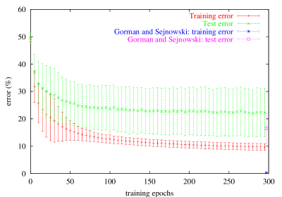
Figure 5: Learning curves for the sonar classification problem.

Gorman and Sejnowski [13] investigated the performance of sigmoidal neural networks on this data. Although the networks they used were quite different (since they involved deterministic units with real-valued outputs), the training error and test error they reported for a network with 6 hidden units is also illustrated in Figure 5.

6.2 Controlling an inverted pendulum

We also considered a problem of learning to balance an inverted pendulum. Figure 6 shows the arrangement: a puck moves in a square region. On the top of the puck is a weightless rod with a weight at its tip. The puck has no internal dynamics.

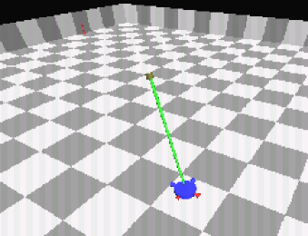
Figure 6: The inverted pendulum.

We investigated the performance of Algorithm 1 on this problem. We used a network with four hidden units, each receiving real numbers representing the position and velocity of the puck and the angle and angular velocity of the pendulum. These units were connected to two more units, whose outputs were used to control the sign of two 10N thrusts applied to the puck in the two axis directions. The reward signal was $0$ when the pendulum was upright, and $-1$ when it hit the ground. Once the pendulum hit the ground, the puck was randomly located near the centre of the square with velocity zero, and the pendulum was reset to vertical with zero angular velocity.

In the simulation, the square was $5\times 5$ metres, the dynamics were simulated in discrete time, with time steps of $0.02$s, the puck bounced elastically off the walls, gravity was $9.8$ms^-2, the puck radius was $50$mm, the puck height was $0$, the puck mass was $1$kg, air resistance was neglected, the pendulum length was $500$mm, the pendulum mass was $100$g, the coefficient of friction of the puck on the ground was $5\times 10^{-4}$, and friction at the pendulum joint was set to zero.

The algorithm parameters were $\gamma=10^{-6}$ and $\beta=0.995$.

Figure 7 shows a typical learning curve: the average time before the pendulum falls (in a simulation of $100000$ iterations $=2000$ seconds), as a function of total simulated time. Initial weights were chosen uniformly from the interval $(-0.05,0.05)$.

Figure 7: A typical learning curve for the inverted pendulum problem.

7 Further work

The most interesting questions raised by these results are concerned with possible biological mechanisms for update rules of this type. Some aspects of the update rule are supported by experimental results. Others, such as the reward signal, have not been investigated experimentally. One obvious direction for this work is the development of update rules for more realistic models of neurons. First, the model assumes discrete time. Second, it ignores some features that biological neurons are known to possess. For instance, the location of synapses in the dendritic tree allow timing relationships between action potentials in different presynaptic cells to affect the resulting postsynaptic potential. Other features of dendritic processing, such as nonlinearities, are also ignored by the model presented here. It is not clear which of these features are important for the computational properties of neural circuits.

8 Conclusions

The synaptic update rule presented in this paper requires only simple computations involving only local quantities plus a global reward signal. Furthermore, it adjusts the synaptic connection strengths to locally optimize the average reward received by the network. The reinforcement learning paradigm encompasses a considerable variety of learning problems. Simulations have shown the effectiveness of the algorithm for a simple pattern classification problem and an adaptive control problem.

References

- [1] A. G. Barto, C. W. Anderson, and R. S. Sutton. Synthesis of nonlinear control surfaces by a layered associative search network. Biological Cybernetics, 43:175–185, 1982.
- [2] A. G. Barto and R. S. Sutton. Landmark learning: An illustration of associative search. Biological Cybernetics, 42:1–8, 1981.
- [3] A. G. Barto, R. S. Sutton, and C. W. Anderson. Neuronlike adaptive elements that can solve difficult learning control problems. IEEE Transactions on Systems, Man, and Cybernetics, SMC-13:834–846, 1983.
- [4] A. G. Barto, R. S. Sutton, and P. S. Brouwer. Associative search network: A reinforcement learning associative memory. Biological Cybernetics, 40:201–211, 1981.
- [5] J. Baxter and P. L. Bartlett. On some algorithms for infinite-horizon policy-gradient estimation. Journal of Artificial Intelligence Research, 14, March 2001.
- [6] J. Baxter, P. L. Bartlett, and L. Weaver. Gradient-ascent algorithms and experiments with infinite-horizon, policy-gradient estimation. Journal of Artificial Intelligence Research, 14, March 2001.
- [7] T. V. Bliss and T. Lomo. Long-lasting potentiation of synaptic transmission in the dentate area of the anaesthetized rabbit following stimulation of the perforant path. Journal of Physiology (London), 232:331–356, 1973.
- [8] E. K. C. Blake and C. Merz. UCI repository of machine learning databases, 1998. http://www.ics.uci.edu/mlearn/MLRepository.html.
- [9] X.-R. Cao and H.-F. Chen. Perturbation Realization, Potentials, and Sensitivity Analysis of Markov Processes. IEEE Transactions on Automatic Control, 42:1382–1393, 1997.
- [10] X.-R. Cao and Y.-W. Wan. Algorithms for Sensitivity Analysis of Markov Chains Through Potentials and Perturbation Realization. IEEE Transactions on Control Systems Technology, 6:482–492, 1998.
- [11] G. A. Clark and E. R. Kandel. Induction of long-term facilitation in Aplysia sensory neurons by local application of serotonin to remote synapses. Proc. Natl. Acad. Sci. USA, 90:11411–11415, 1993.
- [12] T. L. Fine. Feedforward Neural Network Methodology. Springer, New York, 1999.
- [13] R. P. Gorman and T. J. Sejnowski. Analysis of hidden units in a layered network trained to classify sonar targets. Neural Networks, 1:75–89, 1988.
- [14] D. O. Hebb. The Organization of Behavior. Wiley, New York, 1949.
- [15] H. Kimura, K. Miyazaki, and S. Kobayashi. Reinforcement learning in POMDPs with function approximation. In D. H. Fisher, editor, Proceedings of the Fourteenth International Conference on Machine Learning (ICML’97), pages 152–160, 1997.
- [16] Y. Lo and M. ming Poo. Activity-dependent synaptic competition in vitro: Heterosynaptic suppression of developing synapses. Science, 254:1019–1022, 1991.
- [17] J. C. Magee and D. Johnston. A synaptically controlled, associative signal for Hebbian plasticity in hippocampal neurons. Science, 275:209–213, 1997.
- [18] P. Marbach and J. N. Tsitsiklis. Simulation-Based Optimization of Markov Reward Processes. Technical report, MIT, 1998.
- [19] H. Markram, J. Lübke, M. Frotscher, and B. Sakmann. Regulation of synaptic efficacy by coincidence of postsynaptic APs and EPSPs. Science, 275:213–215, 1997.
- [20] J. F. Medina and M. D. Mauk. Simulations of cerebellar motor learning: Computational analysis of plasticity at the mossy fiber to deep nucleus synapse. The Journal of Neuroscience, 19(16):7140–7151, 1999.
- [21] G. qiang Bi and M. ming Poo. Synaptic modifications in cultured hippocampal neurons: dependence on spike timing, synaptic strength, and postsynaptic cell type. The Journal of Neuroscience, 18(24):10464–10472, 1998.
- [22] D. Rumelhart, G. Hinton, and R. Williams. Learning representations by back-propagating errors. Nature, 323:533–536, 1986.
- [23] P. K. Stanton and T. J. Sejnowski. Associative long-term depression in the hippocampus induced by Hebbian covariance. Nature, 339:215–218, 1989.
- [24] G. J. Stuart and B. Sakmann. Active propagation of somatic action potentials into neocortical pyramidal cell dendrites. Nature, 367:69–72, 1994.
- [25] G. Tesauro. Simple neural models of classical conditioning. Biological Cybernetics, 55:187–200, 1986.
- [26] L. G. Valiant. Circuits of the mind. Oxford University Press, 1994.
- [27] R. J. Williams. Simple Statistical Gradient-Following Algorithms for Connectionist Reinforcement Learning. Machine Learning, 8:229–256, 1992.