Prototypical Networks for Multi-Label Learning

Abstract

We propose to formulate multi-label learning as a estimation of class distribution in a non-linear embedding space, where for each label, its positive data embeddings and negative data embeddings distribute compactly to form a positive component and negative component respectively, while the positive component and negative component are pushed away from each other. Duo to the shared embedding space for all labels, the distribution of embeddings preserves instances’ label membership and feature matrix, thus encodes the feature-label relation and nonlinear label dependency. Labels of a given instance are inferred in the embedding space by measuring the probabilities of its belongingness to the positive or negative components of each label. Specially, the probabilities are modeled as the distance from the given instance to representative positive or negative prototypes. Extensive experiments validate that the proposed solution can provide distinctively more accurate multi-label classification than other state-of-the-art algorithms.

Introduction

Multi-label learning addresses the problem that one instance can be associated with multiple labels simultaneously. Formally, the goal is to learn a function $F$, which maps an instance ${\bf{x}}\in\mathbb{R}^{D}$ to a label vector ${\bf{y}}=[l_{\_}{1},l_{\_}{2},\cdots,l_{\_}{K}]$ ($l_{\_}{i}$ is 1 if ${\bf{x}}$ is associated with the $i$-th label, and $l_{\_}{i}$ is 0 otherwise). Many real-world applications drive the study of this problem, such as image object recognition (Yang et al. 2016; Chen et al. 2019), text classification (Li, Ouyang, and Zhou 2015; Rubin et al. 2012), and bioinformatic problems (Yu et al. 2012).

How to exploit label dependency is the key to success in multi-label learning. Let ${\bf{X}}\in\mathbb{R}^{N\times D}$ denote all training instances, and ${\bf{Y}}\in\{0,1\}^{N\times K}$ be the corresponding label matrix. Previous research efforts study the label dependency mainly by 1) exploiting the label matrix Y only (Huang et al. 2018; Feng, An, and He 2019; Tai and Lin 2012; Zhang and Schneider 2012); and 2) jointly mapping X and Y into a same low rank label space (Guo 2017; Yu et al. 2014; Lin et al. 2014; Xu et al. 2014). The approaches using solely Y to extract label dependency only focus on how training instances carrying two different labels overlap with each other (which are the shared instances). They ignore the profiles of the shared instances (how they look like). Existing approaches using both X and Y often assume a low-rank linear structure of the label dependency. Simple and effective as it is, this assumption doesn’t necessarily hold in real world applications and oversimplifies the underlying complex label correlation patterns (Bhatia et al. 2015).

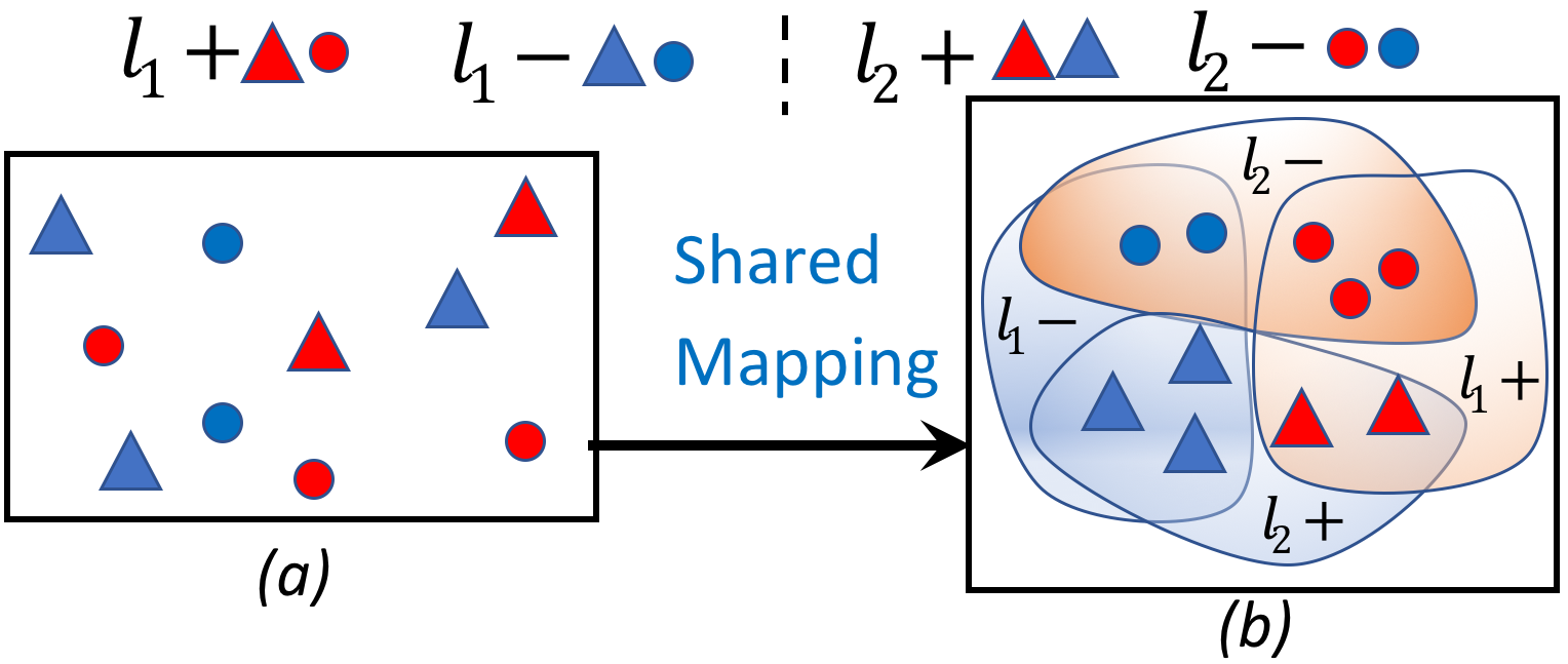
Figure 1: Intuition of our study: non-separable instances in the original feature space (a) are mapped to a non-linear embedding space (b) via feature embedding process applied to all labels. Label $l_{\_}1$ is indicated by color (red for positive and blue for negative). Label $l_{\_}2$ is presented by shape (triangle for positive and circle for negative). In space (b), ${l_{\_}k}+$/${l_{\_}k}-$ indicates the positive/negative component of label $k$, and data instances dropped into the area are tagged with both labels {$l_{\_}1$,$l_{\_}2$}, those in or only have {$l_{\_}1$} or {$l_{\_}2$} and those in carry neither of them. Label dependency is then captured by the distribution of instance embeddings in the new space.

Motivated by the previous research progress, we aim to exploit both X and Y to capture the non-linear label dependency. We attack the multi-label learning from a novel angle of distribution estimation. The intuition is that there exists an embedding space, in which for each label, its positive instances distribute compactly to form a positive component and the remained negative instances form a negative component, which is seperated as much as possible from the positive one. Figure 1 demonstrates the intuition. Instances are mapped into the embedding space described by Figure 1 (b), in which for each label $l_{\_}k(k=1,2)$, its positive instances are grouped into component ${l_{\_}k}+$, which is seperated from the negative component ${l_{\_}k}-$. The key to capture label dependency is the shared mapping function applied to all labels, without which (each label has its specific mapping function), classification for different labels will be done in different spaces independently and no label dependency will be exploited. Specially, by shared mapping, one embedding in the new space can adjust its position by its label membership and feature profile, which jointly exploits information from matrices X, Y and encodes non-linear label dependency into the distribution of embeddings.

We employ mixture density estimation to model the distribution of a positive/negative component and depending on the complexity of distributions, one positive/negative component can be represented by one or several clusters. We then define the mean of cluster as prototype and this comes the name of our approach PNML (Prototypical Networks for Multi-Label Learning). In practice, our PNML is proposed to work under two modes, named PNML-multiple and PNML-single. With mode PNML-multiple, the optimal number and parameters of prototypes are learned based on an adaptive clustering-like process, which brings us strong representation power for components at the sacrifice of computation efficiency. Mode PNML-single is thus proposed alternatively to compute one prototype for one component. For a given instance, its class membership to one label can be measured by its Bregman distance to the positive/negative prototypes of this label. The distance metric is learned for each label to model the different distribution pattern of each label. Specially, to exploit label dependency one more step, a designed label correlation regularizer is incorporated into the object function to carve these prototypes further.

We highlight our contributions as follows:

1. To the best of our knowledge, the proposed PNML method is the first attempt to address multi-label learning by jointly estimating the class distribution of all labels in an nonlinear embedding space, which exploiting non-linear label dependency and feature-label predicative relation effectively.

2. A Bregman divergence based distance metric is learned jointly for each label alongside with the mixing distribution model of the prototypes. It measures the closeness in distribution from a data instance to the positive and negative components of each label.

3. Extensive experiments including ablation study are conducted on 15 benchmark datasets. The results show the effectiveness of PNML, that PNML-multiple and PNML-single both achieve superior classification performance to all baselines.

Related Work

There have been many designs of various types of multi-label learning models. We concentrate on the discussion of the most recent and relevant work regarding the ways of exploiting label dependency.

Binary relevance based methods (R.Boutell et al. 2004) decompose a multi-label classification problem into $K$ independent binary classification problems while ignoring label dependency. It is known as the first-order approach. In contrast, methods in (Huang et al. 2018; Cai et al. 2013) make use of the pair-wise label co-occurrence pattern, and are thus featured as the second-order methods. For example, in JFSC (Huang et al. 2018), a pair-wise label correlation matrix ${\bf{C}}$ is calculated from $\bf{Y}$ and used to regularize the multi-label learning objective. RAKEL (Tsoumakas and Vlahavas 2007) exploits higher-order label dependency from ${\bf{Y}}$ by grouping labels as mutually exclusive meta-labels, so as to transform a multi-label classification task as a multi-class problem w.r.t. the meta-labels. CAMEL (Feng, An, and He 2019) learns to represent any given label as a linear combination of all the labels of Y. Among above approaches, JFSC (Huang et al. 2018) and CAMEL achieved state-of-the-art performance. Other methods (Tai and Lin 2012; Zhang and Schneider 2012; Guo 2017; Lin et al. 2014; Xu et al. 2014) exploit high-order label dependency by learning a low-rank representation of Y and a predicative mapping function between X and the low-rank label embedding. These two steps are conducted independently or jointly in these approaches. Nevertheless, the main limit of these methods is the low-rank assumption of the label matrix, which doesn’t necessarily hold in practices (Bhatia et al. 2015). Besides, the label dependency usually has a more complicated structure than the simple linear model.

MT-LMNN (Parameswaran and Weinberger 2010) and LM-kNN (Liu and Tsang 2015) also exploits both $\bf{X}$ and $\bf{Y}$ to extract the label dependency from the angle of metric learning. MT-LMNN treats the classification of each label as an individual task and a distance metric is learned for this label to keep an instance with this label stay closer to its neighbors also with this label. LM-kNN maps one instance’s feature profile and label vector onto a low dimensional manifold, where the projection of the feature and labels stay close to each other. Our approach can be also interpreted as a metric learning process, where an instance carrying or not a specific label $k$ is supposed to be close to the positive or negative prototypes of the label. Compared to MT-LMNN and LM-kNN, we jointly learn the prototypes and the distance metric of each label in the non-linear embedding space. Our approach is designed to be more flexible to capture the label dependency and the feature-label relation.

Our method is inspired by prototypical networks (Snell, Swersky, and Zemel 2017; Allen et al. 2019), which is originally designed for few-shot multi-class tasks. While the prototypes of different classes in the multi-class problem are loosely correlated. In our study, the positive and negative prototypes of different labels are strongly correlated. Such label correlation is captured by learning the self-tuning mixture distribution of each label. Besides, we learn the Bregman divergence function jointly to measure the similarity between a data instance and the prototypes, which adapts better to the data distribution than the primitive Euclidean distance used in (Snell, Swersky, and Zemel 2017; Allen et al. 2019).

Methodology

Overview of the Proposed Model

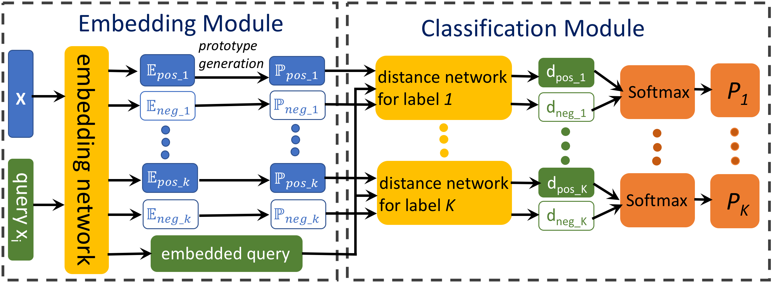
Figure 2: Overview of the proposed model PNML. For $k$=$1,...,K$, ${{\mathbb{E}}}_{\_}{{pos}\_k}$ (${\mathbb{E}}_{\_}{{neg}\_k}$) is the set of embeddings of positive (negative) instances for label $k$, i.e., $\mathbb{E}_{\_}{{pos}\_k}=\{{f_{\_}\phi}({\bf{x}}),{\bf{x}}\in{\mathbb{X}_{\_}{pos\_k}}\}$, where ${\mathbb{X}_{\_}{pos\_k}}$ is the positive instance set of label $k$. ${\mathbb{P}}_{\_}{{pos}\_k}$/${\mathbb{P}}_{\_}{{neg}\_k}$ is the positive/negative prototype set of label $k$. $d_{\_}{pos\_k}$/$d_{\_}{neg\_k}$ is the average distance from embedding of query ${{\bf{x}}_{\_}{\bf{i}}}$ to ${\mathbb{P}}_{\_}{{pos}\_k}$/${\mathbb{P}}_{\_}{{neg}\_k}$. $P_{\_}k$ is the predicted probability of ${{\bf{x}}_{\_}{\bf{i}}}$ having label $k$.

Figure 2 shows the overall architecture of PNML. In the training stage, the embedding module learns the non-linear feature embedding function applied to all the labels ${f_{\_}\phi}:{\mathbb{R}^{D}}\to{\mathbb{R}^{M}}$. Specially, this shared embedding function $f_{\_}\phi$ locates embedding in the new space by its label membership and original feature profile, which naturally encodes the information from label matrix ${\bf{Y}}$ and feature matrix ${\bf{X}}$ into the distribution of embeddings in the new space, and thus captures the non-linear label dependency. In Figure 2, the Embedding Layer network $f_{\_}\phi$ is defined by a one-layer fully connected neural network with LeakyRelu (Maas, Hannun, and Ng 2013) as activation function. In the new embedding space, the distribution of data instances of each label $k$ is described as a mixture of local prototypes ${\mathbb{P}}_{\_}{{pos}\_k}$ and ${\mathbb{P}}_{\_}{{neg}\_k}$ of positive and negative components $\mathbb{E}_{\_}{{pos}\_k}$ and $\mathbb{E}_{\_}{{neg}\_k}$. $\mathbb{E}_{\_}{{pos}\_k}=\{{f_{\_}\phi}({\bf{x}}),{\bf{x}}\in{\mathbb{X}_{\_}{pos\_k}}\}$, where ${\mathbb{X}_{\_}{pos\_k}}$ is the positive instance set of label $k$ and vice versa. With respect to the different strategies of prototype generation, PNML is proposed to work under two different modes, mode PNML-multiple and mode PNML-single:

• PNML-multiple: In this mode, prototypes in ${\mathbb{P}}_{\_}{{pos}\_k}$ and ${\mathbb{P}}_{\_}{{neg}\_k}$ are generated by an adaptive distance-based clustering-like process, in which the number and parameters of prototypes are tuned jointly in the training process. Usually multiple prototypes are generated in this adaptive process, so we call this mode PNML-multiple.

• PNML-single: In this mode, one prototype for one component is computed as the expectation of positive or negative embeddings of each label, so we call this mode PNML-single.

Mode PNML-multiple prefers more precise representation of components $\mathbb{E}_{\_}{{pos}\_k}$ and $\mathbb{E}_{\_}{{neg}\_k}$ compared to mode PNML-single, while its adaptive prototype generation process pays much computation efficiency. Alternatively, PNML-single is reduced to compute one prototype for one component, which saves computation significantly without much classification accuracy loss. We will introduce the prototype generation methods in these two modes next part and compare the two modes’ performance (classification accuracy and run time) in experiment part.

The classification module learns a Bregman-divergence based distance function for every label, based on the prototypes ${\mathbb{P}}_{\_}{{pos}\_k}$ and ${\mathbb{P}}_{\_}{{neg}\_k}$. In the testing stage, a query ${\bf x}_{\_}i$ is classified by going through the learned embedding layer to first have an embedding of ${\bf x}_{\_}i$. For each label, the distance between the embedding vector and each of the positive and negative prototypes is computed with the learned distance metric layer. These distance measurements actually represent the probabilities of ${\bf x}_{\_}i$’s belongingness to each cluster (one cluster is described by one prototype). softmax is then performed on these probabilities to determine whether ${\bf x}_{\_}i$ carries the label. We elaborate the design of PNML in the followings.

Mixture Density Estimation

Let ${\bf{e}}=f_{\_}\phi({\bf x})$ be the embedding vector of ${\bf x}$ in the embedding space. We assume that the class-conditional probability $p(\mathbf{e}|\hat{y}_{\_}{e}=\pm{1})$ of $\bf{e}$ belonging to positive or negative class of each label $k$ follows a mixture of the distributions of multiple positive or negative clusters, noted as $p(\left.{\bf{e}}\right|\boldsymbol{\Omega}^{+/-})$:

$$\begin{array}[]{c}p(\mathbf{e}|\hat{y}_{\_}{e}=\pm{1})=p(\left.{\bf{e}}\right|\boldsymbol{\Omega}^{+/-})=\sum\limits_{\_}{s=1}^{k_{\_}{+/-}}{{\pi^{+/-}_{\_}s}}{p_{\_}\psi}({\bf{e}}|{\boldsymbol{\theta}^{+/-}_{\_}s})\end{array}$$ (1)

where $\Omega^{+/-}=\{\pi^{+/-}_{\_}{s},\boldsymbol{\theta}^{+/-}_{\_}{s}\}$ are the learnable mixing coefficient and density function parameters of the mixture models of the positive and negative class. $k_{\_}{+/-}$ denotes the number of positive or negative clusters, which is tuned jointly in the training process in mode PNML-multiple and is set to 1 in mode PNML-single . For the convenience of analysis, we constrain each ${p_{\_}\psi}({\bf{e|}}\boldsymbol{\theta}^{+/-}_{\_}{s})$ to be an exponential family distribution function, with canonical parameters $\boldsymbol{\theta}^{+/-}_{\_}{s}$:

$$\begin{array}[]{r}{p_{\_}\psi}({\bf{e|}}\boldsymbol{\theta}^{+/-}_{\_}{s})=h(\mathbf{e})\exp(T({{\bf{e}}})\boldsymbol{\theta}^{+/-}_{\_}{s}-\psi(\boldsymbol{\theta}^{+/-}_{\_}{s}))\end{array}$$ (2)

where $T(\mathbf{e})$ denotes sufficient statistics of the distribution of $\mathbf{e}$ and $\psi(\boldsymbol{\theta}^{+/-}_{\_}{s})$ is the cumulant generating function, defined as the logarithm of the normalization factor to generate a proper probabilistic measure. $h(\mathbf{e})$ is the carrier measure.

Given learned $\boldsymbol{\Omega}^{+/-}$, we measure the posterior probability of $\bf{e}$ belonging to positive or negative class of each label as:

$$p({{\hat{y}}_{\_}{e}=+1}|{\bf{e}})=\frac{p(\left.{\bf{e}}\right|\boldsymbol{\Omega}^{+})}{p(\left.{\bf{e}}\right|\boldsymbol{\Omega}^{+})+p(\left.{\bf{e}}\right|\boldsymbol{\Omega}^{-})}$$ (3)

where the positive and negative class prior probabilities are set equally as $0.5$. Without specified prior domain knowledge, the non-informative prior is a reasonable choice. Eq. (3) can be thus interpreted as a likelihood ratio test.

According to the Theorem 4 in (Banerjee et al. 2005), there is a unique Bregman divergence associated with every member of the exponential family. For example, spherical Gaussian distribution is associated with squared Euclidean distance Therefore, we can rewrite the regular exponential family distribution given in Eq.(2) by a regular Bregman divergence (Snell, Swersky, and Zemel 2017; Banerjee et al. 2005) as:

$$\begin{array}[]{r}{p_{\_}\psi}({\bf{e|}}\boldsymbol{\theta}^{+/-}_{\_}{s})=\exp(-{d_{\_}\varphi}({\bf{e}},\mu(\boldsymbol{\theta}^{+/-}_{\_}{s}))-{g_{\_}\varphi}({\bf{e}}))\end{array}$$ (4)

where $d_{\_}\varphi$ is the unique Bregman divergence determined by the conjugate Legendre function of $\psi$. $g_{\_}{\psi}(\mathbf{e})$ absorbs all the rest terms that are not related to $\mathbf{e}$, but determined by $\psi$. $\mu(\boldsymbol{\theta})$ is the expectation of the exponential family distribution defined by Equation (5).

$$\begin{array}[]{r}\mu(\boldsymbol{\theta})=E_{\_}{p_{\_}\psi}[{\bf{e}}]=\int_{\_}{\mathbb{R}^{M}}{{\bf{e}}{p_{\_}\psi}({\bf{e|}}\boldsymbol{\theta})d{\bf{e}}}\end{array}$$ (5)

Prototype Generation for Mode PNML-single.   We define the expectation in Equation (5) as prototype. In mode PNML-single, one positive/negative component of label $k$ is treated as one positive/negative cluster, so one positive/negative prototype is computed for it as:

$${{\bf{P}}_{\_}{pos\_k/neg\_k}}=\frac{1}{{\left|{{{\mathbb{X}}_{\_}{pos\_k/neg\_k}}}\right|}}\sum\limits_{\_}{{{\bf{x}}_{\_}i}\in{{\mathbb{X}}_{\_}{pos\_k/neg\_k}}}{{f_{\_}\phi}({{\bf{x}}_{\_}i})}$$ (6)

where $\left|{{{\mathbb{X}}_{\_}{pos\_k/neg\_k}}}\right|$ is the size of set ${{{\mathbb{X}}_{\_}{pos\_k/neg\_k}}}$. Here ${{\bf{P}}_{\_}{pos\_k}}$ composes the positive prototype set ${{\mathbb{P}}_{\_}{pos\_k}}$ and ${{\bf{P}}_{\_}{neg\_k}}$ composes the negative prototype set ${{\mathbb{P}}_{\_}{neg\_k}}$.

Prototype Generation for Mode PNML-multiple.   We adopt an adaptive process in mode PNML-multiple to generate prototype based on real-world data’s statistical profiles. In our study, without loss of generality, we concretize the distribution of each prototype described by Equation (2). The Bregman divergence of each positive or negative prototype $d_{\_}{\psi}(\mathbf{e},\mu(\boldsymbol{\theta}^{+/-}_{\_}{s}))$ is thus can be used to evaluate the probability of $\mathbf{e}$’s belongingness to each prototype. To learn these prototypes, we follow the idea of infinite mixture distribution applied previously in (Kulis and Jordan 2012; Allen et al. 2019). The main steps are :

1. Initialize ${\boldsymbol{\mu}_{\_}c}$ = $\mu_{\_}{\mathbb{E}_{\_}{{pos}\_k}}$ ($\mu_{\_}{\mathbb{E}_{\_}{{neg}\_k}}$) as the mean of ${\mathbb{E}}_{\_}{{pos}\_k}$ (${\mathbb{E}}_{\_}{{neg}\_k}$), $C=1$ as the initial number of prototypes, and ${\sigma_{\_}c}=\sigma$ , which is the trainable variance of one cluster from which instance is assumed to be sampled. ite_clustering is the iteration number of clustering.

2. Estimate the distance threshold (Eq.7) for creating a new prototype:

   $$\lambda=-2\sigma\log\left({\frac{\alpha}{{{{(1+\frac{\rho}{\sigma})}^{M/2}}}}}\right)$$ (7)

   where $\rho$ is a measure of the standard deviation for the base distribution from which prototypes are drawn, $M$ is the dimension of embedding vector and $\alpha$ is a hyperparameter named concentration parameter.

3. For each embedding vector $\mathbf{e}_{\_}i$ in ${\mathbb{E}}_{\_}{{pos}\_k}$ (${\mathbb{E}}_{\_}{{neg}\_k}$), compute its’ distance to each prototype $c$ in $\{1,\cdots,C\}$ as ${d_{\_}{i,c}}={d_{\_}\psi}({{\bf{e}}_{\_}{\bf{i}}}{\bf{,}}{\boldsymbol{\mu}_{\_}{\bf{c}}}).$ If ${\min_{\_}c}{d_{\_}{i,c}}>\lambda$ , set $C=C+1$, update $\boldsymbol{\mu}_{\_}c={\mathbf{e}_{\_}i}$ and ${\sigma_{\_}c}={\sigma}$. After that, compute the probability of $\mathbf{e}_{\_}i$ belonging to each cluster by ${z_{\_}{i,c}}=\frac{{\exp(-{d_{\_}\varphi}({\mathbf{e}_{\_}i},{\boldsymbol{\mu}_{\_}c}))}}{{\sum\nolimits_{\_}c{\exp(-{d_{\_}\varphi}({\mathbf{e}_{\_}i},{\boldsymbol{\mu}_{\_}c}))}}}$ , and then recompute the cluster mean as ${\boldsymbol{\mu}_{\_}c}=\frac{{\sum\nolimits_{\_}i{{z_{\_}{i,c}}}{\mathbf{e}_{\_}i}}}{{\sum\nolimits_{\_}i{{z_{\_}{i,c}}}}}$.

4. Repeat step 3 for ite_clustering times. Finally, Each $\boldsymbol{\mu}_{\_}c$ is a prototype vector and all $\boldsymbol{\mu}_{\_}c$, $c=1,...,C$ compose the prototype set ${\mathbb{P}}_{\_}{{pos}\_k}$ (${\mathbb{P}}_{\_}{{neg}\_k}$).

With the defination of prototype, combining Equation (1), (3) and (4) and adopting noninformative class and cluster prior probability, we can write the prediction probability of query ${{\bf{x}}_{\_}{\bf{i}}}$’s having label $k$ as:

where $\left|{{{\mathbb{P}}_{\_}{{pos\_k}/{neg\_k}}}}\right|$ is the size of positive/negative prototype set of label $k$. ${{\bf{P}}_{\_}{{pos\_k\_c}/{neg\_k\_c}}}$ is the $c$-th prototype vector in ${{{\mathbb{P}}_{\_}{{pos\_k}/{neg\_k}}}}$.

Based on Equation 8, we can formulate the learning objective function of PNML as a cross-entropy loss:

$$\begin{array}[]{*{20}{c}}{{L_{\_}e}=-\sum\limits_{\_}{i=1}^{N}{\sum\limits_{\_}{k=1}^{K}{{y_{\_}{i,k}}\log p(}{{\hat{y}}_{\_}{i,k}}=+1|{{\bf{x}}_{\_}i})}}\\ {+(1-{y_{\_}{i,k}})\log(1-p({{\hat{y}}_{\_}{i,k}}=+1|{{\bf{x}}_{\_}i}))}\end{array}$$ (9)

We next move to the second module of distance metric learning for classification.

Label-Wise Distance Metric Learning

In (Banerjee et al. 2005), various distance functions $d_{\_}\varphi(\cdot,\cdot)$ are presented for popular distribution functions in exponential families. For example, multivariate spherical Gaussian distribution ${p_{\_}\psi}({\bf e|\boldsymbol{\theta}})$ is associated with squared Euclidean distance $||{\bf{e}}-\mu(\boldsymbol{\theta})||^{2}$. Although Euclidean distance is simple and showed its effectiveness in (Snell, Swersky, and Zemel 2017), it is not appropriate to our multi-label learning, because components of our label distribution may not be spherical Gaussian distribution.

The non-spherical distribution can be firstly caused by the instances’ common membership among different categories. One component may be pulled to get close to several different components due to their common instances. Secondly, for multi-label learning, features may play different roles in different labels’ discriminant processes (Zhang 2011; Huang et al. 2018), which implies that each label has its own specific distribution pattern.

We are therefore encouraged to learn approximating the Bregman divergence $d_{\_}{\psi}(\mathbf{e},\boldsymbol{\mu}(\theta_{\_}{s}))$ for each label by learning a Mahalanobis distance function ${d_{\_}m^{k}}$ given the mean vector of the prototypes in the embedding space, which shows:

$${d_{\_}m^{k}}({{\bf{e}}},{{\boldsymbol{\mu}_{\_}{s}}})=\sqrt{({{\bf{e}}-{\boldsymbol{\mu}_{\_}{s}})^{T}}{{\mathbf{U}_{\_}k}^{T}}{\mathbf{U}_{\_}k}({\bf{e}}-{\boldsymbol{\mu}}_{\_}{s})}$$ (10)

The non-spherical covariance structure is approximated by the weight matrix $\mathbf{U}_{\_}{k}\in{\mathbb{R}^{M\times{M}}}$ learned from the data (Weinberger and Saul 2009; Parameswaran and Weinberger 2010).

In this paper, we encode $\bf{U_{\_}k}$ with a one-layer fully connected neural network with a linear activation function, as shown in Distance Network in Figure 2. Eq. (9). Moreover, we add a regularizer described by Equation (11) to the overall loss function to prevent over-fitting of the distance metric learning.

$${L_{\_}m}=\sum_{\_}{k=1}^{K}\left\|{\bf{U}_{\_}k}\right\|_{\_}F^{2}$$ (11)

Label Correlation Regularizer

In our approach, the prototypes can be viewed as labels’ representatives, especially the positive prototypes. In practice, the negative instances for a label are usually much more than the corresponding positive instances. Then for many labels, their negative instances are mostly in common. Consequently the negative prototypes of labels may be similar, and less interesting than positive prototypes. We thus take the positive prototypes and enhance the correlation between positive prototypes of different labels in the training process. Intuitively, if label $j$ and $k$ are positively correlated in $\bf{Y}$, the mean of their positive prototypes should be close as well and thus present a large inner product. We introduce an regularization term defined by:

$${L_{\_}c}=\frac{1}{2}\sum\limits_{\_}{j=1}^{K}{\sum\limits_{\_}{k=1}^{K}{(1-{c_{\_}{jk}})\mu{{({{\mathbb{P}}_{\_}{pos\_j}})}^{T}}\mu({{\mathbb{P}}_{\_}{pos\_k}})}}$$ (12)

where $c_{\_}{jk}$ indicates the correlation measurement between $j$-th column and $k$-th column of label matrix $\bf Y$. ${\mu({{\mathbb{P}}_{\_}{pos\_j}})}$ and ${\mu({{\mathbb{P}}_{\_}{pos\_k}})}$ are the mean vector of prototype set ${{{\mathbb{P}}_{\_}{pos\_j}}}$ and ${{{\mathbb{P}}_{\_}{pos\_k}}}$.

The overall loss function is given in Eq. (13), where $\lambda_{\_}1$ and $\lambda_{\_}2$ are the non-negative tradeoff parameters.

$${L_{\_}{all}}={L_{\_}e}+{\lambda_{\_}1}{L_{\_}m}+{\lambda_{\_}2}{L_{\_}c}$$ (13)

Training procedure

In the training process of our approach, for each label, we need to load the feature matrix $\bf{X}$ for mapping and building prototypes. In mode PNML-single, the mean of embedding set $\mathbb{E}_{\_}{{pos}\_k}$ and $\mathbb{E}_{\_}{{neg}\_k}$ needs to be computed during every training iteration, and in mode PNML-multiple, distance from every instance embedding ${{\bf{e}}_{\_}i}$ to cluster centroids needs to be compared to threshold. The computational cost significantly increases when data sets get larger. To mitigate this issue, we can sample instances for each label to reduce the amount of data involved for prototype computing. We denote ${r_{\_}{pos\_k}}$ and ${r_{\_}{neg\_k}}$ as the sampling rate for positive and negative instances, respectively. Usually, compared to ${r_{\_}{neg\_k}}$, ${r_{\_}{pos\_k}}$ is set bigger to sample as many positive instances as possible since they are more informative and rare, while ${r_{\_}{neg\_k}}$ is set smaller to reduce computation significantly without losing much information. The influence of the sampling rate on model performance will be evaluated in next section.

The training procedure first samples positive and negative instances respectively. Then the network weights for embedding ${f_{\_}\phi}$, distance metric $d_{\_}m^{k}(\cdot,\cdot)$ and the prototypes’ parameters are updated. Adam (Kingma and Ba 2015) is used as the optimizer.

Experiments

We organised comprehensive experiments in this section. Due to the limited space, we intorducte the implementation platforms in supplementary document, also further experimental results.

Experimental Setup

Datasets and Evaluation Metrics.   Fifteen public benchmark datasets are used to evaluate all the involved approaches comprehensively. These datasets have different application contexts, including text, biology, music and image. Table 1 summarizes the details of these data sets. We choose $5$ popularly applied evaluation metrics to measure the performances (Sorower 2010). They are Accuracy, Macro-averaging $F_{\_}{1}$, Micro-averaging $F_{\_}{1}$, Average  precision and Ranking  Loss.

Table 1: Used benchmark multi-label datasets. $N$/$D$ denotes the number of instances/features of a data set. $Labels$ denotes the number of label in dataset. $Card$ denotes the average number of labels associated with each instance.

dataset	$N$	$D$	$Labels$	$Card$	domain
emotions	593	72	6	1.869	music
scene	2407	294	5	1.074	image
image	2000	294	5	1.240	image
arts	5000	462	26	1.636	text(web)
science	5000	743	40	1.451	text(web)
education	5000	550	33	1.461	text(web)
enron	1702	1001	53	3.378	text
genbase	662	1186	27	1.252	biology
rcv1-s1	6000	944	101	2.880	text
rcv1-s3	6000	944	101	2.614	text
rcv1-s5	6000	944	101	2.642	text
bibtex	7395	1836	159	2.402	text
corel5k	5000	499	374	3.522	image
bookmark	87856	2150	208	2.028	text
imdb	120919	1001	28	2.000	text

Comparing Approaches.   We compare PNML with the following 6 multi-label learning approaches, including first-order, second-order and high-order approaches. Some of these approaches achieve state-of-the-art multi-label classification performance and half of them were proposed within 3 years. Specially, an state-of-the-art extreme multi-lable classification approach is also introduced for broder comparison. The comparing approaches are:

• BR (R.Boutell et al. 2004): It decomposes multi-label problem as $K$ independent single-label classification problems and is a first-order approach

• ML-KNN (Zhang and Zhou 2007): It is derived from traditional KNN method for multi-label problem and it is a high-order approach.

• MLTSVM (Chen et al. 2016): It is adapted from SVM.

• JFSC (Huang et al. 2018): It does feature selection and classification for each label jointly. It is a second-order approach and is one of the state-of-the-art approach.

• CAMEL (Feng, An, and He 2019): It treats each label as a linear combination of all other labels. It is a high-order approach and is one of the state-of-the-art approach.

• Parabel (Prabhu et al. 2018):It is one of the state-of-the-art multi-label extreme classification methods. Since Parabel is designed specially for ranking, so to keep fairness, we just compare their performance in terms of the ranking metrics, that is Ranking  Loss and Average  precision.

Baseline models of BR, ML-KNN and MLTSVM are implemented with the scikit-learn package (Szymański and Kajdanowicz 2017) and a two-layer multi-layer perceptron is used as the base classifier for BR. The unit number of hidden layer of MLP is determined by Eq.(14) where $D$ is the input feature dimension. Besides, the number of nearest neighbors of ML-KNN is searched in $\{3,5,\cdots,21\}$. For MLTSVM, the empirical risk penalty parameter $c_{\_}k$ and regularization parameter ${\lambda_{\_}k}$ are searched in $\{{2^{-6}},{2^{-5}},{2^{-4}},\cdots,{2^{4}}\}$. Codes and suggested parameters in the original papers are used for JFSC, CAMEL and Parabel.

In our approach, the embedding dimension $M$, slope of LeakyRelu $\beta$, concentration parameter $\alpha$ (only needed by PNML-multiple mode) and loss tradeoff parameters $\lambda_{\_}1$, $\lambda_{\_}2$ are hyperparameters to be determined. Empirically, $\beta$ is set to $0.2$ and $M$ is determined by Eq.(14), in which $D$ is the feature dimension in original feature space. $\lambda_{\_}1$ and $\lambda_{\_}2$, they are searched in $\{{10^{-7}},5\times{10^{-6}},{10^{-6}},5\times{10^{-6}},\cdots,{10^{-2}}\}$. When under mode PNML-multiple, $\alpha$ is searched in $\{0.0001,0.001,0.01,0.1,0.5,1.0\}$.

$$M=\left\{{\begin{array}[]{*{20}{c}}{72}\\ {128}\end{array}\begin{array}[]{*{20}{c}}{D\leq 200}\\ {D>200}\end{array}}\right.$$ (14)

Classification Results

Table 2: Experimental results of evaluated algorithms on 15 data sets on 5 evaluation metrics. $\uparrow\left(\downarrow\right)$ indicates the larger (smaller) the value, the better the performance. The best results are in bold . AR is the average rank of algorithm on 15 data sets with corresponding metric.

Comparing	$Accuracy$ $\uparrow$
Algorithm	emotions	scene	image	arts	science	education	enron	genbase	rcv1-s1	rcv1-s3	rcv1-s5	bibtex	corel5k	bookmark	imdb	AR
BR	0.478	0.672	0.530	0.341	0.350	0.365	0.419	0.988	0.324	0.378	0.381	0.321	0.106	0.233	0.065	4.47
ML-KNN	0.418	0.692	0.522	0.189	0.280	0.324	0.273	0.973	0.338	0.342	0.349	0.313	0.079	0.242	0.145	5.27
MLTSVM	0.320	0.418	0.500	0.241	0.309	0.283	0.273	0.952	0.235	0.245	0.312	0.201	0.091	0.173	0.071	6.47
JFSC	0.255	0.603	0.451	0.377	0.365	0.346	0.418	0.994	0.354	0.391	0.397	0.352	0.142	0.250	0.248	3.60
CAMEL	0.505	0.702	0.589	0.342	0.331	0.360	0.440	0.992	0.300	0.354	0.358	0.312	0.079	0.239	0.098	4.20
Parabel	–	–	–	–	–	–	–	–	–	–	–	–	–	–	–	–
PNML-single	0.489	0.708	0.583	0.381	0.394	0.394	0.472	0.987	0.395	0.422	0.428	0.387	0.121	0.253	0.109	2.53
PNML-multiple	0.509	0.728	0.603	0.393	0.402	0.400	0.475	0.990	0.398	0.427	0.431	0.390	0.123	0.258	0.121	1.33
Comparing	$Micro-averaging\ \ F_{\_}{1}$ $\uparrow$
Algorithm	emotions	scene	image	arts	science	education	enron	genbase	rcv1-s1	rcv1-s3	rcv1-s5	bibtex	corel5k	bookmark	imdb	AR
BR	0.609	0.735	0.615	0.400	0.410	0.442	0.540	0.990	0.426	0.435	0.449	0.426	0.185	0.244	0.105	4.73
ML-KNN	0.548	0.748	0.592	0.250	0.348	0.403	0.425	0.979	0.426	0.394	0.413	0.416	0.143	0.317	0.180	5.33
MLTSVM	0.484	0.559	0.560	0.319	0.376	0.376	0.436	0.963	0.379	0.362	0.453	0.340	0.160	0.226	0.137	6.27
JFSC	0.407	0.697	0.552	0.444	0.446	0.445	0.542	0.994	0.495	0.487	0.497	0.471	0.243	0.281	0.342	3.33
CAMEL	0.636	0.770	0.659	0.409	0.421	0.450	0.564	0.993	0.403	0.413	0.431	0.421	0.110	0.278	0.166	3.87
Parabel	–	–	–	–	–	–	–	–	–	–	–	–	–	–	–	–
PNML-single	0.630	0.744	0.648	0.440	0.454	0.471	0.596	0.988	0.533	0.516	0.532	0.501	0.198	0.262	0.194	2.87
PNML-multiple	0.648	0.757	0.662	0.446	0.462	0.474	0.598	0.991	0.534	0.518	0.540	0.502	0.207	0.268	0.203	1.53
Comparing	$Macro-averaging\ \ F_{\_}{1}$ $\uparrow$
Algorithm	emotions	scene	image	arts	science	education	enron	genbase	rcv1-s1	rcv1-s3	rcv1-s5	bibtex	corel5k	bookmark	imdb	AR
BR	0.578	0.746	0.612	0.245	0.241	0.221	0.231	0.747	0.271	0.244	0.244	0.311	0.041	0.173	0.049	3.47
ML-KNN	0.528	0.755	0.589	0.146	0.169	0.176	0.140	0.674	0.239	0.184	0.208	0.267	0.027	0.191	0.040	5.33
MLTSVM	0.479	0.570	0.564	0.200	0.173	0.156	0.127	0.600	0.201	0.162	0.135	0.205	0.036	0.104	0.032	6.40
JFSC	0.352	0.701	0.546	0.235	0.222	0.144	0.196	0.746	0.256	0.225	0.232	0.354	0.039	0.136	0.080	4.80
CAMEL	0.619	0.779	0.662	0.232	0.206	0.198	0.212	0.755	0.177	0.156	0.156	0.251	0.026	0.139	0.087	4.40
Parabel	–	–	–	–	–	–	–	–	–	–	–	–	–	–	–	–
PNML-single	0.634	0.756	0.655	0.328	0.296	0.310	0.258	0.746	0.378	0.365	0.372	0.418	0.064	0.232	0.156	1.87
PNML-multiple	0.647	0.767	0.666	0.321	0.298	0.304	0.262	0.733	0.389	0.375	0.377	0.414	0.066	0.228	0.144	1.67
Comparing	$Average\ \ precision$ $\uparrow$
Algorithm	emotions	scene	image	arts	science	education	enron	genbase	rcv1-s1	rcv1-s3	rcv1-s5	bibtex	corel5k	bookmark	imdb	AR
BR	0.604	0.721	0.632	0.378	0.369	0.388	0.418	0.989	0.314	0.376	0.377	0.318	0.276	0.424	0.504	7.00
ML-KNN	0.652	0.824	0.682	0.380	0.410	0.453	0.521	0.982	0.537	0.541	0.558	0.348	0.218	0.299	0.399	6.93
MLTSVM	0.636	0.800	0.770	0.545	0.560	0.592	0.680	0.997	0.569	0.605	0.585	0.520	0.241	0.401	0.424	5.60
JFSC	0.720	0.851	0.788	0.604	0.592	0.626	0.641	0.997	0.600	0.619	0.630	0.594	0.292	0.441	0.496	3.87
CAMEL	0.783	0.893	0.825	0.596	0.604	0.621	0.678	0.997	0.604	0.633	0.631	0.606	0.293	0.463	0.479	2.80
Parabel	0.613	0.861	0.794	0.349	0.481	0.474	0.479	0.998	0.589	0.616	0.635	0.604	0.267	0.458	0.483	4.87
PNML-single	0.769	0.867	0.816	0.609	0.608	0.635	0.682	0.992	0.627	0.630	0.640	0.608	0.273	0.476	0.445	2.93
PNML-multiple	0.788	0.872	0.828	0.622	0.611	0.638	0.682	0.994	0.633	0.635	0.644	0.611	0.286	0.481	0.450	1.73
Comparing	$Ranking\ \ loss$ $\downarrow$
Algorithm	emotions	scene	image	arts	science	education	enron	genbase	rcv1-s1	rcv1-s3	rcv1-s5	bibtex	corel5k	bookmark	imdb	AR
BR	0.490	0.289	0.437	0.611	0.591	0.587	0.477	0.010	0.583	0.546	0.535	0.616	0.153	0.095	0.159	6.93
ML-KNN	0.308	0.101	0.257	0.192	0.135	0.104	0.111	0.012	0.067	0.067	0.061	0.160	0.134	0.187	0.218	5.73
MLTSVM	0.374	0.102	0.175	0.128	0.099	0.077	0.077	0.004	0.043	0.040	0.060	0.065	0.143	0.172	0.204	4.00
JFSC	0.242	0.090	0.176	0.162	0.151	0.104	0.130	0.002	0.065	0.065	0.064	0.081	0.178	0.146	0.167	4.80
CAMEL	0.183	0.065	0.150	0.170	0.140	0.135	0.103	0.003	0.073	0.069	0.063	0.095	0.225	0.101	0.189	4.87
Parabel	0.356	0.075	0.172	0.272	0.171	0.168	0.208	0.001	0.068	0.065	0.061	0.084	0.312	0.132	0.163	4.93
PNML-single	0.192	0.077	0.150	0.118	0.101	0.072	0.079	0.002	0.037	0.043	0.039	0.071	0.143	0.092	0.174	2.93
PNML-multiple	0.181	0.076	0.147	0.110	0.093	0.070	0.077	0.001	0.035	0.041	0.038	0.062	0.131	0.088	0.171	1.40

Table 3: Results of pairwise comparison applied to PNML-single (PNML-multiple) with baseline algorithms.

comparing algorithms	win	tie	lose	$\begin{array}[]{c}V/2+1.96\sqrt{V}/2\end{array}$	superior
BR	73	0	2	45.987 ($V=75$)	yes
ML-KNN	73	0	2		yes
MLTSVM	72	1	2		yes
JFSC	62	0	13		yes
CAMEL	59	0	16		yes
Parabel	24	1	5	20.368 ($V=30$)	yes

For each comparing approach, 5-fold cross-validation is performed on the training data of each data set. Tables 2 reports the average results of each comparing algorithm over 15 data sets in terms of each evaluation metric. Table 3 summarizes the overall pairwise comparison results by comparing PNML-single (PNML-multiple) with other baselines. Based on these experimental results, the following observations can be made.

• Our approach PNML-single (PNML-multiple) outperforms the baseline approaches in most cases. Concretely, if we treat one evaluation metric for one dataset as one case, there are 75 cases in total. PNML-single outperforms all the other baselines in 73% ($55/75$) evaluation cases, and PNML-multiple outperforms them in 73% ($55/75$) evaluation cases. Besides, the average rank of PNML-single and PNML-multiple is higher than all the other baselines with every evaluation metric. Moreover, in Table 3, pairwise comparison is done between PNML-single (PNML-multiple) and other baseline algorithms. Generally, we have $15\times 5=75$ cases, while for Parabel, we have $15\times 2=30$ cases. The sign test (Demsar 2006) is employed to test whether PNML-single (PNML-multiple) achieves a competitive performance against the other comparing algorithms. If the number of wins is at least $V/2+1.96\sqrt{V}/2$ ($V$ is the number of cases), the algorithm is significantly better with significance level $\alpha<0.05$. The results of indicate PNML-single (PNML-multiple) is significantly superior to other baselines.

• In terms of evaluation metric, PNML-single (PNML-multiple) performs best on Macro-averaging $F_{\_}{1}$, which indicates PNML-single (PNML-multiple) is more friendly to rarely encountered labels comparing to other approaches. This observation matches the results of (Snell, Swersky, and Zemel 2017), in which prototypical networks are used to solve few-shot learning problem.

• PNML-multiple outperforms PNML-single in most cases, which indicates the learned multiple prototypes can describe the embedding distribution more comprehensively than one prototype. While PNML-single is more efficient than PNML-multiple. See supplementary document for detailed run-time evaluation.

Ablation Study

Without loss of generality, we tune the architecture of our proposed approach to verify the effectiveness of different parts under mode PNML-multiple.

• To confirm that our approach can learn well the label dependency and perform an effective mapping ${f_{\_}\phi}$, we assign different independently trained embedding layers to each label. Therefore $K$ single-label classifications are conducted independently without interaction. We name this variant of the proposed approach as PNML-I.

• To demonstrate the effectiveness of the distance metric learning component, we build another variant of our approach in which Euclidean distance is used for each label and we name it PNML-D.

Table 4 summarizes the overall pairwise comparison results by comparing PNML-multiple with PNML-I and PNML-D. The superiored results verifies that the learned embedding function ${f_{\_}\phi}$ does transfer meaningful knowledge across labels, the learned label-specific distance metric achieves better distribution modelling than Euclidean. See supplementary document for detailed results.

Table 4: Results of pairwise comparison applied to PNML-multiple with PNML variants.

comparing algorithms	win	tie	lose	$\begin{array}[]{c}V/2+1.96\sqrt{V}/2\end{array}$	superior
PNML-I	68	1	6	45.987 ($V=75$)	yes
PNML-D	75	0	0		yes

Influence of Instance Sampling Rate

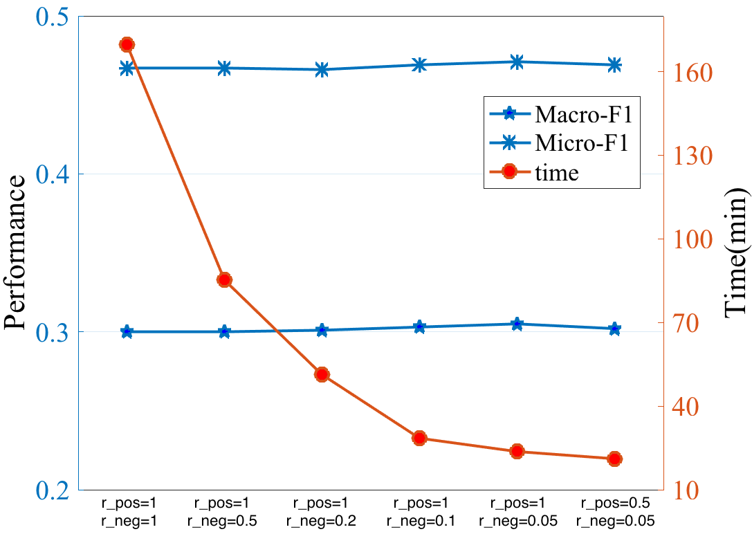
Figure 3: Performance and run-time under different sampling rates.

In our approach, to reduce the computational cost, we sample positive instances and negative instances for each label at rate $r_{\_}{pos\_k}$ and $r_{\_}{neg\_k}$ in the training process. Here, we show the influence of sampling rates on model predictive performance and efficiency. We choose dataset arts for the experimental study and record the change of Macro-averaging $F_{\_}{1}$, Micro-averaging $F_{\_}{1}$ and run-time of 5 folds under different sampling rates in Figure 3. Here PNML works under the mode PNML-single. It can be observed that the performance keeps nearly the same under different sampling rates, while run-time drops down with the decreasing of sampling rate.

Conclusion and Future Work

In this paper, we propose PNML to addresse multi-label learning by estimation of class distribution in a new embedding space. While assuming each label has a mixture distribution of two components, a mapping function is learned to map label-wise training instances to two compact clusters, one for each component. Then positive and negative prototypes are defined for each label based on the distribution of embeddings (mode PNML-multiple) or as the expectations of positive embeddings and negative embeddings (mode PNML-single). Our approach can be extended to weak label problem and positive unlabeled problem in the future.

Appendix A Further Experimental Results

Ablation Study

Table 5 gives the detailed results of ablation study.

Table 5: Experimental results of evaluated algorithms on 15 data sets on 5 evaluation metrics. $\uparrow\left(\downarrow\right)$ indicates the larger (smaller) the value, the better the performance. The best results are in bold . AR is the average rank of algorithm on 15 data sets with corresponding metric.

Comparing	$Accuracy$ $\uparrow$
Algorithm	emotions	scene	image	arts	science	education	enron	genbase	rcv1-s1	rcv1-s3	rcv1-s5	bibtex	corel5k	bookmark	imdb
PNML-I	0.492	0.697	0.572	0.364	0.351	0.385	0.420	0.987	0.352	0.384	0.397	0.356	0.121	0.221	0.108
PNML-D	0.415	0.669	0.556	0.361	0.366	0.386	0.430	0.974	0.366	0.387	0.389	0.307	0.109	0.198	0.089
PNML-multiple	0.519	0.728	0.603	0.393	0.402	0.400	0.475	0.990	0.398	0.427	0.431	0.390	0.123	0.258	0.121
Comparing	$Micro-averaging\ \ F_{\_}{1}$ $\uparrow$
Algorithm	emotions	scene	image	arts	science	education	enron	genbase	rcv1-s1	rcv1-s3	rcv1-s5	bibtex	corel5k	bookmark	imdb
PNML-I	0.628	0.751	0.642	0.417	0.407	0.450	0.540	0.989	0.470	0.453	0.475	0.452	0.190	0.239	0.191
PNML-D	0.552	0.711	0.623	0.421	0.425	0.460	0.556	0.974	0.501	0.478	0.499	0.411	0.174	0.214	0.183
PNML-multiple	0.653	0.757	0.662	0.446	0.462	0.474	0.598	0.991	0.534	0.518	0.540	0.502	0.207	0.268	0.203
Comparing	$Macro-averaging\ \ F_{\_}{1}$ $\uparrow$
Algorithm	emotions	scene	image	arts	science	education	enron	genbase	rcv1-s1	rcv1-s3	rcv1-s5	bibtex	corel5k	bookmark	imdb
PNML-I	0.641	0.762	0.642	0.288	0.240	0.255	0.242	0.737	0.343	0.280	0.294	0.348	0.061	0.224	0.146
PNML-D	0.554	0.739	0.633	0.313	0.282	0.280	0.253	0.719	0.367	0.353	0.354	0.375	0.058	0.209	0.137
PNML-multiple	0.652	0.767	0.666	0.328	0.298	0.311	0.262	0.733	0.389	0.375	0.377	0.420	0.066	0.228	0.144
Comparing	$Average\ \ precision$ $\uparrow$
Algorithm	emotions	scene	image	arts	science	education	enron	genbase	rcv1-s1	rcv1-s3	rcv1-s5	bibtex	corel5k	bookmark	imdb
PNML-I	0.791	0.867	0.815	0.601	0.571	0.620	0.630	0.996	0.580	0.591	0.594	0.544	0.271	0.432	0.389
PNML-D	0.693	0.860	0.807	0.601	0.599	0.627	0.646	0.989	0.593	0.604	0.606	0.577	0.260	0.417	0.384
PNML-multiple	0.795	0.872	0.828	0.622	0.611	0.638	0.682	0.994	0.633	0.635	0.644	0.611	0.286	0.481	0.450
Comparing	$Ranking\ \ loss$ $\downarrow$
Algorithm	emotions	scene	image	arts	science	education	enron	genbase	rcv1-s1	rcv1-s3	rcv1-s5	bibtex	corel5k	bookmark	imdb
PNML-I	0.183	0.075	0.156	0.118	0.112	0.081	0.110	0.001	0.056	0.063	0.057	0.090	0.158	0.113	0.184
PNML-D	0.281	0.080	0.160	0.117	0.100	0.072	0.079	0.003	0.040	0.044	0.045	0.070	0.164	0.127	0.193
PNML-multiple	0.171	0.076	0.147	0.110	0.093	0.070	0.077	0.001	0.035	0.041	0.038	0.062	0.131	0.088	0.171

Run Time Evaluation

In this part, we show the run time evaluation experiments of PNML. Table 6 lists the one-fold training time of mode PNML-single and PNML-multiple on representative datasets under chosen sampling rates. The experiments were conducted on a Linux system using Python and our method is implemented using the Keras library. Each experiment was conducted on an Nvidia 1080TI GPU. Batch size was set as 128 and epoch number was set as 40 for all datasets. We can obverse that PNML can finish training within hour even for large-scale dataset, especially mode PNML-single. Besides, $t_{\_}{single}$ is much smaller than $t_{\_}{multiple}$, indicating that the adaptive prototype generation process dominates the training complexity. In part Classification Results, we show that using adaptive prototype generation improves the classification performance in terms of all the used five evaluation metrics, comparing to the usage of a single prototype. So ,for high-accuracy demanding applications, PNML-multiple can be adopted, and for applications with efficiency requirement, PNML-single performs also well, better than the previous existing approaches.

Table 6: Run-time evaluation on representative datasets. $N$/$D$ denotes the number of instances/features of a dataset. $Labels$ denotes the number of labels in a dataset. $r_{\_}{pos\_k}$ and $r_{\_}{neg\_k}$ are the sampling rates. $t_{\_}{single}$(h) is the total training time of mode PNML-single in hours. $t_{\_}{multiple}$ is the total training time of mode PNML-multiple.

dataset	$N$	$D$	$Labels$	$r_{\_}{pos\_k}$,$r_{\_}{neg\_k}$	$t_{\_}{single}$(h)	$t_{\_}{multiple}$(h)
emotions	593	72	6	1, 0.5	0.001	0.006
image	2000	294	5	1, 0.1	0.003	0.017
arts	5000	462	26	0.5, 0.05	0.071	0.597
enron	1702	1001	53	1, 0.1	0.029	0.233
yeast	2417	103	14	1, 0.1	0.008	0.063
genbase	662	1186	27	1, 0.5	0.002	0.010
medical	978	1449	45	1, 0.5	0.004	0.028
rcv1-s1	6000	944	101	0.5, 0.05	0.356	3.685
bibtex	7395	1836	159	0.5, 0.05	0.735	8.649
corel5k	5000	499	374	0.5, 0.05	0.944	10.576

Prototypes Visualization and Label Dependency

In our approach PNML, positive and negative prototypes are learned for positive and negative components of each label respectively. Based on our idea, positive and negative prototypes of one label should be pushed away from each other. Besides, in section Label Correlation Regularizer, positive prototypes are adopted to build label correlation regularizer and the negative ones are proposed to be similar and less informative. Here we visualize the learned prototypes of dataset arts under mode PNML-multiple in Figure 4 to verify these points. From Figure 4, we can observe that negative prototypes (with odd numbers) stay together, implying that they are similar, and positive prototypes (with even numbers) are pushed away from negative ones. Though the similar are these negative prototypes, they play an important role as opposite of positives ones, which eases the classification process.

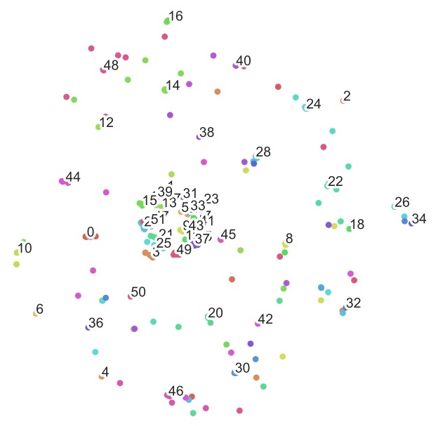
Figure 4: tSNE visualization of prototypes learned on dataset arts under mode PNML-multiple. Each point corresponds to one prototype, and prototypes belonging to the same positive or negative component of one label have the same color. Odd number locates at the mean of one label’s negative prototypes. Even number locates at the mean of one label’s positive prototypes. For example, number 0 indicates positive prototype mean of label 0, and number 1 indicates negative prototype mean of label 0.

Besides, in our PNML, label dependency is encoded into prototypes, especially positive prototypes. Intuitively, if label $j$ and label $k$ have high positive label dependency, they should have many common positive instances, and thus similar positive prototypes. Figure 5 shows the roughly estimated label dependency represented by correlation coefficients computed by label matrix columns. In Figure 5, label correlation coefficients of dataset arts is showed and for the clear view of highly correlated labels, correlation coefficients $coef<0.1$ and $coef>-0.1$ are set to 0. Compare Figure 4 with Figure 5, we can observe that prototypes present the label dependency. For example, in Figure 5, label 7 has high correlation coefficients with label 20 and label 24, and you can observe in Figure 4 that the positive prototypes of these three labels (located by number 14, 40 and 48) stay close. An negatively correlatted example is the label 15 and label 22. You can observe that they have correlation coefficient $-0.2$ and the positive prototypes of them (located by number 30 and 44) are far away from each other.

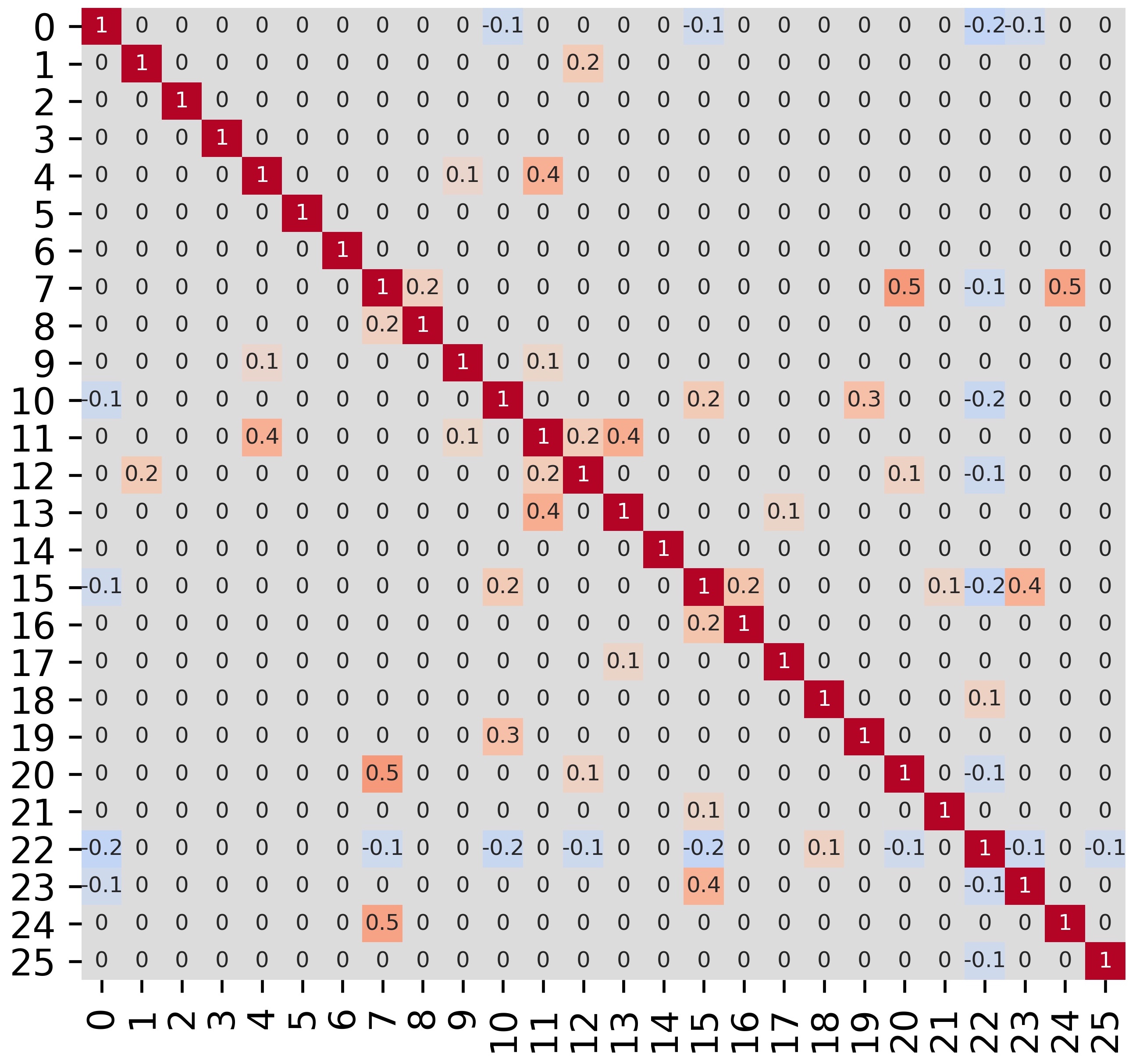
Figure 5: Correlation coefficients computed by label matrix of dataset arts. Correlation coefficients $coef<0.1$ and $coef>-0.1$ are set to zero

Parameter Sensitivity

In this part, we show the sensitivity of parameters. There are four/five hyperparameters in mode PNML-single/PNML-multiple, $M$ for embedding dimension, $\beta$ for slope of LeakyRelu, $\alpha$ for concentration parameter to determine the distance threshold (only used in mode PNML-multiple) and $\lambda_{\_}1$, $\lambda_{\_}2$ for loss tradeoff parameters. $\beta$ is setted as $0.2$ and $M$ is setted by Equation 14 in our paper. These two parameters are empirically setted and work well for all datasets we used. For $\lambda_{\_}1$, $\lambda_{\_}2$ and $\alpha$, Figure 6 shows their sensitivity test on dataset emotions with metric Micro-averaging $F_{\_}{1}$ under mode PNML-multiple. The sensitivity test results for $\lambda_{\_}1$ and $\lambda_{\_}2$ under mode PNML-single will not be shown here since the similar trends.

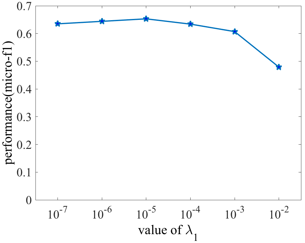
(a) $\lambda_{\_}1$

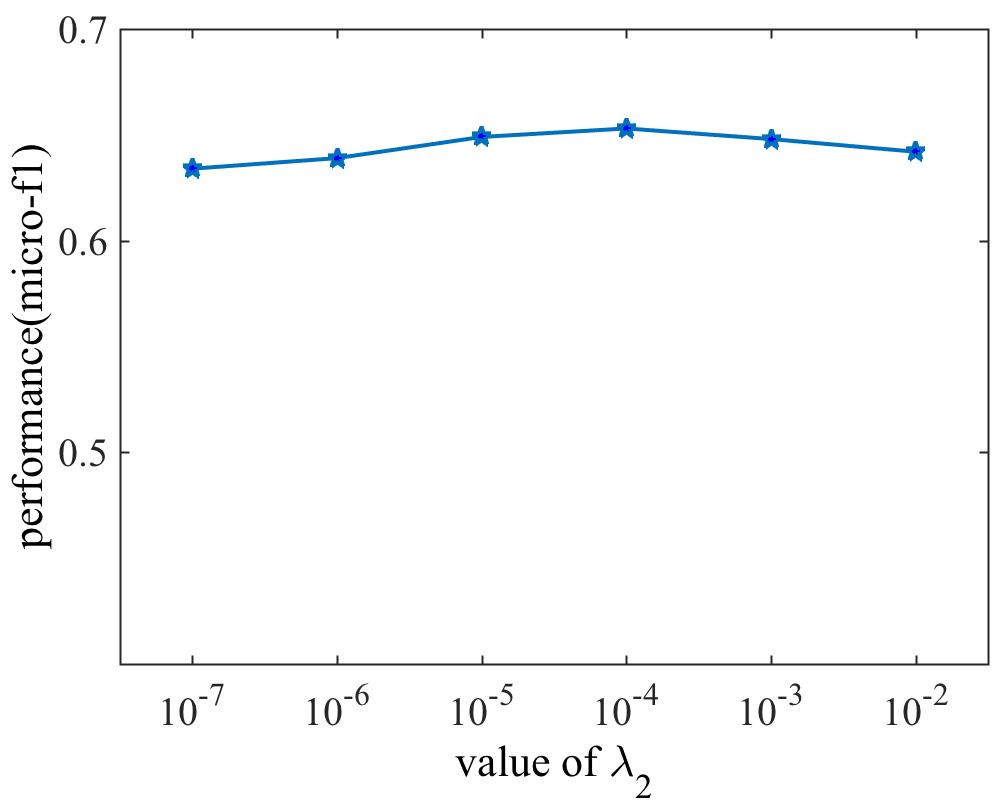
(b) $\lambda_{\_}2$

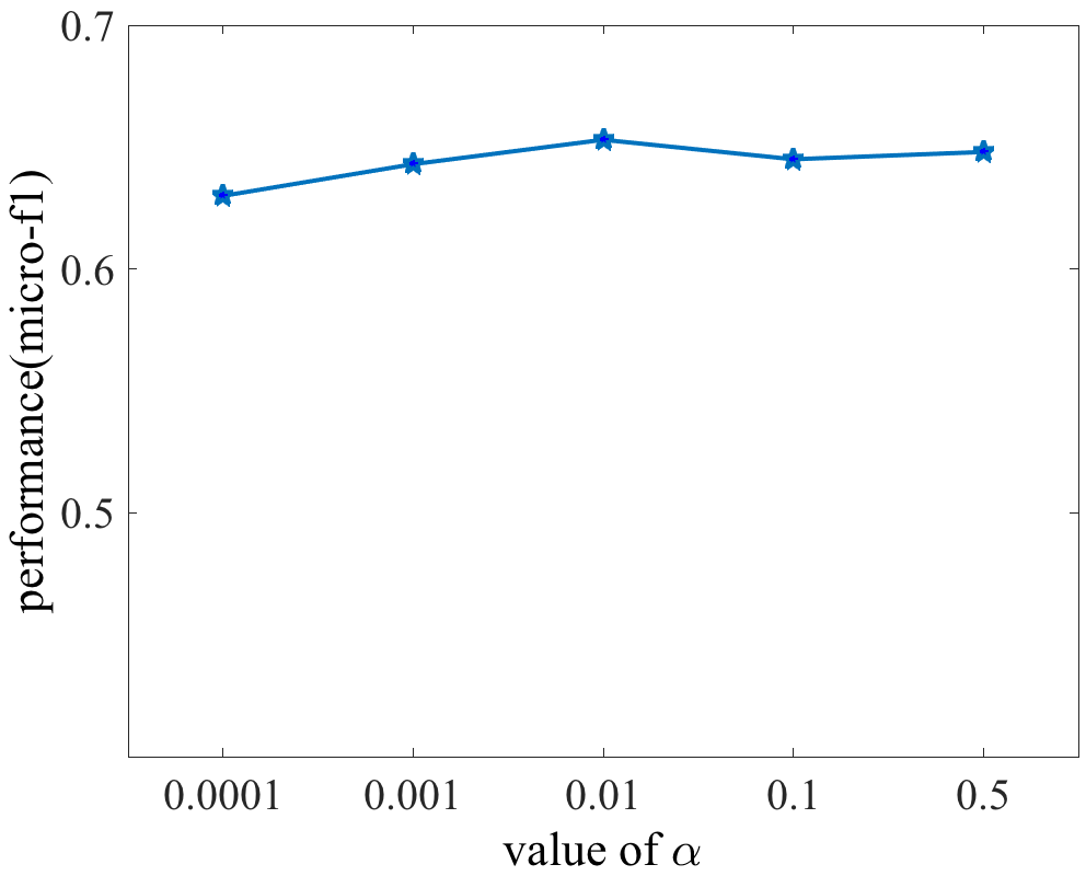
(c) $\alpha$

Figure 6: Parameter sensitivity on dataset emotions under mode PNML-multiple

References

- Allen et al. (2019) Allen, K.; Shelhamer, E.; Shin, H.; and Tenenbaum, J. 2019. Infinite Mixture Prototypes for Few-shot Learning. In Proceedings of the 36th International Conference on Machine Learning.
- Banerjee et al. (2005) Banerjee, A.; Merugu, S.; Dhillon, I. S.; and Ghosh, J. 2005. Clustering with bregman divergences. Journal of machine learning research 6: 1705–1749.
- Bhatia et al. (2015) Bhatia, K.; Jain, H.; Kar, P.; Varma, M.; and Jain, P. 2015. Sparse Local Embeddings for Extreme Multi-label Classification. In Proceedings of the 28th International Conference on Neural Information Processing Systems, 730–738. Montreal, Canada.
- Cai et al. (2013) Cai, X.; Nie, F.; Cai, W.; and Huang, H. 2013. New graph structured sparsity model for multi-label image annotations. In Proceedings of the 2013 IEEE International Conference on Computer Vision, 801–808. Sydney, NSW, Australia.
- Chen et al. (2016) Chen, W.; Yuanhai, S.; Chunna, L.; and Naiyang, D. 2016. MLTSVM: a novel twin support vector machine to multi-label learning. Pattern Recognition .
- Chen et al. (2019) Chen, Z.; Wei, X.; Wang, P.; and Guo, Y. 2019. Multi-Label Image Recognition with Graph Convolutional Networks. In Proceedings of 2019 IEEE Conference on Computer Vision and Pattern Recognition, 5177–5186. Long Beach, CA.
- Demsar (2006) Demsar, J. 2006. Statistical Comparisons of Classifiers over Multiple Data Sets. Journal of Machine Learning Research .
- Feng, An, and He (2019) Feng, L.; An, B.; and He, S. 2019. Collaboration based Multi-Label Learning. In Proceedings of the 33rd AAAI Conference on Artificial Intelligence, 3550–3557. Honolulu, Hawaii: AAAI Press.
- Guo (2017) Guo, Y. 2017. Convex co-embedding for matrix completion with predictive side information. In Proceedings of the Thirty-First AAAI Conference on Artificial Intelligence, 1955–1961. San Francisco, California, USA.
- Huang et al. (2018) Huang, J.; Li, G.; Huang, Q.; and Wu, X. 2018. Joint Feature Selection and Classification for Multilabel Learning. IEEE TRANSACTIONS ON CYBERNETICS 48: 876–889.
- Kingma and Ba (2015) Kingma, D.; and Ba, J. L. 2015. Adam: A Method for Stochastic Optimization. In Proceedings of the 3rd International Conference on Learning Representations. San Diego.
- Kulis and Jordan (2012) Kulis, B.; and Jordan, M. I. 2012. Revisiting k-means: New Algorithms via Bayesian Nonparametrics. In Proceedings of the 29th International Conference on Machine Learning.
- Li, Ouyang, and Zhou (2015) Li, X.; Ouyang, J.; and Zhou, X. 2015. Supervised topic models for multi-label classification. Neurocomputing 149: 811–819.
- Lin et al. (2014) Lin, Z.; Ding, G.; Hu, M.; and Wang, J. 2014. Multi-label Classification via Feature-aware Implicit Label Space Encoding. In Proceedings of the 31st International Conference on Machine Learning. Beijing, China.
- Liu and Tsang (2015) Liu, W.; and Tsang, I. W. 2015. Large Margin Metric Learning for Multi-label Prediction. In Proceedings of the 29th AAAI Conference on Artificial Intelligence, 2800–2806. Austin Texas, USA.
- Maas, Hannun, and Ng (2013) Maas, A. L.; Hannun, A. Y.; and Ng, A. Y. 2013. Rectifier Nonlinearities Improve Neural Network Acoustic Models. In Proceedings of the 30th International Conference on Machine Learning. Atlanta, Georgia, USA.
- Parameswaran and Weinberger (2010) Parameswaran, S.; and Weinberger, K. Q. 2010. Large margin multi-task metric learning. In Proceedings of the 23rd International Conference on Neural Information Processing Systems, 1867–1875. Vancouver, British Columbia, Canada.
- Prabhu et al. (2018) Prabhu, Y.; Kag, A.; Harsola, S.; Agrawal, R.; and Varma, M. 2018. Parabel: Partitioned label trees for extreme classification with application to dynamic search advertising. In Proceedings of the 27th International Conference on World Wide Web.
- R.Boutell et al. (2004) R.Boutell, M.; Luo, J.; Shen, X.; and M.Browna, C. 2004. Learning multi-label scene classification. Pattern Recognition 37: 1757–1771.
- Rubin et al. (2012) Rubin, T. N.; Chambers, A.; Smyth, P.; and Steyvers, M. 2012. Statistical topic models for multi-label document classification. Machine Learning 88: 157–208.
- Snell, Swersky, and Zemel (2017) Snell, J.; Swersky, K.; and Zemel, R. 2017. Prototypical Networks for Few-shot Learning. In Proceedings of the 30th International Conference on Neural Information Processing Systems. Long Beach, CA.
- Sorower (2010) Sorower, M. S. 2010. A Literature Survey on Algorithms for Multi-label Learning .
- Szymański and Kajdanowicz (2017) Szymański, P.; and Kajdanowicz, T. 2017. A scikit-based Python environment for performing multi-label classification. ArXiv e-prints .
- Tai and Lin (2012) Tai, F.; and Lin, H.-T. 2012. Multilabel classification with principal label space transformation. Neural Computation 24: 2508–2542.
- Tsoumakas and Vlahavas (2007) Tsoumakas, G.; and Vlahavas, I. 2007. Random k-labelsets: An ensemble method for multilabel classification. In Proceedings of the 18th European conference on Machine Learning, 406–417. Warsaw, Poland.
- Weinberger and Saul (2009) Weinberger, K. Q.; and Saul, L. K. 2009. Distance Metric Learning for Large Margin Nearest Neighbor Classification. Journal of Machine Learning Research 10: 207–244.
- Xu et al. (2014) Xu, L.; Wang, Z.; Shen, Z.; Wang, Y.; and Chen, E. 2014. Learning Low-Rank Label Correlations for Multi-label Classification with Missing Labels. In Proceedings of 2014 IEEE International Conference on Data Mining, 1067–1072. Shenzhen, China.
- Yang et al. (2016) Yang, H.; Zhou, J. T.; Zhang, Y.; Gao, B.-B.; Wu, J.; and Cai, J. 2016. Exploit Bounding Box Annotations for Multi-label Object Recognition. In Proceedings of 2016 IEEE Conference on Computer Vision and Pattern Recognition, 280–288. Las Vegas.
- Yu et al. (2012) Yu, G.; Domeniconi, C.; Rangwala, H.; Zhang, G.; and Yu, Z. 2012. Transductive multi-label ensemble classification for protein function prediction. In Proceedings of the 18th ACM SIGKDD international conference on Knowledge discovery and data mining, 1077–10856. Beijing, China.
- Yu et al. (2014) Yu, H.-F.; Jain, P.; Kar, P.; and Dhillon, I. S. 2014. Large-scale multi-label learning with missing labels. In Proceedings of the 31st International Conference on Machine Learning, 593–691. Beijing, China.
- Zhang (2011) Zhang, M. 2011. LIFT: Multi-Label Learning with Label-Specific Features. In Proceedings of the 22nd International Joint Conference on Artificial Intelligence, 1609–1614. Barcelona, Catalonia, Spain.
- Zhang and Zhou (2007) Zhang, M.; and Zhou, Z. 2007. Ml-knn: A Lazy Learning Approach to Multi-Label Learning. Pattern Recognition 40: 2038–2048.
- Zhang and Schneider (2012) Zhang, Y.; and Schneider, J. G. 2012. Maximum Margin Output Coding. In Proceedings of the 29th International Conference on Machine Learning. Edinburgh, Scotland, UK.