h KA-TP-21-2019
h IFIRSE-TH-2019-8
Gauge Dependences of Higher-Order Corrections to
NMSSM Higgs Boson Masses and
the Charged Higgs Decay $H^{\pm}\rightarrow W^{\pm}h_{i}$

Abstract

In this paper we compute the electroweak corrections to the charged Higgs boson decay into a $W$ boson and a neutral Higgs boson in the CP-conserving NMSSM. We calculate the process in a general $R_{\xi}$ gauge and investigate the dependence of the loop-corrected decay width on the gauge parameter $\xi$. The gauge dependence arises from the mixing of different loop orders. Phenomenology requires the inclusion of mass and mixing corrections to the external Higgs bosons in order to match the experimentally measured mass values. As a result, we move away from a strict one-loop calculation and consequently mix orders in perturbation theory. Moreover, determination of the loop-corrected masses in an iterative procedure also results in the mixing of different loop orders. Gauge dependence then arises from the mismatch with tree-level Goldstone boson couplings that are applied in the loop calculation, and from the gauge dependence of the loop-corrected masses themselves. We find that the gauge dependence is significant.

1 Introduction

The discovery of the Higgs boson by the LHC experiments ATLAS and CMS [1, 2] structurally completed the Standard Model (SM). Subsequent measurements revealed a very SM-like behavior of the Higgs boson. Due to open questions that cannot be answered within the SM, however, theories beyond the SM are considered, many of which contain extended Higgs sectors. So far, no direct signs of New Physics have been observed. This moves the Higgs sector itself into the focus of searches for indirect manifestations beyond the SM. Due to the very SM-like nature of the Higgs boson, sophisticated experimental techniques together with precise theoretical predictions are required for these investigations to be successful. In particular, higher-order (HO) corrections to the Higgs boson observables, their production cross sections, decay widths, and branching ratios have to be taken into account.

A clear manifestation of extended Higgs sectors would be the discovery of a charged Higgs boson that is not present in the SM. Charged Higgs bosons appear e.g. in the next-to-minimal supersymmetric extension of the SM (NMSSM) [3, 4, 5, 6, 7, 8, 9, 10, 11, 12, 13, 14] which is the model that we consider in this work. More specifically, we work in the framework of the scale-invariant CP-conserving NMSSM. The main decay channels of the charged Higgs boson are those into fermionic final states, but also decays into a Higgs and gauge boson final state, or into electroweakinos can become numerically important depending on the specific parameter values. In this paper, we compute the electroweak corrections to the decay of the charged Higgs boson into a $W$ boson and a light CP-even Higgs boson. We restrict ourselves to pure on-shell decays. The aim of this paper is not only to quantify the relative importance of the electroweak corrections, but in particular we also highlight problems with respect to gauge dependences that occur in the computation of the HO corrections. In a gauge theory gauge-breaking effects do not appear when the computation is restricted to a fixed order, here the one-loop level. This changes, however, when different loop orders are mixed, see e.g. also the discussions in [15, 16, 17, 18, 19, 20, 21, 22, 23, 24]. We encounter such a mixing when we include loop corrections to the mass of the involved external Higgs boson. Since the tree-level upper bound of the SM-like Higgs boson is below the observed $125.09$ GeV [25], loop corrections have to be included to shift its mass to the measured value. This introduces a mismatch between the loop-corrected mass of the external neutral Higgs boson and its corresponding tree-level mass, which is used in the propagators of the internal lines and in the tree-level Higgs-Goldstone boson couplings that occur in the computation of the one-loop amplitude. While the latter can be cured by an appropriate change of the Higgs-Goldstone boson coupling as we will outline below (see also [18, 19, 21, 22, 23] for a discussion), the former cannot be cured by introducing loop-corrected masses for the internal lines since it will break UV finiteness. Furthermore, we encounter additional gauge dependences due to the gauge dependence of the loop-corrected Higgs boson masses and their loop-corrected mixing matrix. The loop-corrected Higgs boson masses are defined through the complex poles of the propagator matrix which are evaluated by using an iterative method. While this method gives precise values of the complex poles, it mixes the contributions of different orders of perturbation theory and therefore introduces a dependence on the gauge parameter. The loop-corrected mixing matrix is used to resum the large corrections that stem from the mixing between different neutral Higgs bosons so that the loop corrections remain small and the higher-order prediction are reliable. In addition, the loop-corrected mixing matrix ensures the on-shell property of the external Higgs boson. This mixing matrix is, however, gauge dependent by definition. With the loop corrections to the light Higgs boson masses and the mixing matrix being substantial also the gauge dependence turns out to be significant and much more important than in the minimal supersymmetric extension of the SM (MSSM) as discussed in this work. The purpose of the present paper is to quantify this effect and to investigate different approximations with respect to their gauge dependences.

The outline of the paper is as follows. In Sec. 2 we introduce the Higgs sector of the NMSSM at tree level and at higher orders, and set our notation. In Sec. 3 we describe our computation of the electroweak one-loop corrections to the charged Higgs decay into a gauge plus Higgs boson final state. In particular we present the decay width at strict one-loop order. We follow up with a general discussion of gauge dependences encountered in the decay before presenting improved effective decay widths that include higher-order-corrected external Higgs states in different approximations. In the numerical results of Sec. 4 we analyze the gauge dependence of the loop-corrected masses themselves and subsequently the decay amplitudes and decay widths. We analyze the latter two with respect to their gauge dependences by including various approximations in the treatment of the loop-corrected external Higgs states. We also compare the results with the the size of the gauge dependences in the MSSM limit. We conclude with a small discussion of the relative size of the electroweak corrections as a function of the relevant NMSSM parameters. In Sec. 5 we summarize our results.

2 Higgs sector of the NMSSM

In this paper, we calculate within the NMSSM the one-loop corrections to the decays of the charged Higgs boson into a $W^{\pm}$ boson and a neutral CP-even Higgs boson. To that end, we briefly introduce the Higgs sector of the NMSSM and set up the notation required both for the calculation of the charged Higgs decays as well as for the discussion of the higher-order-corrected neutral Higgs boson masses. Since we apply the same approximations and renormalization conditions as in our previous works on higher-order corrections to the NMSSM Higgs boson masses and trilinear self-couplings [26, 27, 28, 29, 20, 30], we remain here as brief as possible and refer, where appropriate, to the corresponding literature for more information. We work in the framework of an NMSSM wherein a gauge-singlet chiral superfield $\hat{S}$ is added to the MSSM field content, and the superpotential couplings of this singlet are constrained by a $\mathbb{Z}_{3}$ symmetry. In terms of the two Higgs doublet superfields $\hat{H}_{u}$ and $\hat{H}_{d}$ and the singlet superfield $\hat{S}$ the NMSSM superpotential is written as

$$\mathcal{W}_{\text{NMSSM}}=\mathcal{W}_{\text{MSSM}}+\frac{1}{3}\kappa{\hat{S}}^{3}-\epsilon_{ij}\lambda\hat{S}\hat{H}_{d}^{i}\hat{H}_{u}^{j}\,,$$ (1)

with the totally antisymmetric tensor $\epsilon_{ij}$ ($i,j=1,2$) and $\epsilon_{12}=\epsilon^{12}=1$, where $i,j$ denote the indices of the fundamental $SU(2)_{L}$ representation. Working in the framework of the CP-conserving NMSSM, the dimensionless parameters $\lambda$ and $\kappa$ are taken to be real. The MSSM superpotential $\mathcal{W}_{\text{MSSM}}$ is expressed in terms of the quark and lepton superfields and their charge conjugates as denoted by the superscript $c$, i.e. $\hat{Q},\hat{U}^{c},\hat{D}^{c},\hat{L}$ and $\hat{E}^{c}$, as

$$\mathcal{W}_{\text{MSSM}}=\epsilon_{ij}[y_{e}\hat{H}^{i}_{d}\hat{L}^{j}\hat{E}^{c}+y_{d}\hat{H}_{d}^{i}\hat{Q}^{j}\hat{D}^{c}-y_{u}\hat{H}^{i}_{u}\hat{Q}^{j}\hat{U}^{c}]\,.$$ (2)

For better readability, the color and generation indices have been suppressed, and $\mu$ (i.e. the supersymmetric Higgs mass parameter of the MSSM) is set to 0 due to the applied $\mathbb{Z}_{3}$ symmetry. We neglect flavor mixing so that the Yukawa couplings $y_{u},y_{d}$ and $y_{e}$, which in general are $3\times 3$ matrices in flavor space, are diagonal.

The soft supersymmetry (SUSY) breaking NMSSM Lagrangian is given in terms of the scalar component fields $H_{u}$, $H_{d}$ and $S$ by

$${\cal L}_{\text{soft},\text{ NMSSM}}= -m_{H_{d}}^{2}H_{d}^{\dagger}H_{d}-m_{H_{u}}^{2}H_{u}^{\dagger}H_{u}-m_{\tilde{Q}}^{2}\tilde{Q}^{\dagger}\tilde{Q}-m_{\tilde{L}}^{2}\tilde{L}^{\dagger}\tilde{L}-m_{\tilde{u}_{R}}^{2}\tilde{u}_{R}^{*}\tilde{u}_{R}-m_{\tilde{d}_{R}}^{2}\tilde{d}_{R}^{*}\tilde{d}_{R}$$

$$-m_{\tilde{e}_{R}}^{2}\tilde{e}_{R}^{*}\tilde{e}_{R}-(\epsilon_{ij}[y_{e}A_{e}H_{d}^{i}\tilde{L}^{j}\tilde{e}_{R}^{*}+y_{d}A_{d}H_{d}^{i}\tilde{Q}^{j}\tilde{d}_{R}^{*}-y_{u}A_{u}H_{u}^{i}\tilde{Q}^{j}\tilde{u}_{R}^{*}]+\mathrm{h.c.})$$

$$-\frac{1}{2}(M_{1}\tilde{B}\tilde{B}+M_{2}\tilde{W}_{j}\tilde{W}_{j}+M_{3}\tilde{G}\tilde{G}+\mathrm{h.c.})$$ (3)

$$-m_{S}^{2}|S|^{2}+(\epsilon_{ij}\lambda A_{\lambda}SH_{d}^{i}H_{u}^{j}-\frac{1}{3}\kappa A_{\kappa}S^{3}+\mathrm{h.c.})\;,$$

where the summation over all three quark and lepton generations is implicit. Here, we denote by $\tilde{Q}$ and $\tilde{L}$ the complex scalar components of the corresponding left-handed quark and lepton superfields, so that e.g. for the first generation we have $\tilde{Q}=(\tilde{u}_{L},\tilde{d}_{L})^{T}$ and $\tilde{L}=(\tilde{\nu}_{L},\tilde{e}_{L})^{T}$. The $M_{k}$ ($k=1,2,3$) represent the gaugino mass parameters of the bino, wino and gluino fields $\tilde{B}$, $\tilde{W}_{j}$ ($j=1,2,3$) and $\tilde{G}$, the $m_{X}^{2}$ are the squared soft SUSY-breaking mass parameters of the scalar fields $X=S,H_{d},H_{u},\tilde{Q},\tilde{u}_{R},\tilde{d}_{R},\tilde{L},\tilde{e}_{R}$ and $A_{x}$ ($x=\lambda,\kappa,d,u,e$) are the soft SUSY-breaking trilinear couplings. In general, the soft SUSY-breaking trilinear couplings and the gaugino mass parameters can be complex, but in the limit of CP conservation all parameters are taken to be real.

2.1 The Higgs Sector at Tree Level

The Higgs potential at tree level reads

$$V_{H} = (|\lambda S|^{2}+m_{H_{d}}^{2})H_{d}^{\dagger}H_{d}+(|\lambda S|^{2}+m_{H_{u}}^{2})H_{u}^{\dagger}H_{u}+m_{S}^{2}|S|^{2}$$

$$+\frac{1}{8}(g_{2}^{2}+g_{1}^{2})(H_{d}^{\dagger}H_{d}-H_{u}^{\dagger}H_{u})^{2}+\frac{1}{2}g_{2}^{2}|H_{d}^{\dagger}H_{u}|^{2}$$

$$+|-\epsilon^{ij}\lambda H_{d,i}H_{u,j}+\kappa S^{2}|^{2}+\big{[}-\epsilon^{ij}\lambda A_{\lambda}SH_{d,i}H_{u,j}+\frac{1}{3}\kappa A_{\kappa}S^{3}+\mathrm{h.c.}\big{]}\;,$$

with $g_{1}$ and $g_{2}$ being the $U(1)_{Y}$ and $SU(2)_{L}$ gauge couplings, respectively. The two Higgs doublets and the singlet can be expanded around their vacuum expectation values (VEVs) $v_{u},v_{d}$ and $v_{s}$ as

$$H_{u}=\matrixquantity(h_{u}^{+}\\ \frac{1}{\sqrt{2}}(v_{u}+h_{u}+ia_{u})),\quad H_{d}=\matrixquantity(\frac{1}{\sqrt{2}}(v_{d}+h_{d}+ia_{d})\\ h_{d}^{-})\quad\mbox{and}\quad S=\frac{1}{\sqrt{2}}(v_{s}+h_{s}+ia_{s})\,.$$ (5)

The fields $h_{u},h_{d}$ and $h_{s}$ are the CP-even parts and $a_{u}$, $a_{d}$ and $a_{s}$ are the CP-odd parts of the neutral components of the fields $H_{u}$, $H_{d}$ and $S$, respectively. The electrically charged components are denoted by $h^{+}_{u}$ and $h^{-}_{d}$. The VEVs of the two Higgs doublets, $v_{u}$ and $v_{d}$, are related to the VEV $v\approx 246$ GeV of the SM as

$$v^{2}=v_{u}^{2}+v_{d}^{2}\,,$$ (6)

with the ratio between them being defined as

$$\tan\beta=\frac{v_{u}}{v_{d}}\,,$$ (7)

such that $v_{u}$ and $v_{d}$ can be expressed in terms of $v$ and $\tan\beta$. The potential $V_{H}$ is minimized by the VEVs, which implies that the first derivatives of the potential with respect to the Higgs fields must be zero. This leads to the definition of the tadpole parameters $t_{\phi}$,

$$t_{\phi}\equiv\left<\frac{\partial V_{H}}{\partial\phi}\right>\,,\quad\phi\in\quantity{h_{u},h_{d},h_{s},a_{u},a_{d},a_{s}}\,,$$ (8)

which have to vanish. Since we are working in CP-conserving NMSSM, the tadpole parameters that we have at tree level are given by

$$t_{h_{d}} =\frac{\lambda}{2}\left(-\sqrt{2}v_{s}v_{u}A_{\lambda}+\lambda v_{d}(v_{s}^{2}+v_{u}^{2})-\kappa v_{s}^{2}v_{u}\right)+\frac{1}{8}(g_{1}^{2}+g_{2}^{2})v_{d}(v_{d}^{2}-v_{u}^{2})+m_{H_{d}}^{2}v_{d}$$ (9)

$$t_{h_{u}} =\frac{\lambda}{2}\left(-\sqrt{2}v_{s}v_{d}A_{\lambda}+\lambda v_{u}(v_{s}^{2}+v_{d}^{2})-\kappa v_{s}^{2}v_{d}\right)+\frac{1}{8}(g_{1}^{2}+g_{2}^{2})v_{u}(v_{u}^{2}-v_{d}^{2})+m_{H_{u}}^{2}v_{u}$$ (10)

$$t_{h_{s}} =\frac{v_{s}}{2}\left(\sqrt{2}v_{s}\kappa A_{\kappa}+\lambda^{2}(v_{d}^{2}+v_{u}^{2})-2v_{d}v_{u}\kappa\lambda+2\kappa^{2}v_{s}^{2}\right)-\frac{1}{\sqrt{2}}v_{d}v_{u}\lambda A_{\lambda}+m_{S}^{2}v_{s}\leavevmode\nobreak\ .$$ (11)

In the CP-conserving NMSSM, there is no mixing between CP-even and CP-odd Higgs fields so that the bilinear parts of the Higgs potential read

$$V_{H}\supset\begin{pmatrix}h_{d}^{+}&h_{u}^{+}\end{pmatrix}\mathbb{M_{H^{\pm}}}\begin{pmatrix}h_{d}^{-}\\ h_{u}^{-}\end{pmatrix}+\frac{1}{2}\begin{pmatrix}h_{d}&h_{u}&h_{s}\end{pmatrix}\mathbb{M_{h}}\begin{pmatrix}h_{d}\\ h_{u}\\ h_{s}\end{pmatrix}+\frac{1}{2}\begin{pmatrix}a_{d}&a_{u}&a_{s}\end{pmatrix}\mathbb{M_{a}}\begin{pmatrix}a_{d}\\ a_{u}\\ a_{s}\end{pmatrix}\,,$$ (12)

with separate mass matrices $\mathbb{M_{H^{\pm}}},\mathbb{M_{h}}$ and $\mathbb{M_{a}}$ for the charged, CP-even and CP-odd Higgs fields, respectively. The explicit expressions of these tree-level mass matrices can be found in [26]. The charged, neutral CP-even and CP-odd mass eigenstates are obtained from the interaction states through rotations with the unitary matrices ${R^{H^{\pm}}}$, $R^{h}$ and $R^{a}$ as

$$\matrixquantity(G^{\pm}\\ H^{\pm})=R^{H^{\pm}}\matrixquantity(h_{d}^{\pm}\\ h_{u}^{\pm}),\quad\matrixquantity(h_{1}\\ h_{2}\\ h_{3})=R^{h}\matrixquantity(h_{d}\\ h_{u}\\ h_{s})\quad\text{and}\quad\matrixquantity(G^{0}\\ a_{1}\\ a_{2})=R^{a}\matrixquantity(a_{d}\\ a_{u}\\ a_{s})\,.$$ (13)

These rotation matrices diagonalize the mass matrices such that

$$\mathbb{M_{H^{\pm}}^{\text{diag}}}=R^{H^{\pm}}\mathbb{M_{H^{\pm}}}{R^{H^{\pm}}}^{\dagger},\,\,\,\,\mathbb{M_{h}^{\text{diag}}}=R^{h}\mathbb{M_{h}}{R^{h}}^{\dagger}\,\,\,\,\text{and}\,\,\,\,\mathbb{M_{a}^{\text{diag}}}=R^{a}\mathbb{M_{a}}{R^{a}}^{\dagger}.$$ (14)

The obtained mass eigenstates are ordered by ascending mass so that we have three CP-even Higgs states $h_{i}$ ($i=1,2,3$) with masses $m_{h_{1}}\leq m_{h_{2}}\leq m_{h_{3}}$, two CP-odd states $a_{j}$ ($j=1,2$) with masses $m_{a_{1}}\leq m_{a_{2}}$ and a charged Higgs pair $H^{\pm}$ with mass $m_{H^{\pm}}$ as the physical Higgs bosons. The fields $G^{0},G^{\pm}$ form the massless charged and neutral Goldstone modes. In general, the analytic forms of the mass eigenvalues are rather intricate, but analytic expressions for expansions in special parameter regions can be found in [31]. On the other hand, the squared mass of the charged Higgs boson is at tree level given by the simple expression

$$m_{H^{\pm}}^{2}=M_{W}^{2}+\frac{\lambda v_{s}}{\sin\newline \vspace*{-3.5mm}2\beta}\left(\sqrt{2}A_{\lambda}+\kappa v_{s}\right)-\frac{\lambda v^{2}}{2}\;.$$ (15)

Note that analogous to the MSSM there is an upper bound on the squared SM-like Higgs boson mass at tree level. In the NMSSM, it is given by

$$M_{Z}^{2}\cos^{2}2\beta+\frac{\lambda^{2}v^{2}}{2}\sin^{2}2\beta\;.$$ (16)

In order to comply with the measured value of $m_{H}=125.09$ GeV [25], loop corrections therefore have to be included in the computation of the Higgs boson mass.

The Higgs potential in Eq. 2.1 is parametrized by the parameter set

$$m_{H_{d}}^{2},m_{H_{u}}^{2},m_{S}^{2},g_{1},g_{2},v_{d},v_{u},v_{s},\lambda,\kappa,A_{\lambda},A_{\kappa}\;.$$ (17)

For a physical interpretation, it is convenient to substitute some of these parameters with more intuitive ones, such as e.g. the masses of gauge bosons which are measurable quantities, or the tadpole parameters. We can use Eqs. (6) and (7) to eliminate $v_{u}$ and $v_{d}$ in favour of $v$ and $\tan\beta$, and Eqs. (9)-(11) to replace the soft SUSY-breaking parameters $m_{H_{d}}^{2},m_{H_{u}}^{2}$ and $m_{S}^{2}$ in $V_{H}$ with $t_{h_{d}}$, $t_{h_{u}}$ and $t_{h_{s}}$. Furthermore, $A_{\lambda}$ can be replaced by $m_{H^{\pm}}^{2}$ using Eq. (15). Finally, $g_{1},g_{2}$ and $v$ are substituted by the squared masses $M_{W}^{2}$ and $M_{Z}^{2}$ of the $W^{\pm}$ and $Z$ bosons and the electric charge $e$ via

$$M_{W}^{2}=\frac{v^{2}g_{2}^{2}}{4},\,\,\,\,M_{Z}^{2}=\frac{v^{2}(g_{1}^{2}+g_{2}^{2})}{4},\,\,\,\,\text{and}\,\,\,\,e=\frac{g_{1}g_{2}}{\sqrt{g_{1}^{2}+g_{2}^{2}}}\,.$$ (18)

In summary, our set of free parameters in the Higgs sector is given by

$$t_{h_{d}},t_{h_{u}},t_{h_{s}},m_{H^{\pm}}^{2},M_{W}^{2},M_{Z}^{2},e,\tan\beta,v_{s},\lambda,\kappa,A_{\kappa}\leavevmode\nobreak\ .$$ (19)

Finally, the MSSM limit of the NMSSM Higgs sector can be obtained by setting

$$\lambda\rightarrow 0,\,\kappa\rightarrow 0,\,\,\,\,\kappa/\lambda\equiv\text{constant},$$ (20)

and keeping all other parameters, including

$$\mu_{\text{eff}}\equiv\frac{\lambda v_{s}}{\sqrt{2}}$$ (21)

and $A_{\kappa}$, fixed. In this limit the mixing between singlet and doublet Higgs fields vanishes.

2.2 The Loop-Corrected Higgs Sector

For the determination of the loop-corrected Higgs boson masses, the UV-divergent self-energies have to be calculated. The divergent integrals are regularized by the SUSY-conserving dimensional reduction scheme [32, 33]. Evaluating the self-energies in $D=4-2\epsilon$ dimensions, the divergences can be parametrized by the regulator $\epsilon$, leading to poles $1/\epsilon$ in the limit of $\epsilon\rightarrow 0$, i.e. in physical $D=4$ space-time dimensions. Also in the one-loop corrections to the process $H^{\pm}\to W^{\pm}h_{i}$ we encounter UV divergences. The UV divergences are cancelled by the renormalization of the Higgs fields and the parameters relevant for the calculation. In order to do so, the bare parameters $p_{0}$ of the Lagrangian are replaced by the renormalized ones, $p$, and their corresponding counterterms, $\delta p$,

$$p_{0}=p+\delta p\leavevmode\nobreak\ .$$ (22)

Analogously, the bare fields $\phi_{0}$ in the Lagrangian are expressed via the renormalized fields $\phi$ and the wave-function renormalization constants (WFRCs) $Z_{\phi}$ as

$$\phi_{0}=\sqrt{Z_{\phi}}\phi=\left(1+\frac{\delta\newline \vspace*{-3.5mm}Z_{\phi}}{2}\right)\phi\,.$$ (23)

In accordance with our previous works on higher-order corrections to the NMSSM Higgs boson masses [26, 27, 28, 29], we apply a mixed on-shell (OS) and $\overline{\text{DR}}$ renormalization scheme to fix the parameter and WFRCs. The free parameters of Eq. (19) are defined to be either OS or $\overline{\text{DR}}$ parameters as follows

$$\underbrace{t_{h_{d}},t_{h_{u}},t_{h_{s}},m_{H^{\pm}}^{2},m_{W}^{2},m_{Z}^{2},e}_{\text{OS}},\underbrace{\tan\beta,v_{s},\lambda,\kappa,A_{\kappa}}_{\overline{\text{DR}}}\;.$$ (24)

The renormalization scheme for the parameters is chosen such that the quantities which can be related to physical observables are defined on-shell, whereas the rest of the parameters are defined as $\overline{\text{DR}}$ parameters. In addition, we introduce the WFRCs for the doublet and singlet fields before rotation into the mass eigenstates as

$$H_{d} \rightarrow\sqrt{Z_{H_{d}}}H_{d}=\left(1+\frac{\delta Z_{H_{d}}}{2}\right)H_{d}$$ (25)

$$H_{u} \rightarrow\sqrt{Z_{H_{u}}}H_{u}=\left(1+\frac{\delta Z_{H_{u}}}{2}\right)H_{u}$$ (26)

$$S \rightarrow\sqrt{Z_{S}}S=\left(1+\frac{\delta Z_{S}}{2}\right)S.$$ (27)

We apply $\overline{\text{DR}}$ conditions for the WFRCs of the Higgs fields. We introduce a WFRC for the $W$ boson field, needed in the computation of the loop corrections to the charged Higgs boson decay, as

$$W^{\pm}\to\sqrt{Z_{W}}W^{\pm}=\left(1+\frac{\delta Z_{W}}{2}\right)W^{\pm}\,.$$ (28)

The WFRC $\delta Z_{W}$ is defined through the OS condition

$$\delta Z_{W}=-\left.\frac{\partial\Sigma^{T}_{WW}}{\partial p^{2}}\right|_{p^{2}=M_{W}^{2}}\;,$$ (29)

where $\Sigma^{T}_{WW}$ denotes the transverse part of the $W$ boson self-energy.

The Higgs boson masses and hence the mixing matrices receive large radiative corrections. Therefore it is necessary to include these corrections at the highest order possible to improve the theoretical predictions. Recently, we completed the two-loop order ${\cal O}(\alpha_{t}^{2})$ corrections to the neutral Higgs boson masses in the CP-violating NMSSM [29], thus improving our previous results, which were available to two-loop order ${\cal O}(\alpha_{t}\alpha_{s})$ [28]. The Higgs boson masses corrected up to two-loop order ${\cal O}(\alpha_{t}\alpha_{s}+\alpha_{t}^{2})$ require also the renormalization of the top/stop sector at one-loop order. The computation of the two-loop corrections together with the renormalization of the parameters in the above defined mixed OS-$\overline{\mbox{DR}}$ scheme has been described in great detail in  [28, 29], hence we do not repeat it here and instead refer to these references for details. The CP-conserving limit of these results given in the CP-violating NMSSM is straightforward, further information can also be found in [26] where the one-loop calculation is presented for the real NMSSM. We review here, however, important points and highlight differences for the purpose of discussing the parameter dependence. In the following, we focus on the CP-even Higgs bosons. Their loop-corrected masses are defined as the real parts of the poles of the propagator matrix. These complex poles are the zeros of the determinant of the renormalized two-point correlation function $\hat{\Gamma}(p^{2})$, where $p^{2}$ denotes the external squared four-momentum. The renormalized two-point correlation function is expressed as

$$\hat{\Gamma}(p^{2}) = i\left(p^{2}\text{1}-\hat{M}^{2}_{S}(p^{2},\xi)\right)\;,$$ (30)

with

$$\hat{M}^{2}(p^{2},\xi) = \matrixquantity(m_{h_{1}}^{2}-\hat{\Sigma}_{h_{1}h_{1}}(p^{2},\xi)&-\hat{\Sigma}_{h_{1}h_{2}}(p^{2},\xi)&-\hat{\Sigma}_{h_{1}h_{3}}(p^{2},\xi)\\ -\hat{\Sigma}_{h_{2}h_{1}}(p^{2},\xi)&m_{h_{2}}^{2}-\hat{\Sigma}_{h_{2}h_{2}}(p^{2},\xi)&-\hat{\Sigma}_{h_{2}h_{3}}(p^{2},\xi)\\ -\hat{\Sigma}_{h_{3}h_{1}}(p^{2},\xi)&-\hat{\Sigma}_{h_{3}h_{2}}(p^{2},\xi)&m_{h_{3}}^{2}-\hat{\Sigma}_{h_{3}h_{3}}(p^{2},\xi))\;,$$ (31)

where the renormalized self-energy $\hat{\Sigma}_{h_{i}h_{j}}(p^{2},\xi)$ of the transition $h_{i}\to h_{j}$ ($i,j=1,2,3$) is given by

$$\hat{\Sigma}_{h_{i}h_{j}}(p^{2},\xi)=\hat{\Sigma}^{1l}_{h_{i}h_{j}}(p^{2},\xi)+\hat{\Sigma}^{\alpha_{t}\alpha_{s}}_{h_{i}h_{j}}(0)+\hat{\Sigma}^{\alpha_{t}^{2}}_{h_{i}h_{j}}(0)\;.$$ (32)

Here, $\hat{\Sigma}^{1l}(p^{2},\xi)$ denotes the full one-loop self-energy with full momentum-dependent contributions computed in general $R_{\xi}$ gauge, where $\xi$ stands for the gauge parameters $\xi_{W},\xi_{Z}$. The last two terms are the two-loop corrections of order ${\cal O}(\alpha_{t}\alpha_{s})$ [28] and ${\cal O}(\alpha_{t}^{2})$ [29], respectively, which are evaluated in the approximation of vanishing external momentum. These contributions do not introduce additional gauge-dependent terms in the renormalized self-energies as they are evaluated in the gaugeless limit. We want to point out that the full one-loop renormalized self-energies $\hat{\Sigma}^{1l}(p^{2},\xi)$ in general $R_{\xi}$ gauge are newly computed by us and implemented in NMSSMCALC. We computed them both in the standard tadpole scheme and in the Fleischer-Jegerlehner scheme and the results are identical. We apply the iterative procedure described and applied in [26] to extract the zeros of the determinant. In the first iterative step for the calculation of the $n^{\text{th}}$ CP-even Higgs boson mass, the squared external momentum in the renormalized self-energies is chosen to be at its squared tree-level mass value, i.e. $p^{2}=m_{h_{n}}^{2}$. The mass matrix $\hat{M}^{2}(p^{2},\xi)$ is then diagonalized, yielding the $n^{\text{th}}$ eigenvalue as a first approximation to the squared mass of the $n^{\text{th}}$ CP-even Higgs boson. In the next step of the iteration, this value is taken as the new OS value for $p^{2}$, and the mass matrix is again diagonalized. This procedure is repeated until the $n^{\text{th}}$ eigenvalue changes by less than $10^{-9}$ GeV² between two consecutive steps of the iteration. The resulting complex pole is denoted by $\tilde{M}_{H_{n}}^{2}$ and the loop-corrected Higgs mass by $M_{H_{n}}=\sqrt{{\rm Re}(\tilde{M}_{H_{n}}^{2})}$. The loop-corrected CP-even Higgs masses are sorted in ascending order $M_{H_{1}}<M_{H_{2}}<M_{H_{3}}$. Note that we denote the loop-corrected masses and Higgs mass eigenstates by capital letters $M$ and $H_{i}$, respectively, whereas the corresponding tree-level values and eigenstates are denoted by lowercase letters, i.e. $m$ and $h_{i}$. The iterative procedure automatically mixes different orders of perturbation theory and therefore introduces intricate gauge dependences. This will be investigated in more detail in the numerical section.

Besides the computation of the loop-corrected masses, the code NMSSMCALC allows us to compute the loop-corrected mixing matrices in several approximations which are discussed also in [57]. First, we introduce the matrix $R^{0}$ for the rotation of the mass matrix in the approximation of vanishing external momentum,

$$\text{diag}(M_{0,H_{1}}^{2},M_{0,H_{2}}^{2},M_{0,H_{3}}^{2})=R^{0}\hat{M}^{2}(0,\xi)(R^{0})^{T}\;.$$ (33)

The corresponding loop-corrected mass eigenvalues are denoted by an index 0, hence $M_{0,H_{i}}^{2}$ ($i=1,2,3$). In this approximation the mixing matrix $R^{0}$ is unitary, but does not capture the proper OS properties of the external loop-corrected states as momentum-dependent effects are neglected.

A different approach leads to the rotation matrix $R^{\text{mtree}}$. Here we diagonalize the mass matrix with the elements evaluated at fixed momentum squared which is given by the arithmetic average of the squared masses,

$$p_{\text{mtree}}^{2}=\frac{m_{h_{i}}^{2}+m_{h_{j}}^{2}}{2}\;.$$ (34)

We hence have

$$\left(\hat{M}^{2}(p_{\text{mtree}}^{2},\xi)\right)_{ij}=m_{h_{i}}^{2}\delta_{ij}-\hat{\Sigma}_{h_{i}h_{j}}\left(\frac{m_{h_{i}}^{2}+m_{h_{j}}^{2}}{2},\xi\right)\;,$$ (35)

and the corresponding mass values denoted by $M_{\text{mtree},H_{i}}^{2}$ are obtained through rotation with the matrix $R^{\text{mtree}}$ as

$$\text{diag}(M_{\text{mtree},H_{1}}^{2},M_{\text{mtree},H_{2}}^{2},M_{\text{mtree},H_{3}}^{2})=R^{\text{mtree}}\hat{M}^{2}(p_{\text{mtree}}^{2},\xi)(R^{\text{mtree}})^{T}\;.$$ (36)

By this approach we approximately take into account the momentum dependence of the self-energies (see [22] for a discussion).

The correct OS properties of the loop-corrected mass eigenstates are obtained by following the procedure described in [15], i.e. by multiplying the tree-level matrix $R^{h}$ with the finite wave-function normalization factors given by the $\mathbf{Z}$ matrix [15] for external OS Higgs bosons at higher orders,

$$\mathbf{Z}=\begin{pmatrix}\sqrt{\hat{Z}_{H_{1}}}&\sqrt{\hat{Z}_{H_{1}}}\hat{Z}_{H_{1}H_{2}}&\sqrt{\hat{Z}_{H_{1}}}\hat{Z}_{H_{1}H_{3}}\\ \sqrt{\hat{Z}_{H_{2}}}\hat{Z}_{H_{2}H_{1}}&\sqrt{\hat{Z}_{H_{2}}}&\sqrt{\hat{Z}_{H_{2}}}\hat{Z}_{H_{2}H_{3}}\\ \sqrt{\hat{Z}_{H_{3}}}\hat{Z}_{H_{3}H_{1}}&\sqrt{\hat{Z}_{H_{3}}}\hat{Z}_{H_{3}H_{2}}&\sqrt{\hat{Z}_{H_{3}}}\end{pmatrix}\;,$$ (37)

where

$$\hat{Z}_{i}=\frac{1}{\left(\frac{i}{\Delta_{ii}(p^{2})}\right)^{\prime}(\tilde{M}_{i}^{2})}\qquad\mbox{and}\qquad\hat{Z}_{ij}=\left.\frac{\Delta_{ij}(p^{2})}{\Delta_{ii}(p^{2})}\right|_{p^{2}=\tilde{M}_{i}^{2}}\;,$$ (38)

with the indices $i,j=H_{1},H_{2},H_{3}$. The prime denotes the derivative with respect to $p^{2}$. The quantity

$$\Delta=-\left[\hat{\Gamma}(p^{2})\right]^{-1}$$ (39)

is evaluated at the complex poles $\tilde{M}_{i}^{2}$. In contrast to the rotation matrices $R^{0}$ and $R^{\text{mtree}}$, which are unitary matrices, the $\mathbf{Z}$ matrix is not as it contains resummed higher-order contributions. If we want to compute the decay width at exact one-loop level, we therefore have to expand the $\mathbf{Z}$ matrix and take only the one-loop terms

where $(\hat{\Sigma}^{1l}(p^{2}))^{\prime}=\partial_{p^{2}}\hat{\Sigma}^{1l}(p^{2})$. Note that the $\hat{\Sigma}^{1l}$ are evaluated at the tree-level mass values $m_{h_{i}}^{2}$, since using loop-corrected masses would introduce higher-order effects.

3 Electroweak One-Loop Corrections to $H^{\pm}\to W^{\pm}h_{i}$

3.1 Decay Width at Leading Order

The decay of the charged Higgs boson $H^{\pm}$ into a $W^{\pm}$ boson and a CP-even neutral Higgs boson $h_{i}$ ($i=1,2,3$) depends on the coupling

$$g_{W^{-}h_{i}H^{+}}=g_{2}\quantity(R^{h}_{i1}\cos{\beta}-R^{h}_{i2}\sin\beta)\;,$$ (40)

The leading-order (LO) decay width can be written as

$$\Gamma_{H^{\pm}\rightarrow W^{\pm}h_{i}}=\frac{\lambda^{3/2}\left(m_{H^{\pm}}^{2},M_{W}^{2},m_{h_{i}}^{2}\right)}{64\pi m_{H^{\pm}}^{3}M_{W}^{2}}\left|\mathcal{M}^{\text{tree}}_{H^{\pm}\rightarrow W^{\pm}h_{i}}\right|^{2}\,.$$ (41)

with $\lambda(x,y,z)=x^{2}+y^{2}+z^{2}-2xy-2xz-2yz$ denoting the usual Källén function and $\mathcal{M}^{\text{tree}}_{H^{\pm}\rightarrow W^{\pm}h_{i}}$ the reduced matrix element, which for the tree-level decay is given by

$$\mathcal{M}^{\text{tree}}_{H^{\pm}\rightarrow W^{\pm}h_{i}}=ig_{W^{-}h_{i}H^{+}}\;.$$ (42)

We remind the reader that by $m_{h_{i}}$ we denote the tree-level mass of the final state Higgs boson.

3.2 Decay Width at Strict One-Loop Order

The next-to-leading order (NLO) decay width $\Gamma^{\text{NLO}}$ is given by the sum of the LO width $\Gamma^{\text{LO}}$, the virtual corrections $\Gamma^{\text{virt}}$ and the real corrections $\Gamma^{\text{real}}$ as

$$\Gamma^{\text{NLO}}=\Gamma^{\text{LO}}+\Gamma^{\text{virt}}+\Gamma^{\text{real}}\;.$$ (43)

The virtual corrections contain the counterterm contributions that cancel the UV divergences. The IR divergences in the real corrections cancel those in the virtual corrections. $\Gamma^{\text{virt}}$ is given by

$$\Gamma^{\text{virt}}=\frac{\lambda^{3/2}\left(m_{H^{\pm}}^{2},M_{W}^{2},m_{h_{i}}^{2}\right)}{64\pi m_{H^{\pm}}^{3}M_{W}^{2}}2\,\text{Re}\quantity(\mathcal{M}^{\text{tree}*}_{H^{\pm}\rightarrow W^{\pm}h_{i}}\mathcal{M}^{\text{virt}})\;.$$ (44)

Note that in Eq. (44) we set $p_{h_{i}}^{2}=m_{h_{i}}^{2}$, i.e. we set the external Higgs boson on its tree-level mass shell. We do the same in the LO decay width and the real corrections. In this way, we ensure that the NLO decay width $\Gamma^{\text{NLO}}$ remains at strict one-loop order by avoiding admixtures of higher orders through loop corrections to the mass. $\mathcal{M}^{\text{virt}}$ consists of the one-particle-irreducible (1PI) diagrams depicted in Fig. 1. They show the external leg corrections $\mathcal{M}^{\text{ext},h}$ and $\mathcal{M}^{\text{ext},H^{\pm}}$ to the neutral Higgs boson and to the charged Higgs boson, respectively, and the genuine vertex corrections $\mathcal{M}^{\text{vert}}$. They already include the counterterms and are hence finite. The corrections to the $W$ boson leg vanish due to the OS renormalization of the $W$ boson. We hence have

$$\mathcal{M}^{\text{virt}}=\mathcal{M}^{\text{vert}}+\mathcal{M}^{\text{ext},H^{\pm}}+\mathcal{M}^{\text{ext},h}\;.$$ (45)

\begin{overpic}[width=91.04742pt]{exth.pdf} \put(7.0,47.0){$H^{\pm}$} \put(80.0,80.0){$h_{i}$} \put(87.0,22.0){$W^{\pm}$} \put(45.0,55.0){$h_{j}$} \put(35.0,1.0){$\mathcal{M}^{\text{ext},h}$} \end{overpic}

\begin{overpic}[width=91.04742pt]{extHp.pdf} \put(3.0,47.0){$H^{\pm}$} \put(80.0,80.0){$h_{i}$} \put(87.0,22.0){$W^{\pm}$} \put(40.0,47.0){$\Phi$} \put(33.0,1.0){$\mathcal{M}^{\text{ext},H^{\pm}}$} \end{overpic}

\begin{overpic}[width=91.04742pt]{vertex.pdf} \put(7.0,47.0){$H^{\pm}$} \put(80.0,80.0){$h_{i}$} \put(87.0,22.0){$W^{\pm}$} \put(35.0,1.0){$\mathcal{M}^{\text{vert}}$} \end{overpic}

Figure 1: Generic diagrams contributing to $\mathcal{M}^{\text{virt}}$: corrections to the external legs of $h_{i}$ and $H^{\pm}$, $\mathcal{M}^{\text{ext},h}$ and $\mathcal{M}^{\text{ext},H^{\pm}}$, and genuine vertex corrections $\mathcal{M}^{\text{vert}}$. $\Phi$ stands for the fields $\Phi\in\{H^{\pm},G^{\pm},W^{\pm}\}$.

The amplitudes for the external leg contributions to the neutral and charged Higgs bosons, $\mathcal{M}^{\text{ext},h}$ and $\mathcal{M}^{\text{ext},H^{\pm}}$, respectively, can be factorized into the tree-level amplitude and the propagator corrections to the external legs. For $\mathcal{M}^{\text{ext},h}$ we obtain

$$\mathcal{M}^{\text{ext},h} =\sum_{j=1}^{3}\delta\mathbf{Z}^{\text{1l}}_{ij}\mathcal{M}^{\text{tree}}_{H^{\pm}\rightarrow W^{\pm}h_{j}}\;.$$ (46)

Note that here we apply $\delta\mathbf{Z}^{\text{1l}}_{ij}$ at strict one-loop order, defined as

$$\delta\mathbf{Z}^{\text{1l}}_{ij}=\mathbf{Z}^{\text{1l}}_{ij}-\delta_{ij}\;,$$ (47)

with the $\mathbf{Z}$ matrix at strict one-loop order, $\mathbf{Z}^{\text{1l}}$, given in Eq. (2.2). The charged Higgs WFRC is determined in the $\overline{\mbox{DR}}$ scheme so that there are finite contributions to the LSZ factor $\sqrt{\hat{Z}_{H^{\pm}}}$ at one-loop order,

$$\sqrt{\hat{Z}_{H^{\pm}}} \approx 1-\frac{\delta\hat{Z}_{H^{\pm}}}{2}=1-\frac{\text{Re}\Sigma_{H^{+}H^{-}}^{\prime}(m_{H^{\pm}}^{2})}{2}-\frac{\cos^{2}\beta\,\delta Z_{H_{d}}+\sin^{2}\beta\,\delta Z_{H_{u}}}{2}\,,$$ (48)

where the prime denotes the derivative with respect to the squared four-momentum.

The mixing between $H^{\pm}$ and $G^{\pm}$ can be related to the mixing between $H^{\pm}$ and $W^{\pm}$ by using the Slavnov-Taylor identity for the renormalized self-energies,

$$\hat{\Sigma}_{H^{+}G^{-}}(m_{H^{\pm}}^{2})=\frac{m_{H^{\pm}}^{2}}{M_{W}}\hat{\Sigma}_{H^{+}W^{-}}(m_{H^{\pm}}^{2})\;,$$ (49)

where $\hat{\Sigma}_{H^{+}W^{-}}(m_{H^{\pm}}^{2})$ denotes the renormalized truncated self-energy of the transition $H^{+}\,\to\,W^{+}$. The correction to the $H^{\pm}$ propagator thereby results in

$$\mathcal{M}^{\text{ext},H^{\pm}}= \frac{\delta\hat{Z}_{H^{\pm}}}{2}\mathcal{M}^{\text{tree}}_{H^{\pm}\rightarrow W^{\pm}h_{i}}+\frac{1}{M_{W}^{2}}\hat{\Sigma}_{H^{+}W^{-}}(m_{H^{\pm}}^{2})\,g_{h_{i}WW}\,,$$ (50)

where the coupling is given by

$$g_{h_{i}WW}=\frac{g_{2}^{2}}{2}v(c_{\beta}R_{i1}+s_{\beta}R_{i2})\;.$$ (51)

The genuine vertex corrections $\mathcal{M}^{\text{vert}}$ are given by the diagrams depicted in Fig. 2 plus the corresponding counterterm contributions that are not shown here. The vertex corrections comprise the 1PI diagrams given by the triangle diagrams with scalars, fermions and gauge bosons in the loops, and the diagrams involving four-particle vertices.

Figure 2: One-loop diagrams contributing to the pure vertex corrections at NLO. Here $u_{j},d_{j}$ denote up- and down-type quarks and $\nu_{j},e_{j}$ neutrinos and charged leptons for all three generations ($j=1,2,3$), $\tilde{u}_{l},\tilde{d}_{l}$ denote up- and down-type squarks and $\tilde{e}_{l},\tilde{\nu}_{l}$ denote charged sleptons and sneutrinos ($l=1,...,6$), $a_{k}$ ($k=1,2$) denote the pseudoscalar and $h_{i,m,n}$ ($i,m,n=1,2,3$) the scalar Higgs bosons, and $\tilde{\chi}_{a,b}^{0}$ ($a,b=1,...,5$) and $\tilde{\chi}_{r,s}^{\pm}$ ($r,s=1,2$) represent the neutralinos and charginos, respectively.

The counterterm amplitude is given by

$${\cal M}^{\text{CT}} = i\frac{\delta g_{2}}{2}\quantity(R^{h}_{i1}\cos{\beta}-R^{h}_{i2}\sin\beta)+i\frac{g_{2}}{2}\quantity(R^{h}_{i1}\cos{\beta}\delta Z_{H_{d}}-R^{h}_{i2}{\sin\beta\hskip 2.0pt}{\delta Z_{H_{u}}})$$ (52)

$$+ i\frac{g_{2}}{2}\quantity(R^{h}_{i1}\cos{\beta}-R^{h}_{i2}\sin\beta)\frac{\delta Z_{W}}{2}\;,$$

in terms of the WFRCs $\delta Z_{H_{d}}$, $\delta Z_{H_{u}}$ and $\delta Z_{W}$ and the counterterm $\delta g_{2}$ for the $SU(2)_{L}$ gauge coupling constant $g_{2}$, which in terms of the counterterms of our input parameters, cf. Eq. (24), reads

$$\delta g_{2}=\delta\left(\frac{e}{\sin{\theta_{W}}}\right)=\frac{g_{2}}{e}\delta e-g_{2}\frac{\cos^{2}\theta_{W}}{2\sin^{2}\theta_{W}}\quantity(\frac{\delta M_{Z}^{2}}{M_{Z}^{2}}-\frac{\delta M_{W}^{2}}{M_{W}^{2}})\;.$$ (53)

The vertex diagrams also contain IR divergences. These arise from the exchange of a soft virtual photon between the external legs (cf. diagrams 21 and 28 of Fig. 2). Also $\delta M_{W}^{2}$, $\delta Z_{W}$ and $\hat{Z}_{H^{+}H^{-}}$ are IR-divergent. These soft singularities in the virtual corrections are canceled by the IR-divergent contributions from real photon radiation [58, 59] in the process $H^{\pm}\rightarrow W^{\pm}h_{i}$$\gamma$. The process is independently gauge-invariant and most easily calculated in unitary gauge. The diagrams that contribute in unitary gauge to the process are shown in Fig. 3. They consist of the proper bremsstrahlung contributions, where a photon is radiated from the charged initial and final state particles, and the diagram involving a four-particle vertex with a photon.

Figure 3: Feynman diagrams contributing to $H^{\pm}\rightarrow W^{\pm}h_{i}$$\gamma$ in the unitary gauge.

The decay width for the real emission is given by

$$\Gamma^{\text{real}}\equiv\Gamma_{H^{\pm}\rightarrow W^{\pm}h_{i}\gamma} = \frac{\alpha g^{2}_{W^{-}h_{i}H^{+}}}{4\pi^{2}m_{H^{\pm}}}\bigg{[}-m_{H^{\pm}}^{2}I_{H^{\pm}H^{\pm}}+\quantity(m_{h_{i}}^{2}-m_{H^{\pm}}^{2}-M_{W}^{2})I_{H^{\pm}W}-M_{W}^{2}I_{WW}$$ (54)

$$-I_{H^{\pm}}-I_{W}+\frac{2M_{W}^{2}}{\lambda(m_{H^{\pm}}^{2},M_{W}^{2},m_{h_{i}}^{2})}\quantity(I_{WW}^{H^{\pm}H^{\pm}}+2I_{W}^{H^{\pm}}+I)\bigg{]},$$

in terms of the bremsstrahlung integrals [60]

$$I_{i_{1}\ldots i_{n}}^{j_{1}\ldots j_{m}}=\frac{1}{\pi^{2}}\int\frac{d^{3}p_{W}}{2E_{W}}\frac{d^{3}p_{h_{i}}}{2E_{h_{i}}}\frac{d^{3}p_{\gamma}}{2E_{\gamma}}\delta\quantity(p_{H^{\pm}}-(p_{W}+p_{h_{i}}+p_{\gamma}))\frac{(\pm 2p_{\gamma}p_{j_{1}})\ldots(\pm 2p_{\gamma}p_{j_{m}})}{(\pm 2p_{\gamma}p_{i_{1}})\ldots(\pm 2p_{\gamma}p_{i_{n}})}\,,$$ (55)

where $E_{W}$, $E_{h_{i}}$ and $E_{\gamma}$ denote the energies of the corresponding particles and the plus sign corresponds to the outgoing momenta $p_{W}$ and $p_{h_{i}}$ while the minus sign belongs to the incoming momentum $p_{H^{\pm}}$. No upper (lower) index $j_{k}$ ($i_{l}$) means that the corresponding $\pm 2p_{\gamma}p_{j_{k}}$ $(\pm 2p_{\gamma}p_{i_{l}})$ in the numerator (denominator) of the fraction is replaced by 1. The total NLO width $\Gamma^{\text{{NLO}{}}}_{H^{\pm}\rightarrow W^{\pm}h_{i}}$ is then both UV- and IR-finite. Furthermore, since $\Gamma^{\text{{NLO}{}}}$ has been calculated at strict one-loop level with $p_{h}^{2}=m_{h_{i}}^{2}$, it is also independent of the gauge parameter as we explicitly checked.

We finish with the remark that for the computation of the loop-corrected decay width we used a FeynArts-3.10 [61] model file for the NMSSM generated by SARAH-4.12.3[62, 63, 64, 65]. The various pieces of the one-loop corrected decay width were obtained with the help of FormCalc-9.6 [66], FeynCalc-8.2.0 [67, 68] and LoopTools-2.14 [66]. Both for the computation of the loop-corrected Higgs boson masses and the decay widths two independent calculations have been performed which are in full agreement.

3.3 The Issue of Gauge Dependence

Phenomenology requires that the loop corrections to the masses of the external Higgs bosons should be taken into account. This is particularly important when the external Higgs boson is the SM-like scalar, as its upper mass bound at tree level is well below the measured value of 125.09 GeV. Therefore, in the decay of the charged Higgs boson $H^{\pm}$ into a final state with neutral Higgs bosons, we should consider the loop-corrected Higgs states $H_{i}$ ($i=1,2,3$) with the corresponding loop-corrected masses $M_{H_{i}}$. For the decay $H^{\pm}\to W^{\pm}h_{i}$, this means that we should set the external momentum to $p^{2}=M_{H_{i}}^{2}$. However, this introduces contributions beyond the one-loop order in the one-loop decay width, which has two implications. First, it invalidates the tree-level relation between the couplings of the charged and neutral Higgs bosons with a charged Goldstone boson or a $W^{\pm}$ boson, i.e. between the couplings $g_{h_{i}H^{-}G^{+}}$ and $g_{h_{i}H^{-}W^{+}}$. This relation needs to be satisfied, however, in order to cancel the IR divergences occuring in the decay $H^{\pm}\to W^{\pm}h_{i}$ at one-loop order. Additionally the relation between $g_{h_{i}a_{j}G^{0}}$ and $g_{h_{i}a_{j}Z}$ is spoiled, but this does not influence IR divergence. Second, the introduction of loop-corrected neutral Higgs masses leads to mixing of different orders of perturbation theory, and the gauge independence of the matrix element is no longer guaranteed, and it is indeed violated as will be shown in the following. The problem of gauge dependences arising from loop-corrected Higgs masses, and their restoration via the inclusion of partial two-loop terms in the case of neutral Higgs decays in the NMSSM with complex parameters was recently discussed in [23]. In this work, the gauge dependence arose from the mixing of the neutral Higgs bosons with the $Z$ boson. This does not apply to our work as we are working in the CP-conserving NMSSM and we are considering only decays into CP-even neutral Higgs bosons. The gauge dependence in our case originates from other sources and cannot be remedied easily, if at all.

In this paper, we want to investigate the impact of this gauge dependence on the treatment of the wave-function normalization factors and on the parameters of the model. We also investigate the issue of the gauge dependence of the loop-corrected Higgs masses themselves. As long as there is no recipe on how to achieve gauge-independent results, the value of the gauge parameter applied in the computation of a specific Higgs observable needs to be specified in order to consistently relate measured observables with the parameters of the underlying model.

3.4 Decay Width at Improved One-Loop Order

In the following, we look more closely into the relation between the gauge dependence of the loop-corrected decay $H^{\pm}\to W^{\pm}h_{i}$ and the treatment of the external Higgs boson, in particular the treatment of the Z matrix. While curing the IR divergence beyond strict one-loop order is fairly straightforward, the intricacies of gauge dependence in our calculation with respect to setting $p_{h}^{2}=M_{H_{i}}^{2}$ are much more involved. In order to study this in more detail, we proceed in two steps:

1. In the first instance, we modify our result obtained in Sec. 3.2 by changing $p_{h}^{2}$ from the tree-level value $m_{h_{i}}^{2}$ to the loop-corrected one $M_{H_{i}}^{2}$, and ensure that all IR divergences cancel by enforcing the correct relations between the gauge couplings $g_{h_{i}H^{-}G^{+}}$ and $g_{h_{i}H^{-}W^{+}}$ beyond tree level. However, we retain the use of the one-loop diagrammatic expansion of the $\mathbb{Z}$ matrix as applied in Eq. (46). It is clear that in order to get correct OS properties for the external neutral Higgs boson, we need to make use of the resummed $\mathbb{Z}$ matrix defined in Eq. (37). However, it is instructive to demonstrate the breaking of the gauge symmetry that occurs simply by using loop-corrected masses $M_{H_{i}}^{2}$, before we discuss the full result obtained by using the resummed $\mathbb{Z}$ matrix.

2. For the next step, we set $p_{h}^{2}=M_{H_{i}}^{2}$ and apply the resummed $\mathbb{Z}$ matrix in our calculation, treating it as a part of the LO amplitude. This means that we no longer need to explicitly include external leg corrections $\mathcal{M}^{\text{ext},h}$. As a result of this modification we will be required to include $\mathbb{Z}$ factors also for the real corrections, as well as to modify the gauge coupling relation between $g_{h_{i}H^{-}G^{+}}$ and $g_{h_{i}H^{-}W^{+}}$, in order to obtain an IR-finite result.

Step 1: The first modification of our strict one-loop decay width consists of calculating $\Gamma_{H^{\pm}\rightarrow W^{\pm}h_{i}}^{\text{virt}}$ in Eq. (44) and $\Gamma^{\text{real}}$ in Eq. (54) with $p_{h}^{2}=M_{H_{i}}^{2}$. The reduced matrix element $\mathcal{M}^{\text{tree}}_{H^{\pm}\rightarrow W^{\pm}h_{i}}$ does not depend on $p_{h}^{2}$, so this modification does not affect its gauge independence. Similarly, the real decay width $\Gamma^{\text{real}}$ is separately gauge independent even when computed at $p_{h}^{2}=M_{H_{i}}^{2}$. The virtual amplitude $\mathcal{M}^{\text{virt}}$, however, which is gauge independent when computed at strict one-loop order, acquires a dependence on the gauge parameters due to higher-order mass effects. Moreover, the cancelation of the IR divergences in $\Gamma_{H^{\pm}\rightarrow W^{\pm}h_{i}}^{\text{{NLO}{}}}$ only takes place when the relation

$$M_{W}g_{h_{i}H^{-}G^{+}}=\quantity(m_{H^{\pm}}^{2}-p_{h}^{2})g_{h_{i}H^{-}W^{+}}\,,$$ (56)

is satisfied. Due to the gauge structure of the Lagrangian, the relation

$$M_{W}g_{h_{i}H^{-}G^{+}}=\quantity(m_{H^{\pm}}^{2}-m_{h_{i}}^{2})g_{h_{i}H^{-}W^{+}}$$ (57)

holds, with $m_{h_{i}}^{2}$ being the tree-level CP-even Higgs mass calculated from Eq.(14), cf. [69]. We can enforce the relation Eq. (56) beyond tree level by modifying the coupling $g_{h_{i}H^{-}G^{+}}$ where necessary such that it is expressed in terms of the loop-corrected masses,

$$M_{W}g_{h_{i}H^{-}G^{+}}=\quantity(m_{H^{\pm}}^{2}-M_{H_{i}}^{2})g_{h_{i}H^{-}W^{+}}.$$ (58)

This is equivalent to an effective potential approach [69]. This modification ensures an IR-finite NLO width. The decay width obtained with these modifications will be referred to as “off-shell” and denoted as $\Gamma_{H^{\pm}\to W^{\pm}h_{i}}^{\text{NLO,off-shell}}$. This nomenclature points towards the fact that the external loop-corrected neutral Higgs boson does not have the correct OS properties yet. We emphasize that while $\Gamma_{H^{\pm}\rightarrow W^{\pm}h_{i}}^{\text{NLO,off-shell}}$ is UV- and IR-finite, the modification of the coupling constants in Eq. (58) does not restore gauge independence. The global modification of the Goldstone couplings $g_{G^{+}G^{-}h_{i}}$, $g_{G^{+}W^{-}h_{i}}$, $g_{G^{0}G^{0}h_{i}}$ and $g_{G^{0}a_{j}h_{i}}$ is not possible while keeping the result UV-finite, such that gauge independence cannot be restored by a modification of these couplings. Additionally, we have to deal with the gauge dependence of the loop-corrected Higgs masses themselves.

Step 2: The corrections from $\mathcal{M}^{\text{ext},h}$ to the “off-shell” $\Gamma_{H^{\pm}\rightarrow W^{\pm}h_{i}}^{\text{{NLO}{}}}$ can be large. In order to obtain numerically stable NLO corrections and to ensure that the external neutral Higgs bosons have proper OS properties, we need to use the full $\mathbb{Z}$ matrix defined in Eq. (37) which resums higher-order contributions to the external leg corrections, and treat it as part of the LO amplitude. The second modification to our strict one-loop computation therefore consists of not only using $p_{h}^{2}=M_{H_{i}}^{2}$, but also employing the resummed $\mathbb{Z}$ factors. The LO and the virtual amplitude Eq. (45) are now computed as

$$\mathcal{M}_{H^{\pm}\to W^{\pm}h_{i}}^{\text{tree,impr}}\approx\sum_{j=1}^{3}\mathbf{Z}_{ij}\mathcal{M}_{H^{\pm}\rightarrow W^{\pm}h_{j}}^{\text{tree}}$$ (59)

and

$$\mathcal{M}^{\text{virt,impr}}_{H^{\pm}\to W^{\pm}h_{i}}\approx\sum_{k=1}^{3}\mathbf{Z}_{ik}\quantity(\mathcal{M}_{H^{\pm}\rightarrow W^{\pm}h_{k}}^{\text{vert}}+\mathcal{M}_{H^{\pm}\rightarrow W^{\pm}h_{k}}^{\text{ext.}H^{\pm}})\,.$$ (60)

Including the resummed $\mathbb{Z}$ factors in the LO amplitude means that $\mathcal{M}^{\text{ext},h}$ does not have to be calculated anymore, and that the virtual NLO amplitude contains contributions that are formally of two-loop order and higher. We refer to these amplitudes as “improved” amplitudes and to their corresponding widths as “improved” widths. They are given by

$$\Gamma^{\text{LO,impr}} = \frac{\lambda^{3/2}\left(m_{H^{\pm}}^{2},M_{W}^{2},M_{H_{i}}^{2}\right)}{64\pi m_{H^{\pm}}^{3}M_{W}^{2}}\left|\mathcal{M}^{\text{tree,impr}}_{H^{\pm}\to W^{\pm}h_{i}}\right|^{2}$$ (61)

$$\Gamma^{\text{virt,impr}} = \frac{\lambda^{3/2}\left(m_{H^{\pm}}^{2},M_{W}^{2},M_{H_{i}}^{2}\right)}{64\pi m_{H^{\pm}}^{3}M_{W}}^{2}2\,\text{Re}\quantity(\mathcal{M}^{\text{tree,impr}*}_{H^{\pm}\to W^{\pm}h_{i}}\mathcal{M}^{\text{virt,impr}}_{H^{\pm}\to W^{\pm}h_{i}})$$ (62)

The $\mathbf{Z}$ matrix and the loop-corrected masses are obtained from the program NMSSMCALC [26, 27, 28, 29, 70, 71, 72, 73] with the new implementation of the full one-loop renormalized self-energies in general $R_{\xi}$ gauge as discussed in subsection 2.2.

The inclusion of resummed higher-order corrections to the external neutral Higgs boson via the full $\mathbb{Z}$ factor also needs to be accounted for in the real corrections, so that the IR divergences cancel properly. This means that we have

$$\Gamma^{\text{real,impr}}_{H^{\pm}\to W^{\pm}h_{i}\gamma} = \frac{\alpha|\sum_{j=1}^{3}\mathbf{Z}_{ij}g_{W^{-}h_{j}H^{+}}|^{2}}{4\pi^{2}m_{H^{\pm}}}\bigg{[}-m_{H^{\pm}}^{2}I_{H^{\pm}H^{\pm}}+\quantity(M_{H_{i}}^{2}-m_{H^{\pm}}^{2}-M_{W}^{2})I_{H^{\pm}W}$$ (63)

$$-M_{W}^{2}I_{WW}-I_{H^{\pm}}-I_{W}+\frac{2M_{W}^{2}}{\lambda(m_{H^{\pm}}^{2},M_{W}^{2},M_{H_{i}}^{2})}\quantity(I_{WW}^{H^{\pm}H^{\pm}}+2I_{W}^{H^{\pm}}+I)\bigg{]}\;.$$

Finally, since we set $p_{h}^{2}=M_{H_{i}}^{2}$, we need to use the same modified gauge couplings that we introduced in Eq. (58) in order to cure the breaking of IR finiteness caused by using loop-corrected masses. We refer to this width as “improved” real corrections. The complete width obtained after these modifications will henceforth be referred to as the “improved” NLO width and is given by

$$\Gamma_{H^{\pm}\to W^{\pm}h_{i}}^{\text{NLO,impr}}=\Gamma^{\text{LO,impr}}+\Gamma^{\text{1l,impr}}\equiv\Gamma^{\text{LO,impr}}+\Gamma^{\text{real,impr}}+\Gamma^{\text{virt,impr}}\;.$$ (64)

4 Numerical Results

In this section, we will investigate in detail the gauge dependence of our results. We start by studying the gauge dependence of the loop-corrected neutral Higgs boson masses and then investigate the gauge dependence of the virtual corrections to the decay $H^{\pm}\to W^{\pm}h_{i}$ before studying the gauge dependence of the complete NLO width, by applying various treatments of the external Higgs bosons. We do this for parameter points obtained from a scan in the NMSSM parameter space as described in the following.

4.1 The NMSSM Parameter Scan

	$M_{1}$	$M_{2}$	$A_{t}$	$A_{b}$	$A_{\tau}$	$m_{\tilde{Q}_{3}}$	$m_{\tilde{t}_{R}}$	$m_{\tilde{b}_{R}}$	$m_{\tilde{L}_{3}}$	$m_{\tilde{\tau}_{R}}$	$M_{H^{\pm}}$	$A_{\kappa}$	$\mu_{\text{eff}}$
	in TeV
min	0.4	0.4	-2.0	-2.0	-2.0	0.4	0.4	2.0	0.4	0.4	0.2	-2.0	0.2
max	1.0	1.0	2.0	2.0	2.0	3.0	3.0	3.0	3.0	3.0	1.0	2.0	0.3

Table 1: Scan ranges for the NMSSM scan. All parameters are varied independently between the given minimum and maximum values, denoted by “min” and “max”, respectively.

In order to find scenarios that are compatible with the recent experimental constraints for the purpose of our numerical analysis, we perform a scan in the NMSSM parameter space. We apply the same procedure as in [74, 75, 76], where also further details can be found. The parameters $\tan\beta$, $\lambda$ and $\kappa$ are varied in the ranges

$$1.5\leq\tan\beta\leq 10\;,\quad 10^{-4}\leq\lambda\leq 0.4\;,\quad 0\leq\kappa\leq 0.6\;,$$ (69)

so that we obey the rough perturbativity constraint

$$\lambda^{2}+\kappa^{2}<0.7^{2}\;.$$ (70)

The scan ranges of further parameters are listed in Table 1 . We set

$$M_{3}=1.85\mbox{ TeV}$$ (71)

and the mass parameters of the first and second generation sfermions are chosen to be

$$m_{\tilde{u}_{R},\tilde{c}_{R}}=m_{\tilde{d}_{R},\tilde{s}_{R}}=m_{\tilde{Q}_{1,2}}=m_{\tilde{L}_{1,2}}=m_{\tilde{e}_{R},\tilde{\mu}_{R}}=3\;\mbox{TeV}\;.$$ (72)

The soft SUSY-breaking trilinear couplings of the first two generations are set equal to the corresponding values of the third generation. We follow the SUSY Les Houches Accord (SLHA) format [77, 78], which means that the soft SUSY-breaking masses and trilinear couplings are understood as $\overline{\text{DR}}$ parameters at the scale

$$\mu_{R}=M_{\text{SUSY}}=\sqrt{m_{\tilde{Q}_{3}}m_{\tilde{t}_{R}}}\;.$$ (73)

The SM input parameters have been chosen to be [79, 80]

   $$\alpha(M_{Z})$$ = 1/127.955,     = 0.1181

    = 91.1876 GeV     = 80.379 GeV

    = 172.74 GeV     = 4.18 GeV

    = 1.274 GeV     = 95.0 MeV

    = 2.2 MeV     = 4.7 MeV

    = 1.77682 GeV     = 105.6584 MeV

    = 510.9989 keV     =  GeV^-2 .

(81)

We calculate the spectrum of the Higgs particles including corrections up to two-loop order ${\cal O}(\alpha_{t}\alpha_{s}+\alpha_{t}^{2})$ [29] with the recently published NMSSMCALC version 3.00. For the scan, $M_{H^{\pm}}$ has been used as input parameter, and not $A_{\lambda}$ which is also provided as an option by NMSSMCALC. We choose OS renormalization for the top/stop sector (see [28, 29] for details). One of the neutral CP-even Higgs bosons is identified with the SM-like Higgs boson and its mass is required to lie in the range

$$122\mbox{ GeV }\leq m_{h}\leq 128\mbox{ GeV}\;.$$ (82)

We use HiggsBounds 5.3.2 [81, 82, 83] to check for agreement with the Higgs exclusion limits from LEP, Tevatron and LHC, and HiggsSignals 2.2.3 [84] to verify agreement with the Higgs rates. We demand the total $\chi^{2}$ computed by HiggsSignals with our given effective coupling factors to be compatible with the total $\chi^{2}$ of the SM within 2$\sigma$. The input required for HiggsSignals is calculated with NMSSMCALC.

Furthermore, the most relevant LHC exclusion bounds on the SUSY masses are taken into account. These constrain the gluino mass and the lightest squark mass of the second generation to lie above 1.8 TeV, see [85]. The stop and sbottom masses in general have to be above 800 GeV [86, 85], and the slepton masses above 400 GeV [85].

For the numerical analysis we have chosen two sample parameter points among all parameter sets obtained by our scan. For the first scenario, denoted by P1, the lightest CP-even Higgs boson is singlet-like and the second-lightest CP-even Higgs boson is the SM-like Higgs boson. In this scenario the mixing between the singlet- and the SM-like states is quite significant. The second point is denoted by P2 and features an SM-like Higgs boson that is the lightest CP-even Higgs boson with the mixing between the singlet and the SM-like state being non-significant.

Parameter point P1: Besides the SM values defined above, the parameter point is given by the following soft SUSY-breaking masses and trilinear couplings,

$$m_{\tilde{t}_{R}}=1036\,\leavevmode\nobreak\ \text{GeV}\,,\;m_{\tilde{Q}_{3}}=2365\,\leavevmode\nobreak\ \text{GeV}\,,\;m_{\tilde{b}_{R}}=2360\,\leavevmode\nobreak\ \text{GeV}\,,\;$$

$$m_{\tilde{L}_{3}}=1170\,\leavevmode\nobreak\ \text{GeV}\,,\;m_{\tilde{\tau}_{R}}=2872\,\leavevmode\nobreak\ \text{GeV}\,,\;$$

$$|A_{u,c,t}|=2178\,\leavevmode\nobreak\ \text{GeV}\,,\;|A_{d,s,b}|=358\,\leavevmode\nobreak\ \text{GeV}\,,\;|A_{e,\mu,\tau}|=1401\,\leavevmode\nobreak\ \text{GeV}\,,\;$$ (83)

$$|M_{1}|=423\,\leavevmode\nobreak\ \text{GeV},\;|M_{2}|=669\,\leavevmode\nobreak\ \text{GeV}\,,\;|M_{3}|=1850\,\leavevmode\nobreak\ \text{GeV}\,,$$

$$\varphi_{A_{e,\mu,\tau}}=0\,,\;\varphi_{A_{d,s,b}}=\pi\,,\;\varphi_{A_{u,c,t}}=\varphi_{M_{1}}=\varphi_{M_{2}}=\varphi_{M_{3}}=0\;,$$

and the remaining input parameters are set to

$$|\lambda|=0.367\;,\quad|\kappa|=0.584\;,\quad{\rm Re}A_{\kappa}=-1423\,\leavevmode\nobreak\ \text{GeV}\;,\quad|\mu_{\text{eff}}|=226.5\,\leavevmode\nobreak\ \text{GeV}\;,$$

$$\varphi_{\lambda}=\varphi_{\kappa}=\varphi_{u}=0\;,\quad\varphi_{\mu_{\text{eff}}}=0\;,\quad\tan\beta=3.11\;,\quad M_{H^{\pm}}=624\,\leavevmode\nobreak\ \text{GeV}\;.$$ (84)

Parameter point P2: Besides the SM values defined above, the parameter point is given by the following soft SUSY-breaking masses and trilinear couplings,

$$m_{\tilde{t}_{R}}=872\,\leavevmode\nobreak\ \text{GeV}\,,\;m_{\tilde{Q}_{3}}=1883\,\leavevmode\nobreak\ \text{GeV}\,,\;m_{\tilde{b}_{R}}=2341\,\leavevmode\nobreak\ \text{GeV}\,,\;$$

$$m_{\tilde{L}_{3}}=1867\,\leavevmode\nobreak\ \text{GeV}\,,\;m_{\tilde{\tau}_{R}}=2394\,\leavevmode\nobreak\ \text{GeV}\,,\;$$

$$|A_{u,c,t}|=2150\,\leavevmode\nobreak\ \text{GeV}\,,\;|A_{d,s,b}|=1189\,\leavevmode\nobreak\ \text{GeV}\,,\;|A_{e,\mu,\tau}|=159\,\leavevmode\nobreak\ \text{GeV}\,,\;$$ (85)

$$|M_{1}|=443\,\leavevmode\nobreak\ \text{GeV},\;|M_{2}|=748\,\leavevmode\nobreak\ \text{GeV}\,,\;|M_{3}|=1850\,\leavevmode\nobreak\ \text{GeV}\,,$$

$$\varphi_{A_{e,\mu,\tau}}=\varphi_{A_{d,s,b}}=\pi\,,\;\varphi_{A_{u,c,t}}=\varphi_{M_{1}}=\varphi_{M_{2}}=\varphi_{M_{3}}=0\;.$$

The remaining input parameters are set to

$$|\lambda|=0.331\;,\quad|\kappa|=0.408\;,\quad{\rm Re}A_{\kappa}=-402\,\leavevmode\nobreak\ \text{GeV}\;,\quad|\mu_{\text{eff}}|=224\,\leavevmode\nobreak\ \text{GeV}\;,$$

$$\varphi_{\lambda}=\varphi_{\kappa}=\varphi_{u}=0\;,\quad\varphi_{\mu_{\text{eff}}}=0\;,\quad\tan\beta=4.46\;,\quad M_{H^{\pm}}=988\,\leavevmode\nobreak\ \text{GeV}\;.$$ (86)

4.2 Gauge Dependence of the Neutral Higgs Boson Masses

As it has been discussed in Sec. 2.2, the masses of the neutral Higgs bosons are obtained through an iterative method. While this method yields precise solutions for the poles of the propagator matrix, it may introduce intricate gauge dependences due to the mixing of different orders of perturbation theory. In this section we investigate how large this gauge dependence can become for the Higgs boson masses. We consider the first scenario in this subsection and the following Sec. 4.3, and the second scenario in Sec. 4.4.

The Higgs boson masses and their main compositions in terms of singlet/doublet and scalar/pseudoscalar components at tree level, one-loop level as well as two-loop ${\cal O}(\alpha_{t}\alpha_{s})$ level and two-loop ${\cal O}(\alpha_{t}\alpha_{s}+\alpha_{t}^{2})$ level are given in Table 2 for OS and in Table 3 for $\overline{\mbox{DR}}$ renormalization in the top/stop sector. They have been computed with NMSSMCALC in the ’t Hooft–Feynman gauge ($\xi=1$). In the Table, lowercase $h_{i}$ refers to the tree-level and capital $H_{i}$ to the loop-corrected mass eigenstates. In our chosen parameter point, the $h_{s}$-like and the $h_{u}$-like Higgs boson masses are light and receive significant higher-order corrections. We call the Higgs boson singlet-like in case its dominant contribution to the mass eigenstate stems from the singlet admixture. The second-lightest Higgs boson is dominantly $h_{u}$-like and has a mass of 125 GeV at ${\cal O}(\alpha_{t}\alpha_{s}+\alpha_{t}^{2})$ for OS renormalization in the top/stop sector. It reproduces the LHC production rates which proceed dominantly through gluon fusion for small values of $\tan\beta$. Since the LO process is dominated by top-quark loops the Higgs coupling to the tops must be substantial, as is the case for a Higgs boson with large $h_{u}$ admixture.

	$h_{1}/{H_{1}}$	$h_{2}/{H_{2}}$	$h_{3}/{H_{3}}$	$h_{4}/{H_{4}}$	$h_{5}/{H_{5}}$
tree-level	9.80	91.38	621.27	627.37	1243.31
main component	$h_{s}$	$h_{u}$	$a$	$h_{d}$	$a_{s}$
one-loop	94.96	133.12	620.97	628.1	1216.77
main component	$h_{s}$	$h_{u}$	$a$	$h_{d}$	$a_{s}$
two-loop ${\cal O}(\alpha_{t}\alpha_{s})$	93.06	118.95	620.99	627.82	1216.8
main component	$h_{s}$	$h_{u}$	$a$	$h_{d}$	$a_{s}$
two-loop ${\cal O}(\alpha_{t}\alpha_{s}+\alpha_{t}^{2})$	93.95	125.08	620.99	627.96	1216.8
main component	$h_{s}$	$h_{u}$	$a$	$h_{d}$	$a_{s}$

Table 2: P1: mass values in GeV and main components of the neutral Higgs bosons at tree level, one-loop level, two-loop ${\cal O}(\alpha_{t}\alpha_{s})$ level and at two-loop ${\cal O}(\alpha_{t}\alpha_{s}+\alpha_{t}^{2})$ level obtained by using OS renormalization in the top/stop sector.

	$h_{1}/{H_{1}}$	$h_{2}/{H_{2}}$	$h_{3}/{H_{3}}$	$h_{4}/{H_{4}}$	$h_{5}/{H_{5}}$
tree-level	9.80	91.38	621.27	627.37	1243.31
main component	$h_{s}$	$h_{u}$	$a$	$h_{d}$	$a_{s}$
one-loop	92.15	114.44	620.92	627.6	1216.81
main component	$h_{s}$	$h_{u}$	$a$	$h_{d}$	$a_{s}$
two-loop ${\cal O}(\alpha_{t}\alpha_{s})$	93.21	118.84	620.91	627.67	1216.8
main component	$h_{s}$	$h_{u}$	$a$	$h_{d}$	$a_{s}$
two-loop ${\cal O}(\alpha_{t}\alpha_{s}+\alpha_{t}^{2})$	93.26	119.1	620.91	627.68	1216.8
main component	$h_{s}$	$h_{u}$	$a$	$h_{d}$	$a_{s}$

Table 3: P1: mass values in GeV and main components of the neutral Higgs bosons at tree level, one-loop level, two-loop ${\cal O}(\alpha_{t}\alpha_{s})$ level and at two-loop ${\cal O}(\alpha_{t}\alpha_{s}+\alpha_{t}^{2})$ level obtained by using $\overline{\text{DR}}$ renormalization in the top/stop sector.

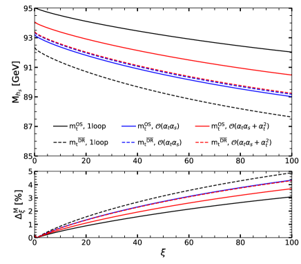
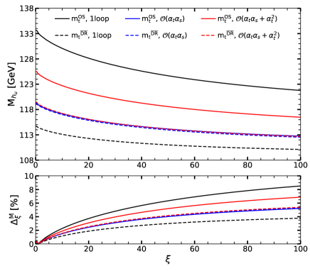
Figure 4: Upper Panel: The CP-even singlet-like (left) and the SM-like (right) Higgs boson masses as a function of the gauge parameter $\xi$ at the one-loop (black), two-loop ${\cal O}(\alpha_{t}\alpha_{s})$ (blue), two-loop ${\cal O}(\alpha_{t}\alpha_{s}+\alpha_{t}^{2})$ (red) level in the OS (solid lines) and the $\overline{\text{DR}}$ (dashed lines) scheme of the top/stop sector. Lower Panel: Absolute value of the relative $\xi$ dependence of the loop-corrected masses, defined as $\Delta^{M}_{\xi}=\absolutevalue{M_{x}(\xi)-M_{x}(\xi=1)}/M_{x}(\xi=1)$ ($x=h_{s},h_{u}$), in percent, as function of $\xi$. The color code in the lower plots is the same as in the upper plots.

We first vary the gauge parameter $\xi$ of the general $R_{\xi}$ gauge, which we set throughout the section $\xi_{W}=\xi_{Z}\equiv\xi$, while all other parameters are kept fixed. The masses of the $h_{s}$- and the $h_{u}$-like Higgs bosons depend significantly on $\xi$. All remaining Higgs bosons have masses larger than 600 GeV and show a very small gauge dependence. This is due to the fact that only the light Higgs bosons receive significant loop corrections. In Fig. 4, we show these dependences for the mass $M_{h_{s}}$ of the CP-even singlet-like Higgs boson in the upper left plot and for the mass $M_{h_{u}}$ of the SM-like Higgs boson in the upper right plot including one-loop (black lines), ${\cal O}(\alpha_{t}\alpha_{s})$ two-loop (blue lines) and ${\cal O}(\alpha_{t}\alpha_{s}+\alpha_{t}^{2})$ two-loop (red lines) corrections. These corrections are obtained for the OS (full lines) and $\overline{\text{DR}}$ (dashed lines) renormalization schemes of the top/stop sector. The two lower plots display the relative difference between the masses in general $R_{\xi}$ gauge and in the ’t Hooft–Feynman gauge $\xi=1$,

$$\Delta_{\xi}^{M}=\frac{\absolutevalue{M_{x}(\xi)-M_{x}(\xi=1)}}{M_{x}(\xi=1)},\quad\text{with}\quad x=h_{s},h_{u}\;,$$ (105)

as functions of $\xi$. Here $M_{x}$ denotes the loop-corrected mass value of the Higgs boson $x$ at a fixed loop order, calculated in general $R_{\xi}$ gauge ($M_{x}(\xi)$) and in the ’t Hooft–Feynman gauge ($M_{x}(\xi=1)$). We remind the reader that only the renormalized one-loop Higgs self-energies are calculated in general $R_{\xi}$ gauge and therefore depend on $\xi$, while the renormalized two-loop Higgs self-energies at order ${\cal O}(\alpha_{t}\alpha_{s})$ and ${\cal O}(\alpha_{t}^{2})$ do not depend on $\xi$ as they are computed in the gaugeless limit. Note that the tree-level masses for the $h_{s}$- and $h_{u}$-like Higgs bosons are 9.8 GeV and 91.38 GeV, respectively. The loop corrections to their masses are positive. From the plots, we can infer that the loop-corrected masses decrease with increasing $\xi$, which we chose to lie between 0 and 100. We can, however, increase $\xi$ to a larger value and find that for $\xi=1089$ the loop-corrected mass of the $h_{s}$-like Higgs boson becomes negative. In the lower plots, we see two different behaviors for the $h_{s}$- and $h_{u}$-like Higgs boson. The relative $\xi$ dependence is larger in the $\overline{\text{DR}}$ scheme than in the OS scheme for the loop-corrected $h_{s}$-like Higgs boson masses, while the behavior is opposite for the loop-corrected $h_{u}$-like Higgs boson masses. The inclusion of the two-loop corrections of order ${\cal O}(\alpha_{t}\alpha_{s})$ and ${\cal O}(\alpha_{t}^{2})$ changes $\Delta^{M}_{\xi}$ in an intricate way. The relative differences $\Delta_{\xi}^{M}$ in the OS and $\overline{\text{DR}}$ scheme, however, move closer to each other with the inclusion of the two-loop corrections.

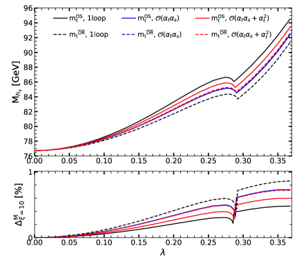
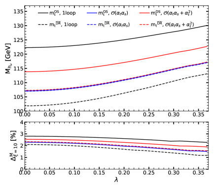
Figure 5: Analogous to Fig. 4, but $\lambda$ is varied while $\xi$ is kept fixed at $\xi=10$.

Next, we fix the value of $\xi$ to 10 and vary $\lambda$ and $\kappa$ at the same time to very small values ($10^{-5}$) while we keep the ratio $\lambda/\kappa$ constant. In this way we smoothly approach the MSSM limit, where the singlet and doublet Higgs bosons do not mix. In Fig. 5 we show the thus obtained loop-corrected masses of the $h_{s}$-like (left) and $h_{u}$-like (right) Higgs boson as function of $\lambda$. The line and color codes are the same as in Fig. 4. The lower plots show $\Delta^{M}_{\xi=10}$, i.e. the deviation of the $h_{s}$- and $h_{u}$-like masses, respectively, calculated for $\xi=10$ from the value obtained in the ’t Hooft–Feynman gauge.

As expected, when $\lambda$ and $\kappa$ are close to zero, the $h_{s}$-like Higgs boson decouples and the loop corrections to the $h_{s}$-like Higgs boson mass vanish in this limit. Therefore all lines in the left plots converge at the left endpoint where $\lambda\approx 0$. As we can see from Fig. 5 (right), the $\xi$ dependence of the SM-like loop-corrected Higgs boson masses does not vanish in the MSSM limit. For our chosen parameter point the relative deviation of the masses for $\xi=10$ and $\xi=1$ even slightly increases. The kink around $\lambda=0.29$ appears at the threshold where the loop-corrected $h_{s}$ mass is twice the tree-level $h_{s}$ mass.

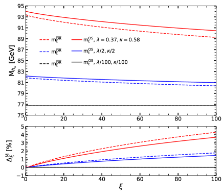
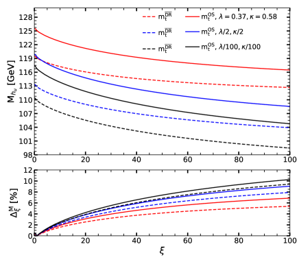
Figure 6: Upper panel: The CP-even singlet-like (left) and the $h_{u}$-like (right) Higgs boson masses at two-loop ${\cal O}(\alpha_{t}\alpha_{s}+\alpha_{t}^{2})$ level in the OS (solid lines) and the $\overline{\text{DR}}$ (dashed lines) scheme of the top/stop sector for $\lambda=0.37,\kappa=0.58$, i.e. the P1 values, (red), for half their values (blue) and for $\lambda/100$, $\kappa/100$ (black). Lower panel: Corresponding $\Delta^{M}_{\xi}$ in percent, as function of $\xi$.

In order to investigate the influence of the NMSSM-specific contributions to the mass corrections at ${\cal O}(\alpha_{t}\alpha_{s}+\alpha_{t}^{2})$ and their $\xi$ dependence we simultaneously vary the couplings $\lambda$ and $\kappa$ and show in Fig. 6 (upper) the two-loop masses of the singlet-like (left) and the $h_{u}$-like (right) Higgs bosons for the original values for $\lambda$ and $\kappa$ of the parameter point P1 (red lines), half their values (blue) and for $\lambda/100$, $\kappa/100$ (black) in the two renormalization schemes of the top/stop sector. In the left plot the black dashed and full lines lie on top of each other. The lower plots depict the corresponding relative $\xi$ dependence. For $h_{s}$ the two-loop corrected mass value and the $\xi$ dependence decrease with smaller values of the NMSSM-like couplings, as the singlet-like Higgs boson decouples from the spectrum. The $h_{u}$-like mass shows the expected behavior and decreases with smaller singlet admixtures. The relative $\xi$ dependence increases, however, for the chosen parameter point. The increasing contribution to the mass corrections for larger $\lambda$, $\kappa$ values from the $h_{u}-h_{s}$ admixture mixes with the doublet-like mass corrections and diminishes their gauge dependence.

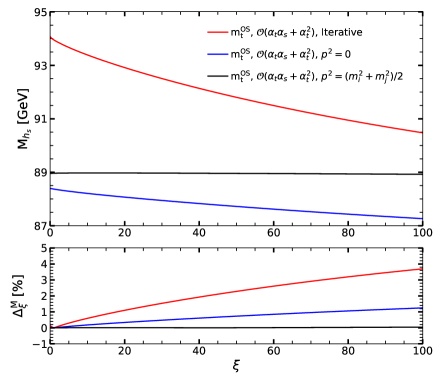
Figure 7: Upper Panel: The CP-even singlet-like (left) and the $h_{u}$-like (right) Higgs boson masses at two-loop ${\cal O}(\alpha_{t}\alpha_{s}+\alpha_{t}^{2})$ level in the OS scheme of the top/stop sector applying the iterative (red), the $R^{0}$- (blue) and the $R^{\text{mtree}}$-method (black). See text, for explanations. Lower Panel: Corresponding $\Delta^{M}_{\xi}$ in percent, as function of $\xi$.

The gauge dependence strongly depends on the chosen approach to determine the loop-corrected masses as we will show next. Figure 7 displays the mass corrections (upper plots) at ${\cal O}(\alpha_{t}\alpha_{s}+\alpha_{t}^{2})$ for OS renormalization in the top/stop sector and their relative $\xi$ dependence (lower plots) determined through the iterative method to extract the zeros of the determinant [26] (red lines) as well as when we apply the zero momentum approximation (’$R^{0}$-method’ called in the following, blue lines), cf. Eq. (33), and when the mass matrix is diagonalized at the arithmetic squared mass average (’$R^{\text{mtree}}$-method’, black lines), cf. Eqs. (35) and (36). The gauge dependence becomes very small for the latter in contrast to the two former methods. This is because of the fact that the dependence of the renormalized self-energy $\hat{\Sigma}_{h_{i}h_{j}}$ evaluated at the arithmetic squared mass average on the gauge parameter is small for $i$ being different from $j$ and vanishes completely for $i$ being identical to $j$. Their behavior as a function of $\xi$ depends on the difference between the tree-level mass and the squared momentum at which the mass matrix is diagonalized resulting in $\Delta^{M}_{\xi}$ values up to about 1% (4%) for the $R_{0}$-method (iterative method) for the $h_{s}$-like mass and 10% (7%) for the $h_{u}$-like mass when $\xi$ is varied up to values of 100.

4.3 Gauge Dependence of the Loop-Corrected Decay Width

In this section, we investigate the gauge dependence of the loop-corrected decay width computed in Sec. 3.

4.3.1 Individual Loop Contributions

We start with the study of the gauge dependence of the various components of the virtual one-loop correction, namely $\mathcal{M}^{\text{vert}},\mathcal{M}^{\text{ext},H^{\pm}},\mathcal{M}^{\text{ext},h}$, and finally of the complete virtual amplitude $\mathcal{M}^{\text{virt}}$, as defined in Sec. 3.2. We use the same parameter point as given in Eqs. (83) and (84).

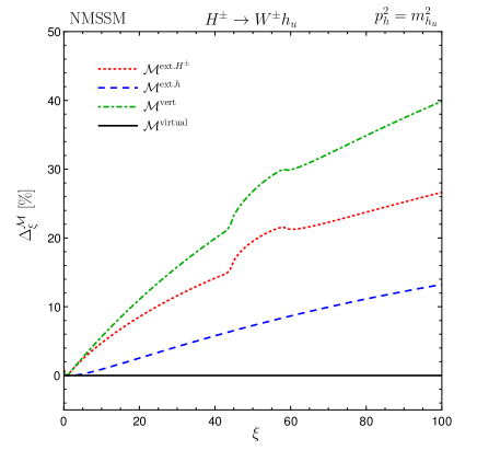
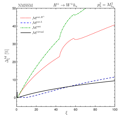
Figure 8: Gauge dependence of the virtual electroweak corrections to $H^{\pm}\to W^{\pm}h_{u}$, with $\mathcal{M}^{\text{ext},H^{\pm}}$ (dotted, red), $\mathcal{M}^{\text{ext},h}$ (blue, dashed), $\mathcal{M}^{\text{vert}}$ (green, dot-dashed) and $\mathcal{M}^{\text{virt}}$ (black, solid). Left plot: virtual corrections computed at strict one-loop order. Right plot: virtual corrections computed with the external momentum set to the loop-corrected neutral Higgs boson mass $p_{h}^{2}=M_{h_{u}}^{2}$. For details, we refer to the text.

In Fig. 8 we show the relative gauge dependence of the virtual amplitude and of its individual contributions for the electroweak loop correction to the decay $H^{\pm}\to W^{\pm}h_{u}$ as a function of the gauge parameter $\xi$, where the mostly $h_{u}$-like Higgs boson corresponds to the SM-like Higgs boson. We define the quantity $\Delta^{\cal M}_{\xi}$ to measure the gauge dependence of the amplitude ${\cal M}$, by

$$\Delta^{\cal M}_{\xi}=\frac{\absolutevalue{\mathcal{M}_{\xi}-\mathcal{M}_{\xi=1}}}{\absolutevalue{\mathcal{M}^{\text{virt}}_{\xi=1}}}\;,$$ (106)

where ${\cal M}_{\xi}$ with ${\cal M}\in\{\mathcal{M}^{\text{vert}},\mathcal{M}^{\text{ext},H^{\pm}},\mathcal{M}^{\text{ext},h},\mathcal{M}^{\text{virt}}\}$ denotes the amplitude in the general $R_{\xi}$ gauge and ${\cal M}_{\xi=1}$ the computed in the ’t Hooft–Feynman gauge $\xi=1$. Note that we normalize to ${\cal M}^{\text{virt}}$, i.e. to the sum of all contributions to the virtual corrections of the one-loop amplitude, at $\xi=1$. We choose to vary $\xi$ between 0 and 100 in order not to introduce new scales in the calculation (the Goldstone masses scale with $\sqrt{\xi}m_{\text{gauge}}$ where $m_{\text{gauge}}$ denotes the electroweak gauge boson masses). The individual components of the virtual corrections include their respective counterterms, such that the individual parts are UV-finite, but still IR-divergent. The IR divergence is regulated by a finite photon mass. The red (dotted) curve depicts the relative gauge dependence of the external leg corrections $\mathcal{M}^{\text{ext},H^{\pm}}$ to the charged Higgs boson, the blue one (dashed) is the corresponding curve for the external leg correction $\mathcal{M}^{\text{ext},h}$ to the outgoing neutral Higgs $h_{u}$, and the green (dot-dashed) curve depicts the relative gauge dependence of the vertex corrections $\mathcal{M}^{\text{vert}}$. Finally, the solid black curve shows the result for the total virtual correction $\mathcal{M}^{\text{virt}}$. In the left plot of Fig. 8, we show these curves for the strict one-loop calculation as described in Sec. 3.2. This means that the external leg corrections to $h_{u}$ are accounted for diagrammatically using Eq. (2.2), as opposed to using the resummed $\mathbf{Z}$ matrix. Moreover, we use the tree-level mass $m_{h_{u}}$ for the external momentum such that $p_{h}^{2}=m_{h_{u}}^{2}$. Here and in the following plots we use the mixing matrix that diagonalizes the tree-level mass matrices in the computation of the couplings as otherwise the result will not be UV-finite. In this strict one-loop computation, the virtual corrections are gauge independent, as can be checked explicitly numerically, cf. the solid black curve of Fig. 8 (left): while each individual component of the virtual correction is gauge dependent, their sum, resulting in $\mathcal{M}^{\text{virt}}$, is gauge independent. Actually, the relative gauge dependences of the external leg contributions to the charged and the neutral Higgs mass, ${\cal M}^{\text{ext},H^{\pm}}$ and ${\cal M}^{\text{ext},h}$, and the ones of the vertex corrections, ${\cal M}^{\text{vert}}$, come with opposite sign (not visible from the plot as we show the absolute values). The reason for the kinks in the red (dotted) and green (dot-dashed) curves is the following. The masses of the Goldstone bosons depend on the gauge parameter $\xi$, and these kinks occur when a production threshold for the Goldstone boson is reached, i.e. at the points

$$m_{H^{\pm}}=\sqrt{\xi}M_{W}+m_{h_{j}}\quad\text{and}\quad m_{H^{\pm}}=\sqrt{\xi}M_{Z}+m_{a_{j}}\,.$$ (107)

In Fig. 8 (right), we investigate how this gauge independence of the strict one-loop computation changes when we apply the improved one-loop computation as defined in Sec. 3.4 ’Step 1’ that we denoted ’off-shell’. The means, we use loop-corrected masses for the external leg corrections to the neutral Higgs boson $h_{u}$, i.e. we set $p_{h}^{2}=M_{h_{u}}^{2}$. Note, however, that the $\mathbf{Z}$ matrix is evaluated at pure one-loop order, as defined in Eq. (2.2). The masses are calculated at ${\cal O}(\alpha_{t}\alpha_{s}+\alpha_{t}^{2})$ for OS renormalization in the top/stop sector by NMSSMCALC in general $R_{\xi}$ gauge as described in subsection 2.2. Going from the strict one-loop calculation to the ’off-shell’ one, we see that the dependence of the individual components of the virtual corrections on the gauge parameter $\xi$ changes, such that their sum $\mathcal{M}^{\text{virt}}$ (solid, black curve) is no longer gauge independent. The overall gauge dependence does not cancel any more, as we move away from the strict fixed-order calculation and include partial higher-order effects coming from the loop-corrected Higgs mass $M_{h_{u}}^{2}$, such that with increasing $\xi$ values, the NLO amplitude becomes arbitrarily large. The relative change of the total virtual amplitude is of up to ${\cal O}(10\%)$ for $\xi$ values up to 100.

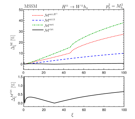
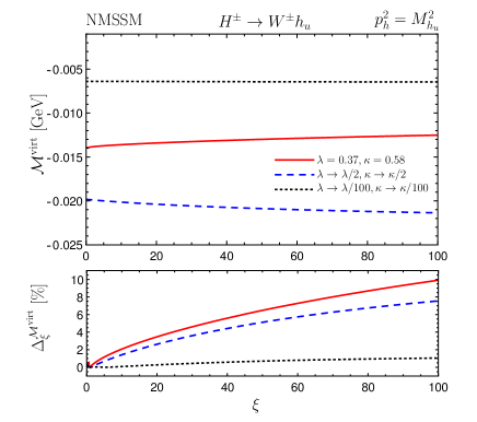
Figure 9: Left: Gauge dependence of the virtual electroweak corrections to $H^{\pm}\to W^{\pm}h_{u}$ in the MSSM-limit, using loop-corrected masses for the external neutral Higgs boson $p_{h}^{2}=M_{h_{u}}^{2}$ calculated in general $R_{\xi}$ gauge. The color and line code is the same as in Fig. 8. Lower panel: Gauge dependence of $\mathcal{M}^{\text{virt}}$ with the vertical axis zoomed-in Right: ${\cal M}^{\text{virt}}$ as a function of $\xi$ (upper) and its relative gauge dependence (lower) for $\lambda=0.37$, $\kappa=0.58$ (parameter point P1, red/full lines) and their variation to half their values (blue/dashed lines) and to $\lambda/100$, $\kappa/100$ (black/dotted lines).

In Fig. 9 (left), the curves corresponding to the right plot of Fig. 8 are plotted in the MSSM limit of the chosen parameter point. This limit is taken by setting $\lambda,\kappa\to 0$ and keeping the ratio $\lambda/\kappa$ constant (actually $\lambda,\kappa={\cal O}(10^{-8})$). From Fig. 9 we see that in the MSSM limit the resulting gauge dependence of $\mathcal{M}^{\text{virt}}$ has a numerically small effect. It varies up to 0.7%, although we are using gauge-dependent loop-corrected masses for the external momentum $p_{h}^{2}=M_{h_{u}}^{2}$. This is illustrated once again in the right plot of the figure, where we show ${\cal M}^{\text{virt}}$ and its relative gauge dependence alone for the chosen parameter point (red) and after varying $\lambda$ and $\kappa$ to half their values (blue) and to $\lambda/100$ and $\kappa/100$ (black). The relative gauge dependence decreases successively from 10% to 1% at $\xi=100$. While the gauge dependence of the masses increases in the MSSM limit for our chosen parameter point the opposite is hence the case for the loop corrections to the decay. This again shows that the singlet admixtures play an important role for the gauge dependence of the parameters and observables and do not follow a simple law.

4.3.2 The Complete Loop-Corrected Decay Width

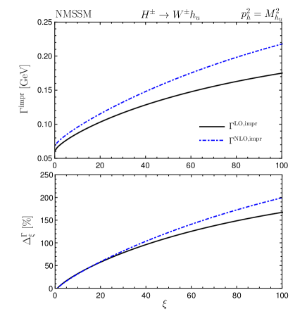
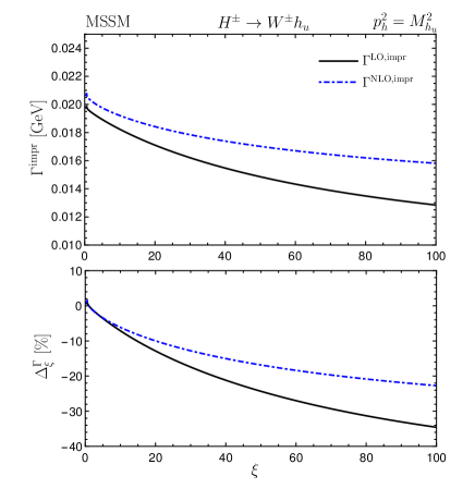
Figure 10: Parameter point P1: gauge dependence of the LO and NLO decay widths in the NMSSM (left) and its MSSM limit (right). $\Gamma^{\text{impr}}$ depicts widths calculated using the resummed $\mathbf{Z}$ matrix defined in Eq. (37). The upper panels show the gauge dependence of the LO (black, solid) and NLO (blue, dot-dashed) widths. In the lower panels we display the relative gauge dependence of the LO and NLO widths.

In the following, we study for the parameter point P1 the gauge dependence of the complete loop-corrected partial decay width of the decay $H^{\pm}\to W^{\pm}h_{u}$. In the upper plots of Fig. 10, the black (solid) curve shows, as a function of $\xi$, the improved LO decay width for $H^{\pm}\to W^{\pm}h_{u}$, i.e. we apply Eq. (61) as denoted with ’Step 2’ in Sec. 3.4. This means that we set the external momentum to the loop-corrected Higgs boson mass $M_{h_{u}}$, $p_{h}^{2}=M_{h_{u}}^{2}$, which is calculated at ${\cal O}(\alpha_{t}\alpha_{s}+\alpha_{t}^{2})$ with OS renormalization in the top/stop sector. Additionally, we include in the external-leg corrections to the neutral Higgs boson the resummed $\mathbf{Z}$ matrix defined in Eq. (37) in order to ensure the correct OS properties. The blue (dot-dashed) curve displays the corresponding improved NLO width, given by Eq. (64). The left plots are for the NMSSM parameter point P1, whereas the right plots are for the MSSM limit of the same benchmark point. The NMSSM widths show a stronger dependence on $\xi$ than the ones in the MSSM limit (note that the scales of the two plots are different). In the lower plots we show the relative gauge dependence of the LO and NLO widths, respectively, as a function of $\xi$, as defined by

$$\Delta^{\Gamma}_{\xi}=\frac{\Gamma_{\xi}-\Gamma_{\xi=1}}{\Gamma_{\xi=1}}\;.$$ (108)

Here $\Gamma_{\xi}$ denotes the decay width calculated in general $R_{\xi}$ gauge at fixed loop order, i.e. $\Gamma^{\text{LO, impr}}$ or $\Gamma^{\text{NLO, impr}}$, and $\Gamma_{\xi=1}$ the width calculated in the ’t Hooft–Feynman gauge. In the NMSSM the relative gauge dependence is larger for the NLO width than for the LO one while in the MSSM, where the singlet admixture vanishes, the opposite is the case. For the complete NLO width of scenario P1 the relative corrections $\Delta^{\Gamma}_{\xi}$ can become as large as 200% for $\xi=100$. Such a strong gauge dependence is clearly unacceptable for making meaningful predictions for the decay widths. For phenomenological investigations, on the other hand, the interesting quantity is the branching ratio. In order to make meaningful predictions, this requires the inclusion of the electroweak corrections to all other charged Higgs boson decays, so that the total width entering the branching ratio is computed at higher order in the electroweak corrections. This is beyond the scope of the present paper and left for future work. Even if one argues not to introduce new mass scales in the process and to remain below $\xi$ values of 100 the $\xi$ dependence is large, in particular it is far beyond the relative size of the loop corrections which is about 11% for $\xi=1$. In the MSSM limit, depicted in the right plot of Fig. 10, the relative gauge dependence is smaller with values of up to about 20% for $\xi=100$.

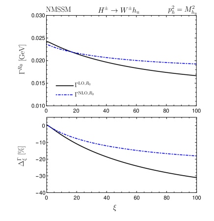
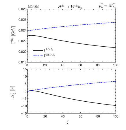
Figure 11: Analogous to Fig. 10, but using the $R^{0}$-method instead of the iterative approach to extract the loop-corrected masses and mixing matrix.

In Fig. 11, we show the corresponding curves analogous to Fig. 10, however now using the $R^{0}$ method to extract the loop-corrected mass values and mixing matrix. The LO and NLO widths are then calculated by applying Eqs. (59) to (63), but with the ${\bf Z}$ matrix replaced by the $R^{0}$ matrix, defined in Eq. (33). We denote the corresponding widths with the superscript $R^{0}$ as $\Gamma^{R^{0}}$. Figure 12 shows the corresponding results if the masses are extracted at the arithmetic squared mass average such that the ${\bf Z}$ matrix is replaced by the $R^{\text{mtree}}$ matrix, defined in Eqs. (35,36). The corresponding widths are denoted by the superscript $R^{\text{mtree}}$.

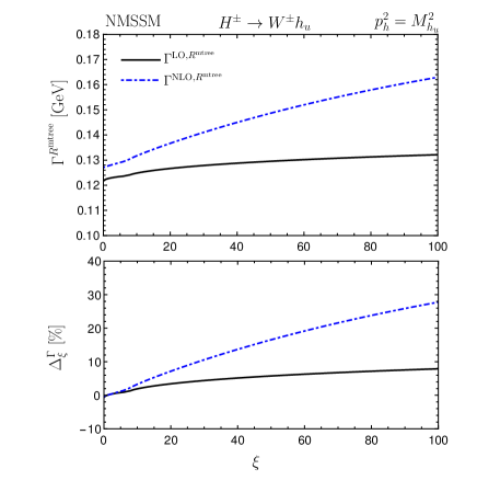
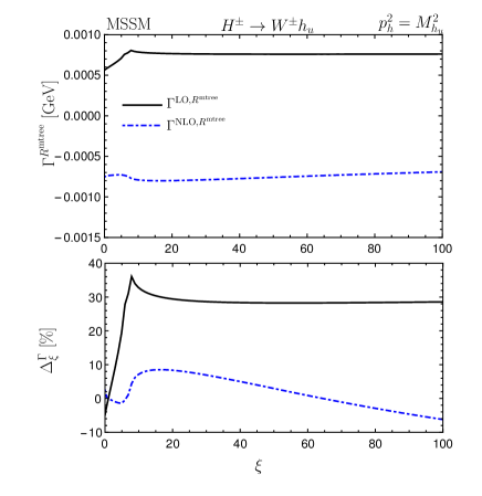
Figure 12: Same as Fig. 10, but using the $R^{\text{mtree}}$-method instead of the iterative approach to extract the loop-corrected masses and mixing matrix.

The comparison of Figs. 11 and 12 with Fig. 10 shows that for this parameter point the gauge dependence is smallest in the $R^{0}$ approximation. The relative change of the complete NLO width with $\xi$ compared to its value for $\xi=1$, i.e. $\Delta_{\xi}^{\Gamma}$, is about -18% for $\xi=100$, while in the $R^{\text{mtree}}$ approximation it is about +28%, which is still smaller than if the ${\bf Z}$ matrix is applied. The corresponding values in the MSSM limit are 6.5% ($R^{0}$) and -6% ($R^{\text{mtree}}$). The method of extracting the mixing matrix elements has a strong influence on the $\xi$ dependence of the NLO width and also on the sign of this $\xi$ dependence. For the parameter point P1 the $h_{u}$-like Higgs boson has a strong singlet admixture. From previous analyses [49, 51], we know already that the mixing matrix elements are then very sensitive to changes in the approximation of the loop calculation. Since the mixing matrix elements enter the Higgs couplings, the computed observables, in this case the decay width, become very sensitive to the applied approximation. This is confirmed by our results on the $\xi$ dependence but also by the values of the widths themselves for the various approximations.

Overall, we found that the gauge dependence of the loop-corrected mass of the external neutral Higgs boson has a much smaller influence on the gauge dependence of the NLO width than the matrix that is used to set the external Higgs boson OS. The strength of this effect sensitively depends on the chosen parameter set, as can be inferred from Fig. 13. The figure displays the partial decay widths of the decay $H^{\pm}\to W^{\pm}h_{u}$ (left plot) and $H^{\pm}\to W^{\pm}h_{s}$ (right plot) both at LO and NLO as a function of $\tan\beta$. All other parameter values are fixed to those of scenario P1. Shown are the results for the pure LO and strict one-loop width (black lines) and the ones when we calculate the improved LO and NLO widths applying the ${\bf Z}$ matrix (red) and the $R_{0}$ matrix (green). The lower plots show the corresponding $K$ factors, defined as the ratio of the NLO width and its corresponding LO width

$$K=\frac{\Gamma^{\text{NLO}}}{\Gamma^{\text{LO}}}\;.$$ (109)

As can be inferred from the left plot, the value of the decay width $\Gamma(H^{\pm}\to W^{\pm}h_{u})$ strongly depends on the applied approximation for our chosen parameter point, i.e. for $\tan\beta=3.11$, while the $K$ factor is approximately the same for the improved widths, with a value around 1.1. The $K$ factor for the pure one-loop result largely differs from the improved ones as it does not take into account any resummation of higher orders. For values of $\tan\beta$ between about 3.26 and 3.52 the improved NLO results are rather close, but differ otherwise. In the singlet-like final state shown in Fig. 13 (right), i.e. $\Gamma(H^{\pm}\to W^{\pm}h_{s})$, the $K$ factors for the improved widths differ by less than 5% over the whole scanned range.

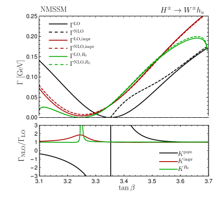
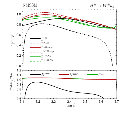
Figure 13: Parameter point P1: partial decay width of the decay $H^{\pm}\to W^{\pm}h_{u}$ (left) and $H^{\pm}\to W^{\pm}h_{s}$ (right) at LO (full) and NLO (dashed) at strict LO and one-loop order (black), in the improved approach applying the ${\bf Z}$ matrix (red) and the $R_{0}$ matrix (green), as a function of $\tan\beta$. Lower panels: corresponding $K$ factors.

4.4 Analysis for Scenario P2

In order to further investigate the impact of the gauge dependence, we analyze the gauge dependence of the Higgs boson masses and the charged Higgs decay widths for a second parameter point, P2, defined in Eqs. (85) and (86). We summarize the Higgs boson masses obtained in the OS renormalization scheme of the top/stop sector in Table 4 and in the $\overline{\text{DR}}$ scheme in Table 5, at tree level, at one-loop level and at two-loop level including the ${\cal O}(\alpha_{t}\alpha_{s})$ and the ${\cal O}(\alpha_{t}\alpha_{s}+\alpha_{t}^{2})$ corrections, respectively. We have deliberately chosen this scenario in which the $h_{u}$-like Higgs boson is the lightest state with mass around 125 GeV at ${\cal O}(\alpha_{t}\alpha_{s}+\alpha_{t}^{2})$ in the OS renormalization scheme of the top/stop sector while the CP-even singlet-like Higgs boson is the second-lightest state with mass around 433 GeV. In this scenario we analyze only the mass of the $h_{u}$-like Higgs boson since only its mass is affected substantially by the change of the gauge parameter $\xi$. We present in Fig. 14 the $h_{u}$-like Higgs boson mass as function of $\xi$. The left plot shows its two-loop mass at ${\cal O}(\alpha_{t}\alpha_{s}+\alpha_{t}^{2})$ for OS (full) and $\overline{\mbox{DR}}$ (dashed) renormalization in the top/stop sector for three different singlet admixtures. This means we start with the $\lambda$ and $\kappa$ values of our original scenario P2 (red lines) and compare with the results when we take half (blue lines) and 1/100 their values (black lines), where the latter means that we are close to the MSSM limit. As can be inferred from the plot, the gauge dependence $\Delta^{M}_{\xi}$ shown in the lower plot is only mildly dependent on the renormalization scheme and on the singlet admixture, and amounts up to values of about 7 to 8 % at $\xi=100$.

	$h_{1}/{H_{1}}$	$h_{2}/{H_{2}}$	$h_{3}/{H_{3}}$	$h_{4}/{H_{4}}$	$h_{5}/{H_{5}}$
tree-level	85.43	437.27	581.25	986.77	989.68
main component	$h_{u}$	$h_{s}$	$a$	$a_{s}$	$h_{d}$
one-loop	133.59	433.79	577.39	989.71	986.69
main component	$h_{u}$	$h_{s}$	$a$	$a_{s}$	$h_{d}$
two-loop ${\cal O}(\alpha_{t}\alpha_{s})$	118.38	433.76	577.42	989.61	986.7
main component	$h_{u}$	$h_{s}$	$a$	$a_{s}$	$h_{d}$
two-loop ${\cal O}(\alpha_{t}\alpha_{s}+\alpha_{t}^{2})$	125.03	433.76	577.42	989.66	986.7
main component	$h_{u}$	$h_{s}$	$a$	$a_{s}$	$h_{d}$

Table 4: P2: mass values in GeV and main components of the neutral Higgs bosons at tree level, one-loop level, two-loop ${\cal O}(\alpha_{t}\alpha_{s})$ level and at two-loop ${\cal O}(\alpha_{t}\alpha_{s}+\alpha_{t}^{2})$ level obtained by using OS renormalization in the top/stop sector.

	$h_{1}/{H_{1}}$	$h_{2}/{H_{2}}$	$h_{3}/{H_{3}}$	$h_{4}/{H_{4}}$	$h_{5}/{H_{5}}$
tree-level	85.43	437.27	581.25	986.77	989.68
main component	$h_{u}$	$h_{s}$	$a$	$a_{s}$	$h_{d}$
one-loop	113.9	433.75	577.43	989.55	986.65
main component	$h_{u}$	$h_{s}$	$a$	$a_{s}$	$h_{d}$
two-loop ${\cal O}(\alpha_{t}\alpha_{s})$	118.4	433.76	577.42	989.56	986.64
main component	$h_{u}$	$h_{s}$	$a$	$a_{s}$	$h_{d}$
two-loop ${\cal O}(\alpha_{t}\alpha_{s}+\alpha_{t}^{2})$	118.86	433.76	577.42	989.57	986.64
main component	$h_{u}$	$h_{s}$	$a$	$a_{s}$	$h_{d}$

Table 5: P2: mass values in GeV and main components of the neutral Higgs bosons at tree level, one-loop level, two-loop ${\cal O}(\alpha_{t}\alpha_{s})$ level and at two-loop ${\cal O}(\alpha_{t}\alpha_{s}+\alpha_{t}^{2})$ level obtained by using $\overline{\text{DR}}$ renormalization in the top/stop sector.

In the right plot of Fig. 14 we show the $\xi$ dependence of $M_{h_{u}}$ when we apply different approximations to determine the loop-corrected Higgs mass eigenstates with OS renormalization of the top/stop sector, namely through the iterative method (red line), by applying the rotation matrix $R^{0}$ to the mass matrix in the zero momentum approximation (blue), or finally by applying $R^{\text{mtree}}$ to the mass matrix evaluated at its arithmetic squared mass average (black). The $\xi$ dependence of the iterative and the zero momentum procedure is about the same, with $\Delta^{M}_{\xi}$ amounting to 8 and 9%, respectively, at $\xi=100$. For the arithmetic squared mass average method, however, we again find that the $\xi$ dependence is very small. Overall, the gauge dependence of the $h_{u}$-like mass in scenario P1 is larger than in P2.

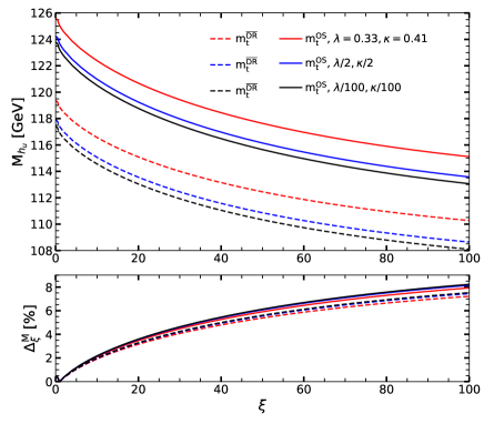
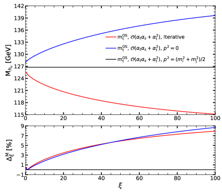
Figure 14: Left: The $h_{u}$-like Higgs boson masses as a function of $\xi$ at two-loop ${\cal O}(\alpha_{t}\alpha_{s}+\alpha_{t}^{2})$ level in the OS (solid lines) and the $\overline{\text{DR}}$ (dashed lines) scheme of the top/stop sector for scenario P2, i.e. $\lambda=0.33,\kappa=0.41$ (red line), for half their values (blue) and for $\lambda/100$, $\kappa/100$ (black). Right: The $h_{u}$-like Higgs boson mass of scenario P2 as a function of $\xi$ by applying iterative (red), the $R^{0}$ (blue) and the $R^{\text{mtree}}$-method (black). Lower panels: The corresponding $\Delta^{M}_{\xi}$ values in percent, as a function of $\xi$.

Figure 15 depicts the gauge dependence of the partial widths of the decays $H^{\pm}\to W^{\pm}h_{u}$ (left) and $H^{\pm}\to W^{\pm}h_{s}$ (right) at LO (full lines) and NLO (dashed lines) by applying in Eqs. (61) and (64), respectively, the three different approximations for the matrices that diagonalize the corresponding loop-corrected mass matrices, namely the ${\bf Z}$ matrix (red), $R^{0}$ (blue) and $R^{\text{mtree}}$ (black). The corresponding decay widths are denoted by the superscripts ’impr’, ’$R^{0}$’ and ’$R^{\text{mtree}}$’. The lower panels display the corresponding $\Delta_{\xi}^{\Gamma}$ values. The inspection of the plots shows that the $\xi$ dependence of the NLO widths not always decreases compared to the LO one. Moreover, there is no pattern for the two decays that allows to decide which of the three approximations induces the smallest gauge dependence in the NLO widths. A closer investigation reveals that the mixing between $h_{u}$ and $h_{d}$ is responsible for the gauge dependence of $H^{\pm}\to W^{\pm}h_{u}$ and the mixing between $h_{s}$ and $h_{d}$ for the one in $H^{\pm}\to W^{\pm}h_{s}$. Overall, however, the gauge dependence of the partial widths is much smaller than for the parameter point P1, with maximum values of $\Delta_{\xi}^{\Gamma}$ around $-22\%$ for $H^{\pm}\to W^{\pm}h_{u}$ (for $\Gamma^{\text{NLO},\text{impr}}$) and 14% for $H^{\pm}\to W^{\pm}h_{s}$ (for $\Gamma^{\text{LO},R^{\text{mtree}}}$). The relative NLO corrections at $\xi=1$ amount to -20% (for $\Gamma^{\text{impr}}$) for the former and to -12% for the latter decay (for $\Gamma^{R^{\text{mtree}}}$), however, so that the gauge dependence is of the order of the loop correction.

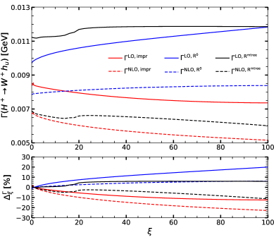
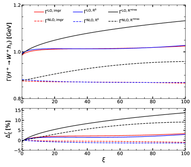
Figure 15: P2: Decay widths for $H^{\pm}\to W^{\pm}h_{u}$ (left uppper plot) and $H^{\pm}\to W^{\pm}h_{s}$ (right uppper plot) as functions of $\xi$ using the iterative (red), the $R^{0}$ (blue) and the $R^{\text{mtree}}$ method (black). Lower panels: Corresponding $\Delta^{\Gamma}_{\xi}$ in percent, as function of $\xi$.

5 Conclusions

In this paper we investigated the influence of the gauge parameter both on the higher-order corrections to the NMSSM Higgs boson masses and the partial decay width of $H^{\pm}\to W^{\pm}h_{i}$, calculated in general $R_{\xi}$ gauge. The gauge dependence enters through the mixing of loop orders: for the masses, this happens due to the application of an iterative method to determine the loop-corrected mass values. This is transferred to the decay width as phenomenology requires the inclusion of the mass corrections to the external Higgs bosons in order to match the experimentally measured values. These are calculated up to two-loop order including higher-order terms through the application of the iterative procedure. Gauge dependence then enters the process through different mechanisms. On the one hand there is a mismatch between the use of tree-level masses in the propagators of the internal lines and in the Higgs-Goldstone boson couplings appearing in the computation of the loops, and the use of the higher-order-corrected Higgs mass for the external Higgs bosons. The latter prevents the cancelation of IR divergences when adding up the virtual and real corrections. While this can be cured by an appropriate adaption of the involved couplings, the second source of the gauge dependences persists: it stems from the resummation of higher orders that enters both through the external Higgs boson mass and the mixing matrix applied to set the external Higgs boson OS. The latter has a particularly large impact as we found by applying different approximations to determine the higher-order masses and mixing matrix elements. The relative gauge dependence can then largely exceed the relative size of the loop correction itself, so that for the interpretation of the results the specification of the used gauge is crucial. By analyzing different parameter sets, we found that the impact of the gauge dependence depends on the chosen parameter point and can vary substantially depending on the applied parameter set.

References

- [1] ATLAS collaboration, G. Aad et al., Observation of a new particle in the search for the Standard Model Higgs boson with the ATLAS detector at the LHC, Phys. Lett. B716 (2012) 1–29, [1207.7214].
- [2] CMS collaboration, S. Chatrchyan et al., Observation of a New Boson at a Mass of 125 GeV with the CMS Experiment at the LHC, Phys. Lett. B716 (2012) 30–61, [1207.7235].
- [3] R. Barbieri, S. Ferrara and C. A. Savoy, Gauge Models with Spontaneously Broken Local Supersymmetry, Phys.Lett. B119 (1982) 343.
- [4] M. Dine, W. Fischler and M. Srednicki, A Simple Solution to the Strong CP Problem with a Harmless Axion, Phys.Lett. B104 (1981) 199.
- [5] J. R. Ellis, J. Gunion, H. E. Haber, L. Roszkowski and F. Zwirner, Higgs Bosons in a Nonminimal Supersymmetric Model, Phys.Rev. D39 (1989) 844.
- [6] M. Drees, Supersymmetric Models with Extended Higgs Sector, Int.J.Mod.Phys. A4 (1989) 3635.
- [7] U. Ellwanger, M. Rausch de Traubenberg and C. A. Savoy, Particle spectrum in supersymmetric models with a gauge singlet, Phys.Lett. B315 (1993) 331–337, [hep-ph/9307322].
- [8] U. Ellwanger, M. Rausch de Traubenberg and C. A. Savoy, Higgs phenomenology of the supersymmetric model with a gauge singlet, Z.Phys. C67 (1995) 665–670, [hep-ph/9502206].
- [9] U. Ellwanger, M. Rausch de Traubenberg and C. A. Savoy, Phenomenology of supersymmetric models with a singlet, Nucl.Phys. B492 (1997) 21–50, [hep-ph/9611251].
- [10] T. Elliott, S. King and P. White, Unification constraints in the next-to-minimal supersymmetric standard model, Phys.Lett. B351 (1995) 213–219, [hep-ph/9406303].
- [11] S. King and P. White, Resolving the constrained minimal and next-to-minimal supersymmetric standard models, Phys.Rev. D52 (1995) 4183–4216, [hep-ph/9505326].
- [12] F. Franke and H. Fraas, Neutralinos and Higgs bosons in the next-to-minimal supersymmetric standard model, Int.J.Mod.Phys. A12 (1997) 479–534, [hep-ph/9512366].
- [13] M. Maniatis, The Next-to-Minimal Supersymmetric extension of the Standard Model reviewed, Int. J. Mod. Phys. A25 (2010) 3505–3602, [0906.0777].
- [14] U. Ellwanger, C. Hugonie and A. M. Teixeira, The Next-to-Minimal Supersymmetric Standard Model, Phys. Rept. 496 (2010) 1–77, [0910.1785].
- [15] K. E. Williams and G. Weiglein, Precise predictions for decays in the complex MSSM, Phys. Lett. B660 (2008) 217–227, [0710.5320].
- [16] A. C. Fowler and G. Weiglein, Precise Predictions for Higgs Production in Neutralino Decays in the Complex MSSM, JHEP 01 (2010) 108, [0909.5165].
- [17] K. E. Williams, H. Rzehak and G. Weiglein, Higher order corrections to Higgs boson decays in the MSSM with complex parameters, Eur. Phys. J. C71 (2011) 1669, [1103.1335].
- [18] R. Benbrik, M. Gomez Bock, S. Heinemeyer, O. Stal, G. Weiglein and L. Zeune, Confronting the MSSM and the NMSSM with the Discovery of a Signal in the two Photon Channel at the LHC, Eur. Phys. J. C72 (2012) 2171, [1207.1096].
- [19] P. Gonzalez, S. Palmer, M. Wiebusch and K. Williams, Heavy MSSM Higgs production at the LHC and decays to WW,ZZ at higher orders, Eur. Phys. J. C73 (2013) 2367, [1211.3079].
- [20] D. T. Nhung, M. Muhlleitner, J. Streicher and K. Walz, Higher Order Corrections to the Trilinear Higgs Self-Couplings in the Real NMSSM, JHEP 11 (2013) 181, [1306.3926].
- [21] M. D. Goodsell, S. Liebler and F. Staub, Generic calculation of two-body partial decay widths at the full one-loop level, Eur. Phys. J. C77 (2017) 758, [1703.09237].
- [22] F. Domingo, P. Drechsel and S. Paßehr, On-Shell neutral Higgs bosons in the NMSSM with complex parameters, Eur. Phys. J. C77 (2017) 562, [1706.00437].
- [23] F. Domingo, S. Heinemeyer, S. Paßehr and G. Weiglein, Decays of the neutral Higgs bosons into SM fermions and gauge bosons in the -violating NMSSM, Eur. Phys. J. C78 (2018) 942, [1807.06322].
- [24] J. Baglio, T. N. Dao and M. Mühlleitner, One-Loop Corrections to the Two-Body Decays of the Neutral Higgs Bosons in the Complex NMSSM, 1907.12060.
- [25] ATLAS, CMS collaboration, G. Aad et al., Combined Measurement of the Higgs Boson Mass in Collisions at and 8 TeV with the ATLAS and CMS Experiments, Phys. Rev. Lett. 114 (2015) 191803, [1503.07589].
- [26] K. Ender, T. Graf, M. Muhlleitner and H. Rzehak, Analysis of the NMSSM Higgs Boson Masses at One-Loop Level, Phys. Rev. D85 (2012) 075024, [1111.4952].
- [27] T. Graf, R. Grober, M. Muhlleitner, H. Rzehak and K. Walz, Higgs Boson Masses in the Complex NMSSM at One-Loop Level, JHEP 10 (2012) 122, [1206.6806].
- [28] M. Mühlleitner, D. T. Nhung, H. Rzehak and K. Walz, Two-loop contributions of the order to the masses of the Higgs bosons in the CP-violating NMSSM, JHEP 05 (2015) 128, [1412.0918].
- [29] T. N. Dao, R. Gröber, M. Krause, M. Mühlleitner and H. Rzehak, Two-Loop Corrections to the Neutral Higgs Boson Masses in the CP-Violating NMSSM, 1903.11358.
- [30] M. Mühlleitner, D. T. Nhung and H. Ziesche, The order corrections to the trilinear Higgs self-couplings in the complex NMSSM, JHEP 12 (2015) 034, [1506.03321].
- [31] D. J. Miller, R. Nevzorov and P. M. Zerwas, The Higgs sector of the next-to-minimal supersymmetric standard model, Nucl. Phys. B681 (2004) 3–30, [hep-ph/0304049].
- [32] W. Siegel, Supersymmetric Dimensional Regularization via Dimensional Reduction, Phys.Lett. B84 (1979) 193.
- [33] D. Stockinger, Regularization by dimensional reduction: consistency, quantum action principle, and supersymmetry, JHEP 0503 (2005) 076, [hep-ph/0503129].
- [34] U. Ellwanger, Radiative corrections to the neutral Higgs spectrum in supersymmetry with a gauge singlet, Phys.Lett. B303 (1993) 271–276, [hep-ph/9302224].
- [35] T. Elliott, S. King and P. White, Supersymmetric Higgs bosons at the limit, Phys.Lett. B305 (1993) 71–77, [hep-ph/9302202].
- [36] T. Elliott, S. King and P. White, Squark contributions to Higgs boson masses in the next-to-minimal supersymmetric standard model, Phys.Lett. B314 (1993) 56–63, [hep-ph/9305282].
- [37] T. Elliott, S. King and P. White, Radiative corrections to Higgs boson masses in the next-to-minimal supersymmetric Standard Model, Phys.Rev. D49 (1994) 2435–2456, [hep-ph/9308309].
- [38] P. Pandita, Radiative corrections to the scalar Higgs masses in a nonminimal supersymmetric Standard Model, Z.Phys. C59 (1993) 575–584.
- [39] S. Ham, J. Kim, S. Oh and D. Son, The Charged Higgs boson in the next-to-minimal supersymmetric standard model with explicit CP violation, Phys.Rev. D64 (2001) 035007, [hep-ph/0104144].
- [40] S. Ham, S. Oh and D. Son, Neutral Higgs sector of the next-to-minimal supersymmetric standard model with explicit CP violation, Phys.Rev. D65 (2002) 075004, [hep-ph/0110052].
- [41] S. Ham, Y. Jeong and S. Oh, Radiative CP violation in the Higgs sector of the next-to-minimal supersymmetric model, hep-ph/0308264.
- [42] K. Funakubo and S. Tao, The Higgs sector in the next-to-MSSM, Prog.Theor.Phys. 113 (2005) 821–842, [hep-ph/0409294].
- [43] U. Ellwanger and C. Hugonie, Yukawa induced radiative corrections to the lightest Higgs boson mass in the NMSSM, Phys.Lett. B623 (2005) 93–103, [hep-ph/0504269].
- [44] S. Ham, S. Kim, S. Oh and D. Son, Higgs bosons of the NMSSM with explicit CP violation at the ILC, Phys.Rev. D76 (2007) 115013, [0708.2755].
- [45] G. Degrassi and P. Slavich, On the radiative corrections to the neutral Higgs boson masses in the NMSSM, Nucl.Phys. B825 (2010) 119–150, [0907.4682].
- [46] K. Cheung, T.-J. Hou, J. S. Lee and E. Senaha, The Higgs Boson Sector of the Next-to-MSSM with CP Violation, Phys.Rev. D82 (2010) 075007, [1006.1458].
- [47] F. Staub, W. Porod and B. Herrmann, The Electroweak sector of the NMSSM at the one-loop level, JHEP 1010 (2010) 040, [1007.4049].
- [48] M. D. Goodsell, K. Nickel and F. Staub, Two-loop corrections to the Higgs masses in the NMSSM, Phys. Rev. D91 (2015) 035021, [1411.4665].
- [49] F. Staub, P. Athron, U. Ellwanger, R. Gröber, M. Mühlleitner, P. Slavich et al., Higgs mass predictions of public NMSSM spectrum generators, Comput. Phys. Commun. 202 (2016) 113–130, [1507.05093].
- [50] P. Drechsel, L. Galeta, S. Heinemeyer and G. Weiglein, Precise Predictions for the Higgs-Boson Masses in the NMSSM, Eur. Phys. J. C77 (2017) 42, [1601.08100].
- [51] P. Drechsel, R. Gröber, S. Heinemeyer, M. M. Muhlleitner, H. Rzehak and G. Weiglein, Higgs-Boson Masses and Mixing Matrices in the NMSSM: Analysis of On-Shell Calculations, Eur. Phys. J. C77 (2017) 366, [1612.07681].
- [52] M. D. Goodsell and F. Staub, The Higgs mass in the CP violating MSSM, NMSSM, and beyond, Eur. Phys. J. C77 (2017) 46, [1604.05335].
- [53] J. Fleischer and F. Jegerlehner, Radiative Corrections to Higgs Decays in the Extended Weinberg-Salam Model, Phys. Rev. D23 (1981) 2001–2026.
- [54] A. Denner, L. Jenniches, J.-N. Lang and C. Sturm, Gauge-independent renormalization in the 2HDM, JHEP 09 (2016) 115, [1607.07352].
- [55] M. Krause, R. Lorenz, M. Muhlleitner, R. Santos and H. Ziesche, Gauge-independent Renormalization of the 2-Higgs-Doublet Model, JHEP 09 (2016) 143, [1605.04853].
- [56] J. McKay, P. Scott and P. Athron, Pitfalls of iterative pole mass calculation in electroweak multiplets, Eur. Phys. J. Plus 133 (2018) 444, [1710.01511].
- [57] M. Frank, T. Hahn, S. Heinemeyer, W. Hollik, H. Rzehak and G. Weiglein, The Higgs Boson Masses and Mixings of the Complex MSSM in the Feynman-Diagrammatic Approach, JHEP 02 (2007) 047, [hep-ph/0611326].
- [58] T. Kinoshita and A. Ukawa, Mass Singularities of Feynman Amplitudes, Lect. Notes Phys. 39 (1975) 55–58.
- [59] T.-D. Lee and M. Nauenberg, Degenerate systems and mass singularities, Physical Review 133 (1964) B1549.
- [60] A. Denner, Techniques for the calculation of electroweak radiative corrections at the one-loop level and results for W-physics at LEP200, Fortschr.Phys. 41 (Sept., 1993) 307–420, [0709.1075v1].
- [61] T. Hahn, Generating feynman diagrams and amplitudes with feynarts 3, Computer Physics Communications 140 (2001) 418 – 431.
- [62] F. Staub, From Superpotential to Model Files for FeynArts and CalcHep/CompHep, Comput. Phys. Commun. 181 (2010) 1077–1086, [0909.2863].
- [63] F. Staub, Automatic Calculation of supersymmetric Renormalization Group Equations and Self Energies, Comput. Phys. Commun. 182 (2011) 808–833, [1002.0840].
- [64] F. Staub, SARAH 4 : A tool for (not only SUSY) model builders, Comput. Phys. Commun. 185 (2014) 1773–1790, [1309.7223].
- [65] F. Staub, SARAH 3.2: Dirac Gauginos, UFO output, and more, Comput. Phys. Commun. 184 (2013) 1792–1809, [1207.0906].
- [66] T. Hahn and M. Perez-Victoria, Automatized one loop calculations in four-dimensions and D-dimensions, Comput. Phys. Commun. 118 (1999) 153–165, [hep-ph/9807565].
- [67] R. Mertig, M. Bohm and A. Denner, FEYN CALC: Computer algebraic calculation of Feynman amplitudes, Comput. Phys. Commun. 64 (1991) 345–359.
- [68] V. Shtabovenko, FeynCalc 9, Apr., 2016. 10.1088/1742-6596/762/1/012064.
- [69] M. D. Goodsell, S. Liebler and F. Staub, Generic calculation of two-body partial decay widths at the full one-loop level, The European Physical Journal C 77 (2017) 1–49.
- [70] J. Baglio, R. Grober, M. Muhlleitner, D. T. Nhung, H. Rzehak, M. Spira et al., NMSSMCALC: A Program Package for the Calculation of Loop-Corrected Higgs Boson Masses and Decay Widths in the (Complex) NMSSM, 1312.4788v1.
- [71] S. F. King, M. Muhlleitner, R. Nevzorov and K. Walz, Exploring the CP-violating NMSSM: EDM Constraints and Phenomenology, Nucl. Phys. B901 (2015) 526–555, [1508.03255].
- [72] A. Djouadi, J. Kalinowski and M. Spira, HDECAY: a Program for Higgs Boson Decays in the Standard Model and its Supersymmetric Extension, Comput. Phys. Commun. 108 (Apr, 1997) 56–74. 26 p.
- [73] A. Djouadi, J. Kalinowski, M. Muehlleitner and M. Spira, HDECAY: Twenty++ years after, Comput. Phys. Commun. 238 (2019) 214–231, [1801.09506].
- [74] R. Costa, M. Muhlleitner, M. O. P. Sampaio and R. Santos, Singlet Extensions of the Standard Model at LHC Run 2: Benchmarks and Comparison with the NMSSM, JHEP 06 (2016) 034, [1512.05355].
- [75] S. F. King, M. Mühlleitner, R. Nevzorov and K. Walz, Discovery Prospects for NMSSM Higgs Bosons at the High-Energy Large Hadron Collider, Phys. Rev. D90 (2014) 095014, [1408.1120].
- [76] D. Azevedo, P. Ferreira, M. Margarete Mühlleitner, R. Santos and J. Wittbrodt, Models with Extended Higgs Sectors at Future Colliders, 1808.00755.
- [77] P. Z. Skands et al., SUSY Les Houches accord: Interfacing SUSY spectrum calculators, decay packages, and event generators, JHEP 07 (2004) 036, [hep-ph/0311123].
- [78] B. C. Allanach et al., SUSY Les Houches Accord 2, Comput. Phys. Commun. 180 (2009) 8–25, [0801.0045].
- [79] Particle Data Group collaboration, M. Tanabashi et al., Review of particle physics, Phys. Rev. D 98 (Aug, 2018) 030001.
- [80] A. Denner et al., , LHCHXSWG-INT-2015-006.
- [81] P. Bechtle, O. Brein, S. Heinemeyer, G. Weiglein and K. E. Williams, HiggsBounds: Confronting Arbitrary Higgs Sectors with Exclusion Bounds from LEP and the Tevatron, Comput. Phys. Commun. 181 (2010) 138–167, [0811.4169].
- [82] P. Bechtle, O. Brein, S. Heinemeyer, G. Weiglein and K. E. Williams, HiggsBounds 2.0.0: Confronting Neutral and Charged Higgs Sector Predictions with Exclusion Bounds from LEP and the Tevatron, Comput. Phys. Commun. 182 (2011) 2605–2631, [1102.1898].
- [83] P. Bechtle, O. Brein, S. Heinemeyer, O. Stål, T. Stefaniak, G. Weiglein et al., : Improved Tests of Extended Higgs Sectors against Exclusion Bounds from LEP, the Tevatron and the LHC, Eur. Phys. J. C74 (2014) 2693, [1311.0055].
- [84] P. Bechtle, S. Heinemeyer, O. Stål, T. Stefaniak and G. Weiglein, : Confronting arbitrary Higgs sectors with measurements at the Tevatron and the LHC, Eur. Phys. J. C74 (2014) 2711, [1305.1933].
- [85] ATLAS collaboration, G. Aad et al., Summary of the searches for squarks and gluinos using TeV pp collisions with the ATLAS experiment at the LHC, JHEP 10 (2015) 054, [1507.05525].
- [86] ATLAS collaboration, M. Aaboud et al., Search for top squarks in final states with one isolated lepton, jets, and missing transverse momentum in TeV collisions with the ATLAS detector, Phys. Rev. D94 (2016) 052009, [1606.03903].