22email: yury.nahshan@intel.com; brian.chmiel@intel.com; chaimbaskin@cs.technion.ac.il; evgeniizh@cs.technion.ac.il; ron.banner@intel.com; bron@cs.technion.ac.il; avi.mendelson@cs.technion.ac.il
Loss Aware Post-training Quantization
Abstract
Neural network quantization enables the deployment of large models on resource-constrained devices. Current post-training quantization methods fall short in terms of accuracy for INT4 (or lower) but provide reasonable accuracy for INT8 (or above). In this work, we study the effect of quantization on the structure of the loss landscape. Additionally, we show that the structure is flat and separable for mild quantization, enabling straightforward post-training quantization methods to achieve good results. We show that with more aggressive quantization, the loss landscape becomes highly non-separable with steep curvature, making the selection of quantization parameters more challenging. Armed with this understanding, we design a method that quantizes the layer parameters jointly, enabling significant accuracy improvement over current post-training quantization methods. Reference implementation is available at the paper repository.
Keywords:
Deep Neural Networks, Quantization, Post-training Quantization, Compression1 Introduction
Deep neural networks (DNNs) are a powerful tool that have shown unmatched performance in various tasks in computer vision, natural language processing and optimal control, to mention only a few. The high computational resource requirements, however, constitute one of the main drawbacks of DNNs, hindering their massive adoption on edge devices. With the growing number of tasks performed on edge devices, e.g., smartphones or embedded systems, and the availability of dedicated custom hardware for DNN inference, the subject of DNN compression has gained popularity.
One way to improve DNN computational efficiency is to use lower-precision representation of the network, also known as quantization. Most of the literature on neural network quantization involves training either from scratch [3, 12] or performing fine-tuning on a pre-trained full-precision model [24, 11]. While training is a powerful method to compensate for accuracy loss due to quantization, it is often desirable to be able to quantize the model without training since this is both resource consuming and requires access to the data the model was trained on, which is not always available. These methods are commonly referred to as post-training quantization and usually require only a small calibration dataset. Unfortunately, current post-training methods are not very efficient, and most existing works only manage to quantize parameters to the 8-bit integer representation (INT8).
In the absence of a training set, these methods typically aim at minimizing the local error introduced during the quantization process (e.g., round-off errors). Recently, a popular approach to minimizing this error has been to clip the tensor outliers. This means that peak values will incur a larger error, but, in total, this will reduce the distortion introduced by the limited resolution [16, 1, 26]. Unfortunately, these schemes suffer from two fundamental drawbacks.
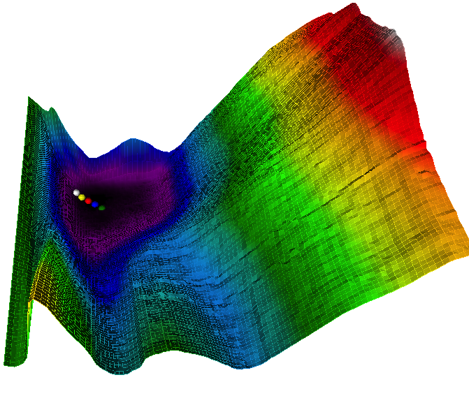
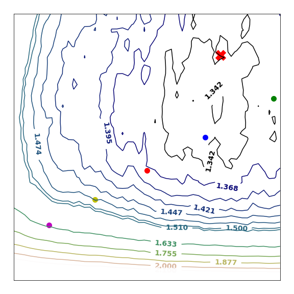
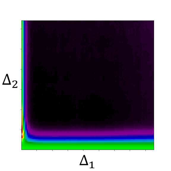
Firstly, it is hard or even impossible to choose an optimal metric for the network performance based on the tensor level quantization error. In particular, even for the same task, similar architectures may favor different objectives. Secondly, the noise in earlier layers might be amplified by successive layers, creating a dependency between quantizaton errors of different layers. This cross-layer dependency makes it necessary to jointly optimize the quantization parameters across all network layers; however, current methods optimize them separately for each layer. Figure 1 plots the challenging loss surface of this optimization process.
Below, we outline the main contributions of the present work along with the organization of the remaining sections.
-
First we consider current layer-by-layer quantization methods where the quantization step size within each layer is optimized to accommodate the dynamic range of the tensor while keeping it small enough to minimize quantization noise. Although these methods optimize the quantization step size of each layer independently of the other layers, we observe strong interactions between the layers, explaining their suboptimal performance at the network level.
-
Accordingly, we consider network quantization as a multivariate optimization problem where the layer quantization step sizes are jointly optimized to minimize the neural network cross-entropy loss. We observe that layer-by-layer quantization identifies solutions in a small region around the optimum, where degradation is quadratic in the distance from it. We provide analytical justification as well as empirical evidence showing this effect.
-
Finally, we propose to combine layer-by-layer quantization with multivariate quadratic optimization. Our method is shown to significantly outperform state-of-the-art methods on two different challenging tasks and six DNN architectures.
2 Related work
The approaches to neural network quantization can be divided roughly into two major categories [15]: quantization-aware training, which introduces the quantization at some point during the training, and post-training quantization, where the network weights are not optimized during the quantization. The recent progress in quantization-aware training has allowed the realization of results comparable to a baseline for as low as 2–4 bits per parameter [2, 25, 9, 24, 12] and show decent performance even for single bit (binary) parameters [17, 22, 13]. The major drawback of quantization-aware methods is the necessity for a vast amount of labeled data and high computational power. Consequently, post-training quantization is widely used in existing embedded hardware solutions. Most work that proposes hardware-friendly post-training schemes has only managed to get to 8-bit quantization without significant degradation in performance or requiring substantial modifications in exisiting hardware.
One of the first post-training schemes, proposed by Gong et al. [8], used min-max ( norm) as a threshold for 8-bit quantization. It produces a small performance degradation and can be deployed efficiently on the hardware. Afterward, better schemes involving the choosing of the clipping value, such as minimizing the Kullback-Leibler divergence [19], assuming the known distribution of weights [1], or minimizing quantization MSE iteratively [14], were proposed.
Another efficient approach quantization is to change the distribution of the tensors, making it more suitable for quantization, such as equalizing the weight ranges [20] or splitting outlier channels [26].
Recent works noted that the quantization process introduces a bias into distributions of the parameters and focused on correction of this bias. Finkelstein et al. [6] addressed a problem of MobileNet quantization. They claimed that the source of degradation was shifting in the mean activation value caused by inherent bias in the quantization process and proposed a scheme for fixing this bias. Multiple alternative schemes for the correction of quantization bias were proposed, and those techniques are widely applied in state-of-the-art quantization approaches [1, 6, 20, 4]. In our work, we utilize the bias correction method by developed Banner et al. [1].
While the simplest form of quantization applies a single quantizer to the whole tensor (weights or activations), finer quantization allows reduction of performance degradation. Even though this approach usually boosts performance significantly [18, 1, 5, 14, 16], it requires more parameters and special hardware support, which makes it unfavorable for real-life deployment.
One more source of performance improvement is using more sophisticated ways to map values to a particular bin. This includes clustering of the tensor entry values [21] and non-uniform quantization [4]. By allowing a more general quantizer, these approaches provide better performance than uniform quantization, but also require hardware support for efficient inference, and thus, similarly to fine-grained quantization, are less suitable for deployment on consumer-grade hardware.
To the best of our knowledge, previous works did not take into account the fact that the loss might be not separable during optimization, usually performed per layer or even per channel. Notable exceptions are Gong et al. [8] and Zhao et al. [26], who did not show any kind of optimization. Nagel et al. [20] partially addressed the lack of separability by treating pairs of consecutive layers together.
3 Loss landscape of quantized DNNs
In this section, we introduce the notion of separability of the loss function. We study the separability and the curvature of the loss function and show how quantization of DNNs affect these properties. Finally, we show that during aggressive quantization, the loss function becomes highly non-separable with steep curvature, which is unfavorable for existing post-training quantization methods. Our method addresses these properties and makes post-training quantization possible at low bit quantization.
We focus on symmetric uniform quantization with a fixed number of bits for all layers and quantization step size that maps a continuous value into a discrete representation,
| (1) |
By constraining the range of to , the connection between and is given by:
| (2) |
In the case of activations, we limit ourselves to the ReLU function, which allows us to choose a quantization range of . In such cases, the quantization step is given by:
| (3) |
3.1 Separable optimization
Suppose the loss function of the network depends on a certain set of variables (weights, activations, etc.), which we denote by a vector . We would like to measure the effect of adding quantization noise to this set of vectors. In the following we show that for sufficiently small quantization noise, we can treat it as an additive noise vector , allowing coordinate-wise optimization. However, when quantization noise is increased, the degradation in one layer is associated with other layers, calling for more laborious non-separable optimization techniques. From the Taylor expansion:
| (4) |
When the quantization error is sufficiently small, higher-order terms can be neglected so that degradation can be approximated as a sum of the quadratic functions,
| (5) |
One can see from Eq. 5 that when quantization error is sufficiently small, the overall degradation can be approximated as a sum of independent separable degradation processes as follows:
| (6) |
On the other hand, when is larger, one needs to take into account the interactions between different layers, corresponding to the second term in Eq. 5 as follows:
| (7) |
where QIT refers to the quantization interaction term.
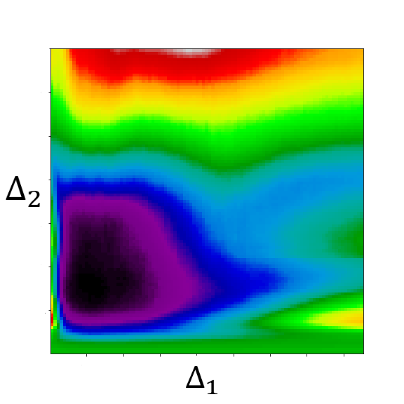
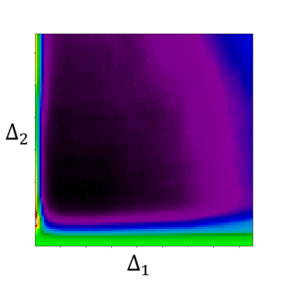
In Fig. 2 we provide a visualization of these interactions at 2, 3 and 4 bitwidth representations.
3.2 Curvature
We now analyze how the steepness of the curvature of the loss function with respect to the quantization step changes as the quantization error increases. We will show that at aggressive quantization, the curvature of the loss becomes steep, which is unfavorable for the methods that aim to minimize quantization error on the tensor level.
We start by defining a measure to quantify curvature of the loss function with respect to quantization step size . Given a quantized neural network, we denote the loss with respect to quantization step size of each individual layer. Since is twice differentiable with respect to we can calculate the Hessian matrix:
| (8) |
To quantify the curvature, we use Gaussian curvature [7], which is given by:
| (9) |
where . We calculated the Gaussian curvature at the point that minimizes the norm of the quantization error and acquired the following values:
| (10) | ||||
| (11) |
This means that the flat surface for 4 bits, shown in Fig. 2, is a generic property of the fine-grained quantization loss and not of the specific layer choice. Similarly, we conclude that coarser quantization generally has steeper curvature than more fine-grained quantization.
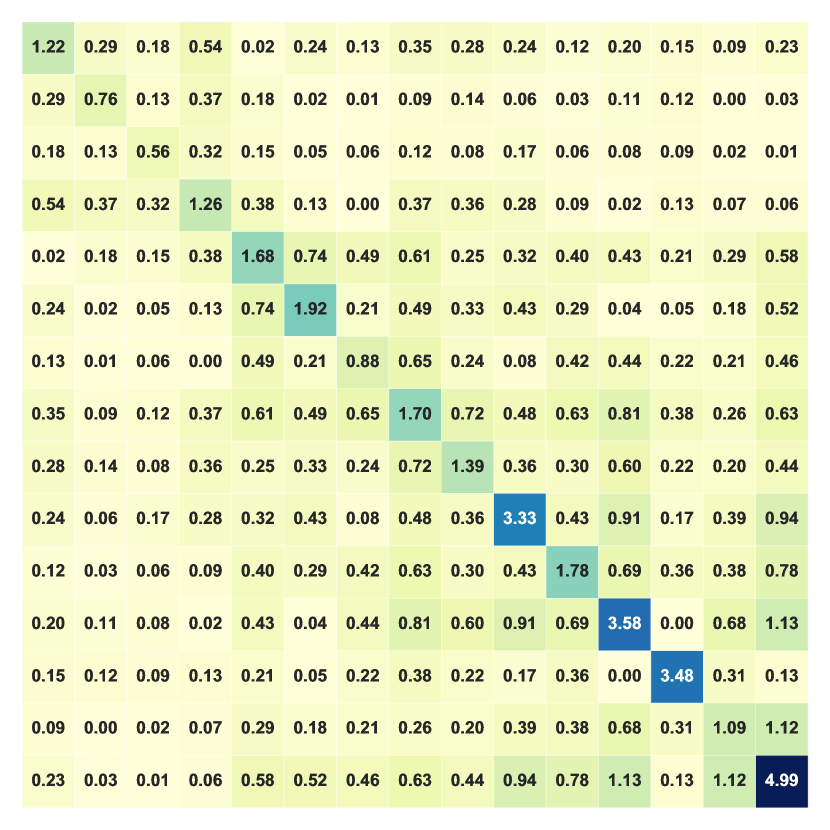
Moreover, the Hessian matrix provides additional information regarding the coupling between different layers. As could be expected, adjacent off-diagonal terms have higher values than distant elements, corresponding to higher dependencies between clipping parameters of adjacent layers (the Hessian matrix is presented in Fig. 0.A.1 in the Appendix).
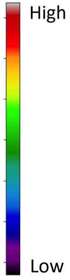
When the curvature is steep, even small changes in quantization step size may change the results drastically. To justify this hypothesis experimentally, in Fig. 3, we evaluate the accuracy of ResNet-50 for five different quantization steps. We choose quantization steps which minimize the norm of the quantization error for different values of .
While at 4-bit quantization, the accuracy is almost not affected by small changes in the quantization step size, at 2-bit quantization, the same changes shift the accuracy by more than 20%. Moreover, the best accuracy is obtained with a quantization step that minimizes and not the MSE, which corresponds to norm minimization.
4 Loss Aware Post-training Quantization (LAPQ)
In the previous section, we showed that the loss function , with respect to the quantization step size , has a complex, non-separable landscape that is hard to optimize. In this section, we suggest a method to overcome this intrinsic difficulty. Our optimization process involves three consecutive steps.
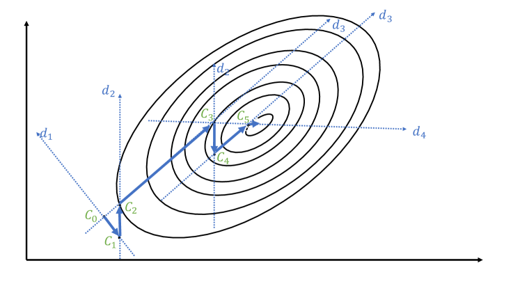
In the first phase, we find the quantization step that minimizes the norm of the quantization error of the individual layers for several different values of . Then, we perform quadratic interpolation to approximate an optimum of the loss with respect to . Finally, we jointly optimize the parameters of all layers acquired on the previous step by applying a gradient-free optimization method [23]. The pseudo-code of the whole algorithm is presented in Algorithm 1. Fig. 6 provides the algorithm visualization.
4.1 Layer-wise optimization
Our method starts by minimizing the norm of the quantization error of weights and activations in each layer with respect to clipping values:
| (12) |
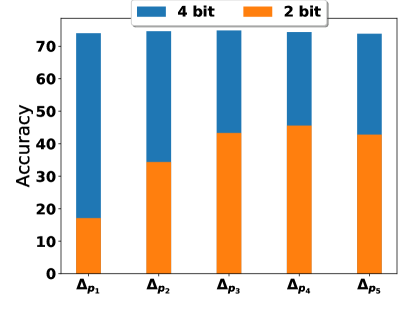
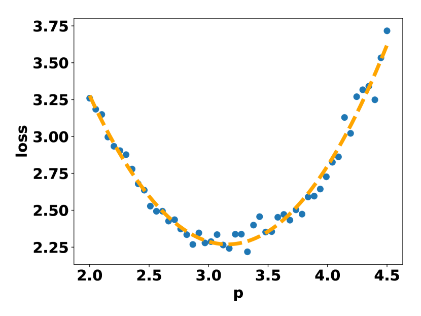
Given a real number , the set of optimal quantization steps , according to Eq. 12, minimizes the quantization error within each layer. In addition, optimizing the quantization error allows us to get in the vicinity of the optimum . Different values of result in different quantization step sizes , which are still optimal under some metric due to the trade-off between clipping and quantization error (Fig. 4).
4.2 Quadratic approximation
Assuming a quantization step size in the vicinity of the optimal quantization step , the loss function can be approximated with a Taylor series as follows:
| (13) | ||||
| (14) |
where is the Hessian matrix with respect to . Since is a minimum, the first derivative vanishes and we acquire a quadratic approximation of ,
| (15) |
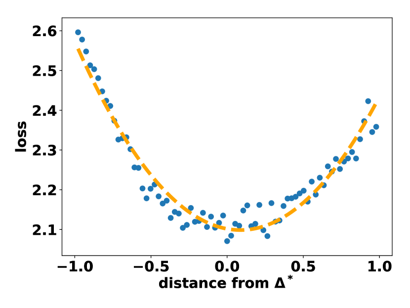
Our method exploits this quadratic property for optimization. Fig. 5(a) demonstrates empirical evidence of such a quadratic relationship for ResNet-18 around the optimal quantization step obtained by our method. First, we sample a few data points to build a trajectory on the graph of (orange points in Fig. 6). Then, we use the prior quadratic assumption to approximate the minimum of the on that trajectory by fitting a quadratic function to the sampled . Finally, we minimize and use the optimal quantization step size as a starting point for a gradient-free joint optimization algorithm, such as Powell’s method [23], to minimize the loss and find .
4.3 Joint optimization
By minimizing both the quantization error and the loss using quadratic interpolation, we get a decent approximation of the global minimum . Due to steep curvature of the minimum, however, for a low bitwidth quantization, even a small error in the value of leads to performance degradation. Thus, we use a gradient-free joint optimization, specifically an iterative algorithm (Powell’s method [23]), to further optimize .
At every iteration, we optimize the set of parameters, initialized by . Given a set of linear search directions , the new position is expressed by the linear combination of the search directions as following . The new displacement vector becomes part of the search directions set, and the search vector, which contributed most to the new direction, is deleted from the search directions set. For further details, see Algorithm 1.
5 Experimental Results
In this section we conduct extensive evaluations and offer a comparison to prior art of the proposed method on two challenging benchmarks, image classification on ImageNet and a recommendation system on NCF-1B. In addition, we examine the impact of each part of the proposed method on the final accuracy. In all experiments we first calibrate the optimal clipping values on a small held-back calibration set using our method and then evaluate the validation set.
5.1 ImageNet
| Model | W/A | Method | Accuracy(%) |
| 32 / 32 | FP32 | 69.7 | |
| LAPQ (Ours) | 68.8 | ||
| DUAL [14] | 68.38 | ||
| ACIQ [1] | 65.528 | ||
| 8 / 4 | MMSE | 68 | |
| LAPQ (Ours) | 66.3 | ||
| ACIQ [1] | 52.476 | ||
| 8 / 3 | MMSE | 63.3 | |
| LAPQ (Ours) | 60.3 | ||
| ACIQ [1] | 4.1 | ||
| KLD [19] | 31.937 | ||
| ResNet-18 | 4 / 4 | MMSE | 43.6 |
| 32 / 32 | FP32 | 76.1 | |
| LAPQ (Ours) | 74.8 | ||
| DUAL [14] | 73.25 | ||
| ACIQ [1] | 68.92 | ||
| 8 / 4 | MMSE | 74 | |
| LAPQ (Ours) | 70.8 | ||
| ACIQ [1] | 51.858 | ||
| 8 / 3 | MMSE | 66.3 | |
| LAPQ (Ours) | 70 | ||
| ACIQ [1] | 3.3 | ||
| KLD [19] | 46.19 | ||
| ResNet-50 | 4 / 4 | MMSE | 36.4 |
| Model | W/A | Method | Accuracy(%) |
| 32 / 32 | FP32 | 77.3 | |
| LAPQ (Ours) | 73.6 | ||
| DUAL [14] | 74.26 | ||
| ACIQ [1] | 66.966 | ||
| 8 / 4 | MMSE | 72 | |
| LAPQ (Ours) | 65.7 | ||
| ACIQ [1] | 41.46 | ||
| 8 / 3 | MMSE | 56.7 | |
| LAPQ (Ours) | 59.2 | ||
| ACIQ [1] | 1.5 | ||
| KLD [19] | 49.948 | ||
| ResNet-101 | 4 / 4 | MMSE | 9.8 |
| 32 / 32 | FP32 | 77.2 | |
| LAPQ (Ours) | 75.1 | ||
| DUAL [14] | 73.06 | ||
| ACIQ [1] | 66.42 | ||
| 8 / 4 | MMSE | 74.3 | |
| LAPQ (Ours) | 64.4 | ||
| ACIQ [1] | 31.01 | ||
| 8 / 3 | MMSE | 54.1 | |
| LAPQ (Ours) | 38.6 | ||
| ACIQ [1] | 0.5 | ||
| KLD [19] | 1.84 | ||
| Inception-V3 | 4 / 4 | MMSE | 2.2 |
We evaluate our method on several CNN architectures on ImageNet. We select a calibration set of 512 random images for the optimization step. The size of the calibration set defines the trade-off between generalization and running time (the analysis is given in Appendix 0.B). Following the convention [2, 24], we do not quantize the first and last layers.
Many successful methods of post-training quantization perform finer parameter assignment, such as group-wise [18], channel-wise [1], pixel-wise [5] or filter-wise [14] quantization, which require special hardware support and additional computational resources. Finer parameter assignment appears to provide unconditional improvement, independently of the underlying methods used. In contrast with those approaches, our method performs layer-wise quantization, which is simple to implement on any existing hardware that supports low precision integer operations. Thus, we do not include the above-mentioned methods in our comparison study. We apply bias correction, as proposed by Banner et al. [1], on top of the proposed method. In Table 1 (more results are available in Table 0.C.1 in the Appendix) we compare our method with several other layer-wise quantization methods, as well as the minimal MSE baseline. In most cases, our method significantly outperforms all the competing methods, showing acceptable performance even for 4-bit quantization.
5.2 NCF-1B
In addition to the vision models, we evaluated our method on a recommendation system task, specifically on a Neural Collaborative Filtering (NCF) [10] model. We use mlperf111https://github.com/mlperf/training/tree/master/recommendation/pytorch implementation to train the model on the MovieLens-1B dataset. Similarly to the ImageNet, the calibration set of 50k random user/item pairs is significantly smaller than both the training and validation sets.
| Model | W/A | Method | Hit rate(%) |
|---|---|---|---|
| NCF 1B | 32/32 | FP32 | 51.5 |
| 32/8 | LAPQ (Ours) | 51.2 | |
| MMSE | 51.1 | ||
| 8/32 | LAPQ (Ours) | 51.4 | |
| MMSE | 33.4 | ||
| 8/8 | LAPQ (Ours) | 51.0 | |
| MMSE | 33.5 |
In Table 2 we present results for the NCF-1B model compared to the MMSE method. Even at 8-bit quantization, NCF-1B suffers from significant degradation when using the naive MMSE method. In contrast, LAPQ achieves near baseline accuracy with 0.5% degradation from FP32 results.
5.3 Ablation study
Initialization
The proposed method comprises of two steps: layer-wise optimization and quadratic approximation as the initialization for the joint optimization. In Table 3, we show the results for ResNet-18 under different initializations and their results after adding the joint optimization. LAPQ suggest a better initialization for the joint optimization.
| W / A | Method | Accuracy (%) | |
|---|---|---|---|
| Initial | Joint | ||
| 4 / 4 | Random | 0.1 | 7.8 |
| LW | 43.6 | 57.8 | |
| LW + QA | 54.1 | 60.3 | |
| 32 / 2 | Random | 0.1 | 0.1 |
| LW | 33 | 50.3 | |
| LW + QA | 48.1 | 50.7 | |
Bias correction
Prior research [1, 6] has shown that CNNs are sensitive to quantization bias. To address this issue, we perform bias correction of the weights as proposed by Banner et al. [1], which can easily be combined with LAPQ, in all our CNN experiments. In Table 4 we show the effect of adding bias correction to the proposed method and compare it with MMSE. We see that bias correction is especially important in compact models, such as MobileNet.
| W | A | ResNet-18 | ResNet-50 | MobileNet-V2 |
|---|---|---|---|---|
| LAPQ | ||||
| 32 | 4 | 68.8% | 74.8% | 65.1% |
| 32 | 2 | 51.6% | 54.2% | 1.5% |
| 4 | 32 | 62.6% | 69.9% | 29.4% |
| 4 | 4 | 58.5% | 66.6% | 21.3% |
| LAPQ + bias correction | ||||
| 4 | 32 | 63.3% | 71.8% | 60.2% |
| 4 | 4 | 59.8% | 70.% | 49.7% |
| FP32 | 69.7% | 76.1% | 71.8% | |
6 Conclusion
We have analyzed the loss function of quantized neural networks. At low precision, the function is non-separable, with steep curvature, which is unfavorable for existing post-training quantization methods. Accordingly, we have introduced Loss Aware Post-training Quantization (LAPQ), which jointly optimizes all quantization parameters by minimizing the loss function directly. We have shown that our method outperforms current post-training quantization methods. Also, our method does not require special hardware support such as channel-wise or filter-wise quantization. In some models, LAPQ is the first to show compatible performance in 4-bit post-training quantization regime with layer-wise quantization, almost achieving a the full-precision baseline accuracy.
Acknowledgments
The research was funded by National Cyber Security Authority and the Hiroshi Fujiwara Technion Cyber Security Research Center.
References
- Banner et al. [2018] Banner, R., Nahshan, Y., Hoffer, E., Soudry, D.: Post-training 4-bit quantization of convolution networks for rapid-deployment. arXiv preprint arXiv:1810.05723 (2018), URL http://arxiv.org/abs/1810.05723
- Baskin et al. [2018] Baskin, C., Liss, N., Chai, Y., Zheltonozhskii, E., Schwartz, E., Girayes, R., Mendelson, A., Bronstein, A.M.: Nice: Noise injection and clamping estimation for neural network quantization. arXiv preprint arXiv:1810.00162 (2018), URL http://arxiv.org/abs/1810.00162
- Bethge et al. [2019] Bethge, J., Yang, H., Bornstein, M., Meinel, C.: Back to simplicity: How to train accurate bnns from scratch? arXiv preprint arXiv:1906.08637 (2019), URL http://arxiv.org/abs/1906.08637
- Fang et al. [2020] Fang, J., Shafiee, A., Abdel-Aziz, H., Thorsley, D., Georgiadis, G., Hassoun, J.: Near-lossless post-training quantization of deep neural networks via a piecewise linear approximation. arXiv preprint arXiv:2002.00104 (2020), URL https://arxiv.org/abs/2002.00104
- Faraone et al. [2018] Faraone, J., Fraser, N., Blott, M., Leong, P.H.: Syq: Learning symmetric quantization for efficient deep neural networks. In: The IEEE Conference on Computer Vision and Pattern Recognition (CVPR) (June 2018), URL http://openaccess.thecvf.com/content_cvpr_2018/html/Faraone_SYQ_Learning_Symmetric_CVPR_2018_paper.html
- Finkelstein et al. [2019] Finkelstein, A., Almog, U., Grobman, M.: Fighting quantization bias with bias. arXiv preprint arXiv:1906.03193 (2019), URL http://arxiv.org/abs/1906.03193
- Goldman [2005] Goldman, R.: Curvature formulas for implicit curves and surfaces. Computer Aided Geometric Design 22(7), 632 – 658 (2005), ISSN 0167-8396, doi:https://doi.org/10.1016/j.cagd.2005.06.005, URL http://www.sciencedirect.com/science/article/pii/S0167839605000737, geometric Modelling and Differential Geometry
- Gong et al. [2018] Gong, J., Shen, H., Zhang, G., Liu, X., Li, S., Jin, G., Maheshwari, N., Fomenko, E., Segal, E.: Highly efficient 8-bit low precision inference of convolutional neural networks with intelcaffe. In: Proceedings of the 1st on Reproducible Quality-Efficient Systems Tournament on Co-designing Pareto-efficient Deep Learning, ReQuEST ’18, ACM, New York, NY, USA (2018), ISBN 978-1-4503-5923-8, doi:10.1145/3229762.3229763, URL http://doi.acm.org/10.1145/3229762.3229763
- Gong et al. [2019] Gong, R., Liu, X., Jiang, S., Li, T., Hu, P., Lin, J., Yu, F., Yan, J.: Differentiable soft quantization: Bridging full-precision and low-bit neural networks. In: The IEEE International Conference on Computer Vision (ICCV) (October 2019), URL http://openaccess.thecvf.com/content_ICCV_2019/html/Gong_Differentiable_Soft_Quantization_Bridging_Full-Precision_and_Low-Bit_Neural_Networks_ICCV_2019_paper.html
- He et al. [2017] He, X., Liao, L., Zhang, H., Nie, L., Hu, X., Chua, T.S.: Neural collaborative filtering. In: Proceedings of the 26th International Conference on World Wide Web, pp. 173–182, WWW ’17, International World Wide Web Conferences Steering Committee, Republic and Canton of Geneva, Switzerland (2017), ISBN 978-1-4503-4913-0, doi:10.1145/3038912.3052569, URL https://doi.org/10.1145/3038912.3052569
- Hubara et al. [2017] Hubara, I., Courbariaux, M., Soudry, D., El-Yaniv, R., Bengio, Y.: Quantized neural networks: Training neural networks with low precision weights and activations. J. Mach. Learn. Res. 18(1), 6869–6898 (Jan 2017), ISSN 1532-4435, URL http://dl.acm.org/citation.cfm?id=3122009.3242044
- Jin et al. [2019] Jin, Q., Yang, L., Liao, Z.: Towards efficient training for neural network quantization. arXiv preprint arXiv:1912.10207 (2019), URL https://arxiv.org/abs/1912.10207
- Kim et al. [2020] Kim, H., Kim, K., Kim, J., Kim, J.J.: Binaryduo: Reducing gradient mismatch in binary activation network by coupling binary activations. arXiv preprint arXiv:2002.06517 (2020), URL https://arxiv.org/abs/2002.06517
- Kravchik et al. [2019] Kravchik, E., Yang, F., Kisilev, P., Choukroun, Y.: Low-bit quantization of neural networks for efficient inference. In: The IEEE International Conference on Computer Vision (ICCV) Workshops (Oct 2019), URL http://openaccess.thecvf.com/content_ICCVW_2019/html/CEFRL/Kravchik_Low-bit_Quantization_of_Neural_Networks_for_Efficient_Inference_ICCVW_2019_paper.html
- Krishnamoorthi [2018] Krishnamoorthi, R.: Quantizing deep convolutional networks for efficient inference: A whitepaper. arXiv preprint arXiv:1806.08342 (2018), URL http://arxiv.org/abs/1806.08342
- Lee et al. [2018] Lee, J.H., Ha, S., Choi, S., Lee, W.J., Lee, S.: Quantization for rapid deployment of deep neural networks. arXiv preprint arXiv:1810.05488 (2018), URL http://arxiv.org/abs/1810.05488
- Liu et al. [2019] Liu, C., Ding, W., Xia, X., Hu, Y., Zhang, B., Liu, J., Zhuang, B., Guo, G.: Rectified binary convolutional networks for enhancing the performance of 1-bit DCNNs. In: Proceedings of the Twenty-Eighth International Joint Conference on Artificial Intelligence, IJCAI-19, pp. 854–860, International Joint Conferences on Artificial Intelligence Organization (7 2019), doi:10.24963/ijcai.2019/120, URL https://doi.org/10.24963/ijcai.2019/120
- Mellempudi et al. [2017] Mellempudi, N., Kundu, A., Mudigere, D., Das, D., Kaul, B., Dubey, P.: Ternary neural networks with fine-grained quantization. arXiv preprint arXiv:1705.01462 (2017), URL http://arxiv.org/abs/1705.01462
- Migacz [2017] Migacz, S.: 8-bit inference with tensorrt (2017), URL http://on-demand.gputechconf.com/gtc/2017/presentation/s7310-8-bit-inference-with-tensorrt.pdf
- Nagel et al. [2019] Nagel, M., Baalen, M.v., Blankevoort, T., Welling, M.: Data-free quantization through weight equalization and bias correction. In: Proceedings of the IEEE International Conference on Computer Vision, pp. 1325–1334 (2019), URL http://openaccess.thecvf.com/content_ICCV_2019/html/Nagel_Data-Free_Quantization_Through_Weight_Equalization_and_Bias_Correction_ICCV_2019_paper.html
- Nayak et al. [2019] Nayak, P., Zhang, D., Chai, S.: Bit efficient quantization for deep neural networks. arXiv preprint arXiv:1910.04877 (2019), URL http://arxiv.org/abs/1910.04877
- Peng and Chen [2019] Peng, H., Chen, S.: Bdnn: Binary convolution neural networks for fast object detection. Pattern Recognition Letters (2019), ISSN 0167-8655, doi:https://doi.org/10.1016/j.patrec.2019.03.026, URL http://www.sciencedirect.com/science/article/pii/S0167865519301096
- Powell [1964] Powell, M.J.: An efficient method for finding the minimum of a function of several variables without calculating derivatives. The Computer Journal 7(2), 155 (1964), doi:10.1093/comjnl/7.2.155, URL http://dx.doi.org/10.1093/comjnl/7.2.155
- Yang et al. [2019] Yang, J., Shen, X., Xing, J., Tian, X., Li, H., Deng, B., Huang, J., Hua, X.s.: Quantization networks. In: The IEEE Conference on Computer Vision and Pattern Recognition (CVPR) (June 2019), URL http://openaccess.thecvf.com/content_CVPR_2019/html/Yang_Quantization_Networks_CVPR_2019_paper.html
- Zhang et al. [2018] Zhang, D., Yang, J., Ye, D., Hua, G.: Lq-nets: Learned quantization for highly accurate and compact deep neural networks. In: The European Conference on Computer Vision (ECCV) (September 2018), URL http://openaccess.thecvf.com/content_ECCV_2018/html/Dongqing_Zhang_Optimized_Quantization_for_ECCV_2018_paper.html
- Zhao et al. [2019] Zhao, R., Hu, Y., Dotzel, J., De Sa, C., Zhang, Z.: Improving neural network quantization using outlier channel splitting. arXiv preprint arXiv:1901.09504 (2019), URL https://arxiv.org/abs/1901.09504
Appendix 0.A Hessian of the loss function
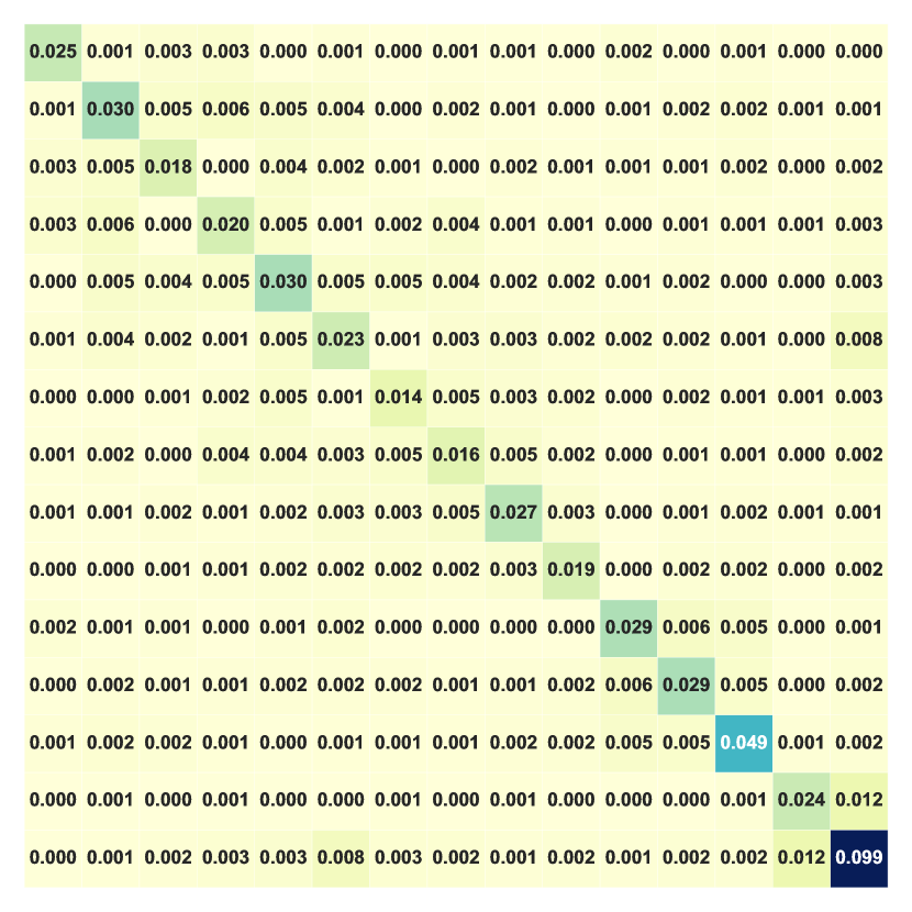
To estimate dependencies between clipping parameters of different layers, we analyze the structure of the Hessian matrix of the loss function. The Hessian matrix contains the second-order partial derivatives of the loss , where is a vector of quantization steps:
| (0.A.16) |
In the case of separable functions, the Hessian is a diagonal matrix. This means that the magnitude of the off-diagonal elements can be used as a measure of separability. In Fig. 0.A.1 we show the Hessian matrix of the loss function under quantization of 4 and 2 bits. As expected, higher dependencies between quantization steps emerge under more aggressive quantization.
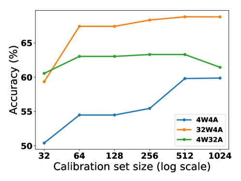
Appendix 0.B Calibration set size
Calibration set size reflects the balance between the running time and the generalization. To determine the required size, we ran the proposed method on ResNet-18 for various calibration set sizes and different bitwidths. As shown in Fig. 0.B.2, a calibration set size of 512 is a good choice to balance this trade-off.
Appendix 0.C ImageNet additional results
In Table 0.C.1 we show additional results for the proposed method for the image classification task on ImageNet dataset.
| Model | W/A | Method | Accuracy(%) |
|---|---|---|---|
| 32 / 32 | FP32 | 69.7 | |
| ResNet-18 | 8 / 2 | LAPQ (Ours) | 51.6 |
| ACIQ [1] | 7.07 | ||
| 32 / 32 | FP32 | 76.1 | |
| LAPQ (Ours) | 54.2 | ||
| 8 / 2 | ACIQ [1] | 2.92 | |
| LAPQ (Ours) | 71.8 | ||
| ResNet-50 | 4 / 32 | OCS [26] | 69.3 |
| 32 / 32 | FP32 | 77.3 | |
| LAPQ (Ours) | 29.8 | ||
| 8 / 2 | ACIQ [1] | 3.826 | |
| LAPQ (Ours) | 66.5 | ||
| ResNet-101 | 4 / 32 | MMSE | 18 |