On entanglement hamiltonians of an interval
in massless harmonic chains
Abstract
We study the continuum limit of the entanglement hamiltonians of a block of consecutive sites in massless harmonic chains. This block is either in the chain on the infinite line or at the beginning of a chain on the semi-infinite line with Dirichlet boundary conditions imposed at its origin. The entanglement hamiltonians of the interval predicted by Conformal Field Theory for the massless scalar field are obtained in the continuum limit. We also study the corresponding entanglement spectra and the numerical results for the ratios of the gaps are compatible with the operator content of the Boundary Conformal Field Theory of a massless scalar field with Neumann boundary conditions imposed along the boundaries introduced around the entangling points by the regularisation procedure.
Contents
toc
1 Introduction
Entanglement has attracted an intense research activity during the last two decades, mostly focused on theoretical approaches [1, 2, 3, 4], but in the last few years also experimental setups have been realised to detect its characteristic features [5].
Given a quantum system in a state described by the density matrix , assuming that its Hilbert space can be factorised as , the reduced density matrix is defined by tracing out the degrees of freedom of , namely by , with the normalisation condition . The reduced density matrix can be written as , where the hermitian operator is the entanglement hamiltonian (also known as modular hamiltonian) and . The entanglement entropy is easily obtained from the eigenvalues of [6, 7, 8]. Important results have been obtained for factorisations of the Hilbert space corresponding to bipartitions of the space, namely when is a spatial region and its complement. In these cases the hypersurface separating and is called entangling hypersurface.
A fundamental theorem proved by Bisognano and Wichmann [9] in the context of Algebraic Quantum Field Theory claims that, given a relativistic Quantum Field Theory (QFT) in dimensions in its vacuum state (we denote by the dimensional position vector) and the spatial bipartition where corresponds to half space and the entangling hypersurface is the flat hyperplane, the entanglement hamiltonian of can be written as an integral over the half space of the energy density of the QFT as follows
| (1) |
When the QFT is a Conformal Field Theory (CFT), the conformal symmetry allows to write analytic expressions for the entanglement hamiltonians for simple spatial bipartitions, mainly at equilibrium [10, 11, 12, 13, 14] but in few cases also out of equilibrium [13]. More complicated bipartitions require a detailed knowledge of the underlying CFT [15, 16].
In a dimensional CFT at equilibrium in its vacuum state, we consider bipartitions where is an interval and such that its entanglement hamiltonian can be written as
| (2) |
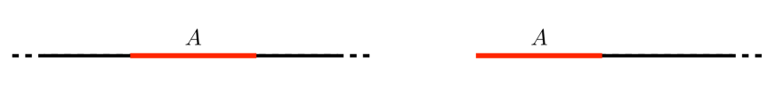
where is the length of and depends on the bipartition. In this manuscript we focus on the bipartitions shown in Fig. 1. For an interval in the infinite line (left panel in Fig. 1), the weight function in (2) is the following parabola [10, 11]
| (3) |
When is an interval at the beginning of a semi-infinite line (right panel in Fig. 1), the weight function in (2) is the half parabola given by [13]
| (4) |
independently of the boundary conditions imposed at the beginning of the semi-infinite line. It is interesting to explore the procedure that allows to obtain these entanglement hamiltonians in CFT as the continuum limit of the corresponding entanglement hamiltonians in the lattice models providing a discretisation of the CFT.
Entanglement hamiltonians in free lattice models at equilibrium in their ground state have been studied in [1, 2, 17, 18, 20, 21, 19, 22]. A detailed analysis of the continuum limit has been recently carried out for an interval in an infinite chain of free fermions [22], by employing the analytic results obtained by Eisler and Peschel in [20]. In this manuscript we study the continuum limit of the entanglement hamiltonians of a block of consecutive sites in massless harmonic chains by following the approach of [22], which is based on the observation that, in this limit, the proper combinations of all the diagonals of the matrices determining the entanglement hamiltonian on the lattice must be considered [19].
The eigenvalues of the entanglement hamiltonian provide the entanglement spectrum, which contains relevant physical information [23]. It is worth introducing the gaps with respect to the largest eigenvalue and also their ratios with respect to the smallest gap . We remark that these ratios are not influenced by a global shift and a rescaling of the entire spectrum.
In a two dimensional QFT in imaginary time, a useful way to regularise the ultraviolet (UV) divergences consists in removing infinitesimal disks whose radius is the UV cutoff around the entangling points of the bipartition [7, 18, 24, 13]. In two dimensional CFT, this regularisation procedure leads to a Boundary Conformal Field Theory (BCFT) [25] if proper conformal boundary conditions are imposed along the boundaries in the euclidean spacetime (both the boundaries given by the physical boundaries of the system and the ones due to this regularisation procedure must be considered). For a class of entanglement hamiltonians which includes the ones we are interested in, it has been found that [13]
| (5) |
where and are the non vanishing elements of the conformal spectrum (made by conformal dimensions of the primary fields and of their descendants) of the underlying BCFT. Numerical evidences that the conformal spectrum of a BCFT provides the entanglement spectrum have been first obtained at equilibrium by Läuchli in [26] and more recently also out of equilibrium [27, 28].
In this manuscript we focus on massless harmonic chains and perform a numerical analysis of the continuum limit of two entanglement hamiltonians of an interval and of the corresponding entanglement spectra. We consider a massless harmonic chain both on the infinite line and on the semi-infinite line with Dirichlet boundary conditions imposed at its origin. The continuum limit of these lattice models is the CFT given by the massless scalar field , whose central charge is . By introducing the canonical momentum field , the energy density on the infinite line reads
| (6) |
and on the semi-infinite line is given by [29]
| (7) |
We study the spatial bipartitions shown in Fig. 1, whose entanglement hamiltonians predicted by CFT are given by (2), (3) and (6) for the interval in the infinite line and by (2), (4) and (7) for the interval at the beginning of the semi-infinite line. Our numerical analysis is based on the procedure described in [20, 22] to study the continuum limit of the entanglement hamiltonian of an interval in an infinite chain of free fermions. We study also the entanglement spectra of these entanglement hamiltonians, finding that the CFT prediction (5) holds, once Neumann boundary conditions are imposed along the boundaries introduced by the regularisation procedure.
This manuscript is organised as follows. In §2 we report the entanglement hamiltonian of an interval in harmonic chains in terms of the two-point correlators. In §3 we study the continuum limit of the entanglement hamiltonian of an interval in the infinite line and in §4 this analysis is performed for an interval at the beginning of the semi-infinite line with Dirichlet boundary conditions. In §5 we draw some conclusions. The Appendix A contains further results supporting some observations made in the main text.
2 Entanglement hamiltonians in the harmonic chain
In this section we report the expression of the entanglement hamiltonian of a subsystem in harmonic chains in terms of the two-point correlators [2], discussing also some decompositions that will be employed throughout the manuscript.
The hamiltonian of the harmonic chain with nearest neighbour spring-like interaction reads
| (8) |
where the position and the momentum operators and are hermitean operators satisfying the canonical commutation relations and ( throughout this manuscript). In our numerical analysis we set .
The hamiltonian (8) is the discretization of the hamiltonian of a massive scalar field in the continuum, whose massless regime given by is a CFT with central charge . The range of the index in (8) depends on the spatial domain supporting the harmonic chain: in this manuscript we consider either the infinite line () or the semi-infinite line (integer ). When (8) is defined on the semi-infinite line, it is crucial to specify also the boundary condition imposed at the beginning of the semi-infinite line (i.e. at ) and in our analysis we consider the case of Dirichlet boundary conditions. The two-point correlators and provide the generic elements of the correlation matrices and respectively.
Let us consider harmonic chains (8) in their ground state and introduce the bipartition of the chain into a spatial domain made by sites and its complement , assuming that the Hilbert space can be bipartite accordingly as . Since for these quantum systems the reduced density matrix remains Gaussian, independently of the choice of the bipartition, the corresponding entanglement hamiltonian is a quadratic hermitian operator, which can be written as follows [17, 2]
| (9) |
where the dimensional vector collects the position and the momentum operators and with . The matrix is real, symmetric and positive definite; hence is hermitian. In terms of the reduced correlation matrices and , obtained by restricting and to the subsystem , the matrix can be evaluated as follows [2]
where
| (11) |
The equivalence of the two expressions in (2) can be verified by transposing one of them and employing that and are symmetric (we also need , which is easily obtained from the fact that and are symmetric).
In this manuscript we study entanglement hamiltonians when the entire chain is at equilibrium in its ground state and when the subsystem is a block of consecutive sites either in the infinite line or at the beginning of the semi-infinite line where Dirichlet boundary conditions are imposed (see Fig. 1). In these two cases, the matrix is block diagonal. The off-diagonal blocks of can be non vanishing e.g. for the time dependent entanglement hamiltonians after a global quantum quench [27].
The matrix can be constructed numerically through (2) and (11). In order to employ these formulas, the eigenvalues of the matrix must be strictly larger than . In our numerical analysis many eigenvalues very close to occur and the software automatically approximates them to whenever a low numerical precision is set throughout the numerical analysis. This forces us to work with very high numerical precisions. In particular we have employed precisions up to 6500 digits, depending on the specific calculation. We observe that higher precision is required as and increase.
The expressions (9) and (2) naturally lead to write the entanglement hamiltonian in terms of the symmetric matrices and as follows
| (12) |
where
| (13) |
These sums can be organised in different ways. For instance, by writing the symmetric matrices and as sums of a diagonal matrix, an upper triangular matrix and a lower triangular matrix, it is straightforward to obtain
| (14) | |||||
| (15) |
In [19] the sums (13) have been rewritten by decomposing the contribution coming from the -th row of the matrices and , and this leads to
| (16) | |||||
| (17) |
We find it convenient to introduce also the following decomposition
| (18) | |||
where the contribution of the counter diagonal has been included into the summation over . This choice leads to an inconsistency in the range of of the last double sum when , which can be easily fixed by imposing the vanishing of this term.
An alternative decomposition, inspired by the numerical analysis performed in [22], is discussed in Appendix A. In our numerical analysis we have tested all the decompositions introduced above and in Appendix A for both the spatial bipartitions shown in Fig. 1. In the main text we show the numerical results obtained from (2) and (2), while the results found through the other decompositions have been reported in Appendix A.
The analytic results for the entanglement hamiltonian of an interval in the infinite chain of free fermions found in [20, 22] and the decompositions introduced above for the operators and suggest to introduce the following limits
| (20) |
where is the midpoint between the -th and the -th site. The existence of the functions and is a crucial assumption in the subsequent derivations of the CFT predictions for the entanglement hamiltonians.
3 Interval in the infinite line
In this section we consider the harmonic chain on the infinite line and perform a numerical analysis to study the continuum limit of the entanglement hamiltonian of an interval. We follow the procedure discussed in [20, 22] for the continuum limit of the entanglement hamiltonian of an interval in the infinite chain of free fermions. In §3.1 we introduce the two-point correlators to construct and and in §3.2 we report the main analysis, which leads to the CFT prediction (2), with the weight function (3) and the energy density (6). The entanglement spectrum is explored in §3.3.
3.1 Correlators
The two-point correlators and in the ground state of a finite harmonic chain made by sites ( in (8)) with periodic boundary conditions ( and ) are respectively
| (21) |
where the dispersion relation reads
| (22) |
The translation invariance induces the occurrence of the zero mode, that corresponds to . Since , it is straightforward to observe that diverges as ; hence the mass cannot be set to zero in the numerical analysis of this system.
In the thermodynamic limit , the correlators in (21) can be written as the integrals
| (23) | |||||
| (24) |
which can be evaluated analytically, finding the following expressions in terms of the hypergeometric function [30]
| (25) | |||||
| (26) |
where the parameter is defined as
| (27) |
The reduced correlation matrices and are obtained by restricting the indices and of the correlators (25) and (26) to the interval , i.e. to the integer values in . By employing these reduced correlation matrices into (2), one finds the entanglement hamiltonian matrix . The entanglement hamiltonian of the interval in the infinite line is obtained by plugging the matrix into (9).
3.2 Entanglement hamiltonian
The entanglement hamiltonian of a block made by consecutive sites in the infinite line, when the entire harmonic chain is in its ground state, is the operator constructed as explained in §3.1. Considering the massless regime, we study the procedure to obtain the CFT prediction (2), with and given by (3) and (6) respectively, through a numerical analysis of the continuum limit.
The translation invariance of the entire system prevents us from setting in our numerical analysis, as already remarked in §3.1. The data reported in all the figures discussed in this subsection have been obtained for . The choice of this value is discussed in Appendix A.
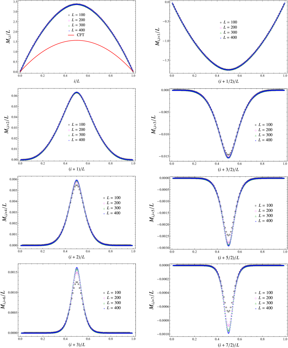
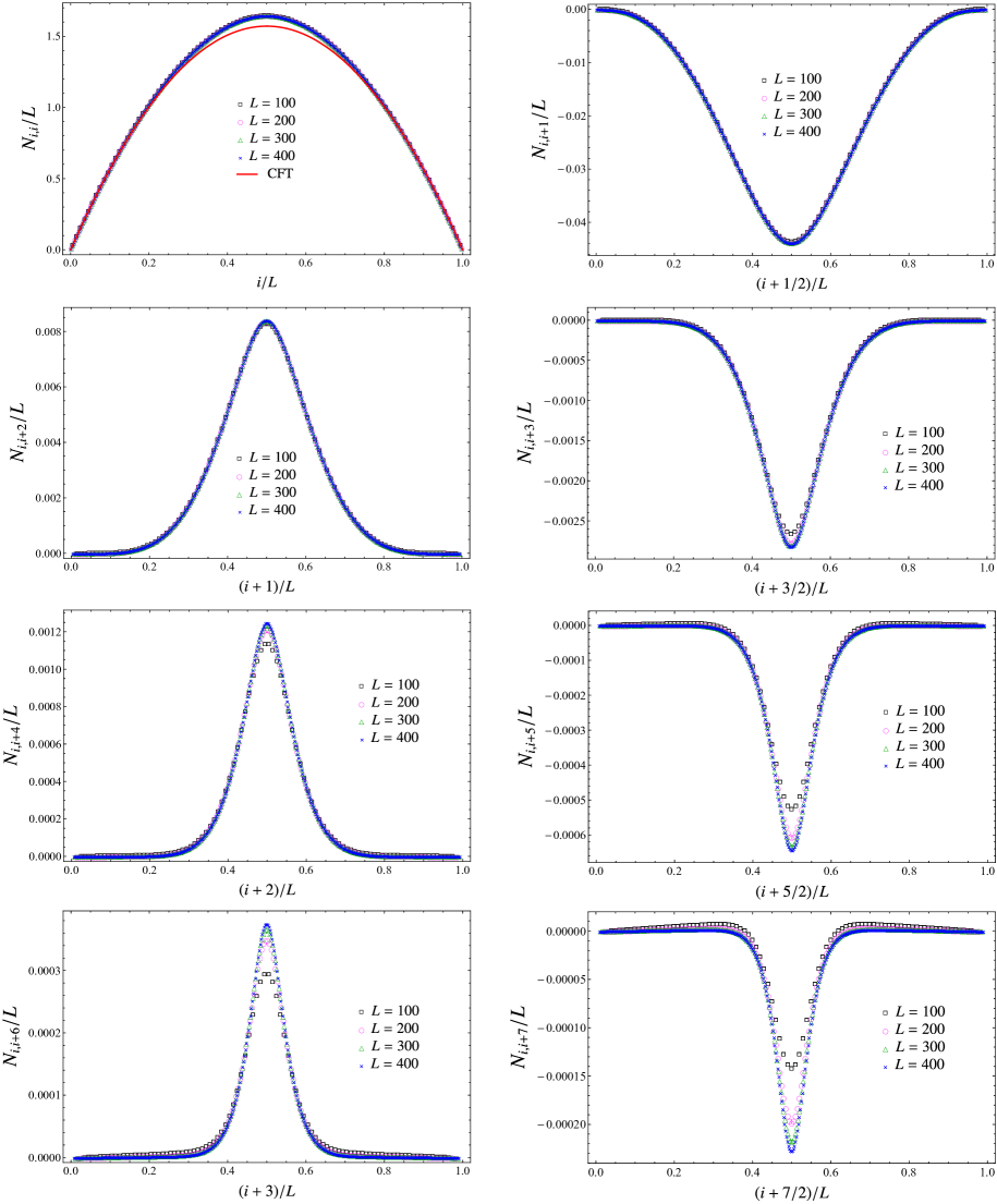
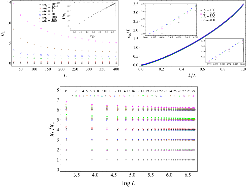
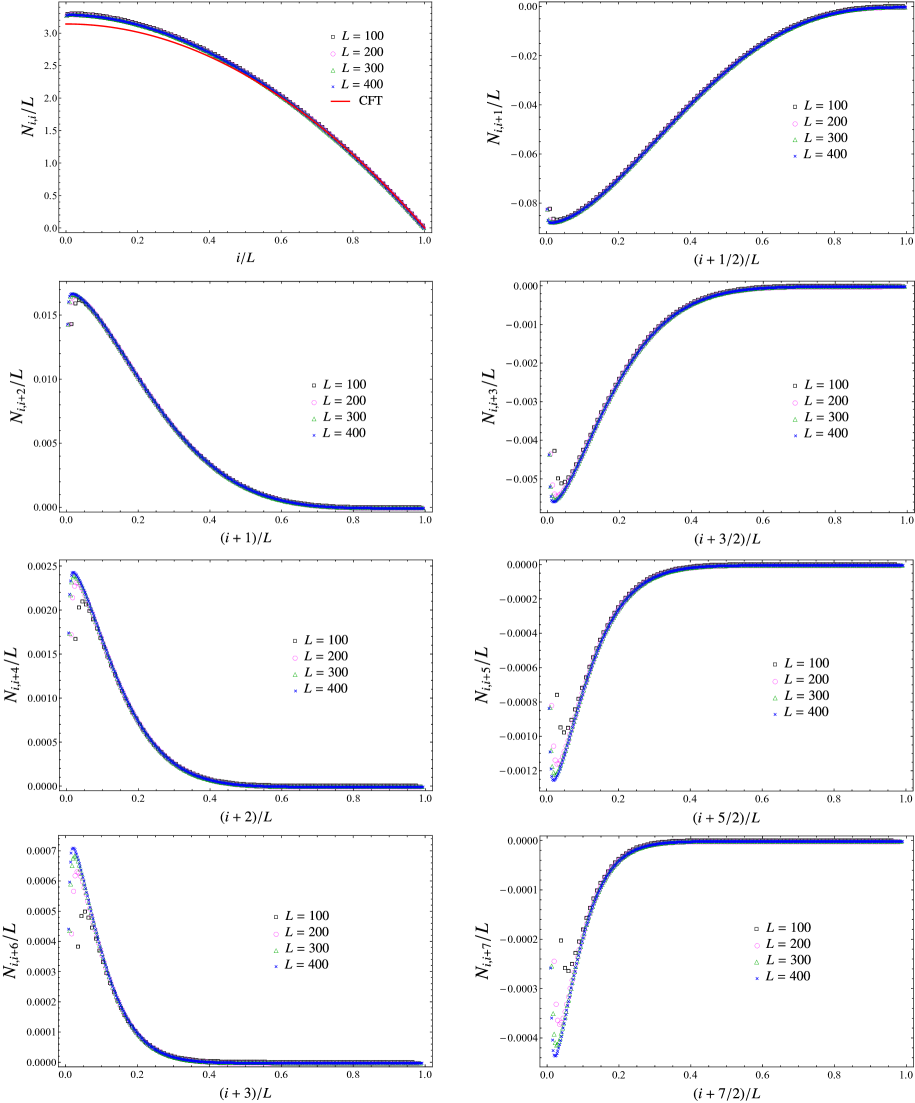
In Fig. 2 and Fig. 3 we show the data for the diagonals and with for some values of . This numerical results lead to conclude that the limits in (20) provide well defined functions. Furthermore, these functions have a well defined sign given by the parity of , are symmetric under reflection with respect to the center of the interval (we checked numerically that this symmetry holds also for the data points, i.e. that and ) and the absolute value of their maximum significantly decreases as increases. It would be interesting to find analytic expressions for the functions defined through the limits (20), as done in [20] for the interval in the infinite chain of free fermions.
Assuming that the functions and introduced in (20) are well defined, let us study the continuum limit of the entanglement hamiltonian (12), where the quadratic operators and have been introduced in (13). In the following we adapt the procedure discussed in [22] for the entanglement hamiltonian of an interval in the infinite chain of free fermions. The quadratic operators and can be decomposed in different ways, as discussed in §2 and in Appendix A. For the sake of simplicity, in the following we describe the continuum limit for the decomposition given by (14) and (15), but the procedure can be easily adapted to the ones given by (16) and (17) or by (2) and (2). In Appendix A we discuss another decomposition, inspired by the numerical analysis performed in [22].
The continuum limit is defined through the infinitesimal ultraviolet (UV) cutoff : it corresponds to take and while is kept constant. The position within the interval is labelled by with . This leads to write the independent variable in (20) as follows
| (28) |
which tells that and .
In the continuum limit, the fields and are introduced through the position and momentum operators as follows [31]
| (29) |
where the UV cutoff guarantees that these fields satisfy the canonical commutation relations in the continuum limit, where the delta function occurs. The operators and in (14) and (15) lead to fields whose argument is properly shifted. By employing (29) and the Taylor expansion as , in the continuum limit it is straightforward to obtain that
| (30) |
and
| (31) |
In (14) and (15) we find it convenient to insert the UV cutoff into the sums by writing them as because in the continuum limit and the divergent factor provides the factor . From (29), (30) and (31), for the operators (14) and (15) it is straightforward to obtain and respectively in the continuum limit, where
| (32) | |||
| (33) |
being the number of diagonals to include in the sums occurring in these expressions.
In our numerical analysis the parameter plays a crucial role which is discussed below in this subsection and also in Appendix A. Since in the continuum limit (see (30) and (31)), increasing values of are considered. We find it worth remarking that the limit in (20) is taken before the limit . This implies that we have to consider the regime given by in our numerical studies, where both and are finite.
Since in the continuum limit, we expand the integrands in (32) and (33) by keeping only the terms that could provide a non vanishing contribution after the limit. For (32) we obtain
| (34) | |||
where we have introduced the function
| (35) |
defined by combining the diagonals of the symmetric matrix as follows
| (36) |
While the expansion (34) contains terms that are divergent if the corresponding weight functions are non vanishing, it is straightforward to notice that (33) is finite as . Indeed, its Taylor expansion reads
| (37) |
where the function is the combination of the functions in (20) given by
| (38) |
being the same combination of the corresponding diagonals of the symmetric matrix , namely
| (39) |
Assuming that the integral and the discrete sums can be exchanged in the expression (34) for , one notices that the integrand of the term is the total derivative ; hence its integration provides the boundary terms . These boundary terms vanish because for the interval in the infinite line (see Fig. 2). As for the term in (34), an integration by parts can be performed for the term whose integrand is , and the resulting boundary terms vanish, again because . By employing these observations and discarding the terms, the expression (34) can be written as follows
| (40) |
Considering the integral whose integrand is from the term of this expression, we find it worth defining
| (41) |
where, by using (20), we have introduced the following combination of diagonals of the symmetric matrix
| (42) |
As for the integral whose integrand is in (40), we approximate the functions through finite differences because the analytic expressions of the functions are not available. Thus, we have
| (43) |
This expression and (20) naturally lead us to introduce
| (44) |
where the subindex indicates that these quantities are related to the second derivative of . In (44) we have defined the functions as follows
| (45) |
and the combinations of matrix elements of given by
| (46) |
In the continuum limit ; hence we introduce the weight functions obtained by taking this limit in (35), (38), (41) and (44), namely
| (47) |
and
| (48) |
Summarising, the continuum limit of the entanglement hamiltonian (12) obtained from (14) and (15) is found by taking the limit of half of the sum of (37) and (40). By employing the functions introduced in (47) and (48), for the continuum limit of the entanglement hamiltonian (12) we find
| (49) | |||||
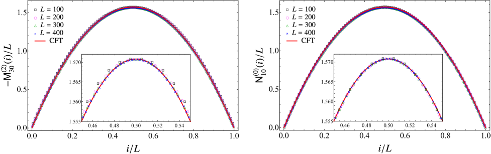
Since analytic results for the functions and are not available, we study the weight functions , , and in (49) by performing a numerical analysis of the combinations of the matrix elements of and defining them, which are given respectively by (36), (46), (39) and (42). These combinations depend on the number of sites in the interval and on the parameter labelling the number of diagonals to include in the sums. As already remarked above, we study the continuum limit by taking first, in order to guarantee that the functions and in (20) are well defined, and then . This means that we must keep in our numerical analysis. If we had analytic expressions for the functions and , we could check whether they vanish fast enough as to find convergence in the infinite sums defining the weight functions in (47) and (48), which occur in (49).
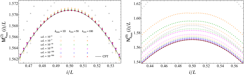
It is important to observe that, since (36), (39), (46) and (42) can be evaluated only in the spatial range given by , these combinations are not defined on the whole interval for finite values of and . The numerical results for these combinations are shown in the Appendix A (see the top panels in Fig. 15 and Fig. 16): they do not provide symmetric curves with respect to the center of the interval, as expected from the symmetry of the configuration, and they do not capture the CFT curve close to the right endpoint of the interval. This motivates us to employ decompositions of the operators and that are more suitable than (14) and (15) to obtain the CFT predictions on the entire interval. The decompositions (16) and (17) provide curves that are symmetric with respect to the center of the interval, but they do not allow to recover the CFT curve close to both the endpoints of the interval (see the middle panels in Fig. 15 and Fig. 16). In the following we consider the decompositions (2) and (2).
The procedure explained above to study the continuum limit of the entanglement hamiltonian can be adapted straightforwardly to the case where the decompositions (2) and (2) are employed. The result is again (49), with the weight functions given by (47) and (48). The crucial difference with respect to the previous analysis is that, as , in (47) we have with
| (50) |
and with
| (51) |
while in (48) we have with
| (52) |
and with
| (53) |
The occurrence of two branches in these functions of the spatial index (which originates from the splitting of the range in (2) and (2)) guarantees that they are well defined on the entire interval for finite values of . The combinations of diagonals in (50), (51), (52) and (53) display the symmetry under reflection with respect to the center of the interval, which has been observed also for the diagonals of and (see Fig. 2 and Fig. 3).
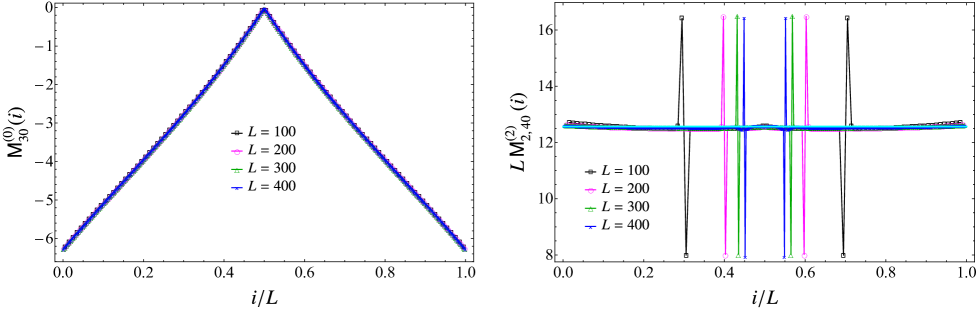
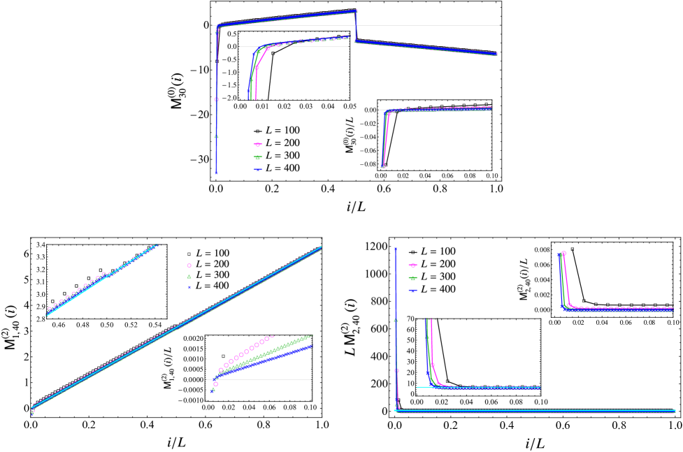
In Fig. 4 we show some numerical results for the combinations in (50) and (53). From the left panel we observe that, when is large enough, converges to a well defined function of . This observation allows to conclude that as at any given value of . Similarly, the data reported in the right panel of Fig. 4 show that, when is large enough, the product for increasing values of collapses on the horizontal line corresponding to except for four isolated and finite picks in each curve, whose positions depend on and whose heights are independent of . The positions of these picks are symmetric with respect to the center of the interval and they move towards the center of the interval as increases. These observations allow to conclude that as . Thus, the collapses of the data points observed in Fig. 4 for increasing values of lead to conclude that for the weight functions occurring in the term of (49) we should have
| (54) |
The curves in Fig. 4 are obtained through the decompositions (2) and (2). Considering the other decompositions reported in §2 and in Appendix A, one finds different curves, but all of them lead to the CFT prediction (54).
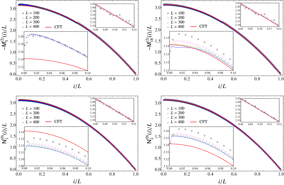
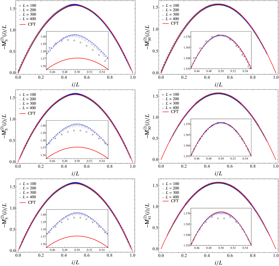
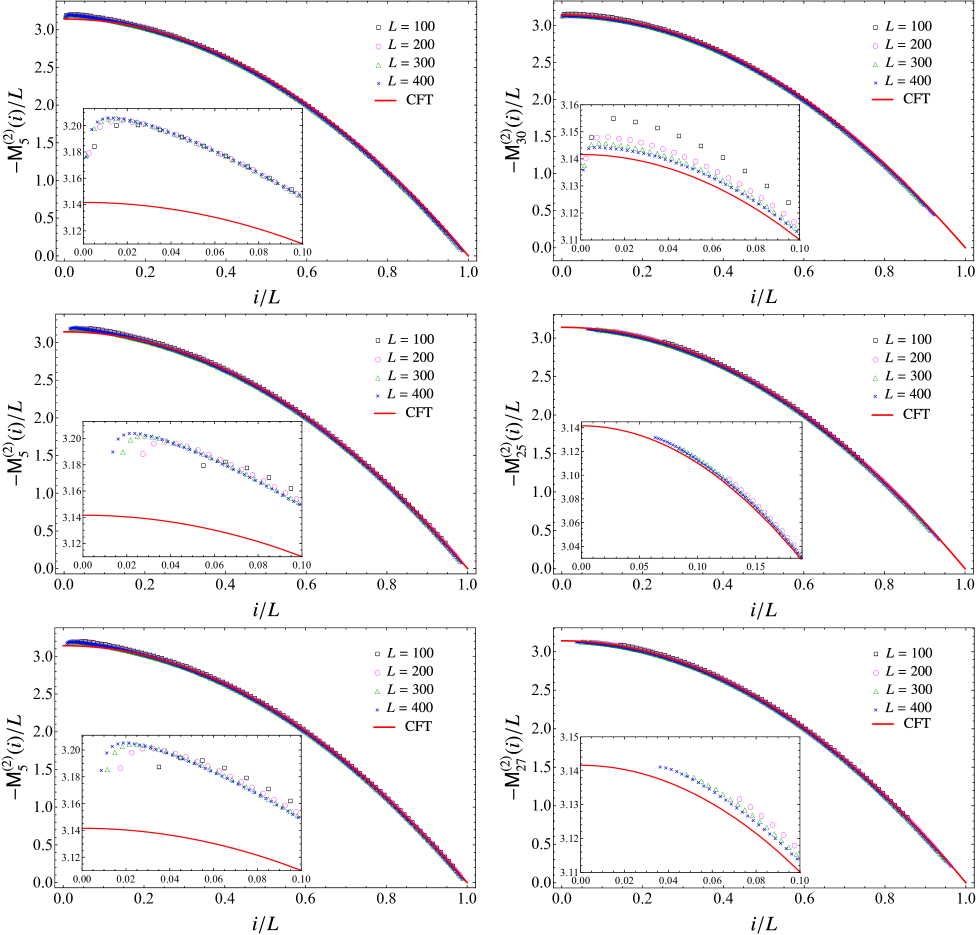
In Fig. 5 and Fig. 6
we report numerical results for the combinations in (51) and (52).
Comparing these two figures, it is straightforward to conclude
that the agreement between the numerical data and the CFT prediction
given by the parabola (3) (red solid curve)
improves as increases,
i.e. by including more diagonals in the sums occurring in
(51) and (52).
The data reported in Fig. 4 and Fig. 5
correspond to the optimal values of ,
when the behaviours of the data become stable.
These optimal values are different for the combinations involving and .
From Fig. 6
we also observe a parity effect in :
the asymptotic curve for a given
is either above or below the CFT curve,
depending on the parity of ,
and the distances between these curve decrease as increases
until the optimal value is reached.
We remark that the data points reported in
Fig. 4, Fig. 5 and Fig. 6
probe the entire interval ,
including the neighbourhoods of the endpoints.
Furthermore, the resulting curves are symmetric under
reflection with respect to the center of the interval,
as expected for this bipartition.
These features support our choice to employ the combinations
(50), (51),
(52) and (53).
The collapses of the data points in Fig. 5 for increasing values of lead to conjecture that the weight functions occurring in the finite term of (49) are
| (55) |
Thus, by employing the numerical results (54) and (55) into the expression (49) for the entanglement hamiltonian of an interval in the infinite line, we find the CFT prediction (2) with given by (3) and the energy density by (6).
We find it worth remarking that the height of the cyan horizontal line in the right panel of Fig. 4 corresponds to , being the weight function (3) predicted by CFT. A naive explanation of this observation comes from the fact that is a combination obtained through a finite differences approximation of (see (46)) and that the combination of provides in the continuum limit (see (55)). Nonetheless, an exchange of the second derivate of with the discrete sum over in (34) would provide an unexpected term containing multiplied by a constant weight function in the entanglement hamiltonian. This leads us to conclude that exchanges between derivatives with respect to and discrete sums over are not allowed.
3.3 Entanglement spectrum
In a two dimensional CFT, the entanglement spectra of an interval for the bipartitions shown in Fig. 1 have been studied in [13] through methods of Boundary Conformal Field Theory (BCFT) [25, 32, 33]. The occurrence of boundaries is due to the regularisation procedure, as briefly mentioned in §1. In the imaginary time description of the two dimensional spacetime underlying the bipartitions shown in Fig. 1, the UV cutoff can be introduced by removing an infinitesimal disk of radius around each entangling point [7, 18, 24, 13]. For the interval in the infinite line (left panel of Fig. 1), the remaining spacetime has two boundaries which encircle the two endpoints of the interval ; hence it can be mapped into an annulus through a conformal transformation. Given the symmetry of this bipartition with respect to the center of the interval, the same conformal boundary condition must be imposed on the two boundaries.
For harmonic chains in Gaussian states, standard techniques allow to evaluate the entanglement spectrum in terms of the single particle entanglement energies , which are obtained from the symplectic spectrum of the reduced covariance matrix of the subsystem [1, 2, 17, 27, 34]. Once the single particle entanglement energies have been ordered as , the gaps introduced in §1 can be written as linear combinations with non negative integer coefficients .
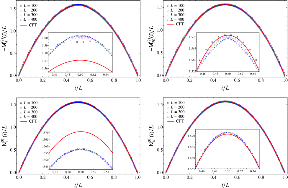
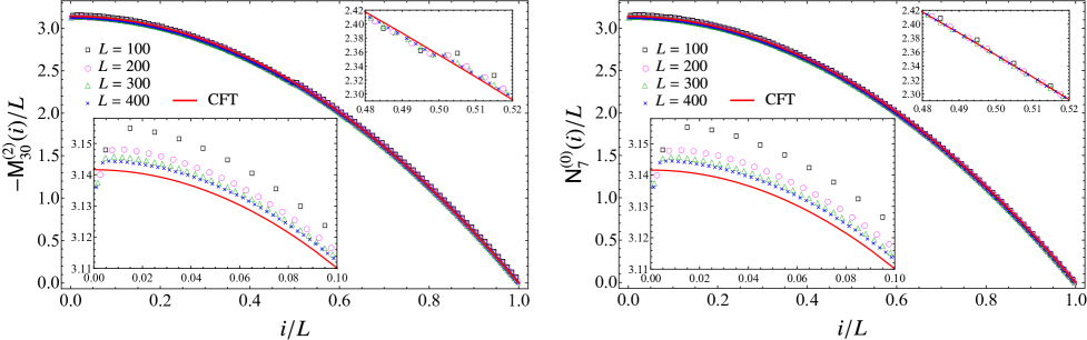
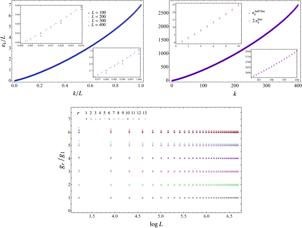
In the top left panel of Fig. 7, we report some numerical results for . For a given finite value of , we observe that as , while this does not happen for with . This leads us to assume that vanishes in the comparison of the numerical data with the CFT predictions in the bottom panel of Fig. 7. In the top right panel of Fig. 7 we show the single particle entanglement energies in terms of for some values of and, if is large enough, we find that the data having different collapse on a well defined curve, that would be interesting to obtain analytically. Given the above assumption about , in the bottom panel of Fig. 7 we show the numerical data for the ratios of the gaps with respect to the first gap as functions of . It is remarkable to observe that, as increases, the values of with collapse on all the integers with (we checked that when for the largest value of at our disposal). This originates from the fact that the single particle entanglement energies in the low-lying part of the spectrum are equally separated by a multiple integer of . Furthermore, the degeneracy of the -th level is given by the number of possible ways to partition the integer .
These numerical results for are compatible with the conformal spectrum of the BCFT given by a free massless scalar field on the segment with either Dirichlet or Neumann boundary conditions imposed on both the endpoints of the segment [33], but they cannot discriminate between these two possibilities. This ambiguity can be resolved by considering the entanglement spectrum of an interval at the beginning of a semi-infinite line with Dirichlet boundary conditions, that will be discussed in §4.3. In terms of the primary fields and of their descendants, we observe the towers of the identity and of .
The agreement found above with the spectrum of the BCFT of the free massless scalar field is expected only for the low-lying part of the entanglement spectrum.
4 Interval at the beginning of the semi-infinite line with Dirichlet b.c.
In this section we study the continuum limit of the entanglement hamiltonian of consecutive sites at the beginning of the massless harmonic chain on the semi-infinite line with Dirichlet boundary conditions at its endpoint. In §4.1 we find analytic expressions for the two-point correlators at a generic value of the mass parameter. Focussing on the massless regime, in §4.2 we adapt the procedure explained in §3 to this case, finding the CFT prediction (2), with the weight function (4) and the energy density (7). The continuum limit of the entanglement spectrum is discussed in §4.3.
4.1 Correlators
A finite harmonic chain in a segment with Dirichlet boundary conditions imposed at the endpoints is defined by (8) and by . The two-point correlators and in the ground state read respectively [35]
| (56) | |||||
| (57) |
where the dispersion relation is
| (58) |
In contrast with the harmonic chain in the infinite line (see §3.1), this harmonic chain is not translation invariant; hence the zero mode does not occur and the massless limit is well defined because the correlators (56) and (57) are finite.
In the thermodynamic limit, the correlators (56) and (57) can be written respectively as follows
| (59) | |||||
| (60) |
where and the Dirichlet boundary conditions are satisfied at the beginning of the semi-infinite line. We can evaluate the integrals (59) and (60) analytically by employing a prosthaphaeresis formula and an integral representation of the hypergeometric function111The following integral representation for the hypergeometric function has been employed in the special case given by and . . The final result reads
| (61) | |||||
| (62) |
where the functions are defined as follows
| (63) |
with and given by (27).
In the massless regime, which corresponds to , the expressions (61) and (62) significantly simplify and become the correlators found in [36], which are written in terms of the digamma function respectively as
| (64) | |||||
| (65) |
By restricting the indices and of the correlators (64) and (65) to the interval at the beginning of the semi-infinite line (see the right panel of Fig. 1), i.e. to the integer values in , we get the reduced correlation matrices and to employ in the expression (2) for the entanglement hamiltonian matrix . Plugging this matrix into (9), we can obtain the entanglement hamiltonian of the interval at the beginning of the semi-infinite line with Dirichlet boundary conditions imposed at its origin.
4.2 Entanglement hamiltonian
We are interested in the bipartition of the semi-infinite line whose origin coincides with the left endpoint of the interval made by sites (see the right panel of Fig. 1), when the entire system is in its ground state. The entanglement entropy of this bipartition has been studied for various systems e.g. in [8, 37]. In the massless harmonic chain with Dirichlet boundary conditions, the entanglement hamiltonian of this interval is given by (9) and (2), where the matrices and are the reduced correlation matrices introduced in §4.1 through the correlators (64) and (65). The result for the continuum limit predicted by CFT is (2), with the weight function given by (4) and the energy density (7) [29]. In the following we discuss a numerical procedure to obtain this CFT result.
The decompositions of the operators and introduced in §2 and in Appendix A naturally lead to consider the -th diagonals of the symmetric matrices and , like in the case of the interval in the infinite line discussed in §3.2. In the massless regime, we find numerical evidence that the limiting procedures defined in (20) provide well defined functions for any given value of . This is shown in Fig. 8 and Fig. 9 for the -th diagonal of the matrices and respectively, with . Notice that, while the functions and vanish at the entangling point that separates and , they are non vanishing at the beginning of the semi-infinite line, where the Dirichlet boundary condition is imposed. It would be interesting to find analytic expressions for these functions. Like for the interval in the infinite line, these functions have a well defined sign given by the parity of and the absolute value of their maximum significantly decreases as increases.
Assuming the existence of the functions and defined in (20), the continuum limit of the entanglement hamiltonian (12) can be studied by adapting to the bipartition that we are considering the procedure described in §3. Special care must be devoted to the boundary terms due to the integrations of a total derivative or to the integrations by parts. In particular, in (34) the integrand of the term is the total derivative , whose integral over the interval gives the boundary terms . These boundary terms vanish because at the entangling point and the Dirichlet boundary condition is imposed at the beginning of the semi-infinite line, where . The remaining expression reads
| (66) | |||
where terms have been discarded and has been introduced in (35).
The term in (66) is similar to the term in (34) and the terms containing and can be treated as discussed in §3.2. As for the term whose integrand is , we approximate through finite differences by writing because analytic expressions for are not known. Combining this approximation with (20) and (66), we are naturally led to introduce
| (67) |
and
| (68) |
being
| (69) |
where the subindex means that these quantities are related to the first derivative of the functions . Taking in (68), we find
| (70) |
Notice that we can also follow the steps performed in §3.2 combining the last two terms within the square brackets in (66) into and integrating by parts the corresponding integral, which provides the boundary terms . These terms do not contribute because at the entangling point and the Dirichlet boundary condition holds at the beginning of the semi-infinite line.
Taking the limit in (66) and employing the weight functions introduced in (47), (48) and (70), for the non vanishing contributions to the continuum limit of the entanglement hamiltonian we find
| (71) | |||||
We remark that, although some formal expressions occur also in the case of the interval in the infinite line in §3.2, their values depend on the system that we are exploring through the correlators (64) and (65).
Also in the numerical analysis of this bipartition we have employed all the decompositions introduced in §2 and in Appendix A as starting point. We find that the most effective approach is based on (50), (51), (52) and (53). For the interval at the beginning of the semi-infinite line, we also need the combination of the matrix elements of for and it is not difficult to find that it reads
| (72) |
Like for the interval in the infinite line, the occurrence of two branches in (50), (51), (52) (53) and (72) allows to probe the entire interval. This cannot be done when the decompositions (14) and (15) are employed (see top panels of Fig. 17 and Fig. 18). Notice that, in contrast with §3.2, in this case the reflection symmetry with respect to the center of the interval is not expected.
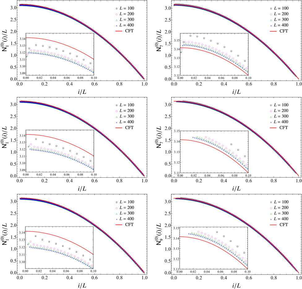
In Fig. 10 we observe that the numerical data for , and with collapse on well defined curves when increases. As for some of the weight functions occurring in (71), these collapses support the following conjecture
| (73) |
for any fixed value of such that . The insets on the right in all the panels of Fig. 10 highlight that the values of , and for seem to converge to finite non vanishing constants. Since , and are multiplied by in (71), the Dirichlet boundary condition implies that this feature does not provide a non vanishing term in the continuum limit of the entanglement hamiltonian. In the top panel of Fig. 10, the discontinuity in the center of the interval is due to the fact that in (50) is defined through two branches. This discontinuity is not observed if different decompositions for the operators and in (13) are adopted.
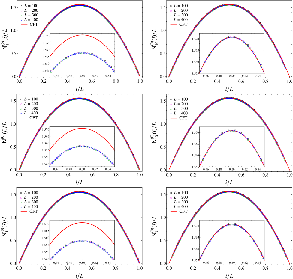
In Fig. 11 we show (left panel) and (right panel) for increasing values of and an optimal value of which guarantee certain stability of the numerical results. The collapses of the data points naturally lead to conjecture that
| (74) |
where is the half parabola (4) predicted by the CFT. Comparing these results with the corresponding ones for the interval in the infinite line (see Fig. 5), we observe that larger values of are needed in this case to reach the CFT curve in the neighbourhood of the beginning of the semi-infinite line, which is sensible to the boundary conditions.
In the bottom panels of Fig. 10, the data points for and with collapse on the cyan straight lines, which correspond respectively to and to when is large enough. Similarly to the case of the interval in the infinite line (see the final remarks of §3.2), we can roughly justify this behaviour by noticing that and are obtained through finite differences approximations of and respectively; hence, from (74), one expects to find respectively and . Also in this case exchanging the derivatives with respect to with the discrete sums over leads to wrong results, as already discussed in the final part of §3.2 for the interval in the infinite line.
In Fig. 12 we show again and , but for lower values of in order to highlight the fact that the collapse of the numerical data onto the CFT curve improves as increases. This behaviour is stabilised around optimal values for that correspond to the data reported in Fig. 11. Furthermore, also in this case we encounter the same parity effect observed in Fig. 6 and mentioned in §3.2.
4.3 Entanglement spectrum
The BCFT analysis of the entanglement spectrum presented in [13], where (5) has been derived, includes the case that we are considering, given by the entire system in its ground state and the interval at the beginning of the semi-infinite line. In this bipartition only one entangling point occurs; hence the UV cutoff is introduced by removing only a disk of radius around the entangling point. The resulting euclidean spacetime has the topology of the annulus and in this case different conformal boundary conditions are allowed at the two boundaries. In our analysis we impose Dirichlet boundary conditions along the boundary corresponding to the beginning of the semi-infinite line.
The numerical analysis of the entanglement spectrum is performed like in §3.3 and the crucial difference with respect to the interval in the infinite line is that the massless regime given by is well defined. In this regime we observe that the lowest single particle entanglement energy is non vanishing, in contrast with the case of the interval in the infinite line.
In the top left panel of Fig. 13 we show the numerical results for the single particle entanglement energies in terms of corresponding to some values of , finding that they nicely collapse on a well defined curve when is large enough, like in the case of the interval in the infinite line (see the top right panel of Fig. 7). The curves obtained for these two spatial bipartitions are compared in the top right panel of Fig. 13, finding that they basically overlap, once the curve for the interval in the infinite line is multiplied by a factor of (the insets highlight that this agreement is very good in the highest part of the spectrum and gets worse in the lowest part of the spectrum).
In the bottom panel of Fig. 13 we show the ratios between the generic gap and the smallest gap in the entanglement spectrum as functions of , for . These ratios take all the integer values between and included (we checked that for for the largest value of at our disposal). This feature originates from the fact that in the low-lying part of the single particle entanglement spectrum the eigenvalues are equally separated by an integer multiple of (see also §3.3). Comparing Fig. 13 and Fig. 7, it is straightforward to notice that take all the integer values for both the bipartitions, but the corresponding degeneracies are very different in the two cases. In particular, in Fig. 13 the degeneracy of the -th level is given by the number of partitions of that do not contain repeated positive integers.
The degeneracy observed in Fig. 13 is compatible with the conformal spectrum of the free massless scalar on a segment with mixed boundary conditions, namely with Dirichlet boundary conditions imposed at one endpoint and Neumann boundary conditions at the other endpoint [33]. Since in our analysis Dirichlet boundary conditions are imposed at the beginning of the semi-infinite line, we can conclude that Neumann boundary conditions must be imposed at the boundary introduced by the regularisation procedure around the entangling point. This allows to fix the ambiguity found in §3.3, concluding that the numerical results for the entanglement spectrum of the interval in the infinite line in the continuum limit agree with the conformal spectrum of the BCFT given by the free massless scalar on a segment with Neumann boundary conditions imposed on both the boundaries encircling the endpoints of the interval in the euclidean spacetime. Also for this bipartition we expect that the agreement with the conformal spectrum of the BCFT holds only for the low-lying part of the entanglement spectrum.
5 Conclusions
In this manuscript we have performed a numerical analysis of the continuum limit of the entanglement hamiltonians of a block made by consecutive sites in massless harmonic chains, in the two cases where the subsystem is an interval in the infinite line or an interval at the beginning of the semi-infinite line with Dirichlet boundary conditions imposed at its endpoint. The procedure is based on the method introduced in [20, 22] for chains of free fermions, which has been adapted here to harmonic chains.
We have obtained the analytic expression (2) predicted by CFT, with the weight function and the energy density respectively given by (3) and (6) for the interval in the infinite line and by (4) and (7) for the interval at the beginning of a semi-infinite line. A remarkable agreement between the data points and the weight functions predicted by CFT is observed (see Fig. 5 and Fig. 11). It would be instructive to support our numerical results with analytic computations, by first finding analytic expressions for the functions and (see Fig. 2, Fig. 3 for the interval in the infinite line and Fig. 8 and Fig. 9 for the interval at the beginning of the semi-infinite line) and then by performing analytically the sums involving these functions and their derivatives which provide continuum limit of the entanglement hamiltonians, as done in [20, 22] for the interval in the infinite chain of free fermions.
We have also explored the continuum limit of the entanglement spectra of these entanglement hamiltonians, finding that the ratios of the low-lying gaps provide the ratios of the conformal dimensions of the BCFT given by the massless scalar on the annulus with the proper conformal boundary conditions, as predicted in [13] (see Fig. 7 and Fig. 13). The numerical results indicate that Neumann boundary conditions must be imposed along the boundaries introduced by the regularisation procedure. This is in agreement with a similar numerical analysis performed in lattice spin models [26], where it has been found that the numerical results for the entanglement spectra are compatible with the conformal spectra of BCFT with free boundary conditions imposed along the boundaries around the entangling points. This has been confirmed also by numerical studies out of equilibrium [28].
The results reported in this manuscript can be extended in various directions. In massless harmonic chains, the entanglement hamiltonians of an interval in a circle when the system is in its ground state or in the infinite line when the system is at finite temperature should be studied because in these cases (2) still holds and the weight functions are known from CFT [12, 13, 21, 22]. It is also natural to explore the entanglement hamiltonians for bipartitions involving disjoint intervals [38, 15, 16], spatially inhomogeneous chains [39, 14] and higher dimensional quantum systems [11]. It is important to find explicit expressions for the entanglement hamiltonians in interacting lattice models, both through analytic and numerical methods [41, 42, 40, 43, 44]. Also the analysis of the entanglement spectra [26, 45, 46, 48, 47, 34] and of the contour for the entanglement entropies [30, 49, 50], which is a quantity strictly related to the entanglement hamiltonian, deserve further analysis. It is useful also to study operators on the lattice that provides efficient approximations of the entanglement hamiltonians [14, 51]. We also mention that, in order to understand the unitary time evolution of a system after a quantum quench, i.e. after a sudden change that drives the system out of equilibrium [52], relevant insights could come from the analysis of the time evolutions of the entanglement hamiltonians and of their entanglement spectra [13, 53, 27, 28, 55, 54].
Acknowledgements
It is our pleasure to thank Raúl Arias, Viktor Eisler, Mihail Mintchev and Ingo Peschel for important comments. We are grateful also to Vincenzo Alba, John Cardy, Paul Fendley, Andreas Ludwig, Giuseppe Mussardo, German Sierra, Jacopo Surace and Luca Tagliacozzo for useful discussions. ET acknowledges the Yukawa Institute for Theoretical Physics at Kyoto University (workshop YITP-T-19-03 Quantum Information and String Theory 2019) and the Instituto de Física Teórica (Madrid) for financial support and warm hospitality during part of this work.
Appendices
Appendix A Alternative summations and role of
In this Appendix we report further results supporting the numerical analysis discussed in the main text. First we briefly discuss the choice of the numerical value of adopted to study the entanglement hamiltonian of the interval in the infinite line. In the remaining part of this Appendix, we discuss some numerical results obtained through decompositions of the operators and in (13) that are different from (2) and (2).
The harmonic chain on the infinite line displays translation invariance and this symmetry leads to the occurrence of the zero mode, that prevents us to set in our numerical analysis, as already remarked in §3.1. In order to study the entanglement hamiltonians in the massless regime of this harmonic chain, we have to choose very small but non vanishing values of . The high numerical precision required for our numerical analysis allows to take significantly close to zero. The numerical data reported in the figures discussed in §3.2 and §3.3 correspond to and in Fig. 14 we justify this choice by showing and for decreasing values of and for three increasing values of at fixed . In order to find a small value for that properly captures the features of the massless regime, we require that the numerical data are stabilised on the CFT prediction (3) for different values of . While this condition is fulfilled already for in the left panel of Fig. 14, it is not satisfied in the right panel. Instead, for very good collapses on the CFT curve are observed for the data corresponding to different .
In the main text we have discussed the results for the continuum limit reported in Fig. 4 and Fig. 5 for the interval in the infinite line (see §3.2) and in Fig. 10 and Fig. 11 for the interval at the beginning of the semi-infinite line (see §4.2). They have been obtained by starting from the decompositions (2) and (2) for and , which lead to the combinations (50), (51), (52) and (53) for the interval in the infinite line, and to the same combinations together with (72) for the interval at the beginning of the semi-infinite line.
The procedure to study the continuum limit starting from the decompositions (14) and (15) for and , which provides the combinations (36), (39), (42) and (46) for the interval in the infinite line (see §3.2) and the same combinations together with (67) for the interval at the beginning of the semi-infinite line (see §4.2), has been explained in the main text. The numerical results of the combinations (42) and (39) for various sizes of the intervals and for two values of are shown in the top panels of Fig. 15 and Fig. 16 for the interval in the infinite line and of Fig. 17 and Fig. 18 for the interval at the beginning of the semi-infinite line. As increases, the agreement between the data and the CFT predictions given by (3) and (4) improves. The numerical data stabilise around a value that has been adopted in the right panels. As for the combinations (36) and (46), we find that they lead to the function that vanishes identically in the interval, as expected from CFT. The range of the index in these combinations do not allow to capture the curve predicted by CFT on the entire interval and this fact motivated us to employ the decompositions (2) and (2) instead of (14) and (15).
In the remaining part of this Appendix, we discuss the continuum limit of the entanglement hamiltonians based on two other decompositions for and in (13).
Considering the decompositions (16) and (17), by adapting the procedure described in §3.2, we find the combinations given by
| (75) |
and
| (76) |
where . We emphasise that the combinations (75) have been found also in [19] by employing a different approach. The data obtained through the combinations (75) are shown in the middle panels of Fig. 15 and Fig. 16 for the interval in the infinite line and of Fig. 17 and Fig. 18 for the interval at the beginning of the semi-infinite line. Also in this case the agreement with the CFT predictions (3) and (4) improves as increases until it reaches an optimal value corresponding to the one adopted in the right panels. Comparing the middle panels with the top panels and with Fig. 5, Fig. 6, Fig. 11 and Fig. 12, it is straightforward to notice that (75) do not allow to describe the CFT curves close to both the endpoints of the interval. The data corresponding to (76), that are not reported in this manuscript, provide the function that vanish identically in the interval as increases and for optimal values of , as expected from the CFT analysis.
Another way to obtain the results predicted by CFT in the continuum limit can be introduced by adapting the method employed in the numerical analysis of [22] for the entanglement hamiltonian of an interval in an infinite chain of free fermions. Considering only blocks containing an even number of sites, let us decompose the operators and in (13) respectively as
| (77) | |||
and
| (78) | |||
where we have separated the contributions of the even diagonals of and from the contributions of the odd diagonals.
In (77) and (78) the index labels the elements along the diagonals of and , while in the decompositions introduced in §2 it corresponds to a row index. Treating separately the contributions of the odd diagonals and of the even diagonals in (77) and (78) and using (29), (30) and (31), we can adapt the procedure described in §3.2 to these decompositions of the operators and . In this case we find that the combinations of diagonals occurring at the leading order as are
| (79) |
which come from the even and odd diagonals respectively.
The next subleading order in the expansion of the entanglement hamiltonian as gets contributions both from and . In particular, the continuum limit of to this order gives
| (80) |
and the term originated from the finite difference approximation of , namely
| (81) | |||
while from we find only
| (82) |
Notice that the range of the index in the above expression is for the combinations coming from the odd diagonals and for the combinations coming from the even diagonals.
The final expressions providing the continuum limit of the entanglement hamiltonian are proper combinations of the terms coming from the even and odd diagonals, but in constructing these combinations we encounter the problem that the former ones are defined on sites, while in the latter ones the index assumes values. In this case the index labels the elements along the diagonals; hence, focussing e.g. on (80), we encounter an ambiguity in the way to combine with . In the following, first we split as , with . Then, in the sum between the even and the odd part, we choose to associate to and to . The values of and are not fixed uniquely and we choose in our numerical analysis. For the interval in the infinite line, this choice guarantees the expected symmetry with respect to the center of the interval at finite .
By applying this procedure to all the expressions in (79), (80), (81) and (82), we obtain respectively
| (83) | |||||
| (84) | |||||
| (85) | |||||
| (86) |
where and we have employed the parameter adopted throughout all this manuscript to label the last diagonal occurring in a particular combination of diagonals. Since we always choose odd in our numerical analysis, the same number of even and odd diagonals occurs in the above combinations.
The numerical results for (84) and (86) are reported respectively in the left and right bottom panels of Fig. 15 and Fig. 16 for the interval in the infinite line and of Fig. 17 and Fig. 18 for the interval at the beginning of the semi-infinite line. As and increase, with , we observe again that the agreement of the numerical data with the CFT curves (3) and (4) improves. Nonetheless, since , the data points cannot capture the CFT curves close to the endpoints of the interval. We have also checked that, by performing this numerical analysis for (83) and (85), the vanishing curve is obtained everywhere within the interval except in the left endpoint in the case of the semi-infinite, where the Dirichlet boundary conditions are imposed. Also these results confirm the CFT predictions.
References
References
- [1] I. Peschel and V. Eisler, J. Phys. A 42, 504003 (2009).
- [2] H. Casini and M. Huerta, J. Phys. A 42, 504007 (2009).
-
[3]
L. Amico, R. Fazio, A. Osterloh and V. Vedral,
Rev. Mod. Phys. 80, 517 (2008);
P. Calabrese and J. Cardy, J. Phys. A 42 504005 (2009);
J. Eisert, M. Cramer, M.B. Plenio Rev. Mod. Phys. 82, 277 (2010). -
[4]
T. Nishioka, S. Ryu and T. Takayanagi,
J. Phys. A 42, 504008 (2009);
M. Rangamani and T. Takayanagi, Lect. Notes Phys. 931 (2017). -
[5]
R. Islam, R. Ma, P. Preiss, M. Tai, A. Lukin, M. Rispoli and M. Greiner,
Nature 528, 77 (2015);
A. Kaufman, M. Tai, A. Lukin, M. Rispoli, R. Schittko, P. Preiss and M. Greiner, Science 353, 794 (2016). -
[6]
L. Bombelli, R. Koul, J. Lee and R. Sorkin,
Phys. Rev. D 34, 373 (1986);
M. Srednicki, Phys. Rev. Lett. 71, 666 (1993);
C. Callan and F. Wilczek, Phys. Lett. B 333 (1994). - [7] C. Holzhey, F. Larsen and F. Wilczek, Nucl. Phys. B 424, 443 (1994).
- [8] P. Calabrese and J. Cardy, J. Stat. Mech. P06002 (2004).
-
[9]
J. Bisognano and E. Wichmann,
J. Math. Phys. 16, 985 (1975);
J. Bisognano and E. Wichmann, J. Math. Phys. 17, 303 (1976). - [10] P. Hislop and R. Longo, Comm. Math. Phys 84, 71 (1982).
- [11] H. Casini, M. Huerta and R. Myers, JHEP 1105:036 (2011).
- [12] G. Wong, I. Klich, L. Pando Zayas and D. Vaman, JHEP 1312:020 (2013).
- [13] J. Cardy and E. Tonni, J. Stat. Mech. 123103 (2016).
- [14] E. Tonni, J. Rodríguez-Laguna and G. Sierra, J. Stat. Mech. 043105 (2018).
-
[15]
H. Casini and M. Huerta,
Class. Quant. Grav. 26, 185005 (2009);
R. Longo, P. Martinetti and K.-H. Rehren, Rev. Math. Phys. 22, 331 (2010). - [16] R. Arias, H. Casini, M. Huerta and D. Pontello, Phys. Rev. D 98, 125008 (2018).
-
[17]
I. Peschel and M. Chung,
J. Phys. A 48, 8419 (1999);
M. Chung and I. Peschel, Phys. Rev. B 62, 4191 (2000);
M. Chung and I. Peschel, Phys. Rev. B 64, 064412 (2001);
I. Peschel, J. Phys. A 36, L205 (2003);
S. Cheong and C. Henley, Phys. Rev. B 69, 075112 (2004);
V. Eisler, D. Karevski, T. Platini and I. Peschel, J. Stat. Mech. P01023 (2008);
V. Eisler and I. Peschel, J. Stat. Mech. P04028 (2013);
R. Arias, H. Casini, M. Huerta and D. Pontello, Phys. Rev. D 96, 105019 (2017). - [18] I. Peschel, J. Stat. Mech. P06004 (2004).
- [19] R. Arias, D. Blanco, H. Casini and M. Huerta, Phys. Rev. D 95, 065005 (2017).
- [20] V. Eisler and I. Peschel, J. Phys. A: Math. Theor. 50, 284003 (2017).
- [21] V. Eisler and I. Peschel, J. Stat. Mech. 104001 (2018).
- [22] V. Eisler, E. Tonni and I. Peschel, J. Stat. Mech. (2019) 073101.
- [23] H. Li and F. D. M. Haldane, Phys. Rev. Lett. 101, 010504 (2008).
- [24] K. Ohmori and Y. Tachikawa J. Stat. Mech. 1504 (2015) P04010.
-
[25]
J. Cardy,
Nucl. Phys. B 275, 200 (1986);
J. Cardy, Nucl. Phys. B 324, 581 (1989);
H. Saleur and M. Bauer, Nucl. Phys. B 320 (1989) 591;
J. Cardy, Conformal Invariance and Statistical Mechanics, lectures delivered at Les Houches 1988;
J. Cardy, arXiv:hep-th/0411189. - [26] A. Läuchli, arXiv:1303.0741.
- [27] G. Di Giulio, R. Arias and E. Tonni, arXiv:1905.01144.
- [28] J. Surace, L. Tagliacozzo and E. Tonni, arXiv:1909.07381.
- [29] A. Liguori and M. Mintchev, Nucl. Phys. B 522, 345 (1998).
- [30] A. Botero and B. Reznik, Phys. Rev. A 70, 052329 (2004).
- [31] A. Altland and B. Simons, Condensed Matter Field Theory, Cambridge University Press (2010).
-
[32]
C. Callan and I. Klebanov,
Phys. Rev. Lett. 72, 1968 (1994);
C. Callan, I. Klebanov, A. Ludwig and J. Maldacena, Nucl. Phys.B 422, 417 (1994). - [33] R. Blumenhagen and E. Plauschinn, Introduction to Conformal Field Theory, Springer (2009).
- [34] B. Herwerth, G. Sierra, J. Cirac and A. Nielsen, Phys. Rev. B 98, 115156 (2018).
- [35] S. Lievens, N. Stoilova and J. Van der Jeugt, J. Math. Phys. 49, 073502 (2008).
- [36] P. Calabrese, J. Cardy and E. Tonni, J. Stat. Mech. P02008 (2013).
- [37] L. Taddia, J. Xavier, F. Alcaraz, and G. Sierra, Phys. Rev. B 88, 075112 (2013).
-
[38]
S. Furukawa, V. Pasquier and J. Shiraishi,
Phys. Rev. Lett. 102, 170602 (2009);
M. Caraglio and F. Gliozzi, JHEP 0811:076 (2008);
P. Calabrese, J. Cardy and E. Tonni, J. Stat. Mech. P11001 (2009);
M. Fagotti and P. Calabrese, J. Stat. Mech. P04016 (2010);
P. Calabrese, J. Cardy and E. Tonni, J. Stat. Mech. P01021 (2011);
V. Alba, L. Tagliacozzo and P. Calabrese, J. Stat. Mech. P06012 (2011);
J. Cardy, J. Phys. A 46, 285402 (2013);
A. Coser, L. Tagliacozzo and E. Tonni, J. Stat. Mech. P01008 (2014);
C. De Nobili, A. Coser and E. Tonni, J. Stat. Mech. P06021 (2015);
A. Coser, E. Tonni and P. Calabrese, J. Stat. Mech. 053109 (2016). -
[39]
N. Allegra, J. Dubail, J. Stéphan and J. Viti,
J. Stat. Mech. 053108 (2016);
J. Dubail, J. Stéphan, J. Viti and P. Calabrese, SciPost Phys. 2, 002 (2017). - [40] B. Nienhuis, M. Campostrini and P. Calabrese, J. Stat. Mech. P02063 (2009).
-
[41]
I. Peschel and T. Truong,
Z. Phys. B - Condensed Matter 69, 385 391 (1987);
H. Itoyama and H. Thacker, Phys. Rev. Lett. 58, 1395 (1987);
I. Peschel, M. Kaulke and O. Legeza, Ann. Phys. 8, 153 (1999). - [42] F. Parisen Toldin and F. Assaad, Phys. Rev. Lett. 121, 200602 (2018).
- [43] G. Cho, A. Ludwig and S. Ryu Phys. Rev. B 95, 115122 (2017).
-
[44]
I. Klich, D. Vaman and G. Wong,
Phys. Rev. Lett. 119, 120401 (2017);
I. Klich, D. Vaman and G. Wong, Phys. Rev. B 98, 035134 (2018);
G. Wong, JHEP 2019:45 (2019);
D. Blanco and G. Perez-Nadal, Phys. Rev. D 100, 025003 (2019);
P. Fries and I. Reyes, arXiv:1905.05768;
D. Blanco, A. Garbarz and G. Perez-Nadal, JHEP 2019:76 (2019). - [45] P. Calabrese and A. Lefevre, Phys. Rev A 78, 032329 (2008).
- [46] V. Alba, M. Haque and A. Läuchli, Phys. Rev. Lett. 108, 227201 (2012).
-
[47]
F. Assaad, T. Lang and F. Parisen Toldin,
Phys. Rev. B 89, 125121 (2014);
F. Assaad Phys. Rev B 91, 125146 (2015). - [48] V. Alba, P. Calabrese and E. Tonni, J. Phys. A 51, 024001 (2018).
- [49] Y. Chen and G. Vidal, J. Stat. Mech. P10011 (2014).
- [50] A. Coser, C. De Nobili and E. Tonni, J. Phys. A 50, 314001 (2017).
-
[51]
M. Dalmonte, B. Vermersch and P. Zoller,
Nature Physics 14, 827–831 (2018);
G. Giudici, T. Mendes-Santos, P. Calabrese and M. Dalmonte, Phys. Rev. B 98, 134403 (2018);
T. Mendes-Santos, G. Giudici, M. Dalmonte and M. Rajabpour, Phys. Rev. B 100, 155122 (2019). -
[52]
P. Calabrese and J. Cardy,
J. Stat. Mech. P04010 (2005);
P. Calabrese and J. Cardy, Phys. Rev. Lett. 96, 136801 (2006);
P. Calabrese and J. Cardy, J. Stat. Mech. P06008 (2007). - [53] G. Torlai, L. Tagliacozzo and G. De Chiara, J. Stat. Mech. P06001 (2014).
- [54] X. Wen, S. Ryu and A. Ludwig, J. Stat. Mech. 113103 (2018).
- [55] W. Zhu, Z. Huang, Y. He and X. Wen, arXiv:1909.08808.