Towards the Automation of Deep Image Prior

Abstract

Single image inverse problem is a notoriously challenging ill-posed problem that aims to restore the original image from one of its corrupted versions. Recently, this field has been immensely influenced by the emergence of deep-learning techniques. Deep Image Prior (DIP) offers a new approach that forces the recovered image to be synthesized from a given deep architecture. While DIP is quite an effective unsupervised approach, it is deprecated in real-world applications because of the requirement of human assistance.

In this work, we aim to find the best-recovered image without the assistance of humans by adding a stopping criterion, which will reach maximum when the iteration no longer improves the image quality. More specifically, we propose to add a pseudo noise to the corrupted image and measure the pseudo-noise component in the recovered image by the orthogonality between signal and noise. The accuracy of the orthogonal stopping criterion has been demonstrated for several tested problems such as denoising, super-resolution, and inpainting, in which 38 out of 40 experiments are higher than 95%.

1 Introduction

Image inverse problem center around the recovery of an unknown image $x$ based on given corrupted measurement $y$. It is an ill-posed problem because a specific corrupted image $y$ can correspond to a crop of possible high-quality images. The problem has been extensively explored in the past several decades while deep convolutional neural networks (ConvNets) currently set the state-of-the-art [11], such as denoising [2], or single-image super-resolution [4]. The commonly suggested and very effective path to the inverse problem is as follows: Given many example of pairs of an original image and its corrupted version, one could learn a deep network to match the degraded image to its source [7], for example, [14, 16, 5, 9, 6, 8, 17, 13, 10, 3].

Ulyanov et al. [11] proposed a new strategy, namely Deep Image Prior (DIP), for a single image inverse problem where common strategies are on longer feasible because only one corrupted image (without the original image) is available for model training. Mataev et al. [7] further improved the performance of the DIP by adding an extra regularization (Regularization by Denoising).

Although Ulyanov et al. [11] and Mataev et al. [7] proofed that DIP and its variations are very effective machines for handling various inverse problems, we have to figure out a stopping method before applying DIPs to real-world problems where human supervision is not available. Currently, DIPs stop when humans assess their outputs as good enough or reach their maximum iteration times [11, 7]. The stopping method should output a measurement that indicates how well DIPs have reconstructed the interested image. So, the training algorithm can stop itself when the measurement reaches the maximum.

In this work, we propose a stopping method, namely Orthogonal Stopping Criterion (OSC), which adds a pseudo noise to the corrupted image and measure the pseudo-noise component in the recovered image of each iteration based on the orthogonality between signal and noise. The growth-rate derivate of the measurement will reach its maximum when DIPs start focusing on reconstructing the pseudo noise, which means the training should be stopped because DIPs resist "bad" solutions and descends much more quickly towards naturally-looking images [11]. We use DIP as the baseline and have demonstrated the performance of OSC for several problems such as denoising, super-resolution, inpainting.

2 Methodology

The inverse tasks such as denoising, super-resolution and inpainting can be expressed as energy minimization problem of equation (1), where $E(x;x_{0})$ is a task-dependent data term, $x_{0}$ is the noisy/low-resolution/occluded image, $x$ is the reconstructed image, and $R(x)$ is a regularizer [11].

$$x^{*} =\arg\min_{x}E(x;x_{0})+R(x)$$ (1)

In this work, we handle the inverse tasks by equation (2) where $pn$ is the pseudo noise and all $x$ that we get during the minimization are represented as set $\mathbb{X}$. The minimization is stopped according to equation (3), where $O(x;pn)$ measures the growth-rate derivate of the pseudo-noise component in $x$. The pseudo-noise component is highly correlate to $pn$, because $pn$ is orthogonal to all components in $x_{0}$ including ground truth and corruptions. Since the reconstruction of $pn$ needs much more iterations than the naturally-looking image in $x_{0}$, the interested naturally-looking image will be reconstructed by DIP before the growth-rate derivate of the pseudo-noise component reaches its maximum, as long as the reconstruction difficulty of $pn$ is harder than the naturally-looking image and easier than (or equal to) other corruptions.

$$\min_{x}E(x;x_{0}+pn)+R(x)$$ (2)

$$x^{*} =\arg\max_{x}O(x;pn),x\in\mathbb{X}$$ (3)

Given a series of reconstructed images $x_{i},i=1,2,3,...$, we get the pseudo noise component $e_{i}$ by equation (4), where $N$ is the number of elements in $x_{i}$ and $i$ indicates the image which is reconstructed in the $i$th iteration.

$$e_{i} =\frac{1}{N}\sum_{j=1}^{N}x_{i,j}\times pn_{j}$$ (4)

We get the index $i^{*}$ of the best image by equation (5) where $C(e_{i})$ finds the curvature of the $e_{i}$ curve. Figure 1 has shown the results of F16 denoising experiment, including the $e_{i}$ curve, the Peak Signal to Noise Ratio (PSNR) curve of DIP, the PSNR curve of OSC, and curvature curves. All curves are normalized according to their own minimum and maximum except the PSNR curve of OSC which uses the minimum and the maximum of the DIP PSNR curve. The curvature curve records the growth-rate derivate of the $e_{i}$ curve. To get the curvature curve, for a specific $i$, we find 3 points on the $e_{i}$ curve to define the new coordinate system shown in dash line, which are $(x_{1},y_{1})$, $(x_{2},y_{2})$, $(x_{3},y_{3})$ where $x_{1}=i-H$, $y_{1}=mean(e_{m_{1}})$, $m_{1}\in[i-H-h,i-H+h]$, $x_{2}=i$, $y_{2}=mean(e_{m_{2}})$, $m_{2}\in[i-h,i+h]$, $x_{3}=i+H$, $y_{3}=mean(e_{m_{3}})$, $m_{3}\in[i+H-h,i+H+h]$. $H$ defines the length of $e_{i}$ curve for curvature calculation. $h$ is the averaging window size. After mapping the $e_{i}$ curve between $(x_{1},y_{1})$ and $(x_{3},y_{3})$ to the dash-line coordinate system, we fit a parabola to the curve and use the parameter of the quadratic item as the curvature at index $i$ which is an approximation of the growth-rate derivate of the pseudo-noise component. From Figure 1, although the curvature-maximum PSNR is not the maximum one during the whole OSC iteration, it’s close enough that the ratios of the curvature-maximum PSNR to the maximum one are more than 95% in the most of our experiments. It is clear in Figure 1 that the existence of the pseudo noise will harm the maximum PSNR but it is insignificant. The OSC method has been listed in Algorithm 1.

$$i^{*} =\arg\max_{i}C(e_{i})$$ (5)

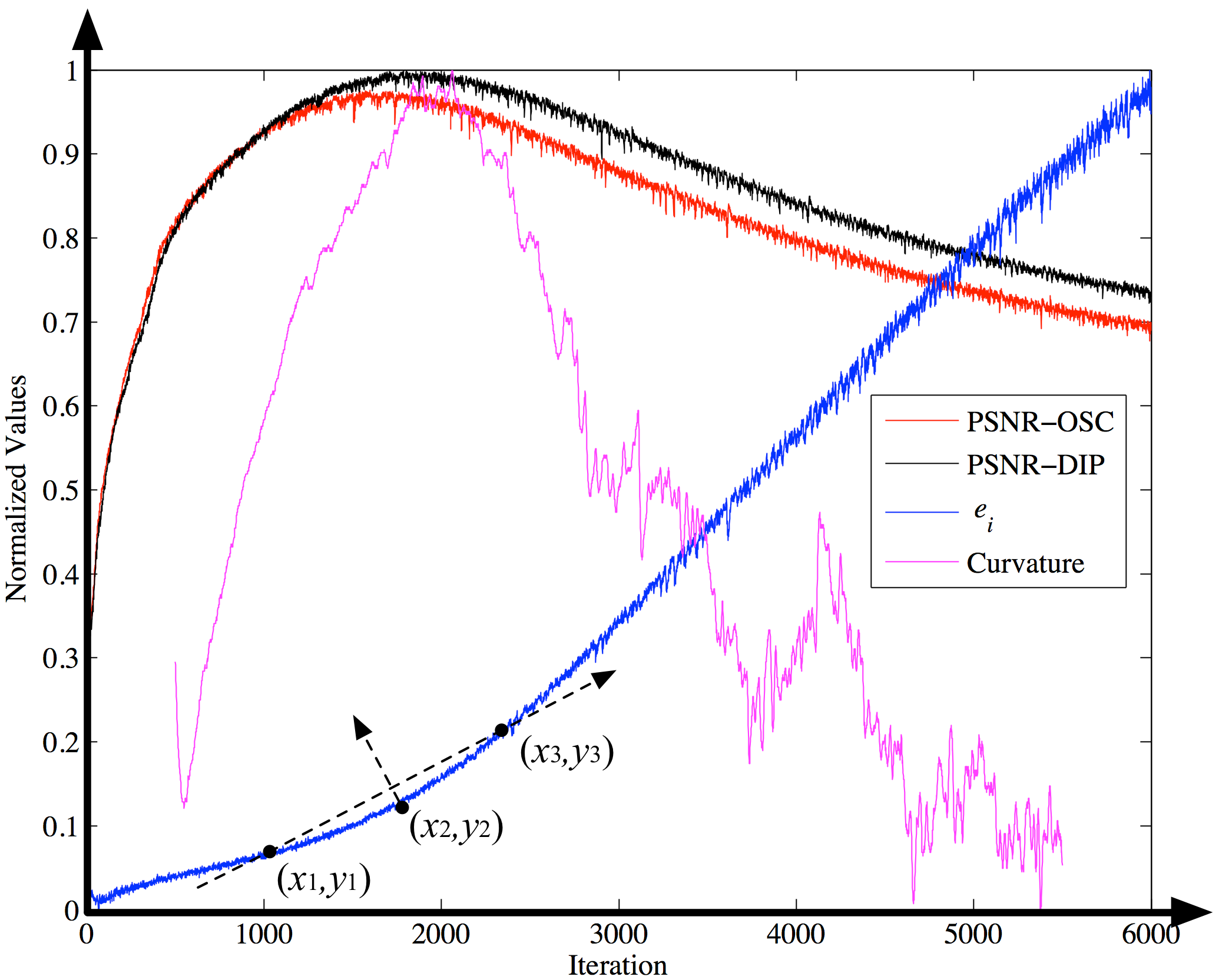
Figure 1: Example of the $e_{i}$ curve.

Algorithm 1 Orthogonal Stopping Criterion

0: Corrupted image $x_{0}$, half window length $H$ for curvature calculation, $h$ as the half window length for averaging.

0: The best index $i^{*}$ where the curvature-maximum PSNR has been reached.

1: Generate a pseudo noise $pn$.

2: for all $i$ do

3:    Try to minimize equation (2) and get a reconstructed image $x_{i}$

4:    Get the measurement of pseudo noise component by equation (4).

5:    Calculate the curvature at $j=i-H-h$ by $C(e_{j})$.

6: end for

7: return The index $i$ of the maximum curvature.

3 Experiments

We tested OSC for denoising, super-resolution, and inpainting using same configration as [11, 12] . In the following experiments, $H=200$, $h=20$, $pn$ is a 0 mean 1/25 standard deviation Gaussian pseudo noise for default. All OSC experiments are same as DIP’s except the using of the pseudo noise. DIP experiments are stopped at suggested iteration or when PSNR reaches maximum. OSC experiments are stopped when the curvature reaches maximum.

3.1 Denoising and generic reconstruction

For denoising, we train OSC to minimize equation (2) using $E(x;x_{0}+pn)=\|x-(x_{0}+pn)\|^{2}$ where $x$ is the reconstructed image, $x_{0}$ is a noisy observation. The pseudo-noise component is calculated by equation (4).

Figure 2 shows the restoration of a JPEG-compressed image where we repeat the experiment using DIP and OSC. Figure 2 (b) is the image at the suggested stop iteration, (c) is obtained by OSC. The image automatically selected by OSC is better than the DIP result without the supervision of humans.

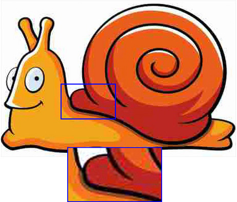
(a) Corrupted

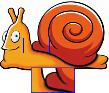
(b) DIP (2400 iterations)

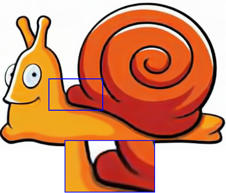
(c) OSC

Figure 2: Blind restoration of a JPEG-compressed image

Figure 3 shows the denoising results of DIP and OSC, where (c) is selected by PSNR, (d) is the result of suggested iteration which is selected based on human inspection, (e) the result of OSC. The result of OSC is close to the PSNR-maximum image, and better than the suggested iteration.

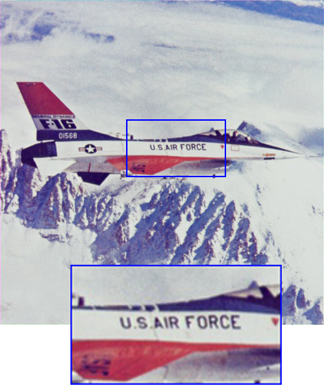
(a) GT

(b) Input

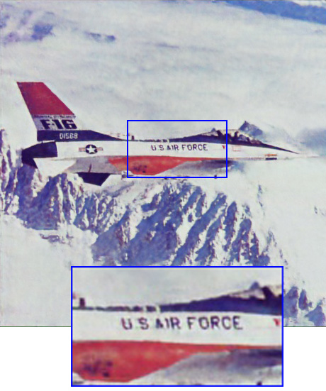
(c) DIP (1804 iterations)

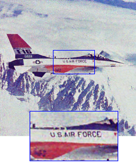
(d) DIP (3000 iterations)

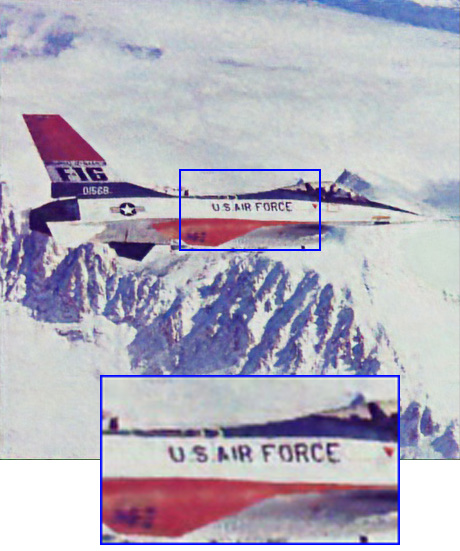
(e) OSC

Figure 3: Blind image denoising

We have done the denoising experiments on Kate, Snail, F16 images and the results are shown in table 1. The JPEG corrupted Snail image has been used as the ground truth. DIP (PSNR) gives out the maximum PSNR and DIP (Iteration) shows the PSNR of 3000 iteration which is the default value in the DIP code. The PSNR values of images selected by OSC are listed in the 4th row followed by the maximum PSNR that we have gotten during OSC iterating. Accuracy is the ratio of 4th row to 5th row. As shown in table 1, OSC results are comparable to DIP which needs the supervision of humans. The Max PSNR is close to DIP (PSNR) which means that the addition of pseudo noise has little influence on the noisy image reconstruction.

Table 1: Denoising results

Image	Kate	Snail	F16
DIP (PSNR)	31.39	27.30	30.82
DIP (Iteration)	31.27	26.7	29.29
OSC	30.73	26.44	29.80
Max PSNR	31.19	27.42	30.33
Accuracy	98.53%	96.43%	98.25%

3.2 Super-resolution

For super-resolution, we train OSC to minimize equation (2) using $E(x;x_{0}+pn)=\|d(x)-(x_{0}+d(pn))\|^{2}$ where $x$ is the reconstructed image, $x_{0}$ a down-sampled observation, $d(.)$ is Lanczos down sample method which is used by [12]. We tested DIP and OSC on Set5 [1] and Set14 [15] with down scales 4 and/or 8.

Figure 4 has shown the examples of 4x image super-resolution, where (c) is stopped at the PSNR-maximum point, (d) is stopped at the suggested 2000 iteration, (c) is generated by OSC. OSC results are very close to the PSNR-maximum version of DIP, which means that OSC has found the near-optimal solution for super-resolution inverse problem automatically.

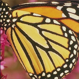
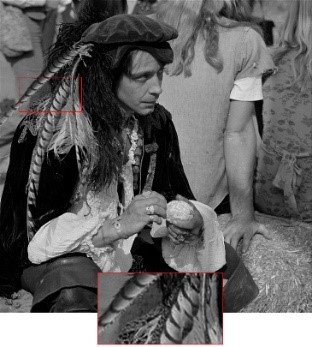
(a) Original Image

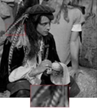
(b) Bicubic

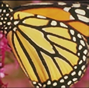
(c) DIP (Max PSNR)

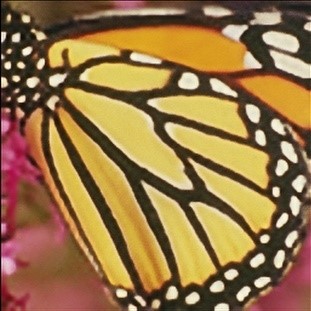
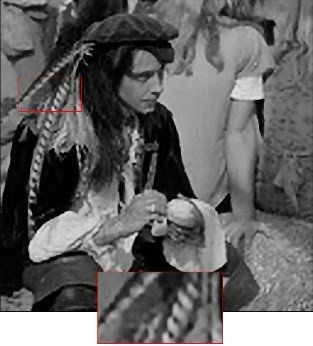
(d) DIP (2000 Iterations)

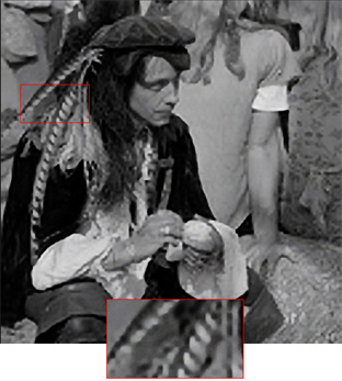
(e) OSC

Figure 4: 4x image super-resolution

Table 2 shows the 4x super-resolution results of Set5 where maximum PSNRs of DIP are in the 1st row, PSNRs of 2000 iterations DIP are in the 2nd row, OSC results are in the 3rd row followed by maximum PSNRs of OSC and accuracy in the last. Similarly, the results of 4x and 8x super-resolution on Set14 are shown in table 3 and table 4. DIP was stopped at 8000 iterations in the 8x super-resolution experiment. From table 2, table 3 and table 4, we believe that OSC is very good at finding optimal stopping iteration for super-resolution problems because the accuracy is higher than 95% for all testing images.

Table 2: 4x super-resolution on Set5

Image	Baby	Bird	Butterfly	Head	Woman
DIP (PSNR)	30.66	30.33	24.93	28.90	27.50
DIP (Iteration)	29.78	29.63	24.69	28.42	26.93
OSC	30.43	29.47	24.41	28.05	26.14
Max PSNR	30.75	29.83	24.67	28.71	27.32
Accuracy	98.96%	98.79%	98.95%	97.70%	95.68%

Table 3: 4x super-resolution on Set14

Image	Baboon	Barbara	Bridge	Coastguard	Comic	Face	Flowers	Foreman	Lenna	Man	Monarch	Pepper	Ppt3	Zebra
DIP (PSNR)	20.45	23.95	23.25	24.56	21.00	29.00	25.04	28.29	29.56	25.19	29.48	28.50	22.99	24.49
DIP (Iteration)	20.27	23.78	23.13	24.39	20.86	28.38	24.48	27.83	29.03	24.81	28.74	27.87	22.67	24.07
OSC	20.36	22.75	23.22	24.31	20.37	28.74	23.11	27.46	28.32	24.32	29.12	28.31	22.88	24.09
Max PSNR	20.37	23.89	23.25	24.34	20.98	28.82	24.85	27.65	29.23	25.12	29.28	28.40	23.23	24.28
Accuracy	99.95%	95.23%	99.87%	99.88%	97.09%	99.72%	93.00%	99.31%	96.89%	96.82%	99.45%	99.68%	98.49%	99.22%

Table 4: 8x super-resolution on Set14

Image	Baboon	Barbara	Bridge	Coastguard	Comic	Face	Flowers	Foreman	Lenna	Man	Monarch	Pepper	Ppt3	Zebra
DIP (PSNR)	19.38	22.35	21.13	22.60	18.42	27.29	21.36	24.08	26.68	22.55	23.96	25.96	18.78	19.62
DIP (Iteration)	19.36	22.33	21.10	22.58	18.37	27.10	21.34	23.89	26.59	22.52	23.92	25.86	18.67	19.58
OSC	19.05	21.46	20.95	22.38	18.03	25.63	20.99	23.08	25.67	21.41	23.72	24.98	18.69	18.85
Max PSNR	19.36	22.34	21.07	22.66	18.39	27.18	21.39	23.80	26.57	22.47	23.92	25.93	18.76	19.62
Accuracy	98.40%	96.06%	99.43%	98.76%	98.04%	94.30%	98.13%	96.97%	96.61%	95.28%	99.16%	96.34%	99.63%	96.08%

3.3 Inpainting

For inpainting, we train OSC to minimize equation (2) using $E(x;x_{0}+pn)=\|(x-(x_{0}+pn))\odot m\|^{2}$ where $x$ is the reconstructed image, $x_{0}$ is a corrupted observation, $\odot$ is Hadamard’s product, $m\in\{0,1\}^{F\times W}$ is a binary mask of the missing pixels in $x_{0}$, $F$ is the height and $W$ is the width of the image. $pn$ is the pseudo noise generated by equation (6), where $a$, $b$, $c$ are channel, row, column index respectively, $A_{b}\in\mathbb{U}(\frac{1}{50},\frac{1}{25})$, $\theta_{b}\in\mathbb{U}(\frac{\pi\times 20}{W},\frac{\pi\times 40}{W})$, $\mathbb{U}$ is the random uniform distribution. The pseudo-noise component is calculated by equation (7), where $L=\sum_{j=1}^{N}m_{j}$, $N$ is the number of elements in the image.

$$pn_{a,b,c} =A_{b}\times\sin(\theta_{b}\times c)$$ (6)

$$e_{i} =\frac{1}{L}\sum_{j=1}^{N}x_{i,j}\times pn_{j}\times m_{j}$$ (7)

Figures 5 and 6 shows the results of regional recovery. Figure 7 shows the results of two inpainting approaches. Table 5 lists PSNRs of the experiments. The OSC results are very close to DIP maximum PSNR which means the OSC method is fully capable of finding optimal stopping iteration automatically.

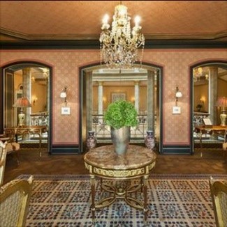
(a) Original Image

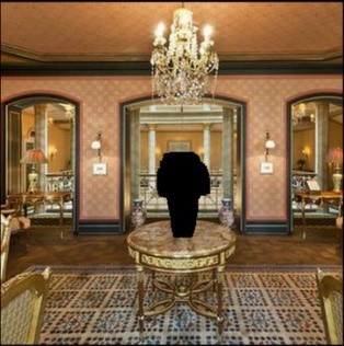
(b) Corrupted Image

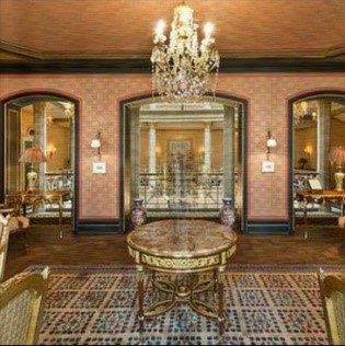
(c) DIP (Max PSNR)

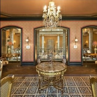
(d) DIP (5000 iterations)

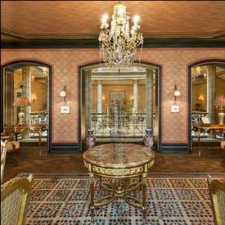
(e) OSC

Figure 5: The recovery of image Vase

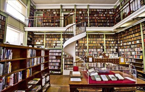
(a) Original Image

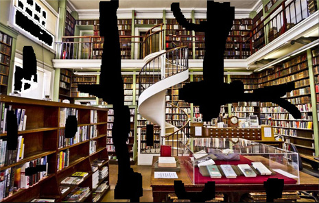
(b) Corrupted Image

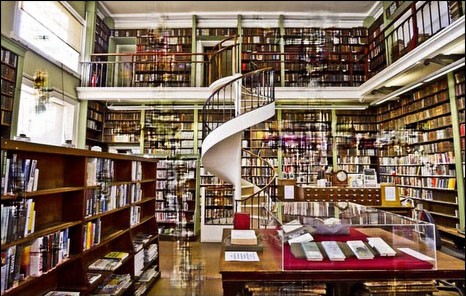
(c) DIP (Max PSNR)

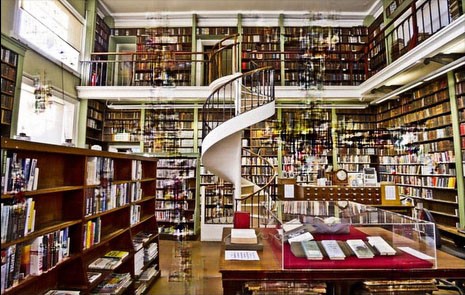
(d) DIP (5000 iterations)

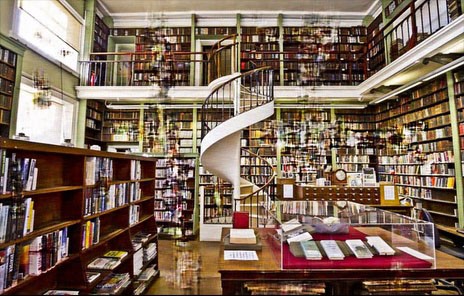
(e) OSC

Figure 6: The recovery of image Library

(a) Original Image

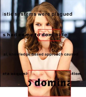
(b) Corrupted Image

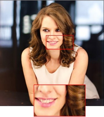
(c) DIP (Max PSNR)

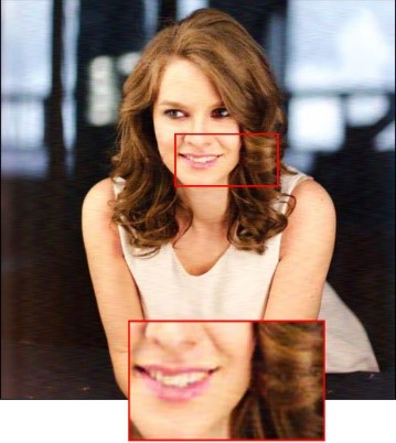
(d) OSC

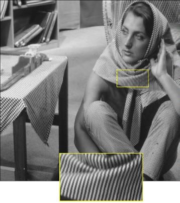
(e) Original Image

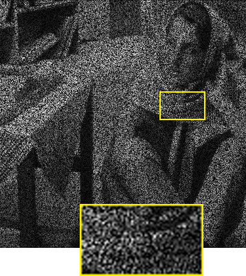
(f) Corrupted Image

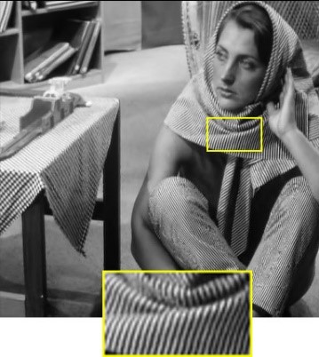
(g) DIP (Max PSNR)

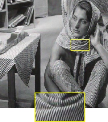
(h) OSC

Figure 7: Two inpainting approaches

Table 5: PSNRs of inpainting experiments

Image	Kate	Library	Vase	Barbara
DIP (PSNR)	40.19	19.22	29.14	31.91
DIP (Iteration)	39.14	19.08	27.76	30.90
OSC	33.74	18.64	28.67	30.97
Max PSNR	35.33	18.72	28.71	31.07
Accuracy	95.50%	99.57%	99.86%	99.68%

4 Conclusion

In this work, we have developed Orthogonal Stopping Criterion (OSC) which can endow Deep Image Prior (DIP) the power of automation. The automatic stopping mechanic is essential to DIP in real-world applications because the Peak Signal to Noise Ratio (PSNR) and human supervision are both unavailable or hard to reach. By adding pseudo noise to the corrupted image, OSC can find the near-optimal result automatically which is very close to the one with maximum PSNR in our experiments. Additionally, the pseudo noise has little influence on the maximum PSNR which has been verified by the experiments. The ratios of OSC PSNR to the maximum are higher than 95% in 38 out of 40 experiments. Many of them are even higher than 99%. Although, the results of DIP are comparable to OSC, they are selected based on PSNR or human inspection. In all, we believe that OSC is an indispensable part of DIP-based single image inverse systems.

References

- [1] Marco Bevilacqua, Aline Roumy, Christine Guillemot, and Marie Line Alberi-Morel. Low-complexity single-image super-resolution based on nonnegative neighbor embedding. 2012.
- [2] Cristóvão Cruz, Alessandro Foi, Vladimir Katkovnik, and Karen Egiazarian. Nonlocality-reinforced convolutional neural networks for image denoising. IEEE Signal Processing Letters, 25(8):1216–1220, 2018.
- [3] Hongyun Gao, Xin Tao, Xiaoyong Shen, and Jiaya Jia. Dynamic scene deblurring with parameter selective sharing and nested skip connections. In Proceedings of the IEEE Conference on Computer Vision and Pattern Recognition, pages 3848–3856, 2019.
- [4] Zheng Hui, Xiumei Wang, and Xinbo Gao. Fast and accurate single image super-resolution via information distillation network. In Proceedings of the IEEE conference on computer vision and pattern recognition, pages 723–731, 2018.
- [5] Stamatios Lefkimmiatis. Universal denoising networks: a novel cnn architecture for image denoising. In Proceedings of the IEEE conference on computer vision and pattern recognition, pages 3204–3213, 2018.
- [6] Ding Liu, Bihan Wen, Yuchen Fan, Chen Change Loy, and Thomas S Huang. Non-local recurrent network for image restoration. In Advances in Neural Information Processing Systems, pages 1673–1682, 2018.
- [7] Gary Mataev, Peyman Milanfar, and Michael Elad. Deepred: Deep image prior powered by red. In Proceedings of the IEEE International Conference on Computer Vision Workshops, pages 0–0, 2019.
- [8] Seong-Jin Park, Hyeongseok Son, Sunghyun Cho, Ki-Sang Hong, and Seungyong Lee. Srfeat: Single image super-resolution with feature discrimination. In Proceedings of the European Conference on Computer Vision (ECCV), pages 439–455, 2018.
- [9] Tobias Plötz and Stefan Roth. Neural nearest neighbors networks. In Advances in Neural Information Processing Systems, pages 1087–1098, 2018.
- [10] Xin Tao, Hongyun Gao, Xiaoyong Shen, Jue Wang, and Jiaya Jia. Scale-recurrent network for deep image deblurring. In Proceedings of the IEEE Conference on Computer Vision and Pattern Recognition, pages 8174–8182, 2018.
- [11] Dmitry Ulyanov, Andrea Vedaldi, and Victor Lempitsky. Deep image prior. In Proceedings of the IEEE Conference on Computer Vision and Pattern Recognition, pages 9446–9454, 2018.
- [12] Dmitry Ulyanov, Andrea Vedaldi, and Victor Lempitsky. Deep image prior. In Submitted to IJCV, pages 1–22, 2018.
- [13] Yifan Wang, Federico Perazzi, Brian McWilliams, Alexander Sorkine-Hornung, Olga Sorkine-Hornung, and Christopher Schroers. A fully progressive approach to single-image super-resolution. In Proceedings of the IEEE Conference on Computer Vision and Pattern Recognition Workshops, pages 864–873, 2018.
- [14] Wenming Yang, Xuechen Zhang, Yapeng Tian, Wei Wang, Jing-Hao Xue, and Qingmin Liao. Deep learning for single image super-resolution: A brief review. IEEE Transactions on Multimedia, 2019.
- [15] Roman Zeyde, Michael Elad, and Matan Protter. On single image scale-up using sparse-representations. In International conference on curves and surfaces, pages 711–730. Springer, 2010.
- [16] Kai Zhang, Wangmeng Zuo, and Lei Zhang. Ffdnet: Toward a fast and flexible solution for cnn-based image denoising. IEEE Transactions on Image Processing, 27(9):4608–4622, 2018.
- [17] Yulun Zhang, Kunpeng Li, Kai Li, Lichen Wang, Bineng Zhong, and Yun Fu. Image super-resolution using very deep residual channel attention networks. In Proceedings of the European Conference on Computer Vision (ECCV), pages 286–301, 2018.