Practical computation of the diffusion MRI signal of realistic neurons based on Laplace eigenfunctions

Abstract

[Abstract]The complex transverse water proton magnetization subject to diffusion-encoding magnetic field gradient pulses in a heterogeneous medium such as brain tissue can be modeled by the Bloch-Torrey partial differential equation. The spatial integral of the solution of this equation in realistic geometry provides a gold-standard reference model for the diffusion MRI signal arising from different tissue micro-structures of interest. A closed form representation of this reference diffusion MRI signal has been derived twenty years ago, called Matrix Formalism that makes explicit the link between the Laplace eigenvalues and eigenfunctions of the biological cell and its diffusion MRI signal. In addition, once the Laplace eigendecomposition has been computed and saved, the diffusion MRI signal can be calculated for arbitrary diffusion-encoding sequences and b-values at negligible additional cost.

Up to now, this representation, though mathematically elegant, has not been often used as a practical model of the diffusion MRI signal, due to the difficulties of calculating the Laplace eigendecomposition in complicated geometries. In this paper, we present a simulation framework that we have implemented inside the MATLAB-based diffusion MRI simulator SpinDoctor that efficiently computes the Matrix Formalism representation for realistic neurons using the finite elements method. We show the Matrix Formalism representation requires around a few hundred eigenmodes to match the reference signal computed by solving the Bloch-Torrey equation when the cell geometry comes from realistic neurons. As expected, the number of required eigenmodes to match the reference signal increases with smaller diffusion time and higher b-values. We also converted the eigenvalues to a length scale and illustrated the link between the length scale and the oscillation frequency of the eigenmode in the cell geometry. We gave the transformation that links the Laplace eigenfunctions to the eigenfunctions of the Bloch-Torrey operator and computed the Bloch-Torrey eigenfunctions and eigenvalues. This work is another step in bringing advanced mathematical tools and numerical method development to the simulation and modeling of diffusion MRI.

Diffusion MRI is an imaging modality that can be used to probe the tissue micro-structure by encoding the incoherent motion of water molecules with magnetic field gradient pulses. Incoherent motion during the diffusion-encoding time causes a signal attenuation from which the apparent diffusion coefficient (ADC), and possibly higher order diffusion terms, can be calculated ^{1, 2, 3}. For free diffusion, the root of the mean squared displacement of molecules is given by $\bar{x}=\sqrt{2\,dim\,\mathcal{D}_{0}t}$, where $dim$ is the spatial dimension, $\mathcal{D}_{0}$ is the intrinsic diffusion coefficient, and $t$ is the diffusion time. In biological tissue, diffusion is usually hindered or restricted (for example, by cell membranes) and the mean square displacement is smaller than in the case of free diffusion. This deviation from free diffusion can be used to infer information about the tissue micro-structure.

Using diffusion MRI to get tissue structural information in the brain has been the focus of much experimental and modeling work in recent years ^{4, 5, 6, 7, 8, 9, 10, 11, 12, 13, 14, 15, 16, 17, 18, 19}. In terms of modeling, the predominant approach up to now has been adding the contributions to the diffusion MRI signal from simple geometrical components and extracting model parameters of interest. Numerous biophysical models subdivide the tissue into compartments described by spheres, ellipsoids, cylinders, and the extra-cellular space ^{12, 13, 14, 16, 20, 21, 22, 17, 23, 24}. Some model parameters of interest include axon diameter and orientation, neurite density, dendrite structure, the volume fraction and size distribution of cylinder and sphere components and the effective diffusion coefficient or tensor of the extra-cellular space. The need for a mathematically rigorous model of the diffusion MRI signal arising from realistic cellular structures was re-iterated in recent review papers ^{25, 26, 27}.

There is a gold-standard reference model of the diffusion MRI signal, it is the Bloch-Torrey partial differential equation (PDE) that describes the time evolution of the complex transverse water proton magnetization subject to diffusion-encoding magnetic field gradient pulses. For this model to be the gold-standard, we mean of course that it should be posed in realistic tissue and cell geometries. This PDE can be posed in a heterogeneous medium containing different cell structures and the extra-cellular space. The spatial integral of the solution of the PDE provides a reference model for the diffusion MRI signal arising from different tissue micro-structures of interest. Because of the high computational cost of solving the Bloch-Torrey equation in complicated cell geometries, this gold standard model has been used primarily as a "forward model" or "simulation framework", in which one changes the inputs parameters such as cell geometry, intrinsic diffusion coefficient, membrane permeability, and study the resulting changes to the MRI signal. This is in contrast to "inverse models", which are used to robustly estimate the model parameters of interest from the MRI signal, the idea being that the "inverse models" have been formulated in such a way so that the model parameters can be correlated to biological information in the imaging voxel. "Inverse models" include the biophysical models cited above. Nevertheless, given the recent availability of vastly powerful computational resources and computer memory, it is possible that simulation frameworks may become directly useful for parameter estimation in the future (for some recent works in this direction, see ^{18, 28}).

Two main groups of simulation frameworks for diffusion MRI are 1) using random walkers to mimic the diffusion process in a geometrical configuration; 2) solving the Bloch-Torrey partial differential equation using the finite elements method (FEM). The first group is referred to as Monte-Carlo simulations in the literature and previous works include ^{29, 30, 31, 18, 32}. A GPU-based acceleration of Monte-Carlo simulation was proposed in ^{33, 34}. Some software packages using this approach include

1. Camino Diffusion MRI Toolkit³¹, developed at UCL (http://cmic.cs.ucl.ac.uk/camino/);

2. DIFSIM³², developed at UC San Diego (http://csci.ucsd.edu/projects/simulation.html);

3. Diffusion Microscopist Simulator³⁰, developed at Neurospin, CEA;

4. We mention also that the GPU-based Monte-Carlo simulation code described in ³³ is available upon request from the authors.

Many works^{35, 36, 37, 38, 39, 40, 18, 28} on model formulation and validation for brain tissue diffusion MRI used Monte-Carlo simulations. The second group of simulations, which up to now has been less often used by the diffusion MRI community, relies on solving the Bloch-Torrey equation in a geometrical configuration using the finite elements method (FEM) ^{41, 42, 43, 44, 45}(an alternative to the FEM is the finite difference method⁴⁶). Some of the recent works about FEM diffusion MRI simulations focused on improving its computational efficiency, by using high-performance computing ^{47, 48} for large-scale simulations on supercomputers, by discretization on manifolds for thin-layer and thin-tube media ⁴⁹, by integrating with Cloud computing resources ⁵⁰. Our previous works in neuron diffusion MRI simulations with FEM include the simulation of neuronal dendrites using a tree model ⁵¹ and the demonstration that diffusion MRI signals reflect the cellular organization of cortical gray matter, these signals being sensitive to cell size and the presence of large neurons such as the spindle (von Economo) neurons ^{52, 53}.

In one recent paper⁵⁴, we presented SpinDoctor, a MATLAB-based diffusion MRI simulation toolbox that solves the Bloch-Torrey PDE using FEM and an adaptive time stepping method. SpinDoctor provides a user-friendly interface to easily define cell configurations relevant to the brain white matter. Though the original version of SpinDoctor focused on the brain white matter, we also performed simulations of the diffusion MRI signal from a dendrite branch to compare the computational efficiency of SpinDoctor with the Monte-Carlo based simulations of Camino (http://cmic.cs.ucl.ac.uk/camino/). It was shown that at equivalent accuracy, SpinDoctor simulations of the extra-cellular space in the brain white matter is 100 times faster than Camino and SpinDoctor simulations of a neuronal dendrite tree is 400 times faster than Camino. We refer the reader to ⁵⁴ for detailed numerical validation of SpinDoctor simulations and timing comparisons with Camino.

In another recent paper⁵⁵, we presented a module of SpinDoctor called the Neuron Module that enables diffusion MRI simulations for a group of 36 pyramidal neurons and a group of 29 spindle neurons whose morphological descriptions were found in the neuron repository NeuroMorpho.Org ⁵⁶. The key to making accurate simulation possible is the use of high quality finite elements meshes for the neurons. For this, we corrected and improved the quality of the geometrical descriptions of the neurons, the details of which can be found in ⁵⁵. After processing, we produced high quality finite elements meshes for the 65 neurons. These finite elements meshes range from having 15163 nodes to 622553 nodes. Currently, the simulations in the Neuron Module enforce homogeneous Neumann boundary conditions, meaning the spin exchange across the cell membrane is assumed to be negligible. In ⁵⁵ we performed an accuracy and computational timing study of the serial SpinDoctor finite elements simulation and a GPU implementation of the Monte-Carlo simulation³³. We showed that at equivalent accuracy, if only one gradient direction needs to be simulated, SpinDoctor is faster than GPU Monte-Carlo. Because the GPU Monte-Carlo method is inherently parallel, if many gradient directions need to be simulated, there is a break-even point when GPU Monte-Carlo becomes faster than SpinDoctor. In particular, at equivalent accuracy, we showed the ratio between the GPU Monte-Carlo computational time and the SpinDoctor computational time for 1 gradient direction ranges from 31 to 72 for the whole neuron simulations.

In this paper, we present a new module of SpinDoctor called the Matrix Formalism Module. Taking the Bloch-Torrey equation as the gold-standard reference model, a closed form representation of the reference signal has been derived twenty years ago, that is based on the eigenvalues and eigenfunctions of the Laplace operator in the relevant cell geometry. This representation frequently goes under the name of Matrix Formalism. The version that uses the impulse approximation of the diffusion-encoding sequence is first found in ⁵⁷ and the version that uses the piecewise constant approximation of the diffusion-encoding sequence is first found in ⁵⁸. There have been numerous works using Matrix Formalism in elementary geometries such as the line segment, the disk, and the sphere, as well as geometries which can be written as tensor products of these elementary geometries. We cite ^{59, 60, 61} and refer the reader to the literature surveys on the Matrix Formalism contained in those articles.

There are two advantages to the Matrix Formalism signal representation. First, the analytical advantage is that this representation makes explicit the link between the Laplace eigenvalues and eigenfunctions of the biological cell and its diffusion MRI signal. This clear link may help in the formulation of reduced models of the diffusion MRI signal that is closer to the physics of the problem. Second, the computational advantage is that once the Laplace eigendecomposition has been computed and saved, the diffusion MRI signal can be calculated for arbitrary diffusion-encoding sequences and b-values at negligible additional cost. This will make it possible to use the Matrix Formalism as the inner loop of optimization procedures.

Up to now, Matrix Formalism, as a closed form signal representation, though mathematically elegant, has not been often used as a practical way of computing the diffusion MRI signal in complicated geometries such as realistic neurons. The calculation of the Laplace eigendecomposition in realistic neurons using Monte-Carlo based simulations would be essentially impossible due to computational time and memory limitations. Using the FEM, the eigenfunctions of the Laplace operator can be numerically computed in an efficient way and this is the approach we will describe in what follows.

1 Theory

Consider a domain $\Omega$ that describes the geometry of a neuron. In this paper, we neglect the effect of water exchange between the neuron and the extra-cellular space. Thus, impermeable boundary conditions are imposed on $\Omega$.

1.1 Bloch-Torrey PDE

In diffusion MRI, a time-varying magnetic field gradient is applied to the tissue to encode water diffusion. Denoting the effective time profile of the diffusion-encoding magnetic field gradient by $f(t)$, and let the vector ${\bm{g}}$ contain the amplitude and direction information of the magnetic field gradient, the complex transverse water proton magnetization in the rotating frame satisfies the Bloch-Torrey PDE:

$$\begin{split}\frac{\partial}{\partial t}{M({\bm{x}},t)}=&-{\mathbb{i}}\gamma f(t){\bm{g}}\cdot{\bm{x}}\,M({\bm{x}},t)+\nabla\cdot(\mathcal{D}_{0}\nabla M({\bm{x}},t)),\quad{\bm{x}}\in\Omega,\end{split}$$ (1)

where $\gamma=2.67513\times 10^{8}\,\rm rad\,s^{-1}T^{-1}$ is the gyromagnetic ratio of the water proton, ${\mathbb{i}}$ is the imaginary unit, $\mathcal{D}_{0}$ is the intrinsic diffusion coefficient in the compartment $\Omega$. Neglecting water exchange between the neuron and the extra-cellular space, the boundary condition on the boundary $\Gamma=\partial\Omega$ is the homogeneous Neumann condition:

$$\mathcal{D}_{0}\nabla M({\bm{x}},t)\cdot{\bm{n}}=0,\quad{\bm{x}}\in\Gamma,$$ (2)

where ${\bm{n}}$ is the unit outward pointing normal vector. The PDE also needs initial conditions: $M({\bm{x}},0)=\rho$, where $\rho$ is the initial spin density. The magnetization is a function of position ${\bm{x}}$ and time $t$, and depends on the diffusion gradient vector ${\bm{g}}$ and the time profile $f(t)$. The Bloch-Torrey PDE is a well accepted reference model for the diffusion MRI signal by the diffusion MRI research community.

For simplicity, we only show results for one type of diffusion-encoding sequences in this paper: the pulsed-gradient spin echo (PGSE) ² sequence. It contains two rectangular pulses of duration $\delta$, separated by a time interval $\Delta-\delta$, for which the effective profile $f(t)$ is

$$f(t)=\begin{cases}1,\quad&t_{1}\leq t\leq t_{1}+\delta,\\ -1,\quad&t_{1}+\Delta<t\leq t_{1}+\Delta+\delta,\\ 0,\quad&\text{otherwise,}\end{cases}$$ (3)

where $t_{1}$ is the starting time of the first gradient pulse with $t_{1}+\Delta>T_{E}/2$, $T_{E}$ is the echo time at which the signal is measured. The diffusion MRI signal due to spins in the domain $\Omega$ is the space integral of $M({\bm{x}},T_{E})$ in $\Omega$:

$$S^{\text{BTPDE}}:=\int_{{\bm{x}}\in\Omega}M({\bm{x}},T_{E})\;d{\bm{x}}.$$ (4)

In a diffusion MRI experiment, the pulse sequence (time profile $f(t)$) is usually fixed, while ${\bm{g}}$ is varied in amplitude (and possibly also in direction). The signal $S$ is usually plotted against a quantity called the $b$-value. The $b$-value depends on ${\bm{g}}$ and $f(t)$ and is defined as

$$b({\bm{g}},f)=\gamma^{2}\|{\bm{g}}\|^{2}\int_{0}^{T_{E}}du\left(\int_{0}^{u}f(s)ds\right)^{2}.$$

The reason for these definitions is that in a homogeneous medium, the signal attenuation is $e^{-\mathcal{D}_{0}b}$.

An important quantity that can be derived from the diffusion MRI signal is the “Apparent Diffusion Coefficient” (ADC), defined as (assume time profile $f$ is fixed):

$$ADC:=\left.-\frac{\partial}{\partial b}\log{\frac{S(b)}{S(0)}}\right|_{b=0}.$$ (5)

The ADC gives an indication of the root mean squared distance travelled by water molecules in the gradient direction ${\bm{u_{g}}}={\bm{g}}/\|{\bm{g}}\|$, averaged over all starting positions.

1.2 Matrix Formalism signal representation

It is known that using the Matrix Formalism ^{57, 58}, the diffusion MRI signal has the following representation for the PGSE sequence. Let $\phi_{n}({\bm{x}})$ and $\lambda_{n}$, $n=1,\cdots$, be the $L^{2}$-normalized eigenfunctions and eigenvalues associated to the Laplace operator with homogeneous Neumann boundary conditions (the surface of the neurons are supposed impermeable):

$$-\nabla\mathcal{D}_{0}\left(\nabla\phi_{n}({\bm{x}})\right) =\lambda_{n}\phi_{n}({\bm{x}}), \quad{\bm{x}}\in\Omega,$$

$$\mathcal{D}_{0}\nabla\phi_{n}({\bm{x}})\cdot{\bm{\nu}}({\bm{x}}) =0, \quad{\bm{x}}\in\Gamma.$$

We assume the non-negative real-valued eigenvalues are ordered in non-decreasing order:

$$0=\lambda_{1}<\lambda_{2}\leq\lambda_{3}\leq\cdots$$

so that $\lambda_{1}=0$ (this means the first Laplace eigenfunction is the constant function). There is only one constant eigenfunction because we assume the neuron is a connected domain. Let $L$ be the diagonal matrix containing the first $N_{eig}$ Laplace eigenvalues:

$$L=\text{diag}[\lambda_{1},\lambda_{2},\cdots,\lambda_{N_{eig}}]\in\mathbb{R}^{N_{eig}\times N_{eig}}.$$ (6)

Let $W({\bm{g}})$ be the ${N_{eig}\times N_{eig}}$ matrix whose entries are:

$$W({\bm{g}})=g_{x}A^{x}+g_{y}A^{y}+g_{z}A^{z}$$ (7)

where ${\bm{g}}=(g_{x},g_{y},g_{z}),$ and

$$A^{i}=\begin{bmatrix}a_{mn}^{i}\end{bmatrix},\quad i=\{x,y,z\},\quad 1\leq m,n\leq N_{eig},$$ (8)

are three symmetric ${N_{eig}\times N_{eig}}$ matrices whose entries are the first order moments in the coordinate directions of the product of pairs of eigenfunctions:

$$\begin{split}a_{mn}^{x}&=\int_{\Omega}x\phi_{m}({\bm{x}})\phi_{n}({\bm{x}})d{\bm{x}},\;\\ a_{mn}^{y}&=\int_{\Omega}y\phi_{m}({\bm{x}})\phi_{n}({\bm{x}})d{\bm{x}},\\ a_{mn}^{z}&=\int_{\Omega}z\phi_{m}({\bm{x}})\phi_{n}({\bm{x}})d{\bm{x}}.\end{split}$$

We define the complex-valued matrix $K({\bm{g}})$:

$$K({\bm{g}})\equiv L+{\mathbb{i}}\gamma W({\bm{g}}).$$ (9)

Then the following matrix

$$H({\bm{g}},f)=e^{-K\delta}e^{-L(\Delta-\delta)}e^{-K^{*}\delta},$$ (10)

gives the Matrix Formalism representation of the solution to the Bloch-Torrey PDE. For a constant initial density, the Matrix Formalism signal representation is the entry in the first row and first column of $H({\bm{g}},f)$, multiplied by $S_{0}$, the signal with zero b-weighting:

$$S^{\text{MF}}({\bm{g}},f)=\rho|\Omega|H_{11}({\bm{g}},f)=S_{0}H_{11}({\bm{g}},f).$$ (11)

We note that in Eq. 10 the matrix $L$ in the exponent is diagonal and in this case, the matrix exponential is also diagonal. The notation ^∗ denotes the matrix complex conjugate transpose. In order to calculate the non-diagonal matrix exponentials $e^{-K\delta}$ and $e^{-K^{*}\delta}$, we diagonalize the matrix $K({\bm{g}})$

$$K({\bm{g}})=V\Sigma V^{-1},$$ (12)

where $V$ has the eigenvectors in the columns and $\Sigma$ has the eigenvalues on the diagonal. Then $e^{-K\delta}=Ve^{-\delta\Sigma}V^{-1}$ and $e^{-K^{*}\delta}=\left(V^{-1}\right)^{*}e^{-\delta\Sigma^{*}}V^{*}$; hence, $H({\bm{g}},f)$ can be written as

$$H({\bm{g}},f)=Ve^{-\delta\Sigma}V^{-1}e^{-(\Delta-\delta)L}\left(V^{-1}\right)^{*}e^{-\delta\Sigma^{*}}V^{*}.$$ (13)

For a derivation of the Matrix Formalism formula, see Appendix A. For the transformation between the Laplace eigenfunctions and the eigenfunctions of the Bloch-Torrey operator, see Appendix B.

From the Matrix Formalism signal, the analytical expression for its ADC is the following (for a derivation, see ⁶²):

$$\frac{ADC}{\mathcal{D}_{0}}=\sum_{n=1}^{N_{eig}}\frac{({\bm{u_{g}}}\cdot{\bm{a}}_{1n})^{2}\lambda_{n}\int_{0}^{T_{E}}F(t)\left(\int_{0}^{t}e^{-\lambda_{n}(t-s)}f(s)ds\right)dt}{\mathcal{D}_{0}\int_{0}^{T_{E}}F^{2}(t)dt},$$

where $F(t)\equiv\int_{0}^{t}f(s)ds$ and the coefficients ${\bm{a}}_{1n}=\begin{bmatrix}a_{1n}^{x},a_{1n}^{y},a_{1n}^{z}\end{bmatrix}^{T}$ are

$$\begin{split}a_{1n}^{x}&=\frac{1}{\sqrt{|\Omega|}}\int_{\Omega}x\phi_{n}({\bm{x}})d{\bm{x}},\;\\ a_{1n}^{y}&=\frac{1}{\sqrt{|\Omega|}}\int_{\Omega}y\phi_{n}({\bm{x}})d{\bm{x}},\;\\ a_{1n}^{z}&=\frac{1}{\sqrt{|\Omega|}}\int_{\Omega}z\phi_{n}({\bm{x}})d{\bm{x}}.\end{split}$$ (14)

We remind the reader that the first Laplace eigenfunction is the constant function.

To clarify the relationship between the ADC and the diffusion encoding direction ${\bm{u_{g}}}$, we rewrite the Matrix Formalism ADC as:

$$\frac{ADC({\bm{u_{g}}},f)}{\mathcal{D}_{0}}={\bm{u_{g}}}^{T}\frac{D^{\text{MF}}(f)}{\mathcal{D}_{0}}{\bm{u_{g}}},$$ (15)

where the Matrix Formalism effective diffusion tensor is seen to be:

$$\frac{D^{\text{MF}}(f)}{\mathcal{D}_{0}}=\sum_{n=1}^{N_{eig}}J(\lambda_{n},f){\bm{a}}_{1n}{\bm{a}}_{1n}^{T},$$ (16)

with $J(\lambda_{n},f)$ depending on $\lambda_{n}$ and $f$:

$$J(\lambda_{n},f)=\frac{\lambda_{n}\int_{0}^{T_{E}}F(t)\left(\int_{0}^{t}e^{-\lambda_{n}(t-s)}f(s)ds\right)dt}{\mathcal{D}_{0}\int_{0}^{T_{E}}F^{2}(t)dt}.$$ (17)

We also allow the possibility of computing the Matrix Formalism Gaussian Approximation (MFGA) signal, given as

$$S^{\text{MFGA}}({\bm{g}},f)=\rho|\Omega|\exp\left(-{\bm{u_{g}}}^{T}D^{\text{MF}}(f){\bm{u_{g}}}\;b\right).$$ (18)

2 Method

In a recent work, we have taken the morphological reconstructions of some realistic neurons from NeuroMorpho.Org ⁶³ and processed them to create high quality finite elements meshes. The procedure is described in ⁵⁵. Specifically, there are 65 realistic neurons whose finite elements meshes we have made available to the public, with the mesh size ranges from having 15163 nodes to 622553 nodes. These are the finite elements meshes we use in the procedure described below to calculate the Matrix Formalism signal. To be clear, each neuron finite elements mesh consists of

1. a list of $N_{v}$ nodes in three dimensions;

2. a list of $N_{e}$ tetrahedral elements ($4\times N_{e}$ indices referencing the nodes);

2.1 Finite elements discretization of the Laplace operator

In SpinDoctor, the finite elements space is the space of continuous piecewise linear functions on tetrahedral elements in three dimensions (known as $P_{1}$). This space has a set of basis functions whose number is exactly the number of finite elements nodes:

$$\{\varphi_{k}({\bm{x}})\},\quad k=1,\dots,N_{v}.$$

Let the finite elements nodes be denoted $\bm{q}_{1},\cdots,\bm{q}_{N_{v}}$. The basis function $\varphi_{k}({\bm{x}})$ is a piece-wise linear function, non-zero on the tetrahedra that touch the node $\bm{q}_{k}$, and zero on all other tetrahedra. On a tetrahedron that touches $\bm{q}_{k}$, $\varphi_{k}({\bm{x}})$ is equal to $1$ on $\bm{q}_{k}$ and it is equal to $0$ on the other 3 vertices of the tetrahedron. This completely describes the piece-wise linear function.

Any function in the finite elements space can be written as a linear combination of the above basis functions

$$\sum_{k=1}^{N_{v}}c_{k}\varphi_{k}({\bm{x}}).$$

To discretize the Laplace operator with zero Neumann boundary conditions, two matrices are needed: $\bm{M}\in\mathbb{R}^{N_{v}\times N_{v}}$ and $\bm{S}\in\mathbb{R}^{N_{v}\times N_{v}}$, known in the FEM literature as the mass and stiffness matrices, respectively, which are defined as follows:

$$\bm{M}_{jk}=\int_{\Omega}\varphi_{k}({\bm{x}})\varphi_{j}({\bm{x}})\,d{\bm{x}},\qquad\qquad\bm{S}_{jk}=\int_{\Omega}\mathcal{D}_{0}\,\nabla\varphi_{k}({\bm{x}})\cdot\nabla\varphi_{j}({\bm{x}})\,d{\bm{x}},\quad 1\leq j,k\leq N_{v}.$$

In SpinDoctor, these matrices are assembled from local element matrices and the assembly process is based on vectorized routines of ⁶⁴, which replace expensive loops over elements by operations with 3-dimensional arrays. All local elements matrices in the assembly of $\bm{S}$ and $\bm{M}$ are evaluated at once and stored in a full matrix of size $4\times 4\times N_{e}$, where $N_{e}$ denotes the number of tetrahedral elements.

The finite elements discretization described above changes the continuous Laplace operator eigenvalue problem to the following discrete matrix eigenvalue problem:

$$\begin{split}\text{find }\{\lambda_{n},p_{n}\},\;1\leq n\leq N_{v},\;\text{ such that}\\ \lambda_{n}\bm{M}p_{n}=-\bm{S}p_{n},\;p_{n}\in\mathbb{R}^{N_{v}},\end{split}$$ (19)

where $p_{n}$ is the eigenvector (of $N_{v}$ entries) associated to the eigenvalue $\lambda_{n}$. Moving back to the space of functions (the function space $P_{1}$), the eigenfunction $\phi_{n}({\bm{x}})$ associated to the eigenvalue $\lambda_{n}$ is then

$$\phi_{n}({\bm{x}})=\sum_{j=1}^{N_{v}}p_{n}^{j}\varphi_{j}({\bm{x}}),$$

where the entries of the eigenvector $p_{n}$ are the coefficients of the finite elements basis functions. To obtain the Matrix Formalism signal representation, we calculated the first moments in the three coordinate directions of the product of pairs of eigenfunctions. They can be written in the following form, that involves the first moments of the finite elements basis function pairs, shown in parentheses:

$$\begin{split}a_{mn}^{x}&=\sum_{j=1}^{N_{v}}\sum_{k=1}^{N_{v}}p_{n}^{j}p_{m}^{k}\left(\int_{\Omega}x\;\varphi_{j}({\bm{x}})\varphi_{k}({\bm{x}})d{\bm{x}}\right),\\ a_{mn}^{y}&=\sum_{j=1}^{N_{v}}\sum_{k=1}^{N_{v}}p_{n}^{j}p_{m}^{k}\left(\int_{\Omega}y\;\varphi_{j}({\bm{x}})\varphi_{k}({\bm{x}})d{\bm{x}}\right),\\ a_{mn}^{z}&=\sum_{j=1}^{N_{v}}\sum_{k=1}^{N_{v}}p_{n}^{j}p_{m}^{k}\left(\int_{\Omega}z\;\varphi_{j}({\bm{x}})\varphi_{k}({\bm{x}})d{\bm{x}}\right).\end{split}\quad 1\leq m,n\leq N_{eig}.$$ (20)

2.2 Eigenfunction length scale

The analytical eigenvalues of a line segment of length $H$ are

$$\lambda_{\{1,2,\cdots\}} =\{0,\gamma_{l}\},\gamma_{l}=\mathcal{D}_{0}\left(\frac{\pi}{H/k}\right)^{2},k=1,2,\cdots$$ (21)

To make the link between the computed eigenvalue and the spatial scale of the eigenmode, we will convert the computed $\lambda_{n}$ into a length scale (from the line segment eigenvalue formula):

$$l_{s}(\lambda)=\frac{\pi}{\sqrt{\lambda/\mathcal{D}_{0}}},$$ (22)

and characterize the computed eigenmode by ${l_{s}}(\lambda_{n})$ instead of $\lambda_{n}$. To characterize the directional contribution of the eigenmode we use the fact that its contribution to the ADC in the direction ${\bm{u_{g}}}$ is $J(\lambda_{n},f)({\bm{u_{g}}}\cdot{\bm{a}}_{1n})^{2}$. Thus, we call ${\bm{a}}_{1n}=\begin{bmatrix}a_{1n}^{x},a_{1n}^{y},a_{1n}^{z}\end{bmatrix}^{T}$ the "diffusion direction" of the $n$th eigenmode. We remind that the three components of ${\bm{a}}_{1n}$ are the first moments in the 3 principle axes directions of the associated eigenfunction.

2.3 Eigenvalues interval and minimum length scale

We do not want to compute the entire set of eigenvalues and eigenvectors $\{\lambda_{n},p_{n}\},\ 1\leq n\leq N_{v},$ of the matrix eigenvalue problem in Eq. 19, because the size of $\bm{M}$ and $\bm{S}$ is determined by the finite elements discretization (it is equal to $N_{v}$, the number of finite elements nodes). We remind that for the 65 realistic neurons whose finite elements meshes are available in the Neuron Module of SpinDoctor, the mesh size ranges from having 15163 nodes to 622553 nodes. This means most of the rapidly oscillating eigenmodes in the matrix eigenvalue problem are linked to the finite elements discretization, and not the physics of the problem. To link with the physics of the diffusion in the cell geometry, we set a restricted interval in which to compute the eigenvalues. We set the interval to be $[0,(\pi/l_{s}^{min})^{2}\mathcal{D}_{0}]$, where $l_{s}^{min}$ is the shortest length scale of interest in the cell geometry. In this way, the number of computed eigenmodes, $N_{eig}$, will be much smaller than $N_{v}$.

This restricted eigenvalue interval for the matrix eigenvalue problem was implemented by called the "pdeeig" function in the MATLAB PDE Toolbox, after defining a PDE model whose PDE is the Laplace equation with the diffusion coefficient $\mathcal{D}_{0}$.

3 Results

All the numerical results in this Section concern two neurons:

1. the pyramidal neuron 02b_pyramidal1aACC, whose bounding box is $[-70,113]\mu\text{m}\times[-197,165]\mu\text{m}\times[-14,18]\mu\text{m}$. The geometry is shown in Figure 3. The finite elements mesh of this neuron has 44908 nodes and 171017 tetrahedral elements.

2. the spindle neuron 03b_spindle4aACC, whose bounding box is $[-236,102]\mu\text{m}\times[-65,68]\mu\text{m}\times[-49,6]\mu\text{m}$. The geometry is shown in Figure 4. Two finite elements meshes of this neuron were generated. The fine mesh has 44201 nodes and 160205 elements, the coarser mesh has 17370 nodes and 56163 elements.

The numerical solution of the Bloch-Torrey PDE was computed using SpinDoctor to obtain the reference diffusion MRI signals. The Bloch-Torrey PDE was discretized using P1 finite elements and solved with build-in MATLAB routines for ordinary differential equation (ODE) systems. The time discretization is controlled by setting the absolute and relative tolerances of the ODE solver. We refer the reader to ⁵⁴ for details on how to use SpinDoctor and to ⁵⁵ for simulation parameters for these neuron finite elements meshes.

3.1 Comparing the Matrix Formalism signal with the reference signal

The Matrix Formalism Module computes $S^{\text{MF}}$ in Eq. 11 for the requested b-values and diffusion-encoding sequences. In the simulations below, $\mathcal{D}_{0}=2\times 10^{-3}\,\text{mm}^{2}/\text{s}$. The tolerances of the ODE solution of the finite elements matrix system is set to $atol=10^{-4}$ (absolute tolerance) and $rtol=10^{-2}$ (relative tolerance). We simulated two diffusion-encoding sequences: SEQ1 (PGSE, $\delta=10.6\text{ms},\Delta=13\text{ms}$); SEQ2 (PGSE, $\delta=10.6\text{ms},\Delta=73\text{ms}$); The set of b-values simulated are $\{0,1000,2000,3000,4000\}\,\text{s/mm}^{2}$. The geometry is the pyramidal neuron 02b_pyramidal1aACC.

In the neuron simulations that follow, we set the minimum length scale for the eigenvalue problem to be $l_{s}^{min}=4\mu\text{m}$, and the requested eigenvalue interval to be $[0,(\pi/l_{s}^{min})^{2}\mathcal{D}_{0}]$. In this interval, 336 Laplace eigenfunctions were found, including $\lambda_{1}=0$, which corresponds to the length scale $l_{s}=\infty$. There are 6 eigenmodes with length scale $l_{s}>100\mu\text{m}$, they correspond to the length scales (rounded to the $\mu\text{m}$), $\{405,343,162,156,133,127,106\}\mu\text{m}$, respectively.

Next, we compare the plots of the High Angular Resolution Diffusion MRI (HARDI) signals computed in four different ways:

1. Reference signals from solving the Bloch-Torrey PDE ($S^{\text{BTPDE}}$), computed in 151 diffusion directions uniformly distributed in the unit sphere;

2. Matrix Formalism signals ($S^{\text{MF}}$) using 336 eigenfunctions found in the interval $[0,(\pi/l_{s}^{min})^{2}\mathcal{D}_{0}]$, $l_{s}^{min}=4\mu\text{m}$, computed in 151 diffusion directions uniformly distributed in the unit sphere;

3. Matrix Formalism Gaussian Approximation signals ($S^{\text{MFGA}}$) using 336 eigenfunctions as above, computed in 151 diffusion directions uniformly distributed in the unit sphere;

4. Matrix Formalism signals using 336 eigenfunctions as above, computed in 900 diffusion directions uniformly distributed in the unit sphere;

In Figure 1(a) and Figure 1(b) we show the above four HARDI signals for SEQ1. At $b=1000\,\text{s/mm}^{2}$ (Figure 1(a)), the HARDI signal shapes are ellipsoid, and visually, $S^{\text{BTPDE}}$, $S^{\text{MF}}$, $S^{\text{MFGA}}$ are indistinguishable. At $b=4000\,\text{s/mm}^{2}$ (Figure 1(b)), the HARDI signal shapes are no longer ellipsoid, and visually, $S^{\text{BTPDE}}$, $S^{\text{MF}}$ are indistinguishable, whereas $S^{\text{MFGA}}$ is clearly different from the reference signals at this high b-value. For SEQ2, we see in Figure 1(c), that at $b=1000\,\text{s/mm}^{2}$, the HARDI signal shapes are ellipsoid, with less signal attenuation than SEQ1. At $b=4000\,\text{s/mm}^{2}$ (Figure 1(d)), the HARDI signal shapes are no longer ellipsoid, however, they are visually quite different than the shapes for SEQ1.

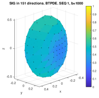
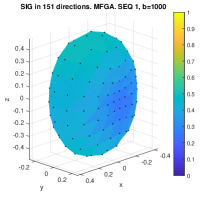
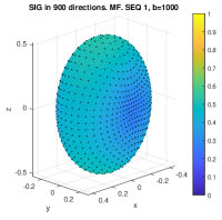
((a)) SEQ1, $b=1000\,\text{s/mm}^{2}$.

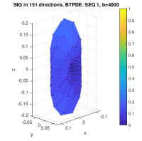
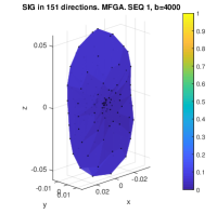
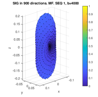
((b)) SEQ1, $b=4000\,\text{s/mm}^{2}$.

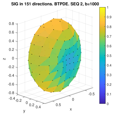
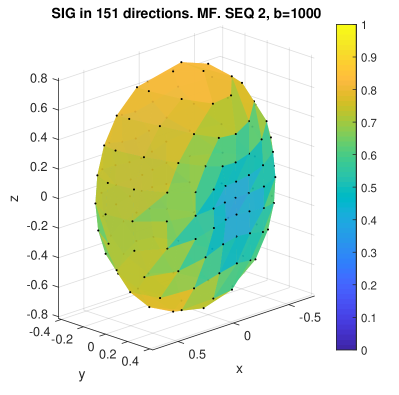
((c)) SEQ2, $b=1000\,\text{s/mm}^{2}$.

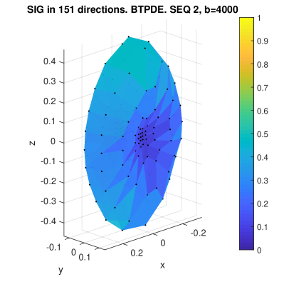
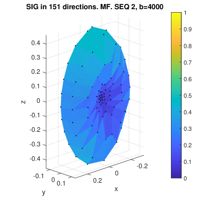
((d)) SEQ2, $b=4000\,\text{s/mm}^{2}$.

Figure 1: BTPDE signals, $S^{\text{BTPDE}}/S_{0}$, in 151 diffusion-encoding directions. MF signals, $S^{\text{MF}}/S_{0}$, in 151 diffusion-encoding directions. MFGA signals, $S^{\text{MFGA}}/S_{0}$, in 151 diffusion-encoding directions. MF signals, $S^{\text{MF}}/S_{0}$, in 900 diffusion-encoding directions. The black points indicate the diffusion-encoding direction, multiplied by the magnitude of the signal attenuation. The color indicates the value of the signal attenuation. SEQ1 is (PGSE, $\delta=10.6\text{ms},\Delta=13\text{ms}$), SEQ2 is (PGSE, $\delta=10.6\text{ms},\Delta=73\text{ms}$). The geometry is the pyramidal neuron 02b_pyramidal1aACC.

To verify numerically that the Matrix Formalism signal is close to the reference signal, we compute the signal differences between $S^{\text{MF}}$ and the reference $S^{\text{BTPDE}}$ over $30$ diffusion-encoding directions:

$$E(f,b)=\frac{\sum_{j=1}^{30}\left(S^{\text{MF}}(f,{\bm{g}}_{j})-S^{\text{BTPDE}}(f,{\bm{g}}_{j})\right)^{2}}{\sum_{j=1}^{30}\left(S^{\text{BTPDE}}(f,{\bm{g}}_{j})\right)^{2}}.$$ (23)

The directions are uniformly distributed on the unit sphere. The signal differences are {1.6%,2.2%,0.6%,1.9%} in order of {(SEQ1, $b=1000\,\text{s/mm}^{2}$), (SEQ1, $b=4000\,\text{s/mm}^{2}$), (SEQ2, $b=1000\,\text{s/mm}^{2}$), (SEQ2, $b=4000\,\text{s/mm}^{2}$)}. Thus, we consider the Matrix Formalism signal with the full set of 336 computed eigenvalues to be a good approximation of the reference signal.

3.2 The contribution of each eigenmode to the signal

Because $S^{\text{MF}}$ contains the contributions of all the computed eigenmodes in the requested interval, to get an idea of the importance of each eigenmode, we computed the signal difference that results when one eigenmode is removed, compared to using the full set of computed eigenmodes. This signal difference is computed for each sequence and each b-value, averaged over 30 gradient directions. The directions are uniformly distributed on the unit sphere. For the eigenfunction $i$, the signal difference is obtained as:

$$E^{\text{RM},i}(f,b)=\frac{\sum_{j=1}^{30}\left(S^{\text{MF}}(f,{\bm{g}}_{j})-S^{\text{MF},\text{RM},i}(f,{\bm{g}}_{j})\right)^{2}}{\sum_{j=1}^{30}\left(S^{\text{MF}}(f,{\bm{g}}_{j})\right)^{2}}.$$ (24)

The signal $S^{\text{MF}}$ uses the full set of computed eigenfunctions, the signal $S^{\text{MF},\text{RM},i}$ excludes the $i$th eigenfunction. In the following the signal differences will be given for two sequences at 2 b-values, in order of {(SEQ1, $b=1000\,\text{s/mm}^{2}$), (SEQ1, $b=4000\,\text{s/mm}^{2}$), (SEQ2, $b=1000\,\text{s/mm}^{2}$), (SEQ2, $b=4000\,\text{s/mm}^{2}$)}. We expect the second value to be the highest and the third value to be the lowest. We denote the $i$th eigenfunction as "significant" if $E^{\text{RM},i}(f,b)$ is more than a certain threshold.

In Figure 2, we show the significant eigenmodes. To visualize the "diffusion direction" of the eigenmodes, we use a RGB (red, green, blue) color scale based on the values of the RGB vector ${\bm{c}}_{n}$ with three non-negative valued components:

$${\bm{c}}_{n}=\frac{\begin{bmatrix}|a_{1n}^{x}|,|a_{1n}^{y}|,|a_{1n}^{z}|\end{bmatrix}}{\sqrt{(a_{1n}^{x})^{2}+(a_{1n}^{y})^{2}+(a_{1n}^{z})^{2}}}.$$ (25)

The color indicated by the RGB vector ${\bm{c}}_{n}$ can be used to gauge the relative contribution of the eigenmode to the 3 principle diffusion directions, $x$, $y$, $z$. For SEQ1, the significant eigenmodes between $25\mu\text{m}\leq l_{s}\leq 50\mu\text{m}$ are mostly green, meaning they contribute to diffusion in the $y$ direction. Between $0\leq l_{s}\leq 25\mu\text{m}$, there are many more significant eigenmodes that are red, meaning they contribute principally to diffusion in the $x$ direction. There is only one mode that is blue, meaning it contributes significantly to diffusion in the $z$ direction. This is expected since this neuron lies principally in the $x-y$ plane. We see also that at the higher b-value, there are more significant eigenmodes and the signal differences are also higher, compared with the lower b-value. The most significant eigenmode is the one with length scale $l_{s}(\lambda_{n})=33\mu\text{m}$, it is most aligned to the $y$-direction. Figure 3(a) shows this eigenfunction and we see the length scale corresponds to the "wavelength" of the significant oscillations of the eigenfunction in the geometry. Among eigenmodes with longer length scales, $l_{s}>50\mu\text{m}$, there are a lot fewer significant eigenmodes than between $0\leq l_{s}\leq 50\mu\text{m}$ and they are mostly in the $y$ direction (being mostly green). The eigenmode corresponding to $l_{s}(\lambda_{n})=343.6\mu\text{m}$ is shown in Figure 3(b). Its removal will result in signal differences of {19.1%, 83.8%, 8.8%, 40.8%}. The "wavelength" of this mode can be seen to be longer (slower oscillation) than the mode with $l_{s}(\lambda_{n})=33\mu\text{m}$. For SEQ2, at the lower length scales, around $l_{s}=15\mu\text{m}$, many of the significant eigenmodes for SEQ1 are no longer significant. In Figure 3(c), we show the eigenmode that is blue which is significant for both SEQ1 and SEQ2, corresponding to $l_{s}=15.6\mu\text{m}$. This eigenmode is predominately in the $z$-direction, and the rapid oscillations are found in the dendrite branches. The eigenfunction which has the longest spatial scale of $l_{s}=405\mu\text{m}$, shown in Figure 3(d), results in the following signal differences when it is removed: $E^{\text{RM},i}=\{1.06\%,6.58\%,0.57\%,1.22\%\}$.

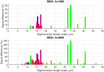
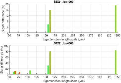
((a)) SEQ1 is (PGSE, $\delta=10.6\text{ms},\Delta=13\text{ms}$);

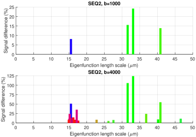
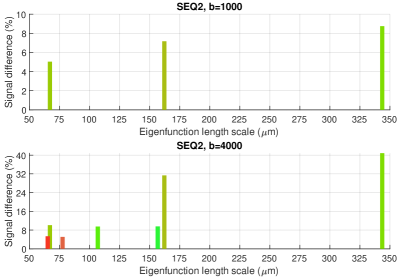
((b)) SEQ2 is (PGSE, $\delta=10.6\text{ms},\Delta=73\text{ms}$);

Figure 2: The signal differences due to the removal of each eigenmode, compared to using the full set of 336 eigenmodes. The eigenvalues have been converted to a length scale $l_{s}(\lambda_{n})$. The color indicates the "diffusion direction" of the eigenmodes, based on the values of the RGB vector ${\bm{c}}_{n}$ which is related to ${\bm{a}}_{1n}$. The geometry is the pyramidal neuron 02b_pyramidal1aACC.

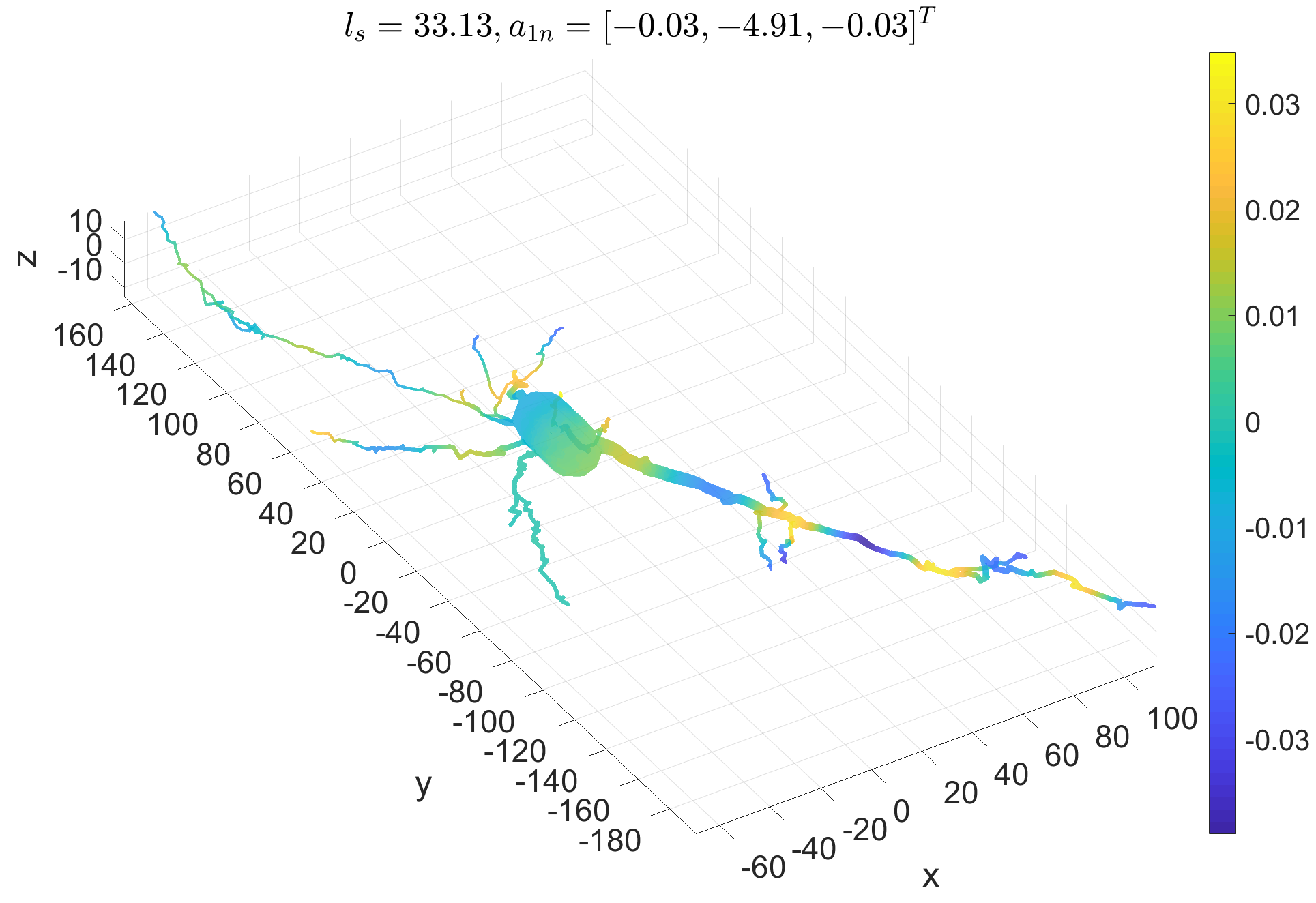
((a))

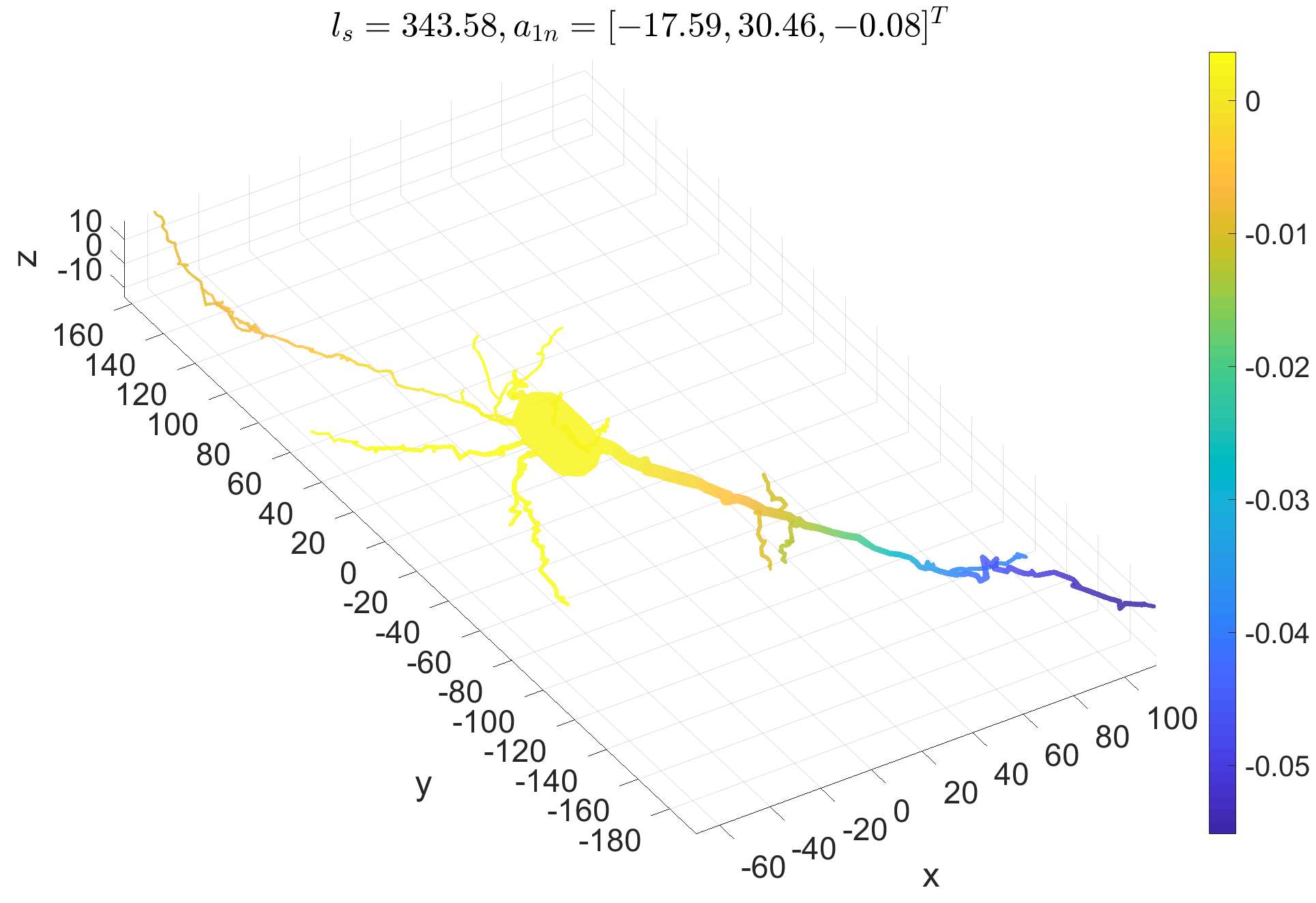
((b))

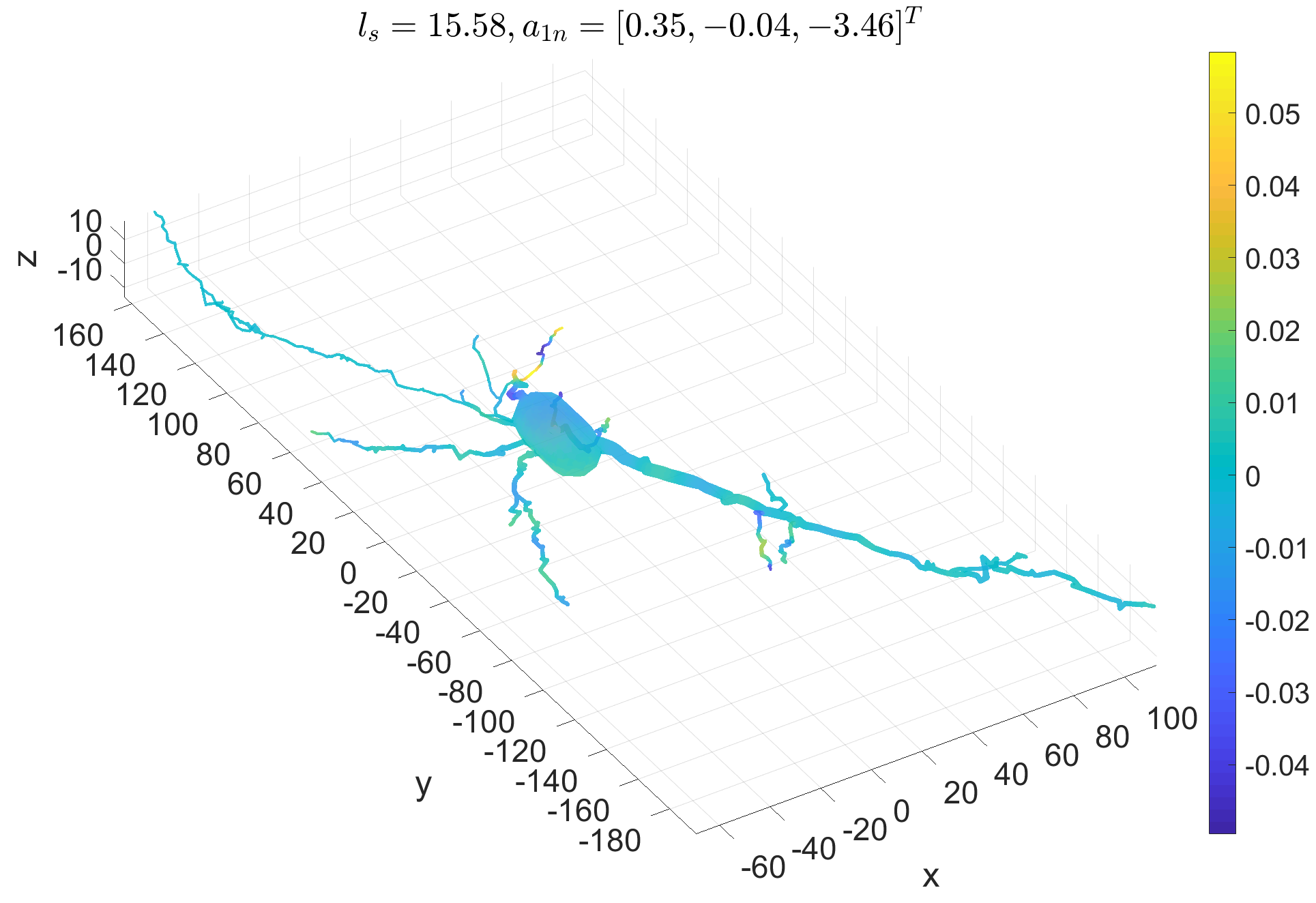
((c))

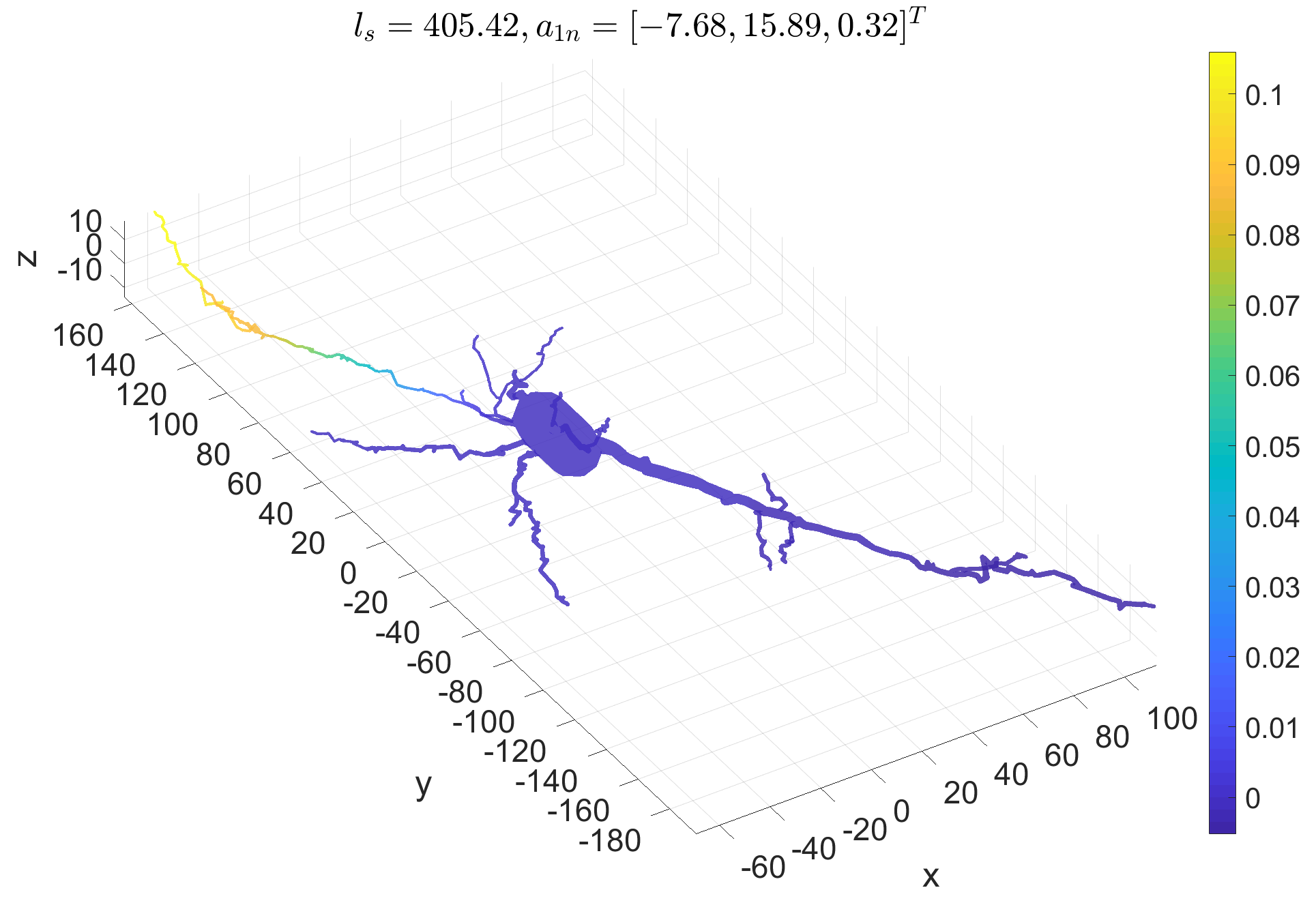
((d))

Figure 3: The eigenfunctions corresponding to the spatial scale of $l_{s}(\lambda_{n})=33\mu\text{m}$ (a), $343.6\mu\text{m}$ (b), $15.6\mu\text{m}$ (c) and $405\mu\text{m}$ (d). The geometry is the pyramidal neuron 02b_pyramidal1aACC.

In Table 1 we summarize the number of "significant" modes given the threshold of $E^{\text{RM},i}\geq 0.1\%$ and $E^{\text{RM},i}\geq 1\%$. Then we computed the Matrix Formalism signal using only the "significant" modes and compared it to the reference signal $S^{\text{BTPDE}}$ over 30 gradient directions. The number of significant modes range from 27 to 197, the signal errors compared to the reference signal range from less than 2% to 12%.

	Num of	Sig error	Num of	Sig error
	significant	from Ref	significant	from Ref
	modes (a)	(a)	modes (b)	(b)
SEQ1, $b=1000$	123	0.5%	53	12%
SEQ1, $b=4000$	197	1.0%	146	12%
SEQ2, $b=1000$	55	0.6%	27	9%
SEQ2, $b=4000$	107	2.1%	58	5%

Table 1: Significant modes are those whose removal leads to a signal difference of more than $0.1\%$ (a) or $1\%$ (b) compared to the signal from using the entire set of computed modes. In total, 336 eigenfunctions were computed. Signal error is the difference between the MF signal obtained using the indicated number of significant modes compared to the reference signal obtained from solving the Bloch-Torrey PDE. The signal difference is averaged over 30 diffusion-encoding directions, uniformly distributed on the sphere. The geometry is the pyramidal neuron 02b_pyramidal1aACC.

In Table 2 we give the computational times. All the simulations were performed on a server computer with 12 processors (Intel (R) Xeon (R) E5-2667 @2.90 GHz), 192 GB of RAM, running CentOS 7, using MATLAB R2019a. It is clear that once the eigendecomposition has been computed, the Matrix Formalism signal representation can be obtained rapidly for many sequences, b-values, and gradient directions. We note that given $n$ eigenfunctions, the number of associated model parameters of the Matrix Formalism representation is $n+3n(n-1)/2$, because the matrix $L$ is diagonal and the three matrices $A^{i}$, $i=x,y,z$, are symmetric. The number of parameters in each Matrix Formalism representation is also given in Table 2.

	MF	MF	BTPDE
Model size	336 modes	197 modes	44908 nodes
	61656 params	19503 params	171017 elem
Eigen solve	1095 sec	1095 sec
SEQ1, $b=1000$	0.09 sec	0.04 sec	26 sec
SEQ1, $b=4000$	0.09 sec	0.04 sec	39 sec
SEQ2, $b=1000$	0.12 sec	0.05 sec	22 sec
SEQ2, $b=4000$	0.13 sec	0.05 sec	30 sec

Table 2: The computational times to calculate the signals due to the indicated diffusion-encoding sequences at the indicated b-values, averaged over 30 diffusion-encoding directions. The geometry is the pyramidal neuron 02b_pyramidal1aACC.

3.3 Eigenvalues and eigenfunctions of the Bloch-Torrey operator

At high gradient amplitudes, it was demonstrated^{65, 66} in certain geometries (intervals, disks, spheres and the exterior of arrays of disks), the magnetization solution of the Bloch-Torrey equation exhibits localization near boundaries and interfaces. The analysis in those papers was based on the eigenfunctions of the complex-valued Bloch-Torrey operator,

$$-\left(\mathcal{D}_{0}\nabla^{2}-{\mathbb{i}}\gamma{\bm{g}}\cdot{\bm{x}}\right),$$

in contrast to the Laplace operator $-\mathcal{D}_{0}\nabla^{2}$. In the Appendix B, we show that the conversion between the eigenfunctions of the Bloch-Torrey operator $\{\psi_{j}\}$ and the eigenfunctions of the Laplace operator $\{\phi_{j}\}$ is given by

$$\begin{split}[\psi_{1}({\bm{x}}),\cdots\psi_{N_{eig}}({\bm{x}})]^{T}&=V^{-1}[\phi_{1}({\bm{x}}),\cdots\phi_{N_{eig}}({\bm{x}})]^{T}\\ V[\psi_{1}({\bm{x}}),\cdots\psi_{N_{eig}}({\bm{x}})]^{T}&=[\phi_{1}({\bm{x}}),\cdots\phi_{N_{eig}}({\bm{x}})]^{T}\end{split},$$ (26)

where the columns of $V$ contains the eigenvectors of the complex-valued matrix $K({\bm{g}})$. The eigenvalues of the Bloch-Torrey operator are exactly the eigenvalues of $K({\bm{g}})$. We remind the reader that the eigenvalues of $K({\bm{g}})$,

$$\mu_{1},\cdots,\mu_{N_{eig}},\quad 0<\Re{\mu_{1}}\leq\cdots\leq\Re{\mu_{N_{eig}}},$$

are found on the diagonal of the matrix $\Sigma$. We order the Bloch-Torrey (BT) eigenvalues and eigenfunctions by the magnitude of the real part of $\mu_{i}$, all of which are strictly greater than $0$.

In this section, we simulate the spindle neuron 03b_spindle4aACC. We compute $\psi_{1},\cdots,\psi_{N_{eig}}$ using the transformation above. To better visualize the "localized" nature of the BT eigenfunctions, in the Figures, we only indicate the support of $\psi_{i}({\bm{x}})$:

$$\text{supp}_{\psi,\epsilon}\equiv\{{\bm{x}}:|\psi({\bm{x}})|\geq 0.01\max_{{\bm{x}}}|\psi|\},$$

i.e., the region in space where it attains at least 1% of its maximum value. We do not indicate the actual values of $\psi$ inside its support.

In Figure 4(a), at the gradient amplitude $|{\bm{g}}|=0.0749$T/m, we show the supports of the BT eigenfunctions numbered 1, 2, 4, 5. We see the support of $\psi_{5}$ lies mostly in the soma. The supports of $\psi_{1}$, $\psi_{2}$, $\psi_{4}$ lie on the dendrite branches. The support of $\psi_{3}$ (lying on the dendrite branches) is not shown to avoid overlapping support regions in the plot. The non-zero values of the magnetization at $T_{E}$ show the locations of the supports of BT eigenfunctions 1, 2, 4, 5. In Figure 4(b), at the gradient amplitude $|{\bm{g}}|=0.3745$T/m, the supports of the BT eigenfunctions numbered 1, 2, 5, 6 all lie on the dendrites. The supports of $\psi_{3}$ and $\psi_{4}$ (lying on the dendrite branches) are not shown to avoid overlapping regions in the plot. The non-zero values of the magnetization show the locations of the supports of these eigenfunctions.

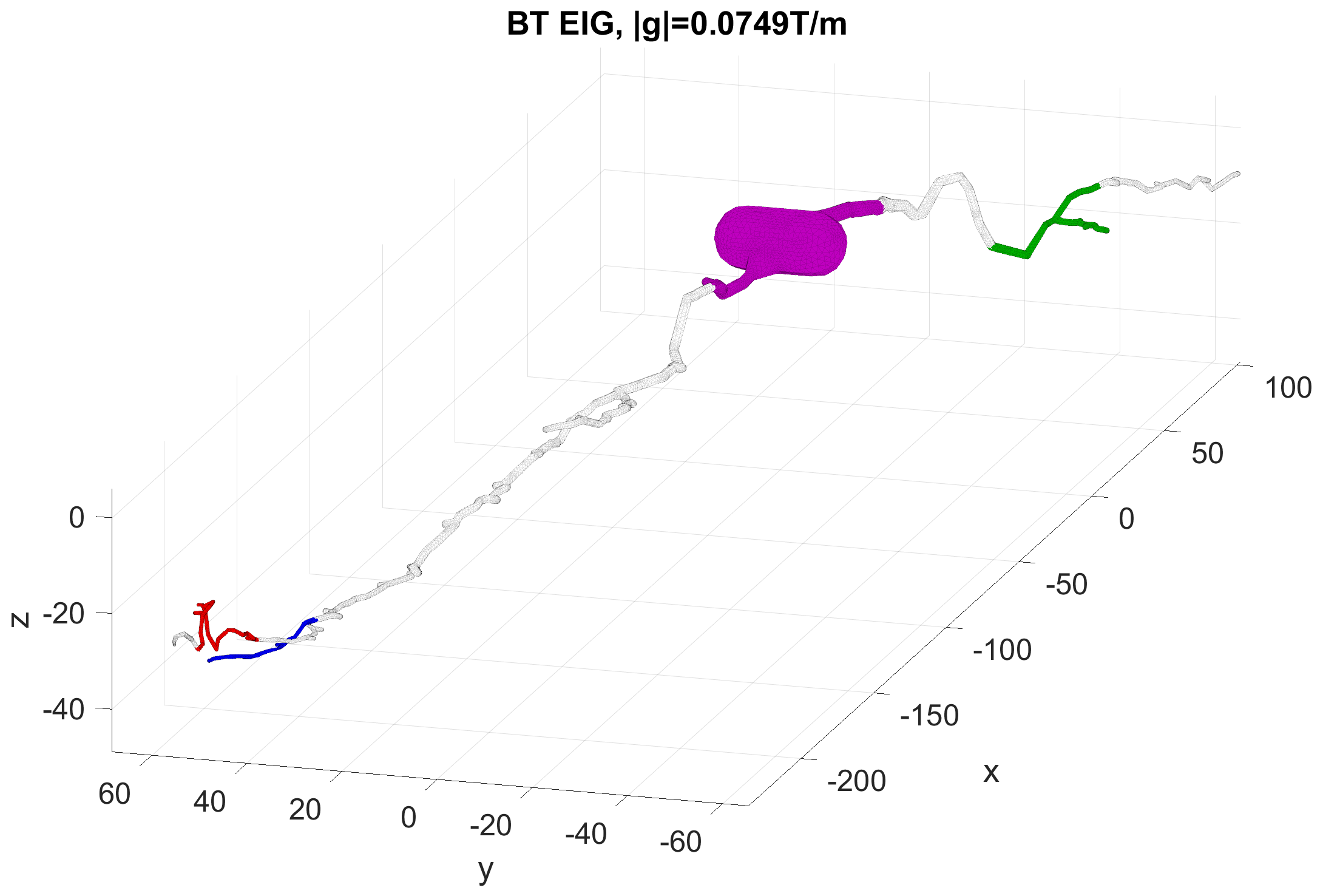
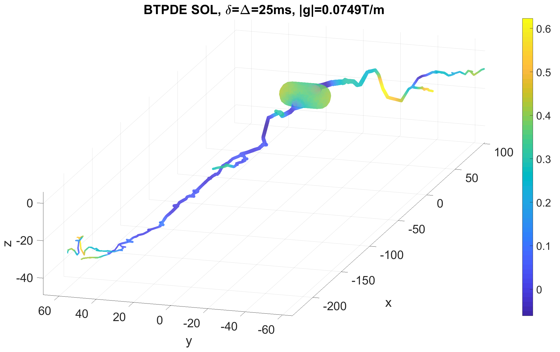
((a)) $|{\bm{g}}|=0.075\text{T/m}$

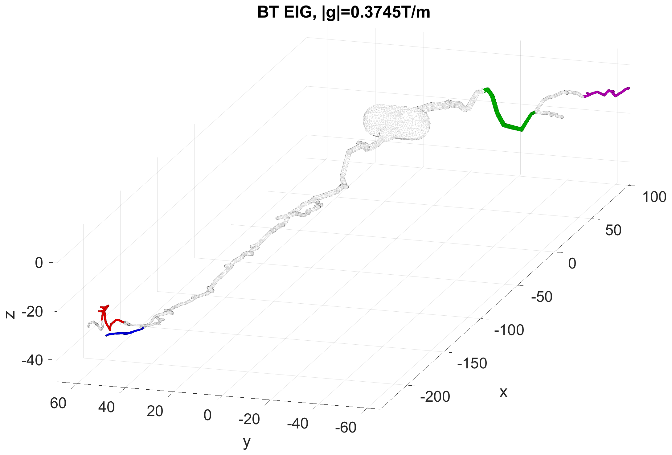
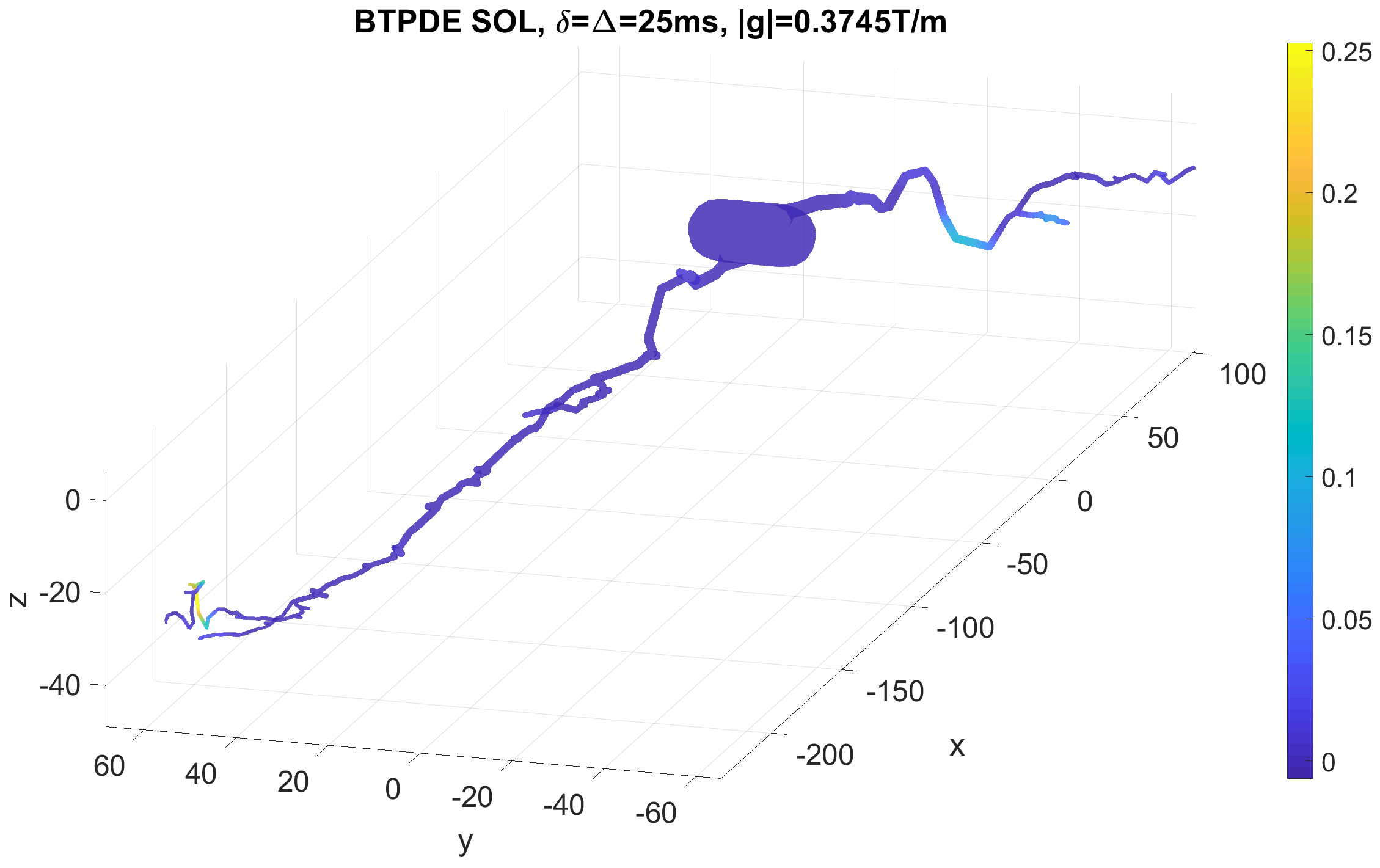
((b)) $|{\bm{g}}|=0.3745\text{T/m}$

Figure 4: (a) The gradient amplitude is $|{\bm{g}}|=0.075\text{T/m}$. Left: the supports of the first few BT eigenfunctions, ${\psi_{1}}$ (red), ${\psi_{2}}$ (green), ${\psi_{4}}$ (blue), ${\psi_{5}}$ (violet). Right: the magnetization at $T_{E}=\delta+\Delta$, where $\delta=\Delta=25\text{ms}$. (b) The gradient amplitude is $|{\bm{g}}|=0.3745\text{T/m}$. Left: the supports of the first few BT eigenfunctions, ${\psi_{1}}$ (red), ${\psi_{2}}$ (green), ${\psi_{5}}$ (blue), ${\psi_{6}}$ (violet). Right: the magnetization at $T_{E}=\delta+\Delta$, where $\delta=\Delta=25\text{ms}$. The BT eigenfunction index is in order of the magnitude of the real part. The gradient direction is ${\bm{u_{g}}}=[0.7071\ \ 0\ \ 0.7071]$. The geometry is the neuron 03b_spindle4aACC.

Next, we projected the initial spin density, $\rho$, which is the constant function, onto the BT eigenfunctions:

$$\rho\sqrt{|\Omega|}\left(V_{11}\psi_{1}+\cdots+V_{1N_{eig}}\psi_{N_{eig}}\right).$$

The projection coefficients are proportional to the first row of the matrix $V$. We normalized the BT eigenfunctions so that they have unit $L^{2}$ norm (integral of the square of the function over the geometry). We call a BT eigenfunction $\psi_{j}$ significant if

$$|V_{1j}|\geq 0.01.$$

In Figure 5 we show the complex eigenvalues of the significant BT eigenfunctions. We see that at the higher gradient amplitude, the significant BT eigenvalues have a wider range in both their real parts as well as their imaginary parts, than at the smaller gradient amplitude. In terms of the magnetization, a larger range of the real part indicates faster transient dynamics during the gradient pulses, and a larger range of the imaginary part indicates more time oscillations.

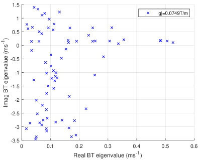
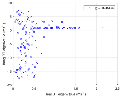
Figure 5: The significant BT eigenvalues after the projection of the initial spin density onto the space of BT eigenfunctions. The real part of the BT eigenvalues are plotted against the imaginary part. The gradient direction is ${\bm{u_{g}}}=[0.7071\ \ 0\ \ 0.7071]$. Left: $|{\bm{g}}|=0.075\text{T/m}$. Right: $|{\bm{g}}|=0.3745\text{T/m}$. The geometry is the neuron 03b_spindle4aACC.

3.4 Length scale range of Laplace eigenfunctions

To investigate the question of what range of Laplace eigenvalues is sufficient to accurately describe the diffusion MRI signal, we computed $S^{\text{BTPDE}}$ and $S^{\text{MF}}$ for the neuron 03b_spindle4aACC on two finite elements meshes, a fine mesh with 44201 nodes and 160205 elements, and a coarser mesh with 17370 nodes and 56163 elements. The $S^{\text{MF}}$ on these two FE meshes were computed with 4 choices of $l_{s}^{min}$: $4\mu\text{m}$, $2\mu\text{m}$, $1\mu\text{m}$ and $0.5\mu\text{m}$. The $S^{\text{BTPDE}}$ on the finer mesh is considered the reference solution and we show in Table 3 the mean relative signal error between the various simulations and the reference solution, averaged over the 6 gradient directions. Two gradient amplitudes and three PGSE sequences (with $\delta=\Delta$, $\delta=2.5\text{ms},10\text{ms},25\text{ms}$) were simulated, making a range of b-values from $4.2\,\text{s/mm}^{2}$ to $10416\,\text{s/mm}^{2}$. We see that on the coarser finite elements mesh, the mean relative error is less than $4.1\%$ for $S^{\text{MF}}$ with $l_{s}^{min}=4\mu\text{m}$ and it is less than $5.4\%$ for $S^{\text{MF}}$ with $l_{s}^{min}=0.5\mu\text{m}$ for the entire range of b-values. On the fine finite elements mesh, the mean relative errors are less than $2.6\%$, $1.3\%$, $1.6\%$, $1.6\%$ for $S^{\text{MF}}$ with $4\mu\text{m}$, $2\mu\text{m}$, $1\mu\text{m}$ and $0.5\mu\text{m}$, respectively. Some small increase in the mean relative errors are probably due to numerical errors of the eigenvalue computations.

Gradient	Pulse	b-value	BTPDE-h (REF)	Mean relative error with respect to BTPDE-h (REF) (%)
amplitude	duration	($\,\text{s/mm}^{2}$)	Mean signal/$S_{0}$	MF-H 4	MF-H 0.5	BTPDE-H	MF-h 4	MF-h 2	MF-h 1	MF-h 0.5
$0.075$ T/m	$2.5$ ms	4.2	0.995	0.0	0.0	0.0	0.0	0.0	0.0	0.0
	$10$ ms	267	0.829	0.4	0.5	0.0	0.1	0.1	0.1	0.1
	$25$ ms	4167	0.262	2.4	2.6	0.2	0.6	0.7	0.7	0.7
$0.3745$ T/m	$2.5$ ms	104	0.884	0.3	0.6	0.1	0.1	0.1	0.1	0.1
	$10$ ms	6667	0.073	4.1	5.4	0.3	0.9	1.3	1.6	1.6
	$25$ ms	104167	0.009	1.9	2.2	1.1	2.6	0.7	0.9	1.1

Table 3: Diffusion MRI signals were simulated in 6 gradient directions, uniformly distributed in the unit semi-sphere. The reference signal, denoted BTPDE-h, is the BTPDE signal on the finely discretized finite element mesh (44201 nodes, 160205 elements), with ODE solver tolerances $atol=10^{-6}$, $rtol=10^{-4}$. The mean signal is the averaged signal over the 6 gradient directions. The mean relative error is the relative difference between the various simulations and the reference signal BTPDE-h, averaged over the 6 gradient directions. The simulation denoted as BTPDE-H is the BTPDE solution on a coarser finite elements mesh (17370 nodes, 56163 elements) with the same ODE solver tolerances. Two Matrix Formalism simulations on the coarse FE mesh are denoted "MF-H 4" ($l_{s}^{min}=4\mu\text{m}$, 166 eigenfunctions) and "MF-H 0.5" ($l_{s}^{min}=0.5\mu\text{m}$, 5498 eigenfunctions). Four Matrix Formalism simulations on the fine FE mesh are denoted "MF-h 4" ($l_{s}^{min}=4\mu\text{m}$, 170 eigenfunctions), "MF-h 2" ($l_{s}^{min}=2\mu\text{m}$, 507 eigenfunctions), "MF-h 1" ($l_{s}^{min}=1\mu\text{m}$, 2082 eigenfunctions), and "MF-h 0.5" ($l_{s}^{min}=0.5\mu\text{m}$, 9093 eigenfunctions). The geometry is the neuron 03b_spindle4aACC.

To provide an at-a-glance summary of the significant BT and Laplace eigenfunctions at the end of the first gradient pulse $t=\delta$, we computed the matrix

$$A(\delta)=\begin{bmatrix}V_{11}e^{-\mu_{1}\delta}&&&&\\ &V_{12}e^{-\mu_{2}\delta}&&&\\ &&&\ddots&\\ &&&&V_{1N_{eig}}e^{-\mu_{N_{eig}}\delta}\end{bmatrix}V^{-1},\quad A(\delta)\in\mathbb{C}^{N_{eig}\times N_{eig}},$$

for the neuron 03b_spindle4aACC at two gradient amplitudes and two values of $\delta$. It is easy to see that the magnetization solution at $t=\delta$ is

$$M({\bm{x}},\delta)=\rho\sqrt{|\Omega|}\left(V_{11}e^{-\mu_{1}\delta}\psi_{1}({\bm{x}})+\cdots+V_{1N_{eig}}e^{-\mu_{N_{eig}}\delta}\psi_{N_{eig}}({\bm{x}})\right),$$

where we time evolved the BT eigenfunctions according to their eigenvalues. One can project $M({\bm{x}},\delta)$ onto the space of the Laplace eigenfunctions:

$$M({\bm{x}},\delta)=\rho\sqrt{|\Omega|}\left(c_{1}(\delta)\phi_{1}({\bm{x}})+\cdots+c_{N_{eig}}(\delta)\phi_{N_{eig}}({\bm{x}})\right).$$ (27)

The sum of $A(\delta)$ along the $k$th column is exactly $c_{k}(\delta)$. In Figure 6, we show the indices $j$ and $k$ such that $|A_{jk}(\delta)|\geq 0.001$ for three choices of gradient amplitudes and pulse durations. This threshold was made so that the resulting signal is within 1% of the signal where no entries of $A(\delta)$ were zeroed out. The row index of $A(\delta)$ is the index of the BT eigenfunction, the column index of $A(\delta)$ is the index of the Laplace eigenfunction. The value of the $j$th row and the $k$th column, $A_{jk}(\delta)$, is the projection onto the $k$th Laplace eigenfunction of the time evolved $j$th BT eigenfunction, $V_{1j}e^{-\mu_{j}\delta}\psi_{j}({\bm{x}})$. We see a clear reduction of the number of significant BT eigenfunctions as $\delta$ increases. At the higher gradient amplitude, there are a larger number of significant BT eigenfunctions as well as a larger number of Laplace eigenfunctions. At $\delta=2.5\text{ms}$, the minimum significant Laplace eigenfunction length scale went from $3.5\mu\text{m}$ to $2.4\mu\text{m}$ as $|{\bm{g}}|$ was increased from $0.075\text{T/m}$ to $0.3745\text{T/m}$. Finally, we caution that $|c_{k}(\delta)|=|\sum_{j}A_{jk}(\delta)|$ can be significantly smaller than $\sum_{j}|A_{jk}(\delta)|$ due to cancellations of numbers of opposite signs. This means non-zero columns in Figure 6 may have a coefficient $c_{k}(\delta)$ that is negligible.

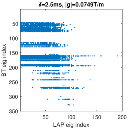
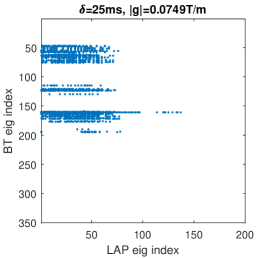
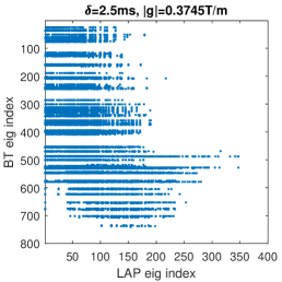
Figure 6: The magnetization at $t=\delta$ is projected onto the space of BT eigenfunctions, each of which is projected onto the Laplace eigenfunctions. The matrix that contains the projection coefficients of the time-evolved BT eigenfunctions onto the Laplace eigenfunctions is shown here. If the projection of the time-evolved $i$th BT eigenfunction onto the $j$th Laplace eigenfunction has a magnitude greater than 0.001, it is marked by a blue dot in the $i$th row and $j$ column. The BT and Laplace eigenfunction indices are ordered by the real part of their eigenvalues. Left: $|{\bm{g}}|=0.075\text{T/m}$, $\delta=\Delta=2.5\text{ms}$, $b=4.17\,\text{s/mm}^{2}$, the maximum BT index is 334, corresponding to the eigenvalue of $\mu=(3.3+0.1{\mathbb{i}})\text{ms}^{-1}$, the maximum LAP index is 199, corresponding to the length scale of $3.5\mu\text{m}$. Middle: $|{\bm{g}}|=0.075\text{T/m}$, $\delta=\Delta=25\text{ms}$, $b=4167\,\text{s/mm}^{2}$ the maximum BT index is 195, corresponding to the eigenvalue of $\mu=(1.6-3.0{\mathbb{i}})\text{ms}^{-1}$, the maximum LAP index is 137, corresponding to the length scale of $4.6\mu\text{m}$. Right: $|{\bm{g}}|=0.3745\text{T/m}$, $\delta=\Delta=25\text{ms}$, $b=104.2\,\text{s/mm}^{2}$, the maximum BT index is 752, corresponding to the eigenvalue of $\mu=(8.9+3.3{\mathbb{i}})\text{ms}^{-1}$, the maximum LAP index is 347, corresponding to the length scale of $2.4\mu\text{m}$. The geometry is the neuron 03b_spindle4aACC. The gradient direction is ${\bm{u_{g}}}=[0.7071\ \ 0\ \ 0.7071]$.

3.5 Simulation of the apparent diffusion coefficient

As an additional validation of our computations of the Matrix Formalism signal, we compare the ADC from the Matrix Formalism signal with several other computation methods. The first method is a linear fit of the BTPDE signal at two small $b$-values, which we chose to be $b=0\,\text{s/mm}^{2}$ and $b=1\,\text{s/mm}^{2}$. The second method uses the HADC model⁶² which is derived from the BTPDE using mathematical homogenization. The HADC model is a PDE model whose solution gives the time-dependent and gradient direction-dependent effective diffusion coefficient for arbitrary diffusion encoding sequences. The third method is an analytical short time approximation formula for the ADC. A well-known formula for the ADC in the short diffusion time regime is the following short time approximation (STA) ^{67, 68}:

$$STA=\mathcal{D}_{0}\left(1-\frac{4\sqrt{\mathcal{D}_{0}}}{3\;\sqrt{\pi}}\sqrt{\Delta}\frac{{A}}{dim\;V}\right),$$

where $\dfrac{A}{V}$ is the surface to volume ratio and $\mathcal{D}_{0}$ is the intrinsic diffusivity coefficient. In the above formula the pulse duration $\delta$ is assumed to be very small compared to $\Delta$. A recent correction to the above formula ⁶², taking into account the finite pulse duration $\delta$ and the gradient direction ${\bm{u_{g}}}$, is the following:

$$STA=\mathcal{D}_{0}\left[1-\frac{4\sqrt{\mathcal{D}_{0}}}{3\;\sqrt{\pi}}C_{\delta,\Delta}\frac{A_{\bm{u_{g}}}}{V}\right],$$ (28)

where

$$A_{\bm{u_{g}}}=\int_{\partial\Omega}\left({\bm{u_{g}}}\cdot{\bm{n}}\right)^{2}\,ds$$

is gradient direction dependent, and

$$C_{\delta,\Delta} =\dfrac{4}{35}\dfrac{\left(\Delta+\delta\right)^{7/2}+\left(\Delta-\delta\right)^{7/2}-2\left(\delta^{7/2}+\Delta^{7/2}\right)}{\delta^{2}\left(\Delta-\delta/3\right)}=\sqrt{\Delta}\left(1+\dfrac{1}{3}\dfrac{\delta}{\Delta}-\dfrac{8}{35}\left(\dfrac{\delta}{\Delta}\right)^{3/2}+\cdots\right).$$

When $\delta\ll\Delta$, the value $C_{\delta,\Delta}$ is approximately $\sqrt{\Delta}$.

We compute the Matrix Formalism ADC for the neuron 03b_spindle4aACC using $l_{s}^{min}=0.5\mu\text{m}$, on a finite element mesh with 44201 nodes and 160205 elements, this resulted in 9093 Laplace eigenfunctions. The BTPDE and the HADC simulations are also computed on this finite elements mesh, with ODE solver tolerances $atol=10^{-6}$, $rtol=10^{-4}$. Ten PGSE sequences were simulated with $\Delta=2\delta$, where $\delta$ = $0.04\text{ms}$, $0.08\text{ms}$, $0.16\text{ms}$, $0.32\text{ms}$, $0.64\text{ms}$, $1.28\text{ms}$, $2.56\text{ms}$, $5.12\text{ms}$, $10.24\text{ms}$, $20.48\text{ms}$. In Figure 7, we see that the ADC from BTPDE and HADC are identical for all the 10 PGSE sequences. We see the STA matches them at the three shortest diffusion times, and the MF does not match them at the shortest 4 diffusion times, but starts to match them from the 5th diffusion time onwards. These results are not surprising given that the required number of Laplace eigenfunctions to accurately represent the diffusion Green’s function goes to infinity as the diffusion time goes to 0.

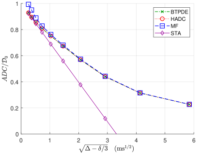
Figure 7: The computed apparent diffusion coefficient for PGSE sequences with $\Delta=2\delta$, where $\delta$ = $0.04\text{ms}$, $0.08\text{ms}$, $0.16\text{ms}$, $0.32\text{ms}$, $0.64\text{ms}$, $1.28\text{ms}$, $2.56\text{ms}$, $5.12\text{ms}$, $10.24\text{ms}$, $20.48\text{ms}$. The diffusion time is defined as $\Delta-\delta/3$. The BTPDE ADC is obtained uses a linear fit of the ADC from $b=0$ and $b=1\,\text{s/mm}^{2}$. The HADC model is a PDE model whose solution gives the time-dependent and gradient direction-dependent effective diffusion coefficient for arbitrary diffusion encoding sequences and it is derived from the BTPDE. The STA is an analytical formula for the time-dependent and gradient direction-dependent effective diffusion coefficient based on the surface area and the volume. The MF is the Matrix Formalism ADC using $l_{s}^{min}=0.5\mu\text{m}$. The BTPDE, the HADC, and the MF simulations are computed on a finite element mesh of (44201 nodes, 160205 elements), with ODE solver tolerances $atol=10^{-6}$, $rtol=10^{-4}$. For MF, this resulted in 9093 Laplace eigenfunctions. The gradient direction is ${\bm{u_{g}}}=[1\ \ 0\ \ 0]$. The geometry is the neuron 03b_spindle4aACC. The intrinsic diffusion coefficient is $\mathcal{D}_{0}=2\times 10^{-3}\,\text{mm}^{2}/\text{s}$.

4 Discussion

We have shown some of the functionalities of the Matrix Formalism Module within the diffusion MRI simulation toolbox SpinDoctor. We showed that the numerically computed $S^{\text{MF}}$ is very close to the reference signal from the Bloch-Torrey PDE for realistic neuron geometries at a wide range of b-values, and the agreement between the two are good at a wide range of diffusion times. We examined in detail the contributions of different eigenmodes at different diffusion times and different b-values. By choosing to represent the eigenvalues by a quantity of length $l_{s}(\lambda_{n})$, we highlighted the important spatial scales that contribute to the diffusion MRI signal. It can be seen that the longest length scales of the Laplace eigenfunctions roughly relate to the size of the geometry in the spatial directions. In addition, the length scale of a Laplace eigenfunction is related to the "wavelength" of the oscillations of the eigenfunction.

We have validated our Matrix Formalism computations by comparing it with the reference solution obtained from solving the BTPDE for a whole neuron. We showed that the $S^{\text{MF}}$ can be made more accurate by decreasing the requested minimum length scale $l_{s}^{min}$ and refining the finite elements mesh. We also showed through an ADC computation that, fixing the number of Laplace eigenfunctions a priori means that $S^{\text{MF}}$ cannot be made accurate at arbitrarily short diffusion times, since the number of required Laplace eigenfunctions, to describe the magnetization limit as the diffusion time goes to 0, goes to infinity.

We gave the transformation that link the Laplace eigenfunctions to the eigenfunctions of the Bloch-Torrey operator. We computed the BT eigenfunctions and eigenvalues for a whole neuron. We showed that at high enough gradient amplitude, the first few BT eigenfunctions (ordered by their real part) have support that are localized to a small region of the geometry. We showed the BT eigenvalues have a larger range in both their real part and imaginary part as the gradient amplitude increases. This explains the faster transient behavior and the oscillatory nature of the magnetization at high gradient amplitude. We showed that the higher indexed BT eigenfunctions have contributions from Laplace eigenfunctions that have shorter length scales.

There are two important advantages to the Matrix Formalism signal representation over the other representations. The first advantage is analytical, this representation makes explicit the link between the Laplace eigenvalues and eigenfunctions of the biological cell and its diffusion MRI signal. This clear link may help in the formulation of reduced models of the diffusion MRI signal that is closer to the physics of the problem. The second advantage is numerical, once the Laplace eigendecomposition has been computed and saved, the diffusion MRI signal can be calculated for arbitrary diffusion-encoding sequences and b-values at negligible additional cost. This will make it possible to use the Matrix Formalism as the inner loop of optimization procedures.

The need for a mathematically rigorous model of the diffusion MRI signal arising from realistic cellular structures was re-iterated in recent review papers ^{25, 26, 27}. Given that the Bloch-Torrey equation posed in realistic geometries is a gold-standard reference model of the diffusion MRI signal and the Matrix Formalism signal representation is equivalent to the reference model as long as enough eigenmodes are included, Matrix Formalism may be a possible bridge to formulating practical "inverse models" that can be used to robustly estimate biological relevant parameters from the acquired experimental data. In this paper, we moved Matrix Formalism a step closer to being a practically computable model and showed the number of significant eigenmodes is around a few hundred for realistic neurons. The next step may be searching for a unique set of "modes" onto which to project the eigenmodes of a population of many neurons in a voxel. Finding such a universal set of "modes" would require more advanced mathematical analysis on the diffusion operator in geometries with multiple length scales. A modified Fourier basis may be considered such as in ⁶⁹ as a possible future direction of research.

Currently, the Matrix Formalism Module allows the computation of the Matrix Formalism signal and the Matrix Formalism Gaussian Approximation signal for realistic neuron (impermeable membranes) with the PGSE sequence. Matrix Formalism for permeable membranes and for general diffusion-encoding sequences are under development and will be released in the future. The SpinDoctor toolbox and the Neuron Module have been developed in the MATLAB R2017b and require no additional MATLAB toolboxes. However, the current version of the Matrix Formalism Module requires the MATLAB PDE Toolbox (2017 or later) due to certain difficulties of implementing the matrix eigenvalue solution on a restricted eigenvalue interval. This technical issue will be addressed in a future release.

The Matrix Formalism Module follows the same workflow as SpinDoctor and the Neuron Module and builds upon the functionalities of SpinDoctor. To use the Matrix Formalism Module, it is necessary to read first the documentation of SpinDoctor. The source code, examples, documentation of SpinDoctor, the Neuron Module and the Matrix Formalism Module are available at https://github.com/jingrebeccali/SpinDoctor.

5 Conclusion

We presented a simulation module that we have implemented inside a MATLAB-based diffusion MRI simulator called SpinDoctor that efficiently computes the Matrix Formalism representation for realistic geometrical models of neurons. With this new simulation tool, we seek to bridge the gap between physical quantities closely related to the cellular geometrical structure, namely, its Laplace eigenfunctions, eigenvalues and their length scales, with the measured diffusion MRI signal. We hope this Matrix Formalism Module makes the mathematically rigorous signal representation into a practical model for the research community.

Appendix A Derivation of the Matrix Formalism signal representation

Let $\phi_{n}({\bm{x}})$ and $\lambda_{n}$, $n=1,\cdots$, be the $L^{2}$-normalized eigenfunctions and eigenvalues associated to the Laplace operator with homogeneous Neumann boundary conditions (the surface of the neurons are supposed impermeable):

$$-\nabla\mathcal{D}_{0}\left(\nabla\phi_{n}({\bm{x}})\right) =\lambda_{n}\phi_{n}({\bm{x}}), \quad{\bm{x}}\in\Omega,$$

$$\mathcal{D}_{0}\nabla\phi_{n}({\bm{x}})\cdot{\bm{\nu}}({\bm{x}}) =0, \quad{\bm{x}}\in\Gamma.$$

We assume the non-negative real-valued eigenvalues are ordered in non-decreasing order:

$$0=\lambda_{1}<\lambda_{2}\leq\lambda_{3}\leq\cdots$$

so that $\lambda_{1}=0$ (this means the first Laplace eigenfunction is the constant function). There is only one constant eigenfunction because we assume the neuron is a connected domain. Let $L$ be the diagonal matrix containing the first $N_{eig}$ Laplace eigenvalues:

$$L=\text{diag}[\lambda_{1},\lambda_{2},\cdots,\lambda_{N_{eig}}]\in\mathbb{R}^{N_{eig}\times N_{eig}}.$$ (29)

For the PGSE sequence, the time interval $[0,T_{E}],T_{E}=\delta+\Delta$ is separated into three subintervals:

$$f(t)=\begin{cases}1,\quad&t\in[0,\delta],\\ 0,\quad&t\in[\delta,\Delta],\\ -1,\quad&t\in[\Delta,T_{E}].\end{cases}$$ (30)

If $t\in[0,\delta]$, decompose the solution $M({\bm{x}},t)$ in the basis of $\{\phi_{n}({\bm{x}})\}$ as

$$M({\bm{x}},t)=\sum_{n=1}^{N_{eig}}T_{n}(t)\phi_{n}({\bm{x}})=[\phi({\bm{x}})]^{T}T(t),$$ (31)

where we define the space and time dependent column vectors

$$\phi({\bm{x}})=\begin{bmatrix}\phi_{1}({\bm{x}})\\ \vdots\\ \phi_{N_{eig}}({\bm{x}})\end{bmatrix},\ T(t)=\begin{bmatrix}T_{1}(t)\\ \vdots\\ T_{N_{eig}}(t)\end{bmatrix}.$$

Substituting into the original Bloch-Torrey equation, multiplying both sides with $\{\phi_{k}({\bm{x}})\}$ and integrating over $\Omega$ give

$$\frac{\partial}{\partial t}{T_{k}(t)}=-\lambda_{k}T_{k}(t)-{\mathbb{i}}\gamma\sum_{n=1}^{N_{eig}}T_{n}(t)\int_{\Omega}{\bm{g}}\cdot{\bm{x}}\phi_{n}({\bm{x}})\phi_{k}({\bm{x}})d{\bm{x}},\quad k=1,...,N_{eig}.$$ (32)

Let $W({\bm{g}})$ be the ${N_{eig}\times N_{eig}}$ matrix whose entries are:

$$W({\bm{g}})=\left[\int_{\Omega}{\bm{g}}\cdot{\bm{x}}\phi_{m}({\bm{x}})\phi_{n}({\bm{x}})d{\bm{x}}\right]=g_{x}A^{x}+g_{y}A^{y}+g_{z}A^{z}$$ (33)

where ${\bm{g}}=(g_{x},g_{y},g_{z}),$ and

$$A^{i}=\begin{bmatrix}a_{mn}^{i}\end{bmatrix},\quad i=\{x,y,z\},\quad 1\leq m,n\leq N_{eig},$$ (34)

are three symmetric ${N_{eig}\times N_{eig}}$ matrices whose entries are the first order moments in the coordinate directions of the product of pairs of eigenfunctions:

$$\begin{split}a_{mn}^{x}&=\int_{\Omega}x\phi_{m}({\bm{x}})\phi_{n}({\bm{x}})d{\bm{x}},\;\\ a_{mn}^{y}&=\int_{\Omega}y\phi_{m}({\bm{x}})\phi_{n}({\bm{x}})d{\bm{x}},\\ a_{mn}^{z}&=\int_{\Omega}z\phi_{m}({\bm{x}})\phi_{n}({\bm{x}})d{\bm{x}}.\end{split}$$

We define the complex-valued matrix $K({\bm{g}})$

$$K({\bm{g}})\equiv L+{\mathbb{i}}\gamma W({\bm{g}}).$$ (35)

Then the system of equations 32 can be written as

$$\frac{\partial}{\partial t}{T(t)}=-KT(t).$$ (36)

The solution to this system of linear differential equations is

$$T(t)=e^{-Kt}T(0),\ t\in[0,\delta].$$ (37)

The initial condition

$$M({\bm{x}},0)=\sum_{n=1}^{N_{eig}}T_{n}(0)\phi_{n}({\bm{x}})=[\phi({\bm{x}})]^{T}T(0),$$

gives us the initial coefficients

$$\ T_{n}(0)=\int_{\Omega}M({\bm{x}},0)\phi_{n}({\bm{x}})d{\bm{x}}.$$ (38)

We get

$$M({\bm{x}},t)=[\phi({\bm{x}})]^{T}e^{-Kt}T(0),\ t\in[0,\delta].$$ (39)

Similar analysis can be applied to the interval $[\delta,\Delta]$ with $f(t)=0$ and $M({\bm{x}},\delta)$ acting as the initial condition for the system of differential equations. At the end of this interval, the magnetization is represented as

$$M({\bm{x}},\Delta)=[\phi({\bm{x}})]^{T}e^{-L(\Delta-\delta)}e^{-K\delta}T(0).$$ (40)

The magnetization measured at the end of the second pulse is

$$M({\bm{x}},T_{E})=[\phi({\bm{x}})]^{T}e^{-K^{*}\delta}e^{-L(\Delta-\delta)}e^{-K\delta}T(0).$$ (41)

Denote $H({\bm{g}},f)=e^{-K^{*}\delta}e^{-L(\Delta-\delta)}e^{-K\delta}$ and $\Phi=\begin{bmatrix}\int_{\Omega}\phi_{1}({\bm{x}})d{\bm{x}}\\ \vdots\\ \int_{\Omega}\phi_{N_{eig}}({\bm{x}})d{\bm{x}}\end{bmatrix}$. Then the echo signal is computed by integrating $M({\bm{x}},T_{E})$ over $\Omega$:

$$S=\int_{\Omega}M({\bm{x}},T_{E})d{\bm{x}}=\Phi^{T}H({\bm{g}},f)T(0).$$ (42)

If $M({\bm{x}},0)=\rho$, where $\rho$ is the initial spin density, then $T(0)=\rho\Phi$. With homogeneous Neumann boundary conditions, the $L^{2}$-normalized eigenfunctions $\phi_{n}({\bm{x}})$ have the following property

$$\Phi_{n}=\int_{\Omega}\phi_{n}({\bm{x}})d{\bm{x}}=\begin{cases}\sqrt{|\Omega|},\quad&n=1,\\ 0,\quad&n\geq 2,\end{cases}$$ (43)

with, in particular, $\phi_{1}({\bm{x}})\equiv\sqrt{\frac{1}{|\Omega|}}$. The vector $\Phi$ has only one non-zero value in the first position. Eq. 42 is then reduced to

$$S=\rho|\Omega|H_{11}({\bm{g}},f)=S_{0}H_{11}({\bm{g}},f).$$ (44)

Note that since $K$ and $K^{*}$ are symmetric matrices, $e^{-K^{*}\delta}$ and $e^{-K\delta}$ are also symmetric; thus, we have:

$$H^{T}({\bm{g}},f)=\left[e^{-K\delta}\right]^{T}e^{-L(\Delta-\delta)}\left[e^{-K^{*}\delta}\right]^{T}=e^{-K\delta}e^{-L(\Delta-\delta)}e^{-K^{*}\delta}$$ (45)

Eq. 41 can be written as

$$M({\bm{x}},T_{E})=[T(0)]^{T}H^{T}({\bm{g}},f)\phi({\bm{x}})=[T(0)]^{T}e^{-K\delta}e^{-L(\Delta-\delta)}e^{-K^{*}\delta}\phi({\bm{x}}).$$ (46)

In Eq. 44 we can reverse the order of the matrix exponentials in $H({\bm{g}},f)$ and achieve the same echo signal:

$$S=S_{0}\left[e^{-K\delta}e^{-L(\Delta-\delta)}e^{-K^{*}\delta}\right]_{11}.$$ (47)

Appendix B Eigenvalues and eigenfunctions of the Bloch-Torrey operator

To relate the eigen-decomposition of the Laplace operator $-\mathcal{D}_{0}\nabla^{2}$ to the eigen-decomposition of the complex-valued Bloch-Torrey operator $-\left(\mathcal{D}_{0}\nabla^{2}-{\mathbb{i}}\gamma{\bm{g}}\cdot{\bm{x}}\right)$, we first define $\psi_{m}({\bm{x}})$ and $\mu_{m}$, $m=1,\cdots,N_{eig}$, to be the eigenfunctions and eigenvalues associated to the Bloch-Torrey operator subject to homogeneous Neumann boundary conditions:

$$-(\mathcal{D}_{0}\nabla^{2}-{\mathbb{i}}\gamma{\bm{g}}\cdot{\bm{x}})\psi_{m}({\bm{x}}) =\mu_{m}\psi_{m}({\bm{x}}), \quad{\bm{x}}\in\Omega,$$ (48)

$$\mathcal{D}_{0}\nabla\psi_{m}({\bm{x}})\cdot{\bm{\nu}}({\bm{x}}) =0, \quad{\bm{x}}\in\Gamma.$$ (49)

Representing $\psi_{m}({\bm{x}}),m=1,\cdots,N_{eig}$, in the basis of the Laplace eigenfunctions $\phi_{n}({\bm{x}}),n=1,\cdots,N_{eig}$:

$$\psi_{m}({\bm{x}})=\sum_{n=1}^{N_{eig}}c_{mn}\phi_{n}({\bm{x}}),\ m=1,...,N_{eig},$$ (50)

and putting it into Eq. 48,

$$-\sum_{n=1}^{N_{eig}}c_{mn}\mathcal{D}_{0}\nabla^{2}\phi_{n}({\bm{x}})+{\mathbb{i}}\gamma{\bm{g}}\cdot{\bm{x}}\sum_{n=1}^{N_{eig}}c_{mn}\phi_{n}({\bm{x}})=\mu_{m}\sum_{n=1}^{N_{eig}}c_{mn}\phi_{n}({\bm{x}}),$$ (51)

we get

$$\sum_{n=1}^{N_{eig}}c_{mn}\lambda_{n}\phi_{n}({\bm{x}})+{\mathbb{i}}\gamma{\bm{g}}\cdot{\bm{x}}\sum_{n=1}^{N_{eig}}c_{mn}\phi_{n}({\bm{x}})=\mu_{m}\sum_{n=1}^{N_{eig}}c_{mn}\phi_{n}({\bm{x}}).$$ (52)

Multiply both sides with $\phi_{k}({\bm{x}})$ and integrate over $\Omega$:

$$\lambda_{k}c_{mk}+{\mathbb{i}}\gamma\sum_{n=1}^{N_{eig}}c_{mn}\int_{\Omega}{\bm{g}}\cdot{\bm{x}}\phi_{n}({\bm{x}})\phi_{k}({\bm{x}})d{\bm{x}}=\mu_{m}c_{mk},\quad m,k=1,...,N_{eig}.$$ (53)

Then writing Eq. 53 as a matrix equation for $C=[c_{mk}]\in\mathbb{C}^{N_{eig}\times N_{eig}}$, where $m$ is the row index and $k$ is the column index:

$$C\left(L+{\mathbb{i}}\gamma W({\bm{g}})\right)=CK({\bm{g}})=\Sigma C.$$

We see that we can obtain $C$ and $\Sigma$ by diagonalizing the complex-valued matrix $K({\bm{g}})$:

$$K({\bm{g}})=V\Sigma V^{-1},$$ (54)

where the matrix $V$ has the eigenvectors in the columns and $\Sigma$ has the eigenvalues on the diagonal. We can obtain $C$ by setting it to

$$C\equiv V^{-1}.$$ (55)

The diagonalization of the complex conjugate of $K({\bm{g}})$ is

$$\left(K({\bm{g}})\right)^{*}=L-{\mathbb{i}}\gamma W({\bm{g}})=(V^{-1})^{*}\Sigma^{*}(V)^{*}.$$ (56)

At the end of the first gradient pulse, the magnetization is

$$M({\bm{x}},\delta)=\mathcal{M}_{0}^{\psi}e^{-\Sigma\delta}[\psi_{1}({\bm{x}}),\cdots\psi_{N_{eig}}({\bm{x}})]^{T},$$ (57)

where $\mathcal{M}_{0}^{\psi}\in\mathbb{C}^{1\times N_{eig}}$ is the vector of coefficients of the initial magnetization projected onto the eigenfunctions of $K({\bm{g}})$. Similarly, at the beginning of the second time interval, the magnetization is

$$M({\bm{x}},\Delta)=\mathcal{M}_{\delta}^{\phi}e^{-L(\Delta-\delta)}[\phi_{1}({\bm{x}}),\cdots\phi_{N_{eig}}({\bm{x}})]^{T},$$ (58)

where $\mathcal{M}_{\delta}^{\phi}\in\mathbb{C}^{1\times N_{eig}}$ is the vector of coefficients of the magnetization at $t=\delta$ projected onto the eigenfunctions of $L$. Finally, at the end of the second interval, the magnetization is

$$M({\bm{x}},\delta+\Delta)=\mathcal{M}_{\Delta}^{\tilde{\psi}}e^{-\Sigma^{*}\delta}[\tilde{\psi}_{1}({\bm{x}}),\cdots\tilde{\psi}_{N_{eig}}({\bm{x}})]^{T},$$ (59)

where $\mathcal{M}_{\Delta}^{{\tilde{\psi}}}\in\mathbb{C}^{1\times N_{eig}}$ is the vector of coefficients of the magnetization at $t=\Delta$ projected onto the eigenfunctions of $K({\bm{g}})^{*}$ (we denoted this $\tilde{\psi}$). The conversion between $\psi$ and $\phi$ is

$$\begin{split}[\psi_{1}({\bm{x}}),\cdots\psi_{N_{eig}}({\bm{x}})]^{T}&=V^{-1}[\phi_{1}({\bm{x}}),\cdots\phi_{N_{eig}}({\bm{x}})]^{T}\\ V[\psi_{1}({\bm{x}}),\cdots\psi_{N_{eig}}({\bm{x}})]^{T}&=[\phi_{1}({\bm{x}}),\cdots\phi_{N_{eig}}({\bm{x}})]^{T}\end{split}.$$ (60)

So

$$\mathcal{M}_{0}^{\psi}=\rho\sqrt{|\Omega|}[V_{11},\cdots,V_{1n}],$$ (61)

is the first row of $V$, and

$$\mathcal{M}_{\delta}^{\phi}=\mathcal{M}_{0}^{\psi}e^{-\Sigma\delta}V^{-1}.$$ (62)

The conversion between $\tilde{\psi}$ and $\phi$ is

$$\begin{split}[\tilde{\psi}_{1}({\bm{x}}),\cdots\tilde{\psi}_{N_{eig}}({\bm{x}})]^{T}&=V^{*}[\phi_{1}({\bm{x}}),\cdots\phi_{N_{eig}}({\bm{x}})]^{T}\\ (V^{-1})^{*}[\tilde{\psi}_{1}({\bm{x}}),\cdots\tilde{\psi}_{N_{eig}}({\bm{x}})]^{T}&=[\phi_{1}({\bm{x}}),\cdots\phi_{N_{eig}}({\bm{x}})]^{T}\end{split}$$ (63)

Thus,

$$\mathcal{M}_{\Delta}^{{\tilde{\psi}}}=\mathcal{M}_{\delta}^{\phi}e^{-L(\Delta-\delta)}(V^{-1})^{*}.$$ (64)

The final magnetization is therefore

$$M({\bm{x}},\delta+\Delta)=\rho\sqrt{|\Omega|}[V_{11},\cdots,V_{1n}]e^{-\Sigma\delta}V^{-1}e^{-L(\Delta-\delta)}(V^{-1})^{*}e^{-(\Sigma)^{*}\delta}V^{*}[\phi_{1}({\bm{x}}),\cdots\phi_{N_{eig}}({\bm{x}})]^{T}.$$ (65)

Since the first Laplacian eigenfunction is the constant function and it is orthogonal to all the other Laplacian eigenfunctions, the signal is

$$S=\int_{{\bm{x}}\in\Omega}M({\bm{x}},\delta+\Delta)d{\bm{x}}=\rho{|\Omega|}[V_{11},\cdots,V_{1n}]e^{-\Sigma\delta}V^{-1}e^{-L(\Delta-\delta)}(V^{-1})^{*}e^{-(\Sigma)^{*}\delta}[V_{11},\cdots,V_{1n}]^{*},$$ (66)

where we only kept the first column of $V^{*}$.

References

- 1 Hahn EL. Spin Echoes. Phys. Rev. 1950; 80: 580–594.
- 2 Stejskal EO, Tanner JE. Spin Diffusion Measurements: Spin Echoes in the Presence of a Time-Dependent Field Gradient. The Journal of Chemical Physics 1965; 42(1): 288–292. doi: 10.1063/1.1695690
- 3 Bihan DL, Breton E, Lallemand D, Grenier P, Cabanis E, Laval-Jeantet M. MR imaging of intravoxel incoherent motions: application to diffusion and perfusion in neurologic disorders.. Radiology 1986; 161(2): 401-407. PMID: 3763909.
- 4 Palombo M, Ligneul C, Najac C, et al. New paradigm to assess brain cell morphology by diffusion-weighted MR spectroscopy in vivo. Proceedings of the National Academy of Sciences 2016; 113(24): 6671–6676. doi: 10.1073/pnas.1504327113
- 5 Abe M, Fukuyama H, Mima T. Water diffusion reveals networks that modulate multiregional morphological plasticity after repetitive brain stimulation. Proceedings of the National Academy of Sciences 2014; 111(12): 4608–4613. doi: 10.1073/pnas.1320223111
- 6 Reveley C, Seth AK, Pierpaoli C, et al. Superficial white matter fiber systems impede detection of long-range cortical connections in diffusion MR tractography. Proceedings of the National Academy of Sciences 2015; 112(21): E2820–E2828. doi: 10.1073/pnas.1418198112
- 7 Novikov DS, Jensen JH, Helpern JA, Fieremans E. Revealing mesoscopic structural universality with diffusion. Proceedings of the National Academy of Sciences 2014; 111(14): 5088–5093. doi: 10.1073/pnas.1316944111
- 8 Metcalfe-Smith E, Meeus E, Novak J, Dehghani H, Peet A, Zarinabad N. Auto-regressive Discrete Acquisition Points Transformation for Diffusion Weighted MRI Data. IEEE Transactions on Biomedical Engineering 2019: 1-1. doi: 10.1109/TBME.2019.2893523
- 9 Dang S, Chaudhury S, Lall B, Roy PK. Tractography-Based Score for Learning Effective Connectivity From Multimodal Imaging Data Using Dynamic Bayesian Networks. IEEE Transactions on Biomedical Engineering 2018; 65(5): 1057-1068. doi: 10.1109/TBME.2017.2738035
- 10 Moutal N, Maximov II, Grebenkov DS. Probing surface-to-volume ratio of an anisotropic medium by diffusion NMR with general gradient encoding. IEEE Transactions on Medical Imaging 2019: 1-1. doi: 10.1109/TMI.2019.2902957
- 11 Christiaens D, Cordero-Grande L, Hutter J, et al. Learning Compact -Space Representations for Multi-Shell Diffusion-Weighted MRI. IEEE Transactions on Medical Imaging 2019; 38(3): 834-843. doi: 10.1109/TMI.2018.2873736
- 12 Assaf Y, Blumenfeld-Katzir T, Yovel Y, Basser PJ. Axcaliber: A method for measuring axon diameter distribution from diffusion MRI. Magn. Reson. Med. 2008; 59(6): 1347–1354.
- 13 Alexander DC, Hubbard PL, Hall MG, et al. Orientationally invariant indices of axon diameter and density from diffusion MRI. NeuroImage 2010; 52(4): 1374–1389.
- 14 Zhang H, Hubbard PL, Parker GJ, Alexander DC. Axon diameter mapping in the presence of orientation dispersion with diffusion MRI. NeuroImage 2011; 56(3): 1301–1315.
- 15 Zhang H, Schneider T, Wheeler-Kingshott CA, Alexander DC. NODDI: Practical in vivo neurite orientation dispersion and density imaging of the human brain. NeuroImage 2012; 61(4): 1000–1016.
- 16 Burcaw LM, Fieremans E, Novikov DS. Mesoscopic structure of neuronal tracts from time-dependent diffusion. NeuroImage 2015; 114: 18 - 37. doi: 10.1016/j.neuroimage.2015.03.061
- 17 Palombo M, Ligneul C, Valette J. Modeling diffusion of intracellular metabolites in the mouse brain up to very high diffusion-weighting: Diffusion in long fibers (almost) accounts for non-monoexponential attenuation. Magnetic Resonance in Medicine 2017; 77(1): 343–350. doi: 10.1002/mrm.26548
- 18 Palombo M, Ligneul C, Najac C, et al. New paradigm to assess brain cell morphology by diffusion-weighted MR spectroscopy in vivo. Proceedings of the National Academy of Sciences 2016; 113(24): 6671–6676. doi: 10.1073/pnas.1504327113
- 19 Ning L, Özarslan E, Westin CF, Rathi Y. Precise Inference and Characterization of Structural Organization (PICASO) of tissue from molecular diffusion. NeuroImage 2017; 146: 452 - 473. doi: 10.1016/j.neuroimage.2016.09.057
- 20 Fieremans E, Jensen JH, Helpern JA. White matter characterization with diffusional kurtosis imaging. NeuroImage 2011; 58(1): 177 - 188.
- 21 Panagiotaki E, Schneider T, Siow B, Hall MG, Lythgoe MF, Alexander DC. Compartment models of the diffusion MR signal in brain white matter: A taxonomy and comparison. NeuroImage 2012; 59(3): 2241–2254.
- 22 Jespersen SN, Kroenke CD, Astergaard L, Ackerman JJ, Yablonskiy DA. Modeling dendrite density from magnetic resonance diffusion measurements. NeuroImage 2007; 34(4): 1473–1486.
- 23 Santis] SD, Jones DK, Roebroeck A. Including diffusion time dependence in the extra-axonal space improves in vivo estimates of axonal diameter and density in human white matter. NeuroImage 2016; 130: 91 - 103. doi: https://doi.org/10.1016/j.neuroimage.2016.01.047
- 24 Lee HH, Fieremans E, Novikov DS. What dominates the time dependence of diffusion transverse to axons: Intra- or extra-axonal water?. NeuroImage 2018; 182: 500 - 510. doi: https://doi.org/10.1016/j.neuroimage.2017.12.038
- 25 Novikov DS, Fieremans E, Jespersen SN, Kiselev VG. Quantifying brain microstructure with diffusion MRI: Theory and parameter estimation. NMR in Biomedicine 2019; 32(4): e3998. doi: 10.1002/nbm.3998
- 26 Novikov DS, Kiselev VG, Jespersen SN. On modeling. Magnetic Resonance in Medicine 2018; 79(6): 3172–3193. doi: 10.1002/mrm.27101
- 27 Fieremans E, Lee HH. Physical and numerical phantoms for the validation of brain microstructural MRI: A cookbook. NeuroImage 2018; 182: 39 - 61. doi: https://doi.org/10.1016/j.neuroimage.2018.06.046
- 28 Rensonnet G, Scherrer B, Girard G, et al. Towards microstructure fingerprinting: Estimation of tissue properties from a dictionary of Monte Carlo diffusion MRI simulations. NeuroImage 2019; 184: 964–980.
- 29 Hughes BD. Random walks and random environments. Clarendon Press Oxford ; New York . 1995.
- 30 Yeh CH, Schmitt B, Le Bihan D, Li-Schlittgen JR, Lin CP, Poupon C. Diffusion Microscopist Simulator: A General Monte Carlo Simulation System for Diffusion Magnetic Resonance Imaging. PLoS ONE 2013; 8(10): e76626. doi: 10.1371/journal.pone.0076626
- 31 Hall M, Alexander D. Convergence and Parameter Choice for Monte-Carlo Simulations of Diffusion MRI. Medical Imaging, IEEE Transactions on 2009; 28(9): 1354 -1364. doi: 10.1109/TMI.2009.2015756
- 32 Balls GT, Frank LR. A simulation environment for diffusion weighted MR experiments in complex media. Magn. Reson. Med. 2009; 62(3): 771–778.
- 33 Nguyen KV, Garzon EH, Valette J. Efficient GPU-based Monte-Carlo simulation of diffusion in real astrocytes reconstructed from confocal microscopy. Journal of Magnetic Resonance 2018. doi: 10.1016/j.jmr.2018.09.013
- 34 Waudby CA, Christodoulou J. GPU accelerated Monte Carlo simulation of pulsed-field gradient NMR experiments. Journal of Magnetic Resonance 2011; 211(1): 67 - 73. doi: https://doi.org/10.1016/j.jmr.2011.04.004
- 35 Jespersen SN, Olesen JL, Ianuş A, Shemesh N. Effects of nongaussian diffusion on “isotropic diffusion” measurements: An ex-vivo microimaging and simulation study. Journal of Magnetic Resonance 2019; 300: 84–94.
- 36 Veraart J, Fieremans E, Novikov DS. On the scaling behavior of water diffusion in human brain white matter. NeuroImage 2019; 185: 379–387.
- 37 Ianuş A, Alexander DC, Drobnjak I. Microstructure Imaging Sequence Simulation Toolbox. In: Tsaftaris SA, Gooya A, Frangi AF, Prince JL. , eds. Simulation and Synthesis in Medical ImagingSpringer International Publishing; 2016; Cham: 34–44.
- 38 Drobnjak I, Zhang H, Hall MG, Alexander DC. The matrix formalism for generalised gradients with time-varying orientation in diffusion NMR. Journal of Magnetic Resonance 2011; 210(1): 151 - 157. doi: 10.1016/j.jmr.2011.02.022
- 39 Mercredi M, Martin M. Toward faster inference of micron-scale axon diameters using Monte Carlo simulations. Magnetic Resonance Materials in Physics, Biology and Medicine 2018; 31(4): 511–530. doi: 10.1007/s10334-018-0680-1
- 40 Rensonnet G, Scherrer B, Warfield SK, Macq B, Taquet M. Assessing the validity of the approximation of diffusion-weighted-MRI signals from crossing fascicles by sums of signals from single fascicles. Magnetic Resonance in Medicine 2018; 79(4): 2332-2345. doi: 10.1002/mrm.26832
- 41 Hagslatt H, Jonsson B, Nyden M, Soderman O. Predictions of pulsed field gradient NMR echo-decays for molecules diffusing in various restrictive geometries. Simulations of diffusion propagators based on a finite element method. Journal of Magnetic Resonance 2003; 161(2): 138–147.
- 42 Loren N, Hagslatt H, Nyden M, Hermansson AM. Water mobility in heterogeneous emulsions determined by a new combination of confocal laser scanning microscopy, image analysis, nuclear magnetic resonance diffusometry, and finite element method simulation. The Journal of Chemical Physics 2005; 122(2): -. doi: 10.1063/1.1830432
- 43 Moroney BF, Stait-Gardner T, Ghadirian B, Yadav NN, Price WS. Numerical analysis of NMR diffusion measurements in the short gradient pulse limit. Journal of Magnetic Resonance 2013; 234(0): 165–175.
- 44 Nguyen DV, Li JR, Grebenkov D, Le Bihan D. A finite elements method to solve the Bloch-Torrey equation applied to diffusion magnetic resonance imaging. Journal of Computational Physics 2014; 263(0): 283–302.
- 45 Beltrachini L, Taylor ZA, Frangi AF. A parametric finite element solution of the generalised Bloch–Torrey equation for arbitrary domains. Journal of Magnetic Resonance 2015; 259: 126 - 134. doi: https://doi.org/10.1016/j.jmr.2015.08.008
- 46 Chin CL, Wehrli FW, Hwang SN, Takahashi M, Hackney DB. Biexponential diffusion attenuation in the rat spinal cord: computer simulations based on anatomic images of axonal architecture. Magnetic resonance in medicine 2002; 47(3): 455–460. doi: 10.1002/mrm.10078/full
- 47 Nguyen VD. A FEniCS-HPC framework for multi-compartment Bloch-Torrey models. In: . 1. ; 2016: 105–119. QC 20170509.
- 48 Nguyen VD, Jansson J, Hoffman J, Li JR. A partition of unity finite element method for computational diffusion MRI. Journal of Computational Physics 2018. doi: 10.1016/j.jcp.2018.08.039
- 49 Nguyen VD, Jansson J, Tran HTA, Hoffman J, Li JR. Diffusion MRI simulation in thin-layer and thin-tube media using a discretization on manifolds. Journal of Magnetic Resonance 2019; 299: 176 - 187. doi: https://doi.org/10.1016/j.jmr.2019.01.002
- 50 Nguyen VD, Leoni M, Dancheva T, et al. Portable simulation framework for diffusion MRI. Journal of Magnetic Resonance 2019; 309: 106611. doi: https://doi.org/10.1016/j.jmr.2019.106611
- 51 Nguyen DV, Grebenkov D, Bihan DL, Li JR. Numerical study of a cylinder model of the diffusion MRI signal for neuronal dendrite trees. Journal of Magnetic Resonance 2015(0): –.
- 52 Wassermann D, Nguyen DV, Gallardo G, Li JR, Cai W, Menon V. Sensing Von Economo Neurons in the Insula with Multi-shell Diffusion MRI. International Society for Magnetic Resonance in Medicine; 2018. Poster.
- 53 Menon V, Guillermo G, Pinsk MA, et al. Quantitative modeling links in vivo microstructural and macrofunctional organization of human and macaque insular cortex, and predicts cognitive control abilities. bioRxiv 2019. doi: 10.1101/662601
- 54 Li JR, Nguyen VD, Tran TN, et al. SpinDoctor: A MATLAB toolbox for diffusion MRI simulation. NeuroImage 2019; 202: 116120. doi: https://doi.org/10.1016/j.neuroimage.2019.116120
- 55 Nguyen VD, Fang C, Wassermann D, Li JR. Diffusion MRI simulation of realistic neurons with SpinDoctor and the Neuron Module. arXiv:1910.07916. Submitted; .
- 56 Ascoli GA, Donohue DE, Halavi M. NeuroMorpho.Org: A Central Resource for Neuronal Morphologies. Journal of Neuroscience 2007; 27(35): 9247–9251. doi: 10.1523/JNEUROSCI.2055-07.2007
- 57 Callaghan P. A Simple Matrix Formalism for Spin Echo Analysis of Restricted Diffusion under Generalized Gradient Waveforms. Journal of Magnetic Resonance 1997; 129(1): 74–84.
- 58 Barzykin AV. Theory of spin echo in restricted geometries under a step-wise gradient pulse sequence. Journal of Magnetic Resonance 1999; 139(2): 342–353.
- 59 Grebenkov D. NMR survey of reflected Brownian motion. Reviews of Modern Physics 2007; 79(3): 1077–1137. doi: 10.1103/RevModPhys.79.1077
- 60 Ozarslan E, Shemesh N, Basser PJ. A general framework to quantify the effect of restricted diffusion on the NMR signal with applications to double pulsed field gradient NMR experiments. The Journal of chemical physics 2009; 130(19292544): 104702–104702.
- 61 Drobnjak I, Zhang H, Hall MG, Alexander DC. The matrix formalism for generalised gradients with time-varying orientation in diffusion NMR. Journal of Magnetic Resonance 2011; 210(1): 151–157.
- 62 Haddar H, Li JR, Schiavi S. Understanding the Time-Dependent Effective Diffusion Coefficient Measured by Diffusion MRI: the IntraCellular Case. SIAM Journal on Applied Mathematics 2018; 78(2): 774-800. doi: 10.1137/16M1107474
- 63 Ascoli GA, Donohue DE, Halavi M. NeuroMorpho.Org: A Central Resource for Neuronal Morphologies. Journal of Neuroscience 2007; 27(35): 9247–9251. doi: 10.1523/JNEUROSCI.2055-07.2007
- 64 Rahman T, Valdman J. Fast MATLAB assembly of FEM matrices in 2D and 3D: nodal elements. Applied Mathematics and Computation 2013; 219(13): 7151–7158.
- 65 Grebenkov DS. Exploring diffusion across permeable barriers at high gradients. II. Localization regime. Journal of Magnetic Resonance 2014; 248: 164 - 176. doi: https://doi.org/10.1016/j.jmr.2014.08.016
- 66 Moutal N, Demberg K, Grebenkov DS, Kuder TA. Localization regime in diffusion NMR: Theory and experiments. Journal of Magnetic Resonance 2019; 305: 162 - 174. doi: https://doi.org/10.1016/j.jmr.2019.06.016
- 67 Mitra PP, Sen PN, Schwartz LM, Le Doussal P. Diffusion propagator as a probe of the structure of porous media. Physical review letters 1992; 68(24): 3555–3558.
- 68 Mitra PP, Sen PN, Schwartz LM. Short-time behavior of the diffusion coefficient as a geometrical probe of porous media. Phys. Rev. B 1993; 47: 8565–8574.
- 69 Greengard L, Strain J. A fast algorithm for the evaluation of heat potentials. Comm. Pure Appl. Math. 1990; 43(8): 949–963.