Bayesian Model Selection for High-Dimensional Ising Models, With Applications to Educational Data

Abstract

Doubly-intractable posterior distributions arise in many applications of statistics concerned with discrete and dependent data, including physics, spatial statistics, machine learning, the social sciences, and other fields. A specific example is psychometrics, which has adapted high-dimensional Ising models from machine learning, with a view to studying the interactions among binary item responses in educational assessments. To estimate high-dimensional Ising models from educational assessment data, $\ell_{1}$-penalized nodewise logistic regressions have been used. Theoretical results in high-dimensional statistics show that $\ell_{1}$-penalized nodewise logistic regressions can recover the true interaction structure with high probability, provided that certain assumptions are satisfied. Those assumptions are hard to verify in practice and may be violated, and quantifying the uncertainty about the estimated interaction structure and parameter estimators is challenging. We propose a Bayesian approach that helps quantify the uncertainty about the interaction structure and parameters without requiring strong assumptions, and can be applied to Ising models with thousands of parameters. We demonstrate the advantages of the proposed Bayesian approach compared with $\ell_{1}$-penalized nodewise logistic regressions by simulation studies and applications to small and large educational data sets with up to 2,485 parameters. Among other things, the simulation studies suggest that the Bayesian approach is more robust against model misspecification due to omitted covariates than $\ell_{1}$-penalized nodewise logistic regressions.

Keywords: Bayesian model selection; doubly intractable posterior distribution; Ising model; undirected graphical model; psychometrics

1 Introduction

Models with intractable normalizing functions arise in many applications of statistics concerned with discrete and dependent data, including physics (Ising, 1925; Chatterjee, 2007; Ghosal and Mukherjee, 2020), spatial statistics (Besag, 1974; Strauss, 1975; Goldstein, 2015), machine learning (Ravikumar et al., 2010; Anandkumar et al., 2012; Xue et al., 2012; Bresler and Karzand, 2020), and statistical network analysis (Robins et al., 2007; Hunter and Handcock, 2012; Caimo and Friel, 2013), among others. Models with intractable normalizing constants give rise to doubly intractable posterior distributions (Møller et al., 2006; Murray et al., 2006; Lyne et al., 2015; Park and Haran, 2018). As a consequence, likelihood-based inference—whether Bayesian or non-Bayesian inference—is challenging when the likelihood function is intractable.

A specific example is the branch of psychometrics concerned with network-based approaches to learning from educational assessment data (Borsboom, 2008; van Borkulo et al., 2014; Epskamp et al., 2018; Marsman et al., 2018; Jin and Jeon, 2019; Jeon et al., 2021). For example, van Borkulo et al. (2014) adapted high-dimensional Ising models from machine learning (Ravikumar et al., 2010; Anandkumar et al., 2012; Xue et al., 2012; Bresler and Karzand, 2020), with a view to studying interactions among binary item responses in educational assessments. To estimate high-dimensional Ising models from educational assessment data, van Borkulo et al. (2014) followed the approach of Ravikumar et al. (2010) based $\ell_{1}$-penalized nodewise logistic regressions. Theoretical results in high-dimensional statistics show that $\ell_{1}$-penalized nodewise logistic regressions can recover the true interaction structure with high probability, provided that certain assumptions are satisfied (see, e.g., Ravikumar et al., 2010, Theorem 1, p. 1295). Those assumptions include restricted eigenvalue and irrepresentability assumptions (see assumptions (A1) and (A2) of Ravikumar et al., 2010, p. 1294), which restrict the amount of dependence among relevant predictors and the amount of dependence between relevant and irrelevant predictors (see also Meinshausen and Bühlmann, 2006; Zhao and Yu, 2006; Bühlmann and van de Geer, 2011; Wainwright, 2019; Lederer, 2021). In practice, such assumptions are hard, if not impossible to verify and may be violated. In addition, quantifying the uncertainty about the estimated interaction structure and parameter estimators is challenging.

We propose an alternative approach to estimating Ising models based on Bayesian variable selection methods, which does not have such drawbacks although it does come with additional computational costs. We combine two approaches from the Bayesian literature on doubly-intractable posterior distributions: (1) the double Metropolis-Hastings algorithm (Liang, 2010) and (2) the stochastic search variable selection method (George and McCulloch, 1993) using spike and slab priors (Ishwaran and Rao, 2005). We demonstrate the advantages of the proposed Bayesian approach compared with $\ell_{1}$-penalized nodewise logistic regressions by simulation studies and applications to small and large educational data sets with up to 2,485 parameters. Among other things, the simulation studies suggest that the Bayesian approach is more robust against model misspecification due to omitted covariates than $\ell_{1}$-penalized nodewise logistic regressions.

The remainder of our paper is organized as follows. In Section 2, we describe Ising models along with computational and statistical challenges arising from Ising models, and existing approaches for addressing them. In Section 3, we propose a Bayesian algorithm for estimating Ising models. In Section 4, we assess the performance of the method by using simulated data. In Section 5, we apply the Bayesian approach to three educational data sets.

2 Statistical framework

We introduce the statistical framework used throughout the remainder of our paper. We first review Ising models along with generalizations (Section 2.1). We then discuss computational and statistical challenges arising from Ising models (Section 2.2), along with non-Bayesian and Bayesian approaches for addressing them (Sections 2.3 and 2.4).

2.1 Ising models and generalizations

We introduce Ising models along with generalizations, with a view to studying interactions among binary item responses.

We consider binary item response data $\mathbf{X}\in\{0,1\}^{n\times p}$ consisting of item responses $X_{i,j}\in\{0,1\}$, where $X_{i,j}=1$ indicates that the response of the $i$-th respondent to the $j$-th item is correct and $X_{i,j}=0$ otherwise ($i=1,\dots,n$,  $j=1,\dots,p$). A natural approach to studying interactions among binary responses is based on Ising models (van Borkulo et al., 2014). Ising models—as used in psychometrics, statistics, and machine learning—are undirected graphical models for binary responses (Lauritzen, 1996; Maathuis et al., 2019), represented in exponential-family form (Sundberg, 2019). The probability mass function of Ising models is of the form

$$\begin{array}[]{lllllllllllllllll}\mathbb{P}_{\bm{\theta}}(\mathbf{X}=\mathbf{x})&=&\displaystyle\prod_{i=1}^{n}\,\displaystyle\frac{1}{\kappa(\bm{\theta})}\,\exp\left(\sum_{j=1}^{p}\,\beta_{j}\,x_{i,j}+\sum_{j<k}^{p}\,\gamma_{j,k}\,x_{i,j}\,x_{i,k}\right),&\bm{\theta}=(\bm{\beta},\,\bm{\gamma})\,\in\,\mathbb{R}^{p+\binom{p}{2}}.\end{array}$$ (1)

Here, $\beta_{j}\in\mathbb{R}$ can be interpreted as the easiness of item $j$ and $\gamma_{j,k}\in\mathbb{R}$ can be interpreted as the weight of a pairwise interaction of two distinct items $j$ and $k$. If $\gamma_{j,k}=0$, responses to items $j$ and $k$ are independent conditional on all other item responses. The conditional independencies implied by the Ising model can be represented by a conditional independence graph, as in other undirected graphical models (Maathuis et al., 2019). In other words, each item $j$ is represented by a node in an undirected graph, and two distinct items $j$ and $k$ are not connected by an edge when $\gamma_{j,k}=0$, that is, when responses to items $j$ and $k$ are independent conditional on all other item responses. Otherwise items $j$ and $k$ are connected by an edge. Examples of conditional independence graphs can be found in Sections 4 and 5. Generalizations of Ising models from second-order interactions of the form $x_{i,j}\,x_{i,k}$ to third-order interactions of the form $x_{i,j}\,x_{i,k}\,x_{i,l}$ and higher-order interactions are possible: see, e.g., the seminal works of Besag (1974) and Frank and Strauss (1986) on related models in spatial statistics and statistical network analysis, respectively. Those generalizations share the same exponential-family platform as Ising models and therefore pose similar computational and statistical challenges, although computing statistics involving third- and higher-order interactions can increase the computational burden. For the sake of concreteness, we focus here on Ising models with pairwise interactions.

It is worth noting that there is a useful relationship between the Ising model on the one hand and logistic regression on the other hand, because the log odds of the conditional probability of $X_{i,j}=1$, given all other item responses, is of the form

$$\begin{array}[]{lllllllllllllllll}\log\dfrac{\mathbb{P}_{\bm{\theta}}(X_{i,j}=1\mid X_{i,k},\,k\neq j)}{1-\mathbb{P}_{\bm{\theta}}(X_{i,j}=1\mid X_{i,k},\,k\neq j)}&=&\beta_{j}+\displaystyle\sum_{k=1:\,k\neq j}^{p}\gamma_{j,k}\,x_{i,k}.\end{array}$$ (2)

The relationship between the Ising model and logistic regression has at least two advantages. First, it shows that the parameters $\beta_{j}$ and $\gamma_{j,k}$ can be interpreted in terms of conditional log odds and log odds ratios (e.g., Agresti, 2002; Stewart et al., 2019). Second, it suggests that the conditional independence graph of the Ising model along with its parameters can be estimated by using $\ell_{1}$-penalized nodewise logistic regressions (Ravikumar et al., 2010; van Borkulo et al., 2014). We describe the $\ell_{1}$-penalized nodewise logistic regression approach of Ravikumar et al. (2010) and van Borkulo et al. (2014) in Section 2.3. Having said that, it is important to keep in mind that the Ising model is more than logistic regression. While conventional logistic regression models assume that item responses are independent, the Ising model induces dependence among item responses. Indeed, according to (2), $\gamma_{j,k}\neq 0$ implies that the log odds of the conditional probability of $X_{i,j}=1$ depends on the value $x_{i,k}$ of $X_{i,k}$, while the log odds of the conditional probability of $X_{i,k}=1$ depends on the value $x_{i,j}$ of $X_{i,j}$, and so forth ($j\neq k=1,\dots,p$,  $i=1,\dots,n$).

2.2 Computational and statistical challenges

While useful for studying interactions among binary responses, Ising models give rise to formidable computational and statistical challenges. Chief among them is the fact that the normalizing function $\kappa(\bm{\theta})$ is a sum over all $2^{p}=\exp(p\,\log 2)$ possible combinations of item responses, which cannot be computed by complete enumeration of all $\exp(p\,\log 2)$ possible combinations of item responses unless $p$ is small (e.g., $p\ll 20$).

There are two scenarios in which the normalizing function simplifies and can be computed in reasonable time (polynomial in $p$). First, if the interaction weights $\gamma_{j,k}$ of all distinct pairs of items $j$ and $k$ are zero, the conditional independence graph is empty in the sense that it contains no edges, the item responses are independent Bernoulli random variables, and the normalizing function simplifies. Second, if the item responses are dependent but the conditional independence graph of the Ising model is decomposable in the graph-theoretic sense of the word and all cliques and separators of the conditional independence graph are small, the normalizing function likewise simplifies (Lauritzen, 1996; Whittaker, 2009).

Having said that, the assumptions that the conditional independence graph is empty (first scenario) or decomposable (second scenario) are restrictive, because both assumptions limit the interactions among item responses that can be captured by Ising models. Aside from these two scenarios of limited interest, it is challenging to compute the likelihood function in reasonable time unless $p$ is small (e.g., $p\ll 20$).

2.3 Non-Bayesian approaches

A well-known non-Bayesian approach to estimating Ising models is the eLasso approach of van Borkulo et al. (2014), which sidesteps computations of the normalizing function $\kappa(\bm{\theta})$ and serves as a benchmark throughout the remainder of our paper.

The eLasso approach of van Borkulo et al. (2014) is based on the $\ell_{1}$-penalized nodewise logistic regression approach of Ravikumar et al. (2010). The main idea is that, while the joint probability distribution (1) of all item responses may be intractable, the full conditional probability distributions of item responses are Bernoulli distributions and are hence tractable. In fact, the log odds of the conditional probability of $X_{i,j}=1$, given all other item responses, is of the form (2), which resembles a logistic regression of $X_{i,j}$ on all other item responses. Ravikumar et al. (2010) therefore suggested to learn the conditional independence graph of the Ising model along with its parameters by learning the neighborhoods of the items in the conditional independence graph through logistic regressions of item responses $X_{i,j}$ on all other item responses. To encourage the neighborhoods of items in the conditional independence graph to be sparse, the nodewise logistic regressions are subject to $\ell_{1}$-penalties. The regularization parameter of the $\ell_{1}$-penalties is based on the Extended Bayesian Information Criterion (EBIC) of Chen and Chen (2008). The conditional independence graph is estimated by combining the estimates of the neighborhoods obtained from the $\ell_{1}$-penalized nodewise logistic regressions by using the so-called AND rule of Meinshausen and Bühlmann (2006), that is, the estimated conditional independence graph contains an edge between two distinct items $i$ and $j$ if and only if the estimated neighborhoods of $i$ and $j$ both contain an edge between $i$ and $j$. More details can be found in van Borkulo et al. (2014).

A computational advantage of eLasso is that $\ell_{1}$-penalized nodewise logistic regressions do not involve intractable normalizing functions and can be computed separately. The fact that the $\ell_{1}$-penalized nodewise logistic regressions can be computed separately opens the door to parallel computing on multicore computers or computing clusters, facilitating large-scale computing. The theoretical properties of the $\ell_{1}$-penalized nodewise logistic regression approach have been studied by Ravikumar et al. (2010). Other theoretical work on Ising models along with generalizations can be found in Anandkumar et al. (2012), Xue et al. (2012), and Bresler and Karzand (2020).

While attractive on computational grounds, there is no such thing as a free lunch: The approach of Ravikumar et al. (2010) and van Borkulo et al. (2014) can recover the true conditional independence graph with high probability, provided that strong assumptions are satisfied. Those assumptions are hard, if not impossible to verify and may be violated in practice, as discussed in Section 1. Worse, quantifying the uncertainty about the conditional independence graph and parameter estimators is challenging. We therefore adopt a Bayesian approach, which comes at additional computational costs but helps capture the uncertainty about the interactions among items and incorporate prior information (provided prior information is available).

2.4 Bayesian approaches

We review Bayesian alternatives to eLasso. Bayesian approaches to Ising models face the same obstacles as non-Bayesian approaches (Ravikumar et al., 2010; van Borkulo et al., 2014): the normalizing function $\kappa(\bm{\theta})$, which is infeasible to compute in reasonable time except in special cases of limited interest (described in Section 2.2); and the fact that the number of parameters $p+\binom{p}{2}$ is large even when $p$ is not large: e.g., in the application to the Korean middle school data in Section 5.4, we have $p=70$ items and $p+\binom{p}{2}=$ 2,485 parameters. As a result, in many scenarios the likelihood function is intractable and the posterior distribution is doubly intractable.

In the Bayesian literature, a popular approach to sidestepping computations of intractable likelihood functions is Approximate Bayesian Computation (ABC) (Pritchard et al., 1999; Beaumont et al., 2002; Marjoram et al., 2003; Sisson et al., 2007; Toni et al., 2009; Marin et al., 2012; Yin and Butts, 2020). A simple form of ABC samples a candidate parameter vector from a proposal distribution (e.g., a multivariate Normal distribution) and, given the candidate parameter vector, simulates a synthetic sample from probability mass function (1) using the candidate parameter vector. If the observed and simulated data are close in a well-defined sense, the candidate parameter vector is accepted, otherwise it is rejected. To assess whether the observed and simulated data are close, some summary statistics are chosen to compare the observed and simulated data (e.g., sufficient statistics), along with a distance function that compares the summary statistics of the observed and simulated data (e.g., the Euclidean distance between the summary statistics of the observed and simulated data). The accepted parameter vectors are then regarded as a sample from an approximation to the posterior distribution. More sophisticated versions of ABC exist (e.g., Marjoram et al., 2003; Sisson et al., 2007; Toni et al., 2009; Marin et al., 2012; Yin and Butts, 2020). That said, questions have been raised about the usefulness of ABC in Bayesian model selection problems for Gibbs random fields (Robert et al., 2011). Since Gibbs random fields are closely related to Ising models by virtue of being exponential-family models (Sundberg, 2019), it is not clear whether ABC would be useful for learning the conditional independence graph of Ising models.

Other Bayesian approaches have been developed for models with intractable normalizing functions. Many of them fall into one of two broad categories: (1) likelihood approximation approaches, which approximate the normalizing function $\kappa(\bm{\theta})$ by Markov chain Monte Carlo and plug the approximation of $\kappa(\bm{\theta})$ into the acceptance probability of Metropolis-Hastings algorithms (Koskinen, 2004; Atchadé, 2006; Liang and Jin, 2013; Lyne et al., 2015; Alquier et al., 2016; Park and Haran, 2020); and (2) auxiliary variable approaches, which augment the posterior distributions by auxiliary variables so that the normalizing function $\kappa(\bm{\theta})$ in the acceptance probability of Metropolis-Hastings algorithms cancels (Møller et al., 2006; Murray et al., 2006; Liang, 2010; Liang et al., 2016). A full-fledged discussion of these approaches is beyond the scope of our paper, but we highlight some of them and refer to Park and Haran (2018) for a review of other approaches. For example, the auxiliary-variable methods of Møller et al. (2006) and Murray et al. (2006) rely on perfect sampling of auxiliary variables (e.g., Propp and Wilson, 1996; Butts, 2018). However, perfect sampling can be expensive in terms of computing time. To address these computational issues, Liang (2010) developed a double Metropolis-Hastings algorithm by generating an auxiliary variable with a finite number of Metropolis-Hastings updates. Despite sampling from an approximation of the target distribution rather than the target distribution itself (Park and Haran, 2018), the double Metropolis-Hastings algorithm is the most practical approach on computational grounds. Many of the aforementioned approaches have been explored in the popular class of exponential-family random graph models (ERGMs, Lusher et al., 2013; Hunter et al., 2012; Schweinberger et al., 2020), which share the exponential-family platform with Ising models and Gibbs random fields and therefore give rise to similar computational issues: see, e.g., Koskinen et al. (2010), Caimo and Friel (2011), Atchade et al. (2013), Caimo and Friel (2014), Caimo and Friel (2013), Jin et al. (2013), and Caimo and Gollini (2020) for ERGMs and Everitt (2012), Schweinberger and Handcock (2015), and Thiemichen et al. (2016) for ERGMs with latent structure. Scalable approaches were developed by Bouranis et al. (2017) and Bouranis et al. (2018), based on pseudolikelihood functions. While promising, these approaches have been applied in low-dimensional settings with fewer than $10$ parameters, not in high-dimensional settings with thousands of parameters. As a consequence, we focus here on a Bayesian approach based on a double Metropolis-Hastings algorithm, motivated by its feasibility in high-dimensional settings.

3 Bayesian algorithm

We propose a Bayesian algorithm based on the stochastic search variable selection approach (George and McCulloch, 1993), and incorporate a spike and slab prior (Ishwaran and Rao, 2005) into a double Metropolis-Hastings algorithm (Liang, 2010). We introduce spike and slab priors in Section 3.1, and then introduce a spike and slab double Metropolis-Hastings algorithm in Section 3.2.

3.1 Spike and slab priors

To estimate the conditional independence graph of the Ising model, we assume that the coordinates $\theta_{i}$ of the parameter vector $\bm{\theta}\in\mathbb{R}^{p+\binom{p}{2}}$ are generated from a spike and slab prior of the form

$$\begin{array}[]{lllllllllllllllll}\theta_{i}\mid\lambda_{i},\,\sigma^{2},\,\omega&\overset{\text{ind}}{\sim}&\lambda_{i}\,N(0,\,\omega^{2}\;\sigma^{2})+(1-\lambda_{i})\,N(0,\,\sigma^{2})\vspace{.25cm}\\ \lambda_{i}&\overset{\text{iid}}{\sim}&\mbox{Bernoulli}(1/2)\vspace{.25cm}\\ \dfrac{1}{\sigma^{2}}&\sim&\mbox{Uniform}(4,\,100)\vspace{.25cm}\\ \omega&\sim&1+Y,\hskip 56.9055ptY\sim\mbox{Gamma}(1,\,1/100).\end{array}$$ (3)

The indicator $\lambda_{i}\in\{0,1\}$ determines whether the parameter $\theta_{i}\in\mathbb{R}$ is generated from the Normal distribution $N(0,\,\omega^{2}\,\sigma^{2})$ with mean $0$ and variance $\omega^{2}\,\sigma^{2}>0$ ($\lambda_{i}=1$) or from the Normal distribution $N(0,\,\sigma^{2})$ with mean $0$ and variance $\sigma^{2}>0$ ($\lambda_{i}=0$). We assume that the prior of $\lambda_{i}$ is Bernoulli$(1/2)$, that is, the prior probabilities of the events $\{\lambda_{i}=1\}$ and $\{\lambda_{i}=0\}$ are both $1/2$. The parameter $\sigma^{2}>0$ controls the variance of the distribution $N(0,\,\sigma^{2})$. The Uniform$(4,\,100)$ prior of the inverse variance $1/\sigma^{2}$ ensures that the prior of the variance $\sigma^{2}$ is a right-skewed distribution taking values in the range $(1/100,\,1/4)$, with a mean of approximately $1/30$ and a long upper tail stretching from $1/30$ to $1/4$. The distribution $N(0,\,\sigma^{2})$ is called a spike distribution, because the small variance $\sigma^{2}$ implies that the bulk of the probability mass of $N(0,\,\sigma^{2})$ is concentrated in a small neighborhood of $0$ and therefore the distribution resembles a spike at $0$. The parameter $\omega>1$ ensures that the variance $\omega^{2}\,\sigma^{2}$ of the distribution $N(0,\,\omega^{2}\,\sigma^{2})$ exceeds the variance $\sigma^{2}$ of the spike distribution $N(0,\,\sigma^{2})$. The expectation of $Y\sim$ Gamma$(1,\,1/100)$ is 100, which implies that the expectation of $\omega=1+Y$ is 101. In other words, the standard deviation $\omega\,\sigma$ of the distribution $N(0,\,\omega^{2}\;\sigma^{2})$ is expected to be approximately 100 times larger than the standard deviation $\sigma$ of the spike distribution $N(0,\,\sigma^{2})$. As a consequence, the distribution $N(0,\,\omega^{2}\;\sigma^{2})$ is much flatter than the spike distribution $N(0,\,\sigma^{2})$ and is called a slab distribution.

To introduce the posterior distribution, write $q=p+\binom{p}{2}$,  $\bm{\theta}=(\theta_{1},\dots,\theta_{q})$,  and $\bm{\lambda}=(\lambda_{1},\dots,\lambda_{q})$. According to (3), the prior probability density function of $\bm{\theta}$, $\bm{\lambda}$, $\sigma^{2}$, and $\omega$ is of the form

$$\begin{array}[]{lllllllllllll}\pi(\bm{\theta},\;\bm{\lambda},\;\sigma^{2},\;\omega)&=&\pi(\bm{\theta}\mid\bm{\lambda},\,\sigma^{2},\,\omega)\;\pi(\bm{\lambda})\;\pi(\sigma^{2})\;\pi(\omega),\end{array}$$

where the conditional and marginal prior probability density functions $\pi(\bm{\theta}\mid\bm{\lambda},\,\sigma^{2},\,\omega)$, $\pi(\bm{\lambda})$, $\pi(\sigma^{2})$, and $\pi(\omega)$ follow from (3); note that $\pi(\bm{\lambda})$ is a probability density function with respect to counting measure, whereas the others are probability density functions with respect to Lebesgue measure. We refer to all of them as probability density functions, with the tacit understanding that these probability density functions are taken with respect to a dominating measure with suitable support (Shao, 2003). The posterior probability density function of $\bm{\theta}$, $\bm{\lambda}$, $\sigma^{2}$, and $\omega$, given observed data $\bm{x}$, is then proportional to

$$\begin{array}[]{lllllllllllllllll}\pi(\bm{\theta},\,\bm{\lambda},\,\sigma^{2},\,\omega\mid\mathbf{x})&\propto&\mathbb{P}_{\bm{\theta}}(\mathbf{X}=\mathbf{x})\;\pi(\bm{\theta}\mid\bm{\lambda},\,\sigma^{2},\,\omega)\;\pi(\bm{\lambda})\;\pi(\sigma^{2})\;\pi(\omega),\end{array}$$ (4)

where the probability mass function $\mathbb{P}_{\bm{\theta}}(\mathbf{X}=\mathbf{x})$ is of the form (1).

3.2 Spike and slab double Metropolis-Hastings algorithm

The posterior distribution (4) involves the normalizing function of $\mathbb{P}_{\bm{\theta}}(\mathbf{X}=\mathbf{x})$, which is intractable except in special cases of limited interest (described in Section 2.2). We therefore propose a spike and slab double Metropolis-Hastings algorithm for approximating the posterior distribution.

A description of a spike and slab double Metropolis-Hastings algorithm can be found in Algorithm 1 on page 1. Consider the parameters at the $t$-th iteration, denoted by

$$\begin{array}[]{lllllllllllll}(\bm{\theta}^{(t)},\,\bm{\lambda}^{(t)},\,\sigma^{2(t)},\,\omega^{(t)})&=&(\theta_{1}^{(t)},\,\dots,\,\theta_{q}^{(t)},\,\lambda_{1}^{(t)},\,\dots,\,\lambda_{q}^{(t)},\,\sigma^{2(t)},\,\omega^{(t)}).\end{array}$$

At iteration $t=0$, we initialize the parameters by setting $\bm{\lambda}^{(0)}$ = $(1,\dots,1)$ and sampling$\bm{\theta}^{(0)}$ $\sim$ $\mbox{Uniform}(-5,\,5)$, $1\,/\,\sigma^{2(0)}$ $\sim$ $\mbox{Uniform}(4,\,100)$, and $\omega^{(0)}=1+Y$, where $Y\sim\mbox{Gamma}(1,\,1/100)$. At iteration $t+1$, the parameters are updated by cycling through the parameters as follows.

Parameters $\theta_{i}^{(t)}$ ($i=1,\dots,q$). The parameters $\theta_{i}^{(t)}$ can be updated by sampling from the conditional distributions

$$\begin{array}[]{lllllllllllllllll}\theta_{i}^{(t+1)}\mid\mathbf{x},\;\bm{\theta}_{-i}^{(t)},\;\lambda_{i}^{(t)},\;\sigma^{2(t)},\;\omega^{(t)},\end{array}$$ (5)

where $\bm{\theta}_{-i}^{(t)}=(\theta_{1}^{(t+1)},\,\dots,\,\theta_{i-1}^{(t+1)},\,\theta_{i+1}^{(t)},\,\dots,\,\theta_{q}^{(t)})$. In principle, we could update the parameters $\theta_{i}^{(t)}$ by using Metropolis-Hastings algorithms. However, the acceptance probability of conventional Metropolis-Hastings algorithms involves ratios of $\mathbb{P}_{\bm{\theta}}(\mathbf{X}=\mathbf{x})$, whose normalizing functions cannot be computed (leaving aside special cases of limited interest, described in Section 2.2). As a consequence, computing the acceptance probability of conventional Metropolis-Hastings algorithms is not feasible when the normalizing function cannot be computed. We therefore take advantage of a double Metropolis-Hastings algorithm (Liang, 2010), which sidesteps computations of the normalizing functions by cleverly augmenting the posterior distribution with auxiliary variables. The basic idea is to augment the posterior distribution by an auxiliary variable $\bm{Y}\in\{0,1\}^{n\times p}$ with probability mass function (1). A double Metropolis-Hastings algorithm then samples from the augmented posterior distribution as follows. First, it generates a candidate parameter $\theta^{\prime}_{i}$ from a Normal distribution centered at the current value $\theta_{i}^{(t)}$ of parameter $\theta_{i}$, where the standard deviation of the Normal distribution is chosen so that the acceptance rate of the Metropolis-Hastings algorithm is between $2/10$ and $3/10$. Given the candidate parameter $\theta^{\prime}_{i}$, it then generates an auxiliary variable $\bm{Y}\in\{0,1\}^{n\times p}$ with probability mass function (1) and parameter vector $(\theta^{\prime}_{i},\,\bm{\theta}_{-i}^{(t)})$ using $m=10\,n$ Metropolis-Hastings steps. The double Metropolis-Hastings algorithm then accepts the candidate parameter $\theta^{\prime}_{i}$ with probability $\varphi_{1}=\min\{1,\,\rho_{1}\}$, where $\rho_{1}$ is given by (7). The resulting acceptance probability of the double Metropolis-Hastings algorithm does not involve normalizing functions, because all normalizing functions cancel.

Indicators $\lambda_{i}^{(t)}$ ($i=1,\dots,q$). The indicators $\lambda_{i}^{(t)}$ can be updated by sampling from the conditional distributions

$$\begin{array}[]{lllllllllllllllll}\lambda_{i}^{(t+1)}\mid\mathbf{x},\;\theta_{i}^{(t+1)},\;\bm{\lambda}_{-i}^{(t)},\;\sigma^{2(t)},\;\omega^{(t)},\end{array}$$ (6)

where $\bm{\lambda}_{-i}^{(t)}=(\lambda_{1}^{(t+1)},\,\cdots,\,\lambda_{i-1}^{(t+1)},\,\lambda_{i+1}^{(t)},\,\cdots,\,\lambda_{q}^{(t)})$. The conditional distribution in (6) is a Bernoulli distribution. The parameter of the Bernoulli distribution is stated in the description of Algorithm 1 on page 1.

Parameters $\sigma^{2(t)}$ and $\omega^{(t)}$. The parameters $\sigma^{2(t)}$ and $\omega^{(t)}$ can be updated by Metropolis-Hastings algorithms that sample from the conditional distributions

$$\begin{array}[]{lllllllllllll}\sigma^{2(t+1)}\mid\mathbf{x},\;\bm{\theta}^{(t+1)},\;\bm{\lambda}^{(t+1)},\;\omega^{(t)}\end{array}$$

and

$$\begin{array}[]{lllllllllllll}\omega^{(t+1)}\mid\mathbf{x},\;\bm{\theta}^{(t+1)},\;\bm{\lambda}^{(t+1)},\;\sigma^{2(t+1)},\end{array}$$

respectively. More details can be found in the description of Algorithm 1 on page 1.

Algorithm 1 Spike and slab double Metropolis-Hastings algorithm. As proposal distributions $w(.\mid.)$, we use independent Normal distributions centered at the current values of the parameters, with standard deviations set to achieve an acceptance rate between $2/10$ and $3/10$.

At iteration $t+1$:

Part I: Given $\bm{\theta}^{(t)},\,\bm{\lambda}^{(t)},\,\sigma^{2(t)}$, and $\omega^{(t)}$, update ${\theta}_{i}^{(t)}$ and ${\lambda}_{i}^{(t)}$ as follows ($i=1,\dots,q$).

Step 1. Propose $\theta^{\prime}_{i}\sim w(\cdot\mid\theta^{(t)}_{i})$.

Step 2. Generate an auxiliary variable $\bm{Y}\in\{0,1\}^{n\times p}$ from probability mass function (1) with parameter vector $(\theta^{\prime}_{i},\,\bm{\theta}_{-i}^{(t)})$ by using $m=10\,n$ Metropolis-Hastings steps.

Step 3. Set $\theta^{(t+1)}_{i}=\theta^{\prime}_{i}$ with probability $\varphi_{1}=\min\{1,\,\rho_{1}\}$, where

$$\begin{array}[]{lllllllllllllllll}\rho_{1}=\dfrac{\mathbb{P}_{\theta^{\prime}_{i},\,\bm{\theta}_{-i}^{(t)}}(\mathbf{X}=\mathbf{x})\;\mathbb{P}_{\theta^{(t)}_{i},\,\bm{\theta}_{-i}^{(t)}}(\mathbf{Y}=\mathbf{y})\;\pi(\theta^{\prime}_{i}\mid\lambda^{(t)}_{i},\,\sigma^{2(t)},\,\omega^{(t)})\;w(\theta^{(t)}_{i}\mid\theta^{\prime}_{i})}{\mathbb{P}_{\theta_{i}^{(t)},\,\bm{\theta}_{-i}^{(t)}}(\mathbf{X}=\mathbf{x})\;\mathbb{P}_{\theta^{\prime}_{i},\,\bm{\theta}_{-i}^{(t)}}(\mathbf{Y}=\mathbf{y})\;\pi(\theta^{(t)}_{i}\mid\lambda^{(t)}_{i},\,\sigma^{2(t)},\,\omega^{(t)})\;w(\theta^{\prime}_{i}\mid\theta^{(t)}_{i})},\end{array}$$ (7)

otherwise set $\theta^{(t+1)}_{i}=\theta^{(t)}_{i}$.

Step 4. Set $\lambda^{(t+1)}_{i}=1$ with probability $a/(a+b)$ and otherwise set $\lambda^{(t+1)}_{i}=0$, where

$$\begin{array}[]{lllllllllllll}a&=&\pi(\theta_{i}^{(t+1)}\mid\lambda_{i}^{(t+1)}=1,\,\bm{\lambda}_{-i}^{(t)},\,\sigma^{2(t)},\,\omega^{(t)})\;\pi(\bm{\lambda}_{-i}^{(t)},\;\lambda_{i}^{(t+1)}=1)\vspace{.25cm}\vspace{.25cm}\\ b&=&\pi(\theta_{i}^{(t+1)}\mid\lambda_{i}^{(t+1)}=0,\,\bm{\lambda}_{-i}^{(t)},\,\sigma^{2(t)},\,\omega^{(t)})\;\pi(\bm{\lambda}_{-i}^{(t)},\;\lambda_{i}^{(t+1)}=0).\end{array}$$

Part II: Given $\bm{\theta}^{(t+1)},\,\bm{\lambda}^{(t+1)},\,\sigma^{2(t)}$, and $\omega^{(t)}$, update $\sigma^{2(t)}$ and $\omega^{(t)}$.

Step 5. Propose $\sigma^{2\prime}\sim w(\cdot\mid\sigma^{2(t)})$ and accept it with probability $\varphi_{2}=\min\{1,\,\rho_{2}\}$, where

$$\rho_{2}=\dfrac{\pi(\bm{\theta}^{(t+1)}\mid\bm{\lambda}^{(t+1)},\,\sigma^{2\prime},\,\omega^{(t)})\;\pi(\sigma^{2\prime})\;w(\sigma^{2(t)}\mid\sigma^{2\prime})}{\pi(\bm{\theta}^{(t+1)}\mid\bm{\lambda}^{(t+1)},\,\sigma^{2(t)},\,\omega^{(t)})\;\pi(\sigma^{2(t)})\;w(\sigma^{2\prime}\mid\sigma^{2(t)})},$$

otherwise set $\sigma^{2(t+1)}=\sigma^{2(t)}$.

Step 6. Propose $\omega^{\prime}\sim w(\cdot\mid\omega^{(t)})$ and accept it with probability $\varphi_{3}=\min\{1,\,\rho_{3}\}$, where

$$\rho_{3}=\dfrac{\pi(\bm{\theta}^{(t+1)}\mid\bm{\lambda}^{(t+1)},\,\sigma^{2(t+1)},\,\omega^{\prime})\;\pi(\omega^{\prime})\;w(\omega^{(t)}\mid\omega^{\prime})}{\pi(\bm{\theta}^{(t+1)}\mid\bm{\lambda}^{(t+1)},\,\sigma^{2(t+1)},\,\omega^{(t)})\;\pi(\omega^{(t)})\;w(\omega^{\prime}\mid\omega^{(t)})},$$

otherwise set $\omega^{(t+1)}=\omega^{(t)}$.

Posterior estimates of edges and parameters. The edges in the conditional independence graph of the Ising model and its parameters can be estimated based on a Markov chain Monte Carlo sample as follows. Consider two distinct items $j$ and $k$. We first estimate the posterior interaction probability of the event that the indicator $\lambda_{i}$ corresponding to the interaction weight $\gamma_{j,k}$ equals $1$ by the corresponding Markov chain Monte Carlo sample proportion. If the posterior interaction probability is at least $1/2$, we connect items $j$ and $k$ by an edge in the conditional independence graph, otherwise we do not connect them. If items $j$ and $k$ are connected by an edge, the interaction weight $\gamma_{j,k}$ is estimated by its posterior mean, otherwise $\gamma_{j,k}$ is estimated as $0$. The intercepts $\beta_{j}$ are estimated by an analogous procedure, by first determining whether $\beta_{j}$ is non-zero and then estimating $\beta_{j}$ by its posterior mean, provided it is non-zero.

3.3 Implementation details

The Bayesian approach is implemented in C++ and R using packages Rcpp and RcppArmadillo (Eddelbuettel et al., 2011), while eLasso is implemented in R package IsingFit (van Borkulo et al., 2016). We used R version 3.6.1, RcppArmadillo version 0.9.600.4.0, and IsingFit version 0.3.1. Implementation details on eLasso can be found in Section 2.3 and van Borkulo et al. (2014). We use the same settings as van Borkulo et al. (2014), which are the default settings in R package IsingFit version 0.3.1 (van Borkulo et al., 2016). Implementation details on the Bayesian algorithm can be found in Section 3.2. We check the convergence of the Bayesian algorithm by computing the Monte Carlo standard errors (MCSE) calculated by batch means (Jones et al., 2006; Flegal et al., 2008). The Bayesian algorithm is run until the MCSE is at most 3/100. All algorithms were run on dual 32 core AMD Ryzen Threadripper 2990WX processors. The source code can be downloaded from https://github.com/jwpark88/itemBayes.

4 Simulation studies

We compare the Bayesian approach with eLasso by conducting two simulation studies. In both simulation studies, we are interested in comparing how well the Bayesian approach can recover the conditional independence graph of the Ising model compared with eLasso. The first of the two simulation studies estimates the conditional independence graph under a correct model specification, whereas the second simulation study estimates the conditional independence graph under an incorrect model specification. To conduct simulation studies under correct as well as incorrect model specifications, we introduce a generalized Ising model with covariates. The probability mass function of a generalized Ising model with covariate vector $\mathbf{c}\in\{0,1\}^{n}$ is of the form

$$\begin{array}[]{lllllllllllllllll}\mathbb{P}_{\bm{\theta}}(\mathbf{X}=\mathbf{x})&=&\displaystyle\prod_{i=1}^{n}\;\displaystyle\frac{1}{\kappa(\bm{\theta})}\;\exp\left(\displaystyle\sum_{j=1}^{p}\alpha\,c_{i}\,x_{i,j}+\sum_{j=1}^{p}\,\beta_{j}\,x_{i,j}+\sum_{j<k}^{p}\,\gamma_{j,k}\,x_{i,j}\,x_{i,k}\right)\vspace{.25cm}\\ &=&\displaystyle\prod_{i=1}^{n}\;\displaystyle\frac{1}{\kappa(\bm{\theta})}\;\exp\left(\displaystyle\sum_{j=1}^{p}(\alpha\,c_{i}+\beta_{j})\,x_{i,j}+\sum_{j<k}^{p}\,\gamma_{j,k}\,x_{i,j}\,x_{i,k}\right),\end{array}$$ (8)

where the covariate vector $\mathbf{c}$ is assumed to be non-constant, that is, the covariates of respondents are neither all $0$ nor all $1$. Here, $\alpha\in\mathbb{R}$ is the weight of the covariate term and $\bm{\theta}=(\alpha,\,\bm{\beta},\,\bm{\gamma})\,\in\,\mathbb{R}^{p+\binom{p}{2}+1}$. If $\alpha=0$, the generalized Ising model (8) reduces to the Ising model (1), otherwise the generalized Ising model (8) can be viewed as a generalization of the Ising model (1) with a covariate term. The covariate term is a weighted sum of indicators $c_{i}\in\{0,1\}$, e.g., in applications to educational data the indicators might be indicators of whether respondents $i$ are female. To gain insight into the effect of the covariate term on the item responses, it is instructive to inspect the log odds of the conditional probability of $X_{i,j}=1$, given all other item responses:

$$\begin{array}[]{lllllllllllllllll}\log\dfrac{\mathbb{P}_{\bm{\theta}}(X_{i,j}=1\mid X_{i,k},\,k\neq j)}{1-\mathbb{P}_{\bm{\theta}}(X_{i,j}=1\mid X_{i,k},\,k\neq j)}&=&\alpha\,c_{i}+\beta_{j}+\displaystyle\sum_{k=1:\,k\neq j}^{p}\gamma_{j,k}\,x_{i,k}.\end{array}$$ (9)

Thus, among all respondents $i$ with $c_{i}=1$, the log odds of the conditional probability of $X_{i,j}=1$ is decreased by $\alpha$ when $\alpha<0$ and increased by $\alpha$ when $\alpha>0$, ceteris paribus.

We simulate 500 data sets. Each of the 500 data sets consists of $n=300$ responses to $p=24$ binary items. These 500 data sets are simulated from probability mass function (8) with $p+\binom{p}{2}+1$ = 301 parameters $\alpha$, $\beta_{j}$, and $\gamma_{j,k}$. The values of the parameters $\alpha$, $\beta_{j}$, and $\gamma_{j,k}$ are chosen as follows. First, we consider two possible values of $\alpha$: $\alpha=0$ and $\alpha=1/2$. In the second scenario ($\alpha=1/2$), we generate the covariates $c_{i}$ of respondents $i$ by sampling 150 out of the $n=300$ respondents at random and assigning them $c_{i}=0$, while assigning all other respondents $c_{i}=1$. Second, the $p=24$ intercepts $\beta_{j}$ are sampled independently from Uniform$[-2,\,-1/2]$. Last, but not least, the interaction weights $\gamma_{j,k}$ are generated as follows: We sample 69 out of the $\binom{p}{2}=276$ interaction weights $\gamma_{j,k}$ at random and assign 41 of them positive values (generated from Uniform$[1/2,\,2]$) and 28 of them negative values (generated from Uniform$[-1,\,-1/2]$). All other interaction weights $\gamma_{j,k}$ are set to $0$. Given the parameters $\alpha$, $\beta_{j}$, and $\gamma_{j,k}$, we simulate 500 data sets from probability mass function (8), using $\alpha=0$ in Section 4.1 and $\alpha=1/2$ in Section 4.2. In each of the two scenarios ($\alpha=0$ and $\alpha=1/2$), we use eLasso and the Bayesian approach to estimate the conditional independence graph under the assumption that $\alpha=0$. In the first scenario ($\alpha=0$), the model is estimated under the correct model specification, whereas in the second scenario ($\alpha=1/2$), the model is estimated under an incorrect model specification. The simulation results based on these two scenarios are reviewed in Sections 4.1 and 4.2.

4.1 Simulation study with correct model specification

In the first simulation study, we generate 500 data sets from probability mass function (8) with $\alpha=0$ and estimate the conditional independence graph of the generalized Ising model by eLasso and the Bayesian approach under the assumption that $\alpha=0$ (as described above). In other words, we estimate the conditional independence graph under the correct model specification.

First, we assess how well the Bayesian approach can recover the conditional independence graph compared with eLasso, using the same criteria as van Borkulo et al. (2014): the true-positive rate (TPR) and the true-negative rate (TNR), and the Rand index (Rand, 1971). The TPR, TNR, and Rand index are defined by

$$\begin{array}[]{lllllllllllllllll}\mbox{TPR}&=&\dfrac{TP}{TP+FN},\end{array}$$ (10)

$$\begin{array}[]{lllllllllllllllll}\mbox{TNR}&=&\dfrac{TN}{TN+FP},\end{array}$$ (11)

and

$$\begin{array}[]{lllllllllllllllll}\mbox{Rand index}&=&\dfrac{TP+TN}{TP+TN+FP+FN},\end{array}$$ (12)

respectively. Here, TP denotes the number of true-positive edges; FP denotes the number of false-positive edges; TN denotes the number of true-negative edges; and FN denotes the number of false-negative edges. Table 1 reports the mean of these criteria over the 500 simulated data sets.

	eLasso	Bayes
True-positive rate (TPR)	.227	.752
True-negative rate (TNR)	.997	.804
Rand index	.804	.791

Table 1: 500 data sets were simulated from probability mass function (8) with $\alpha=0$. The conditional independence graph was estimated under the correct assumption that $\alpha=0$. The performance of eLasso and the Bayesian approach is assessed in terms of the true-positive rate (TPR), the true-negative rate (TNR), and the Rand index, as defined in Equations (10), (11), and (12), respectively. These criteria are averaged over the 500 simulated data sets.

Both approaches have a high Rand index, which measures the overall accuracy of the two approaches. That said, there are noticable differences in the recovery of the conditional independence graph by the two approaches: While both approaches have a high true-negative rate, the true-positive rate of eLasso ($.227$) is substantially lower than the true-positive rate of the Bayesian approach ($.752$), suggesting that eLasso’s selection of the regularization parameter(based on the EBIC of Chen and Chen, 2008) in combination with the so-called AND rule (based on Meinshausen and Bühlmann, 2006) may result in too sparse conditional independence graphs. It is worth repeating that we have used here the same settings as van Borkulo et al. (2014), which are the default settings in R package IsingFit version 0.3.1 (van Borkulo et al., 2016).

Second, to gain more insight into how the Bayesian approach compares with eLasso in terms of graph recovery, we simulate a single example data set from probability mass function (8) with $\alpha=0$ and compare the true and estimated conditional independence graphs obtained by eLasso and the Bayesian approach in more detail. Figure 1 shows the true and estimated conditional independence graphs by eLasso and the Bayesian approach and underscores the conservative nature of eLasso (with default options): eLasso recovers 30 of the 69 edges in the true conditional independence graph, whereas the Bayesian approach recovers 60 of the 69 edges.

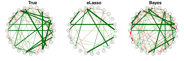
Figure 1: A single example data was simulated from probability mass function (8) with $\alpha=0$. The conditional independence graph was estimated under the correct assumption that $\alpha=0$. An edge between two distinct items $j$ and $k$ indicates that items $j$ and $k$ interact, that is, $\gamma_{j,k}\neq 0$. Green-colored edges represent positive interactions ($\gamma_{j,k}>0$), whereas red-colored edges represent negative interactions ($\gamma_{j,k}<0$). The width of an edge between two distinct items $j$ and $k$ is proportional to the strength of the interaction in terms of $|\gamma_{j,k}|$.

4.2 Simulation study with incorrect model specification: omitted covariate

In the second simulation study, we generate 500 data sets from probability mass function (8) with $\alpha=1/2$ and estimate the conditional independence graph of the generalized Ising model by eLasso and the Bayesian approach under the incorrect assumption that $\alpha=0$ (as described above). In other words, we estimate the conditional independence graph under an incorrect model specification.

To assess how well the Bayesian approach can recover the conditional independence graph compared with eLasso when the model is misspecified, we report the true-positive rate (TPR), the true-negative rate (TNR), and the Rand index in Table 2, averaged over the 500 simulated data sets.

	eLasso	Bayes
True-positive rate (TPR)	.206	.738
True-negative rate (TNR)	.997	.786
Rand index	.799	.774

Table 2: 500 data sets were simulated from probability mass function (8) with $\alpha=1/2$. The conditional independence graph was estimated under the incorrect assumption that $\alpha=0$. The performance of eLasso and the Bayesian approach is assessed in terms of the true-positive rate (TPR), the true-negative rate (TNR), and the Rand index, as defined in Equations (10), (11), and (12), respectively. These criteria are averaged over the 500 simulated data sets.

According to Table 2, the Bayesian approach is more robust against model misspecification due to omitted covariates than eLasso: The true-positive rate of eLasso drops from .227 (correct model specification, see Table 1) to .206 (incorrect model specification, see Table 2), which is a reduction of more than 9%. By contrast, the true-positive rate of the Bayesian approach drops from .752 (correct model specification, see Table 1) to .738 (incorrect model specification, see Table 2), which is a reduction of less than 2%. In other words, not only does the Bayesian approach appear to have a substantially higher true-positive rate than eLasso, but the true-positive rate of the Bayesian approach also appears to be less affected by model misspecification due to omitted covariates than the true-positive rate of eLasso.

Last, but not least, we simulate a single example data set from probability mass function (8) with $\alpha=1/2$ to gain more insight into how the Bayesian approach compares to eLasso in terms of graph recovery. Figure 2 compares the true conditional independence graph to the conditional independence graphs estimated by eLasso and the Bayesian approach and highlights the advantage of the Bayesian approach over eLasso when the model is misspecified: eLasso recovers 16 of the 69 edges in the true conditional independence graph, whereas the Bayesian approach recovers 52 of the 69 edges. Figure 3 compares the true interaction weights $\gamma_{j,k}$ and the estimated interaction weights $\widehat{\gamma}_{j,k}$, with the Bayesian approach outperforming eLasso. To quantify the advantage of the Bayesian approach over eLasso, we compute the root mean-squared error of the estimators of the true interaction weights $\gamma_{j,k}$:

$$\begin{array}[]{lllllllllllll}\mbox{RMSE}&=&\sqrt{\displaystyle\sum_{j<k}^{p}\,(\widehat{\gamma}_{j,k}-{\gamma}_{j,k})^{2}}.\end{array}$$

Here, $\widehat{\gamma}_{j,k}$ is the estimate of the data-generating interaction weight $\gamma_{j,k}$, which is either the $\ell_{1}$-penalized logistic regression estimate (eLasso) or the posterior mean provided $\gamma_{j,k}$ is estimated to be non-zero (Bayesian approach). It is worth noting that eLasso computes two estimates of $\gamma_{j,k}$: one estimate based on the $\ell_{1}$-penalized logistic regression of item response $X_{i,j}$ on $X_{i,k}$ and all other item responses, and one estimate based on the $\ell_{1}$-penalized logistic regression of item response $X_{i,k}$ on $X_{i,j}$ and all other item responses ($i=1,\dots,n$). These two estimates of $\gamma_{j,k}$ can differ. To report a single estimate of $\gamma_{j,k}$, eLasso averages over these two estimates, and we follow eLasso here. The RMSE of eLasso turns out to be 23.73, whereas the RMSE of the Bayesian approach is 13.64. By comparison, if the model specification is correct, the RMSE of eLasso and the Bayesian approach are 15.58 and 18.57, respectively. In other words, when the model specification is correct, eLasso may have a small advantage over the Bayesian approach, but when the model specification is incorrect, the Bayesian approach appears to outperform eLasso in terms of RMSE.

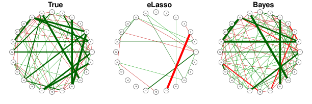
Figure 2: A single example data was simulated from probability mass function (8) with $\alpha=1/2$. The conditional independence graph was estimated under the incorrect assumption that $\alpha=0$. An edge between two distinct items $j$ and $k$ indicates that items $j$ and $k$ interact, that is, $\gamma_{j,k}\neq 0$. Green-colored edges represent positive interactions ($\gamma_{j,k}>0$), whereas red-colored edges represent negative interactions ($\gamma_{j,k}<0$). The width of an edge between two distinct items $j$ and $k$ is proportional to the strength of the interaction in terms of $|\gamma_{j,k}|$.

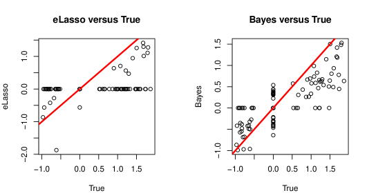
Figure 3: 500 data sets were simulated from probability mass function (8) with $\alpha=1/2$. The conditional independence graph was estimated under the incorrect assumption that $\alpha=0$. The estimated interaction weights $\widehat{\gamma}_{j,k}$ are plotted against the true interaction weights $\gamma_{j,k}$. The red-colored line is the identity line.

5 Applications to educational data

We compare the Bayesian approach to eLasso by using three educational data sets. In each application, we compare the conditional independence graphs estimated by eLasso and the Bayesian approach, and assess the goodness-of-fit of the estimated models. We first provide some background on how to assess goodness-of-fit in Section 5.1 and then present the three applications in Sections 5.2—5.4.

5.1 Goodness-of-fit statistics

To assess the goodness-of-fit (GOF) of the estimated models, we simulate 1,000 data sets from the estimated models.

In the case of eLasso, we simulate model-based predictions of item responses based on the estimates of the intercepts $\beta_{j}$ and the interaction weights $\gamma_{j,k}$ reported by eLasso. It is worth repeating that eLasso computes two estimates of $\gamma_{j,k}$: one estimate based on the $\ell_{1}$-penalized logistic regression of item response $X_{i,j}$ on $X_{i,k}$ and all other item responses, and one estimate based on the $\ell_{1}$-penalized logistic regression of item response $X_{i,k}$ on $X_{i,j}$ and all other item responses ($i=1,\dots,n$). To report a single estimate of $\gamma_{j,k}$, eLasso averages over these two estimates, and we follow eLasso here. In the case of the Bayesian approach, we generate posterior predictions.

We compare the simulated and observed data in terms of two statistics: (1) $\sum_{i=1}^{n}\,x_{i,j}$, which measures the easiness of item $j$ (intercept); and (2) $\sum_{i=1}^{n}x_{i,j}\,x_{i,k}$, which measures the strength of the interaction of two distinct items $j$ and $k$ (interactions). These two statistics are sufficient statistics for the intercepts $\beta_{j}$ and interaction weights $\gamma_{j,k}$. In addition, we assess the GOF of the estimated models in terms of higher-order statistics. To do so, we first compute, for each respondent $i$, an item-item graph where two distinct items $j$ and $k$ are connected by an edge if and only if respondent $i$ gave correct responses to both items $j$ and $k$. The item-item graphs of respondents should not be confused with the conditional independence graph of the Ising model: Item-item graphs represent data structure (the responses of respondents to pairs of items), whereas the conditional independence graph of the Ising model represents model structure (the conditional independence structure of the Ising model). We then compute the number of cliques of size $l$ in the item-item graph of each of the $n$ respondents, and average the number of cliques of size $l$ over the $n$ respondents. A clique of size $l$ is a maximal complete subset of nodes, that is, a subset of $l$ nodes such that all $\binom{l}{2}$ pairs of nodes are connected by edges and it is impossible to add nodes without losing the property of completeness (Lauritzen, 1996). These goodness-of-fit statistics are used in the three applications in Sections 5.2—5.4.

5.2 Abortion data

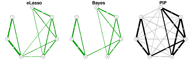
Figure 4: Abortion data: Conditional independence graphs estimated by eLasso and the Bayesian approach based on a Markov chain Monte Carlo sample of size 10,000. An edge between two distinct items $j$ and $k$ indicates that items $j$ and $k$ interact, that is, $\gamma_{j,k}\neq 0$. Green-colored edges represent positive interactions ($\gamma_{j,k}>0$), whereas red-colored edges represent negative interactions ($\gamma_{j,k}<0$). The width of an edge between two distinct items $j$ and $k$ is proportional to the strength of the interaction in terms of $|\gamma_{j,k}|$. The graph labeled PIP shows the posterior interaction probabilities of pairs of distinct items $j$ and $k$, that is, the posterior probability of the event that the indicator $\lambda_{i}$ corresponding to the interaction weight $\gamma_{j,k}$ equals $1$.

We first use a classic data set consisting of data on attitudes towards abortion, collected by the British Social Attitudes Survey Panel between 1983 and 1986 (Social and Community Planning Research, 1987). Respondents were asked whether abortion should be allowed by law under the following circumstances:

1. The woman decides on her own whether she does not wish to have the child.

2. The couple agrees that they do not wish to have the child.

3. The woman is not married and does not wish to marry the man.

4. The couple cannot afford any more children.

5. There is a strong chance of a defect in the baby.

6. The woman’s health is seriously endangered by the pregnancy.

7. The woman became pregnant as a result of rape.

The data correspond to binary responses (either 1=“yes” or 0=“no”) by $n=642$ individuals to the $p=7$ items described above. The resulting Ising model has $p+\binom{p}{2}=28$ parameters.

When applied to the abortion data, eLasso takes about 3/10 seconds, whereas the Bayesian approach takes about 5.4 minutes. Implementation details are provided in Sections 3.2 and 3.3.

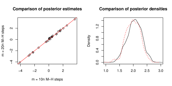
Figure 5: Abortion data. Left: posterior means of all $\theta_{i}$’s based on $m=10\,n$ and $m=20\,n$ Metropolis-Hastings (M-H) steps in Step 2 of Algorithm 1. Right: posterior density of $\gamma_{1,2}$. The solid and dotted lines indicate posterior densities obtained based on $m=10\,n$ and $m=20\,n$ Metropolis-Hastings (M-H) steps, respectively.

We first assess the performance of the Bayesian algorithm as a function of $m$ by running it with $m=10\,n$ and $m=20\,n$ in Step 2 of Algorithm 1. Figure 5 indicates that posterior means and posterior distributions do not change much as $m$ is increased.

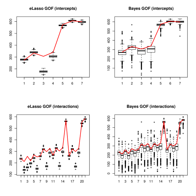
Figure 6: Abortion data: GOF assessment in terms of sufficient statistics for the intercepts $\beta_{j}$ and the interaction weights $\gamma_{j,k}$ based on 1,000 simulated data sets. The sufficient statistics are stated in Section 5.1. The red lines indicate the observed values of the sufficient statistics.

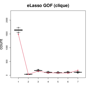
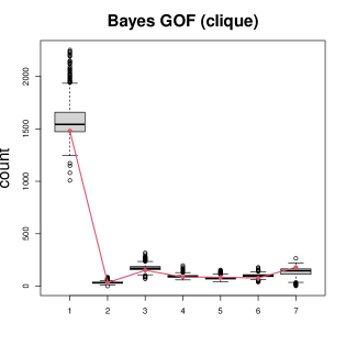
Figure 7: Abortion data: GOF assessment in terms of cliques based on 1,000 simulated data sets. For each simulated data set and each respondent, the number of cliques of size $l$ in the simulated item-item graph is computed, and then summed over all $n$ respondents. The red lines indicate the number of cliques of size $l$ in the observed item-item graphs, summed over the $n$ respondents.

The conditional independence graphs estimated by eLasso and the Bayesian approach are represented in Figure 4. To compare them, note that Jeon et al. (2021) detected two groups of items in the abortion data set by using latent space item response models: The first group of items (items 1–4) measures whether women may abort for personal reasons, whereas the second group of items (items 5–7) measures whether women may abort for medical or other reasons. According to Figure 4, both eLasso and the Bayesian approach agree with the observation of Jeon et al. (2021) that there are two groups of items with more connections within groups than between groups, but the Bayesian approach shows a more clear-cut separation of the two groups of items compared with eLasso. To shed light onto the difference between eLasso and the Bayesian approach, we inspect the posterior interaction probabilities of pairs of distinct items $j$ and $k$, that is, the posterior probability of the event that the indicator $\lambda_{i}$ corresponding to the interaction weight $\gamma_{j,k}$ equals $1$. Comparing the eLasso estimate of the conditional independence graph to the posterior interaction probabilities reveals that eLasso seems to connect all pairs of items with a posterior interaction probability of at least $.42$. By contrast, the Bayesian approach connects pairs of items with a posterior interaction probability of at least 1/2. In other words, it seems that eLasso is liberal compared with the Bayesian approach, at least if the two-group structure found by Jeon et al. (2021) is accepted as a reference point. It is worth pointing out that the true conditional independence graph is unknown, but the two-group structure found by Jeon et al. (2021) makes sense, because the first group of items is concerned with abortion for personal reasons, whereas the second group of items is concerned with abortion for medical and other reasons.

Last, but not least, we assess the GOF of the estimated models. Figure 6 suggests that the Bayesian approach outperforms eLasso in terms of sufficient statistics for the interaction weights $\gamma_{j,k}$. Figure 7 reveals that both the Bayesian approach and eLasso match the observed number of cliques rather well, although the Bayesian approach may have a small advantage over eLasso with respect to cliques of sizes 1 and 7. Here, as in Sections 5.3 and 5.4, there appears to be more variation in the model-based predictions of the Bayesian approach compared with eLasso. The reason is that the Bayesian approach takes into account the uncertainty about the parameters and averages over all parameters, whereas eLasso does not.

5.3 Deductive Reasoning Verbal (DRV) data

The Competence Profile Test of Deductive Reasoning Verbal (DRV: Spiel et al., 2001; Spiel and Gluck, 2008) was developed based on Piaget’s cognitive developmental theory (Piaget, 1971), with a view to evaluating the cognitive development stages of children and adolescents. The data set consists of $n=418$ respondents and $p=24$ items. Some information about the items of the DRV data set can be found in the supplement and more information can be found in Spiel et al. (2001) and Jin and Jeon (2019). The resulting Ising model has $p+\binom{p}{2}=300$ parameters.

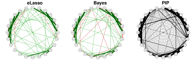
Figure 8: DRV data: estimated conditional independence graphs based on eLasso and the Bayesian approach with a Markov chain Monte Carlo sample of size 20,000. An edge between two distinct items $j$ and $k$ indicates that items $j$ and $k$ interact, that is, $\gamma_{j,k}\neq 0$. Green-colored edges represent positive interactions ($\gamma_{j,k}>0$), whereas red-colored edges represent negative interactions ($\gamma_{j,k}<0$). The width of an edge between two distinct items $j$ and $k$ is proportional to the strength of the interaction in terms of $|\gamma_{j,k}|$. The graph labeled PIP shows the posterior interaction probabilities of pairs of distinct items $j$ and $k$, that is, the posterior probability of the event that the indicator $\lambda_{i}$ corresponding to the interaction weight $\gamma_{j,k}$ equals $1$.

Applied to the DRV data set, eLasso approach takes about .94 seconds, whereas the Bayesian approach takes about 3.5 hours. To assess whether the number $m$ of Metropolis-Hastings steps in Step 2 of the Bayesian algorithm was large enough, we increase $m=10\,n$ to $m=20\,n$. Figure 9 suggests that the results do not change too much when $m$ is increased from $m=10\,n$ to $m=20\,n$. The estimated conditional independence graphs obtained by eLasso and the Bayesian approach are shown in Figure 8. eLasso and the Bayesian approach agree on the signs of 244 of the 276 interaction weights $\gamma_{j,k}$. The eLasso approach reports 209 edges, whereas the Bayesian approach reports 203 edges. The Bayesian approach reports more edges with negative interaction weights (22) than eLasso (8). Although the true conditional independence graph is unknown, it is known that some the items in the DRV test have a negative logical relationship by construction: e.g., items 7 and 8 have a negative logical relationship by construction, and both eLasso and the Bayesian approach report an edge with a negative interaction weight $\gamma_{7,8}$, but eLasso reports fewer other negative relationships than the Bayesian approach.

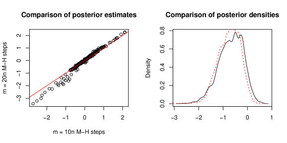
Figure 9: DRV data: Left: posterior means of all $\theta_{i}$’s based on $m=10\,n$ and $m=20\,n$ Metropolis-Hastings (M-H) steps in Step 2 of Algorithm 1. Right: posterior density of $\gamma_{1,2}$. The solid and dotted lines indicate posterior densities obtained based on $m=10\,n$ and $m=20\,n$ Metropolis-Hastings (M-H) steps, respectively.

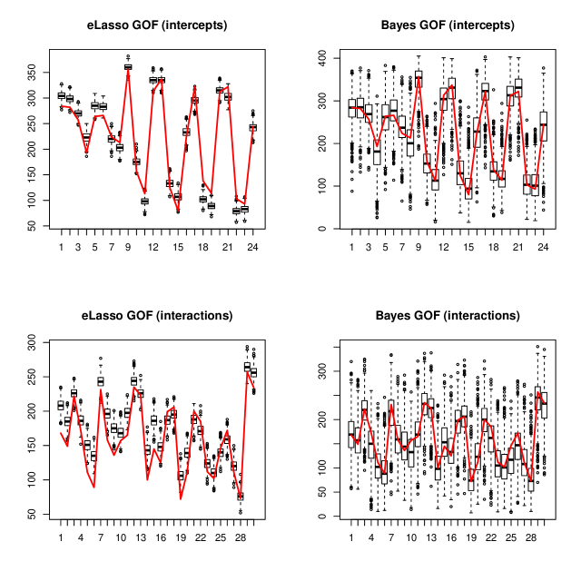
Figure 10: DRV data: GOF assessment in terms of sufficient statistics for the intercepts $\beta_{j}$ and the interaction weights $\gamma_{j,k}$ based on 1,000 simulated data sets. The sufficient statistics are stated in Section 5.1. The red lines indicate the observed values of the sufficient statistics.

As in the previous example, we assess the GOF of the estimated model. Since we have 300 sufficient statistics for 24 intercepts and 276 interactions, we show sufficient statistics for the intercept and first 30 interaction weights. Figures 10 and 11 suggest that the Bayesian approach compares favorably to eLasso in terms of GOF with respect to sufficient statistics for the intercepts $\beta_{j}$ and the interaction weights $\gamma_{j,k}$, and cliques.

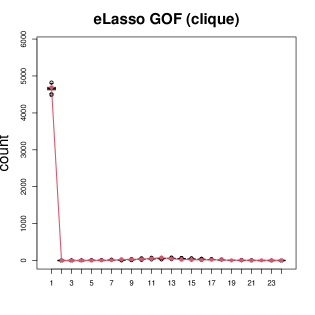
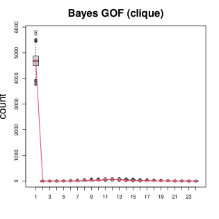
Figure 11: DRV data: GOF assessment in terms of cliques based on 1,000 simulated data sets. For each simulated data set and each respondent, the number of cliques of size $l$ in the simulated item-item graph is computed, and then summed over all $n$ respondents. The red lines indicate the number of cliques of size $l$ in the observed item-item graphs, summed over the $n$ respondents.

5.4 Korean middle school data

For decades, the Korean public K-12 system has been criticized for creating a competitive environment that may have a negative impact on the intellectual, mental, and behavioral development of students. To understand the developmental status of students and evaluate the effect of the competitive environment, the Office of Education in Gyeongi Province (the Seoul Metropolitan area) conducted surveys to assess the mental and physical health, creativity, ethics, autonomy, and democratic conciseness of students (Gyeonggi Provincial Office of Education, 2012). The data was collected in 2014 and concern 9th grade students (3rd grade students in the Korean middle school). All responses were transformed into binary responses: 1 (“strongly disagree”), 2 (“disagree”), and 3 (“do not disagree or agree”) were transformed to 0; and 4 (“agree”) and 5 (“strongly agree”) were transformed to 1. We analyze the middle school data set consisting of $n=$ 3,784 respondents and $p=70$ items. A list of all items can be found in the supplement. The resulting Ising model has $p+\binom{p}{2}=$ 2,485 parameters.

The Bayesian approach takes about 430 hours, whereas the eLasso approach takes about 24.33 seconds. The eLasso approach sets 2,101 of the 2,415 interaction weights $\gamma_{j,k}$ to 0. By contrast, the Bayesian approach sets 1,992 of the interaction weights to 0. The eLasso approach and the Bayesian approach agree on the sign of 1,980 of the 2,415 interaction weights $\gamma_{j,k}$. The estimated conditional independence graphs are shown in Figure 12.

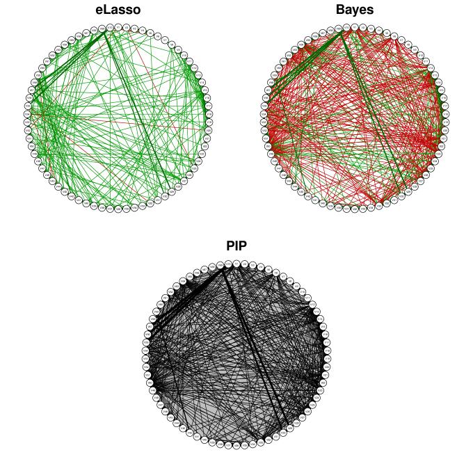
Figure 12: Korean middle school data: Conditional independence graphs estimated by eLasso and the Bayesian approach, based on a Markov chain Monte Carlo sample of size 20,000. An edge between two distinct items $j$ and $k$ indicates that items $j$ and $k$ interact, that is, $\gamma_{j,k}\neq 0$. Green-colored edges represent positive interactions ($\gamma_{j,k}>0$), whereas red-colored edges represent negative interactions ($\gamma_{j,k}<0$). The width of an edge between two distinct items $j$ and $k$ is proportional to the strength of the interaction in terms of $|\gamma_{j,k}|$. The graph labeled PIP shows the posterior interaction probabilities of pairs of distinct items $j$ and $k$, that is, the posterior probability of the event that the indicator $\lambda_{i}$ corresponding to the interaction weight $\gamma_{j,k}$ equals $1$.

Positive	Item name	Estimate
$\gamma_{29,30}$	“appearance satisfaction” (29), “appearance esteem” (30)	3.90
		(2.16, 5.58)
$\gamma_{4,5}$	“feel lonely” (4), “feel sad/depressed” (5)	3.68
		(1.81, 5.69)
$\gamma_{42,43}$	“nervous when take the exam” (42), “nervous before the exam” (43)	3.45
		(1.76, 5.05)
$\gamma_{23,26}$	“like to hang out with others” (23), “happy to be with someone else” (26)	3.20
		(1.10, 5.28)
$\gamma_{32,33}$	“ability does not change” (32), “even if I try, ability does not change” (33)	2.98
		(.50, 5.27)
Negative	Item name	Estimate
$\gamma_{6,70}$	“mental ill-being” (6), “self-esteem” (70)	-.55
		(-2.72, 1.13)
$\gamma_{49,62}$	“relationship with friends” (49), “academic stress” (62)	-.50
		(-2.65, 1.15)
$\gamma_{12,64}$	“sense of citizenship” (12), “academic stress” (64)	-.50
		(-2.57, 1.31)
$\gamma_{12,61}$	“sense of citizenship” (12), “academic stress” (61)	-.486
		(-2.61, 1.25)
$\gamma_{37,50}$	“self-driven learning” (37), “relationship with friends” (50)	-.46
		(-2.46, 1.50)

Table 3: Korean middle school data: the five strongest positive and negative interactions in terms of the posterior mean of the interaction weights $\gamma_{j,k}$. The estimates mentioned above are posterior means. The intervals are 95% posterior credible intervals.

We provide some descriptive explanations based on the top 5 strongest positive and negative interactions in terms of the posterior mean of the parameters $\gamma_{j,k}$ shown in Table 3. To interpret the results, we present unofficial translations of the Korean items within quotation marks. The strongest positive interaction occurs between items 29 (“I have a favorable face”) and 30 (”My appearance is attractive”), which may be unsurprising. The second strongest positive interaction occurs between items 4 (“Sometimes I experience loneliness for no reason”) and 5 (“At times I am sad and depressed for no reason”), suggesting that loneliness is related to sadness. The third strongest positive interaction occurs between items 42 (“I am nervous when I try to take the exam”) and 43 (“I am more nervous before the exam”). Both items measure test anxiety.

The strongest negative interaction occurs between items 6 (“I sometimes want to die for no reason”) and 70 (“I have a positive attitude towards myself”), which makes sense, because the two questions measure opposite attitudes. The second strongest negative interaction occurs between items 49 (“I feel comfortable when I am with my school friends”) and 62 (“I feel uneasy when I play with my friends”), which likewise measure opposite attitudes. The third strongest negative interaction occurs between items 12 (“Foreigners living in Korea should be treated in the same way as Koreans”) and 64 (“I can ignore friendship to get better grades in grade or entrance exams”), suggesting a negative association between compassion for foreigners and selfish pursuit of academic interests.

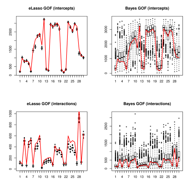
Figure 13: Korean middle school data. GOF assessment in terms of sufficient statistics for the intercepts $\beta_{j}$ and the interaction weights $\gamma_{j,k}$ based on 1,000 simulated data sets. The red lines indicate the observed values of the sufficient statistics.

Last, but not least, we assess the GOF of the estimated models. The figure shows the GOF of the estimated models in terms of the sufficient statistics for the first 30 intercepts and interaction weights—note that there are 2,480 parameters and hence 2,480 sufficient statistics, and displaying the GOF of the estimated models in terms of all 2,480 sufficient statistics is too space-consuming. Figures 13 and 14 indicate that the Bayesian approach performs well in terms of GOF compared with eLasso. As before, there appears to be more variation in the model-based predictions of the Bayesian approach compared with eLasso, arising from the fact that the posterior predictions take into account the uncertainty about the parameters, whereas the model-based predictions of eLasso do not.

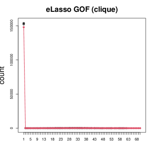
Figure 14: Korean middle school data: GOF assessment in terms of cliques, averaged over the $n$ item-item repondent networks of the $n$ respondents. The red lines indicate the observed numbers of cliques, summed over the $n$ item-item repondent networks of the $n$ respondents.

6 Discussion

We have developed a Bayesian approach for Ising models with doubly-intractable posterior distributions, with applications to educational data. The proposed approach helps quantify the uncertainty about the estimated conditional independence graph along with the parameters of the model, and appears to be more robust against model misspecification due to omitted covariates than the $\ell_{1}$-penalized nodewise logistic regression approach.

To address the statistical and computational challenges arising from doubly-intractable posterior distributions, we have combined two approaches: (1) a double Metropolis-Hastings algorithm algorithm (Liang, 2010) and (2) stochastic search variable selection methods (George and McCulloch, 1993; Ishwaran and Rao, 2005). We note that the proposed Bayesian approach is inexact, in the sense that the stationary distribution of the Markov chains constructed by the proposed Bayesian algorithm is not the desired target posterior. The reason is that the double Metropolis-Hastings algorithm algorithm generates an auxiliary variable from an approximate distribution in Step 2 of Algorithm 1 on page 1. However, the double Metropolis-Hastings algorithm is feasible in high-dimensional settings with thousands of parameters, whereas many alternatives are not. Several approaches have been developed to reduce variance, but are inexact. For example, Alquier et al. (2016) and Stoehr et al. (2017) provide Hamiltonian variants of double Metropolis-Hastings algorithm, and Friel et al. (2016) develops control variates for intractable likelihood functions. Developing an exact algorithm for such models is still an open question (leaving aside perfect sampling, which can be expensive in terms of computing time)

It is worth noting that there variations on the approach proposed here, depending on the choice of the variable selection method (see, e.g., O’Hara et al., 2009). For instance, instead of using the vector of indicators $\bm{\lambda}$ in the model, Bayesian lasso methods (Park and Casella, 2008; Yi and Xu, 2008) directly approximate the spike and slab shape of the prior on the model parameters $\bm{\theta}$. The horseshoe prior (Carvalho et al., 2010) is a promising alternative.

An open issue is the scalability of the Bayesian algorithm, that is, the ability of the Bayesian algorithm to scale up to larger data sets with more respondents $n$ or more items $p$. While we were able to apply the Bayesian algorithm to Ising models with $p+\binom{p}{2}=$ 2,485 parameters based on item responses from $n=$ 3,784 respondents (Section 5.4), the computing time required to obtain samples from an approximation to the posterior distribution (430 hours, that is, almost 18 days) suggests that more work is needed to scale up the Bayesian algorithm to larger $n$ and larger $p$. One of the main computational bottlenecks is the generation of auxiliary variables. There are a number of ideas for addressing these computational challenges. For instance, Park and Haran (2020) propose a function emulation approach that replaces expensive importance sampling schemes with fast Gaussian process approximations. Bouranis et al. (2017) provides a practical Bayesian approach for large networks by correcting Markov chain Monte Carlo samples from pseudo-posterior distribution. These and other ideas—and combinations of them—constitute interesting avenues for future research.

Supplementary materials

The supplement provides more background on the data sets used in Section 5. All data and all source code used in the paper can be downloaded from https://github.com/jwpark88/itemBayes.

References

- Agresti (2002) Agresti, A. (2002). Categorical Data Analysis (2 ed.). Hoboken: John Wiley & Sons.
- Alquier et al. (2016) Alquier, P., N. Friel, R. Everitt, and A. Boland (2016). Noisy Monte Carlo: Convergence of Markov chains with approximate transition kernels. Statistics and Computing 26(1-2), 29–47.
- Anandkumar et al. (2012) Anandkumar, A., V. Y. F. Tan, F. Huang, and A. S. Willsky (2012). High-dimensional structure estimation in Ising models: Local separation criterion. The Annals of Statistics 40, 1346–1375.
- Atchadé (2006) Atchadé, Y. F. (2006). An adaptive version for the Metropolis adjusted Langevin algorithm with a truncated drift. Methodology and Computing in Applied Probability 8(2), 235–254.
- Atchade et al. (2013) Atchade, Y. F., N. Lartillot, and C. Robert (2013). Bayesian computation for statistical models with intractable normalizing constants. Brazilian Journal of Probability and Statistics 27(4), 416–436.
- Beaumont et al. (2002) Beaumont, M. A., W. Zhang, and D. J. Balding (2002). Approximate Bayesian computation in population genetics. Genetics 162(4), 2025–2035.
- Besag (1974) Besag, J. (1974). Spatial interaction and the statistical analysis of lattice systems. Journal of the Royal Statistical Society. Series B (Methodological) 36, 192–236.
- Besag (1974) Besag, J. (1974). Spatial interaction and the statistical analysis of lattice systems. Journal of the Royal Statistical Society, Series B 36, 192–225.
- Borsboom (2008) Borsboom, D. (2008). Psychometric perspectives on diagnostic systems. Journal of Clinical Psychology 64(9), 1089–1108.
- Bouranis et al. (2017) Bouranis, L., N. Friel, and F. Maire (2017). Efficient Bayesian inference for exponential random graph models by correcting the pseudo-posterior distribution. Social Networks 50, 98–108.
- Bouranis et al. (2018) Bouranis, L., N. Friel, and F. Maire (2018). Bayesian model selection for exponential random graph models via adjusted pseudolikelihoods. Journal of Computational and Graphical Statistics 27(3), 516–528.
- Bresler and Karzand (2020) Bresler, G. and M. Karzand (2020). Learning a tree-structured Ising model in order to make predictions. The Annals of Statistics 48, 713–737.
- Bühlmann and van de Geer (2011) Bühlmann, P. and S. van de Geer (2011). Statistics for High-Dimensional Data: Methods, Theory and Applications. New York: Springer-Verlag.
- Butts (2018) Butts, C. T. (2018). A perfect sampling method for exponential family random graph models. The Journal of Mathematical Sociology 42(1), 17–36.
- Caimo and Friel (2011) Caimo, A. and N. Friel (2011). Bayesian inference for exponential random graph models. Social Networks 33(1), 41–55.
- Caimo and Friel (2013) Caimo, A. and N. Friel (2013). Bayesian model selection for exponential random graph models. Social Networks 35(1), 11–24.
- Caimo and Friel (2014) Caimo, A. and N. Friel (2014). Bergm: Bayesian Exponential Random Graphs in R. Journal of Statistical Software 61, 1–25.
- Caimo and Gollini (2020) Caimo, A. and I. Gollini (2020). A multilayer exponential random graph modelling approach for weighted networks. Computational Statistics & Data Analysis 142, 106–125.
- Carvalho et al. (2010) Carvalho, C. M., N. G. Polson, and J. G. Scott (2010). The horseshoe estimator for sparse signals. Biometrika 97(2), 465–480.
- Chatterjee (2007) Chatterjee, S. (2007). Stein’s method for concentration inequalities. Probability Theory and Related Fields 138, 305–321.
- Chen and Chen (2008) Chen, J. and Z. Chen (2008). Extended Bayesian information criteria for model selection with large model spaces. Biometrika 95, 759–771.
- Eddelbuettel et al. (2011) Eddelbuettel, D., R. François, J. Allaire, J. Chambers, D. Bates, and K. Ushey (2011). Rcpp: Seamless R and C++ integration. Journal of Statistical Software 40(8), 1–18.
- Epskamp et al. (2018) Epskamp, S., D. Borsboom, and E. I. Fried (2018). Estimating psychological networks and their accuracy: A tutorial paper. Behavior Research Methods 50, 195–212.
- Everitt (2012) Everitt, R. G. (2012). Bayesian parameter estimation for latent Markov random fields and social networks. Journal of Computational and Graphical Statistics 21, 940–960.
- Flegal et al. (2008) Flegal, J. M., M. Haran, and G. L. Jones (2008). Markov chain Monte carlo: Can we trust the third significant figure? Statistical Science 23, 250–260.
- Frank and Strauss (1986) Frank, O. and D. Strauss (1986). Markov graphs. Journal of the American Statistical Association 81, 832–842.
- Friel et al. (2016) Friel, N., A. Mira, C. J. Oates, et al. (2016). Exploiting multi-core architectures for reduced-variance estimation with intractable likelihoods. Bayesian Analysis 11(1), 215–245.
- George and McCulloch (1993) George, E. and R. McCulloch (1993). Variable selection via Gibbs sampling. Journal of the American Statistical Association 88, 881–889.
- Ghosal and Mukherjee (2020) Ghosal, P. and S. Mukherjee (2020). Joint estimation of parameters in Ising model. The Annals of Statistics 48, 785–810.
- Goldstein (2015) Goldstein, J. (2015). Compartmental, spatial and point process models for infectious diseases. Ph. D. thesis, the Pennsylvania State University.
- Gyeonggi Provincial Office of Education (2012) Gyeonggi Provincial Office of Education (2012). Plan of innovation school management. Republic of Korea: Gyeonggi Province.
- Hunter and Handcock (2012) Hunter, D. R. and M. S. Handcock (2012). Inference in curved exponential family models for networks. Journal of Computational and Graphical Statistics.
- Hunter et al. (2012) Hunter, D. R., P. N. Krivitsky, and M. Schweinberger (2012). Computational statistical methods for social network models. Journal of Computational and Graphical Statistics 21, 856–882.
- Ishwaran and Rao (2005) Ishwaran, H. and J. S. Rao (2005). Spike and slab variable selection: Frequentist and Bayesian strategies. The Annals of Statistics 33, 730–773.
- Ising (1925) Ising, E. (1925). Beitrag zur Theorie des Ferromagnetismus. Zeitschrift für Physik A 31, 253–258.
- Jeon et al. (2021) Jeon, M., I. H. Jin, M. Schweinberger, and S. Baugh (2021). Mapping unobserved item-respondent interactions: A latent space item response model with interaction map. Psychometrika. To appear.
- Jin and Jeon (2019) Jin, I. H. and M. Jeon (2019). A doubly latent space joint model for local item and person dependence in the analysis of item response data. Psychometrika 84(1), 236–260.
- Jin et al. (2013) Jin, I. H., Y. Yuan, and F. Liang (2013). Bayesian analysis for exponential random graph models using the adaptive exchange sampler. Statistics and its Interface 6, 559–576.
- Jones et al. (2006) Jones, G. L., M. Haran, B. S. Caffo, and R. Neath (2006). Fixed-width output analysis for Markov chain Monte Carlo. Journal of the American Statistical Association 101(476), 1537–1547.
- Koskinen (2004) Koskinen, J. (2004). Essays on Bayesian Inference for Social Networks. Ph. D. thesis, Stockholm University, Dept. of Statistics, Sweden.
- Koskinen et al. (2010) Koskinen, J. H., G. L. Robins, and P. E. Pattison (2010). Analysing exponential random graph (p-star) models with missing data using Bayesian data augmentation. Statistical Methodology 7, 366–384.
- Lauritzen (1996) Lauritzen, S. (1996). Graphical Models. Oxford, UK: Oxford University Press.
- Lederer (2021) Lederer, J. (2021). Fundamentals of High-Dimensional Statistics—With Exercises and R Labs. Springer Texts in Statistics. Heidelberg: Springer.
- Liang (2010) Liang, F. (2010). A double Metropolis–Hastings sampler for spatial models with intractable normalizing constants. Journal of Statistical Computation and Simulation 80(9), 1007–1022.
- Liang and Jin (2013) Liang, F. and I. H. Jin (2013). A Monte Carlo Metropolis-Hastings algorithm for sampling from distributions with intractable normalizing constants. Neural Computation 25(8), 2199–2234.
- Liang et al. (2016) Liang, F., I. H. Jin, Q. Song, and J. S. Liu (2016). An adaptive exchange algorithm for sampling from distributions with intractable normalizing constants. Journal of the American Statistical Association 111, 377–393.
- Lusher et al. (2013) Lusher, D., J. Koskinen, and G. Robins (2013). Exponential Random Graph Models for Social Networks. Cambridge, UK: Cambridge University Press.
- Lyne et al. (2015) Lyne, A., M. Girolami, Y. Atchade, H. Strathmann, and D. Simpson (2015). On Russian roulette estimates for Bayesian inference with doubly-intractable likelihoods. Statistical Science 30, 1–26.
- Maathuis et al. (2019) Maathuis, M., M. Drton, S. Lauritzen, and M. Wainwright (2019). Handbook of Graphical Models. Boca Raton, Florida: CRC Press.
- Marin et al. (2012) Marin, J. M., P. Pudlo, C. P. Robert, and R. J. Ryder (2012). Approximate Bayesian computational methods. Statistics and Computing 22(6), 1167–1180.
- Marjoram et al. (2003) Marjoram, P., J. Molitor, V. Plagnol, and S. Tavare (2003). Markov chain Monte Carlo without likelihoods. Proceedings of the National Academices of Science, USA 100, 15324–15328.
- Marsman et al. (2018) Marsman, M., D. Borsboom, J. Kruis, S. Epskamp, R. van Bork, L. J. Waldorp, H. L. J. van der Maas, and G. K. J. Maris (2018). An introduction to network psychometrics: Relating ising network models to item response theory models. Multivariate Behavioral Research 53, 15–35.
- Meinshausen and Bühlmann (2006) Meinshausen, N. and P. Bühlmann (2006). High-dimensional graphs and variable selection with the LASSO. The Annals of Statistics 34, 1436–1462.
- Møller et al. (2006) Møller, J., A. N. Pettitt, R. Reeves, and K. K. Berthelsen (2006). An efficient Markov chain Monte Carlo method for distributions with intractable normalising constants. Biometrika 93(2), 451–458.
- Murray et al. (2006) Murray, I., Z. Ghahramani, and D. J. C. MacKay (2006). MCMC for doubly-intractable distributions. In Proceedings of the 22nd Annual Conference on Uncertainty in Artificial Intelligence, pp. 359–366. Corvallis: AUAI Press.
- O’Hara et al. (2009) O’Hara, R. B., M. J. Sillanpää, et al. (2009). A review of Bayesian variable selection methods: what, how and which. Bayesian analysis 4(1), 85–117.
- Park and Haran (2018) Park, J. and M. Haran (2018). Bayesian inference in the presence of intractable normalizing functions. Journal of the American Statistical Association 113(523), 1372–1390.
- Park and Haran (2020) Park, J. and M. Haran (2020). A function emulation approach for doubly intractable distributions. Journal of Computational and Graphical Statistics 29(1), 66–77.
- Park and Casella (2008) Park, T. and G. Casella (2008). The Bayesian lasso. Journal of the American Statistical Association 103(482), 681–686.
- Piaget (1971) Piaget, J. (1971). Biology and knowledge. University of Chicago Press: Chicago.
- Pritchard et al. (1999) Pritchard, J., M. T. Seielstad, A. Perez-Lezaun, and M. W. Feldman (1999). Population growth of human Y chromosomes: A study of Y chromosome microsatellites. Molecular Biology and Evolution 16, 1791–1798.
- Propp and Wilson (1996) Propp, J. G. and D. B. Wilson (1996). Exact sampling with coupled Markov chains and applications to statistical mechanics. Random structures and Algorithms 9(1-2), 223–252.
- Rand (1971) Rand, W. M. (1971). Objective criteria for the evaluation of clustering methods. Journal of the American Statistical Association 66, 846–850.
- Ravikumar et al. (2010) Ravikumar, P., M. J. Wainwright, and J. Lafferty (2010). High-dimensional Ising model selection using -regularized logistic regression. The Annals of Statistics 38, 1287–1319.
- Robert et al. (2011) Robert, C. P., J. M. Cornuet, J. M. Marin, and N. S. Pillai (2011). Lack of confidence in approximate Bayesian computation model choice. Proceedings of the National Academy of Sciences 108(37), 15112–15117.
- Robins et al. (2007) Robins, G., P. Pattison, Y. Kalish, and D. Lusher (2007). An introduction to exponential random graph (p*) models for social networks. Social Networks 29(2), 173–191.
- Schweinberger and Handcock (2015) Schweinberger, M. and M. S. Handcock (2015). Local dependence in random graph models: characterization, properties and statistical inference. Journal of the Royal Statistical Society, Series B 77, 647–676.
- Schweinberger et al. (2020) Schweinberger, M., P. N. Krivitsky, C. T. Butts, and J. R. Stewart (2020). Exponential-family models of random graphs: Inference in finite, super, and infinite population scenarios. Statistical Science 35, 627–662.
- Shao (2003) Shao, J. (2003). Mathematical statistics (2 ed.). New York: Springer.
- Sisson et al. (2007) Sisson, S. A., Y. Fan, and M. M. Tanaka (2007). Sequential Monte Carlo without likelihoods. Proceedings of the National Academy of Sciences 104, 1760–1765.
- Social and Community Planning Research (1987) Social and Community Planning Research (1987). British Social Attitude, the 1987 Report. Gower Publishing.
- Spiel and Gluck (2008) Spiel, C. and J. Gluck (2008). A model based test of competence profile and competence level in deductive reasoning. In J. Hartig, E. Klieme, and D. Leutner (Eds.), Assessment of competencies in educational contexts: State of the art and future prospects, pp. 41–60. Gottingen: Hogrefe.
- Spiel et al. (2001) Spiel, C., J. Gluck, and H. Gossler (2001). Stability and change of unidimensionality: The sample case of deductive reasoning. Journal of Adolescent Research 16, 150–168.
- Stewart et al. (2019) Stewart, J. R., M. Schweinberger, M. Bojanowski, and M. Morris (2019). Multilevel network data facilitate statistical inference for curved ERGMs with geometrically weighted terms. Social Networks 59, 98–119.
- Stoehr et al. (2017) Stoehr, J., A. Benson, and N. Friel (2017). Noisy Hamiltonian Monte Carlo for doubly-intractable distributions. arXiv preprint arXiv:1706.10096.
- Strauss (1975) Strauss, D. J. (1975). A model for clustering. Biometrika 62(2), 467–475.
- Sundberg (2019) Sundberg, R. (2019). Statistical Modelling by Exponential Families. Cambridge, UK: Cambridge University Press.
- Thiemichen et al. (2016) Thiemichen, S., N. Friel, A. Caimo, and G. Kauermann (2016). Bayesian exponential random graph models with nodal random effects. Social Networks 46, 11–28.
- Toni et al. (2009) Toni, T., D. Welch, N. Strelkowa, A. Ipsen, and M. P. H. Stumpf (2009). Approximate Bayesian computation scheme for parameter inference and model selection in dynamical systems. Journal of the Royal Society Interface 6, 187–202.
- van Borkulo et al. (2016) van Borkulo, C., S. Epskamp, and A. Robitzsch (2016). IsingFit: Fitting Ising Models Using the ELasso Method. R package version 0.3.1.
- van Borkulo et al. (2014) van Borkulo, C. D., D. Borsboom, S. Epskamp, T. F. Blanken, L. Boschloo, R. A. Schoevers, and L. J. Waldorp (2014). A new method for constructing networks from binary data. Scientific Reports 4.
- Wainwright (2019) Wainwright, M. J. (2019). High-Dimensional Statistics. A Non-Asymptotic Viewpoint. Cambridge, UK: Cambridge University Press.
- Whittaker (2009) Whittaker, J. (2009). Graphical Models in Applied Multivariate Statistics. New York: John Wiley & Sons.
- Xue et al. (2012) Xue, L., H. Zou, and T. Cai (2012). Nonconcave penalized composite conditional likelihood estimation of sparse Ising models. The Annals of Statistics 40, 1403–1429.
- Yi and Xu (2008) Yi, N. and S. Xu (2008). Bayesian LASSO for quantitative trait loci mapping. Genetics 179(2), 1045–1055.
- Yin and Butts (2020) Yin, F. and C. T. Butts (2020). Kernel-based approximate Bayesian inference for Exponential Family Random Graph Models. arXiv:2004.08064.
- Zhao and Yu (2006) Zhao, P. and B. Yu (2006). On model selection consistency of the Lasso. Journal of Machine Learning Research 7, 2541–2563.