Graph Topological Aspects of Granger Causal Network Learning

Abstract

We study Granger causality in the context of wide-sense stationary time series, where our focus is on the topological aspects of the underlying causality graph. We establish sufficient conditions (in particular, we develop the notion of a “strongly causal” graph topology) under which the true causality graph can be recovered via pairwise causality testing alone, and provide examples from the gene regulatory network literature suggesting that our concept of a strongly causal graph may be applicable to this field. We implement and detail finite-sample heuristics derived from our theory, and establish through simulation the efficiency gains (both statistical and computational) which can be obtained (in comparison to LASSO-type algorithms) when structural assumptions are met.

Keywords— causality graph, Granger causality, network learning, time series, vector autoregression, LASSO

Acknowledgement

We acknowledge the support of the Natural Sciences and Engineering Research Council of Canada (NSERC), [funding reference number 518418-2018]. Cette recherche a été financée par le Conseil de recherches en sciences naturelles et en génie du Canada (CRSNG), [numéro de référence 518418-2018].

1 Introduction and Review

In this paper we study the notion of Granger causality [1] [2] as a means of uncovering an underlying causal structure in multivariate time series. Though the underlying causality graph cannot be observed directly, it’s presence is inferred as a latent structure among observed time series data. This notion is leveraged in a variety of applications e.g. in Neuroscience as a means of recovering interactions amongst brain regions [3], [4], [5]; in the study of the dependence and connectedness of financial institutions [6]; gene expression networks [7], [8], [9], [10]; and power system design [11], [12].

Granger causality can generally be formulated by searching for the “best” graph structure consistent with observed data, which is in general an extremely challenging problem (i.e. it may be framed as a best subset selection problem, see [13] for recent improvements in BSS methods), moreover, the comparison of quality between different structures, and hence the notion of “best” needs qualification. In applications where we are interested merely in minimizing the mean squared error of a linear one-step-ahead predictor, then we will be satisfied with an entirely dense graph of connections, since each edge can only serve to reduce estimation error. However, since the number of edges scales quadratically in $n$ (the number of nodes) it becomes imperative to infer a sparse causality graph for large systems, both to avoid overfitting observed data, as well as to aid the interpretability of the results.

A fairly early approach to the problem in the context of large systems is provided by [14], where the authors apply a local search heuristic to the Whittle likelihood with an AIC penalization. The local search heuristic is a common approach to combinatorial optimization due to it’s simplicity, but is liable to get stuck in shallow local minima.

A second and wildly successful heuristic is the LASSO regularizer [15], which can be understood as a natural convex relaxation to penalizing the count of the non-zero edges. The LASSO enjoys fairly strong theoretical guarantees [16], extending largely to the case of stationary time series data with a sufficiently fast rate of dependence decay [17] [18] [19], and variations on the LASSO have been applied in a number of different time series contexts as well as Granger causality [20] [21] [22] [23] [9]. One of the key improvements to the original LASSO algorithm is the adaptive (i.e. weighted) “adaLASSO” [24], for which oracle results (i.e. asymptotic support recovery) are established under less restrictive conditions than for the vanilla LASSO.

In the context of time series data, sparsity assumptions remain important, but there is significant additional structure that may arise as a result of considering the topology of the underlying Granger causality graph. The focus of this paper is to shed light on some of these topological questions, in particular, we study a particularly simple notion of graph topology which we term “strongly causal” and show that stationary times series whose underlying causality graph has this structure satisfy natural intuitive notions of “information flow” through the graph. Moreover, we show that such graphs are perfectly recoverable with only pairwise Granger causality tests, which would otherwise suffer from serious confounding problems (see [25] for earlier work on pairwise testing and [26] for earlier work on some of the problems considered here). Aside from being an interesting theoretical perspective, prior assumptions about the underlying graph (similarly to sparsity assumptions) can greatly improve upon the statistical power of causality graph recovery algorithms when the assumptions are met.

Detailed study of Granger causality for star structured graphs has been carried out in [27]. See as well [28], [29] for state space formulations.

In the case of gene expression networks, we show examples from the literature which suggest our concept of a “strongly causal graph” topology may have application in this field (see Section 2.5).

The principal contributions of this paper are as follows: firstly, in section 2 we study pairwise Granger causality relations, providing novel theorems connecting the structure of the causality graph to the pairwise “causality flow” in the system, as well as an interpretation in terms of the graph topology of the sparsity pattern of matrices arising in the Wold decomposition, generalizing in some sense the notion of “feedback-free” processes studied by [30] in close connection with Granger causality. We establish sufficient conditions (sections 2.5, 2.6) under which a fully conditional Granger causality graph can be recovered from pairwise tests alone (sec 2.7). We report a summary of simulation results in 3, with additional results reported in the supplementary material Section D. Our simulation results establish that there is significant potential for improvement over existing methods, and that the graph-topological aspects of time series analysis are relevant for both theory and practice. Concluding remarks on further open problems and extensions are provided in Section 4. The proofs of each proposition and theorem are also relegated to the supplementary material, simple corollaries have proofs included in the main text.

2 Graph Topological Aspects of Granger causality

2.1 Formal Setting

Consider the space $L_{2}(\Omega)$, the usual Hilbert space of finite variance random variables over a probability space $(\Omega,\mathcal{F},\mathbb{P})$ having inner product $\langle x,y\rangle=\mathbb{E}[xy]$. We will work with a discrete time and wide-sense stationary (WSS) $n$-dimensional vector valued process $x(t)$ (with $t\in\mathbb{Z}$) where the $n$ elements take values in $L_{2}$. We suppose that $x(t)$ has zero mean, $\mathbb{E}x(t)=0$, and has absolutely summable matrix valued covariance sequence $R(\tau)\overset{\Delta}{=}\mathbb{E}x(t)x(t-\tau)^{\mathsf{T}}$, and an absolutely continuous spectral density.

We will also work frequently with the spaces spanned by the values of such a process

$$\mathcal{H}_{t}^{(x)} =\mathsf{cl\ }\{\sum_{\tau=0}^{p}a_{\tau}^{\mathsf{T}}x(t-\tau)\ |\ a_{\tau}\in\mathbb{R}^{n},p\in\mathbb{N}\}\subseteq L_{2}(\Omega)$$ (1)

$$H_{t}^{(x)} =\{ax(t)\ |\ a\in\mathbb{R}\}\subseteq L_{2}(\Omega),$$

where the closure is naturally in mean-square. We will often omit the superscript $x$ which should be clear from context. Evidently these spaces are separable, and as closed subspaces of a Hilbert space they are themselves Hilbert. We will denote the spaces generated in analogous ways by particular components of $x$ as e.g. $\mathcal{H}_{t}^{(i,j)}$, $\mathcal{H}_{t}^{i}$ or by all but a particular component as $\mathcal{H}_{t}^{(-j)}$.

As a consequence of the Wold decomposition theorem (see e.g. [31]), every WSS sequence has the moving average $\mathsf{MA}(\infty)$ representation

$$x(t)=c(t)+\sum_{\tau=0}^{\infty}A(\tau)v(t-\tau),$$ (2)

where $c(t)$ is a purely deterministic sequence, $v(t)$ is an uncorrelated sequence and $A(0)=I$. We will assume that $c(t)=0$. Given our setup, this representation can be inverted to yield the $\mathsf{VAR}(\infty)$ form

$$x(t)=\sum_{\tau=1}^{\infty}B(\tau)x(t-\tau)+v(t).$$ (3)

The Equations (2), (3) can be represented as $x(t)=\mathsf{A}(z)v(t)=\mathsf{B}(z)x(t)+v(t)$ via the action (convolution) of the operators (LTI filters)

$$\mathsf{A}(z)\overset{\Delta}{=}\sum_{\tau=0}^{\infty}A(\tau)z^{-\tau}$$

and

$$\mathsf{B}(z)\overset{\Delta}{=}\sum_{\tau=1}^{\infty}B(\tau)z^{-\tau},$$

where the operator $z^{-1}$ is the back shift operator acting on $\ell_{2}^{n}(\Omega,\mathcal{F},\mathbb{P})$, that is:

$$\mathsf{B}_{ij}(z)x_{j}(t)\overset{\Delta}{=}\sum_{\tau=1}^{\infty}B_{ij}(\tau)x_{j}(t-\tau).$$ (4)

Finally, we have the inversion formula

$$\mathsf{A}(z)=(I-\mathsf{B}(z))^{-1}=\sum_{k=0}^{\infty}\mathsf{B}(z)^{k}.$$ (5)

The aforementioned assumptions are quite weak. The strongest assumption we require is finally that $\Sigma_{v}$ is a diagonal positive-definite matrix, which is referred to as a lack of instantaneous feedback in $x(t)$. We formally state our setup as a definition, which is the setup for the remainder of the paper:

Definition 1 (Basic Setup).

The process $x(t)$ is an $n$ dimensional wide sense stationary process having invertible $\mathsf{VAR}(\infty)$ representation (3) where $v(t)$ is sequentially uncorrelated and has a diagonal positive-definite covariance matrix. The $\mathsf{MA}(\infty)$ representation of Equation (2) has $c(t)=0$ and $A(0)=I$.

2.2 Granger Causality

Definition 2 (Granger Causality).

For the WSS series $x(t)$ satisfying the assumptions of Definition 1 we will say that component $x_{j}$ Granger-Causes (GC) component $x_{i}$ (with respect to $x$) and write $x_{j}\overset{\text{GC}}{\rightarrow}x_{i}$ if

$$\xi[x_{i}(t)\ |\ \mathcal{H}_{t-1}]<\xi[x_{i}(t)\ |\ \mathcal{H}^{(-j)}_{t-1}],$$ (6)

where $\xi[x\ |\ \mathcal{H}]\overset{\Delta}{=}\mathbb{E}(x-\hat{\mathbb{E}}[x\ |\ \mathcal{H}])^{2}$ is the mean squared estimation error and $\hat{\mathbb{E}}[x\ |\ \mathcal{H}]\overset{\Delta}{=}\text{proj}_{\mathcal{H}}(x)$ denotes the (unique) projection onto the Hilbert space $\mathcal{H}$.

This notion captures the idea that the process $x_{j}$ provides information about $x_{i}$ that is not available from elsewhere. The caveat “with respect to $x$” is important in that GC relations can change when components are added to or removed from our collection $x$ of observations, e.g. new GC relations can arise if we remove the observations of a common cause, and existing GC relations can disappear if we observe a new mediating series. The notion is closely related to the information theoretic measure of transfer entropy, indeed, if the distribution of $v(t)$ is known to be Gaussian then they are equivalent [32].

The notion of conditional orthogonality is the essence of Granger causality, and enables us to obtain results for a fairly general class of WSS processes, rather than simply $\mathsf{VAR}(p)$ models.

Definition 3 (Conditional Orthogonality).

Consider three closed subspaces of a Hilbert space $\mathcal{A}$, $\mathcal{B}$, $\mathcal{X}$. We say that $\mathcal{A}$ is conditionally orthogonal to $\mathcal{B}$ given $\mathcal{X}$ and write $\mathcal{A}\perp\mathcal{B}\ |\ \mathcal{X}$ if

$$\langle a-\hat{\mathbb{E}}[a\ |\ \mathcal{X}],b-\hat{\mathbb{E}}[b\ |\ \mathcal{X}]\rangle=0\ \forall a\in\mathcal{A},b\in\mathcal{B}.$$

An equivalent condition is that (see [31] Proposition 2.4.2)

$$\hat{\mathbb{E}}[\beta\ |\ \mathcal{A}\vee\mathcal{X}]=\hat{\mathbb{E}}[\beta\ |\ \mathcal{X}]\ \forall\beta\in\mathcal{B}$$

Theorem 1 (Granger Causality Equivalences).

The following are equivalent:

1. $x_{j}\overset{\text{GC}}{\nrightarrow}x_{i}$

2. $\forall\tau\in\mathbb{N}_{+}\ B_{ij}(\tau)=0$ i.e. $\mathsf{B}_{ij}(z)=0$

3. $H_{t}^{i}\perp\mathcal{H}_{t-1}^{(j)}\ |\ \mathcal{H}_{t-1}^{(-j)}$

4. $\hat{\mathbb{E}}[x_{i}(t)\ |\ \mathcal{H}_{t-1}^{(-j)}]=\hat{\mathbb{E}}[x_{i}(t)\ |\ \mathcal{H}_{t-1}]$

2.3 Granger Causality Graphs

We establish some graph theoretic notation and terminology, collected formally in definitions for the reader’s convenient reference.

Definition 4 (Graph Theory Review).

A graph $\mathcal{G}=(V,\mathcal{E})$ is simply a tuple of sets respectively called nodes and edges. Throughout this paper, we have in all cases $V=[n]\overset{\Delta}{=}\{1,2,\ldots,n\}$. We will also focus solely on directed graphs, where the edges $\mathcal{E}\subseteq V\times V$ are ordered pairs.

A (directed) path (of length $r$) from node $i$ to node $j$, denoted $i\rightarrow\cdots\rightarrow j$, is a sequence $a_{0},a_{1},\ldots,a_{r-1},a_{r}$ with $a_{0}=i$ and $a_{r}=j$ such that $\forall\ 0\leq k\leq r\ (a_{k},a_{k+1})\in\mathcal{E}$, and where $(a_{k},a_{k-1})$ are distinct for $0\leq k<r$.

A cycle is a path of length $2$ or more between a node and itself. An edge between a node and itself $(i,i)\in\mathcal{E}$ (which we do not consider to be a cycle) is referred to as a loop.

A graph $\mathcal{G}$ is a directed acyclic graph (DAG) if it is a directed graph and does not contain any cycles.

Definition 5 (Parents, Grandparents, Ancestors).

A node $j$ is a parent of node $i$ if $(j,i)\in\mathcal{E}$. The set of all $i$’s parents will be denoted $pa(i)$, and we explicitly exclude loops as a special case, that is, $i\not\in pa(i)$ even if $(i,i)\in\mathcal{E}$.

The set of level $\ell$ grandparents of node $i$, denoted $gp_{\ell}(i)$, is the set such that $j\in gp_{\ell}(i)$ if and only if there is a directed path of length $\ell$ in $\mathcal{G}$ from $j$ to $i$. Clearly, $pa(i)=gp_{1}(i)$.

Finally, the set of level $\ell$ ancestors of $i$: $\mathcal{A}_{\ell}(i)=\bigcup_{\lambda\leq\ell}gp_{\lambda}(i)$ is the set such that $j\in\mathcal{A}_{\ell}(i)$ if and only if there is a directed path of length $\ell$ or less in $\mathcal{G}$ from $j$ to $i$. The set of all ancestors of $i$ (i.e. $\mathcal{A}_{n}(i)$) is denoted simply $\mathcal{A}(i)$.

Recall that we do not allow a node to be it’s own parent, although unless $\mathcal{G}$ is a DAG, a node can be it’s own ancestor. We will occasionally need to explicitly exclude $i$ from $\mathcal{A}(i)$, in which case we will write $\mathcal{A}(i)\setminus\{i\}$.

Our principal object of study will be a graph determined by Granger causality relations as follows.

Definition 6 (Causality graph).

We define the Granger causality graph $\mathcal{G}=([n],\mathcal{E})$ to be the directed graph formed on $n$ vertices where an edge $(j,i)\in\mathcal{E}$ if and only if $x_{j}$ Granger-causes $x_{i}$ (with respect to $x$). That is,

$$(j,i)\in\mathcal{E}\iff j\in pa(i)\iff x_{j}\overset{\text{GC}}{\rightarrow}x_{i}.$$

The edges of the Granger causality graph $\mathcal{G}$ can be given a general notion of “weight” by associating an edge $(j,i)$ with the strictly causal LTI filter $\mathsf{B}_{ij}(z)$ (see Equation (4)). Thence, the matrix $\mathsf{B}(z)$ is analogous to a weighted adjacency matrix for the graph $\mathcal{G}$. And, in the same way that the $k^{\text{th}}$ power of an adjacency matrix counts the number of paths of length $k$ between nodes, $(\mathsf{B}(z)^{k})_{ij}$ is a filter isolating the “action” of $j$ on $i$ at a time lag of $k$ steps, this is exemplified in the inversion formula (5).

From the $\mathsf{VAR}$ representation of $x(t)$ there is clearly a tight relationship between each node and it’s parent nodes, the relationship is quantified through the sparsity pattern of $B(z)$. Similarly, the following proposition is analogous to the definition of feedback free processes of [30] and provides an interpretation of the sparsity pattern of $A(z)$ (from the MA representation of $x(t)$) in terms of the causality graph $\mathcal{G}$.

Proposition 1 (Ancestor Expansion).

The component $x_{i}(t)$ of $x(t)$ can be represented in terms of it’s parents in $\mathcal{G}$:

$$x_{i}(t)=v_{i}(t)+\mathsf{B}_{ii}(z)x_{i}(t)+\sum_{k\in pa(i)}\mathsf{B}_{ik}(z)x_{k}(t).$$ (7)

Moreover, $x_{i}$ can be expanded in terms of it’s ancestor’s $v(t)$ components only:

$$x_{i}(t)=\mathsf{A}_{ii}(z)v_{i}(t)+\sum_{\begin{subarray}{c}k\in\mathcal{A}(i)\\ k\neq i\end{subarray}}\mathsf{A}_{ik}(z)v_{k}(t),$$ (8)

where $\mathsf{A}(z)=\sum_{\tau=0}^{\infty}A(\tau)z^{-\tau}$ is the filter from the Wold decomposition representation of $x(t)$, Equation (2).

This statement is ultimately about the sparsity pattern in the Wold decomposition matrices $A(\tau)$ since $x_{i}(t)=\sum_{\tau=0}^{\infty}\sum_{j=1}^{n}A_{ij}(\tau)v_{j}(t-\tau)$. The proposition states that if $j\not\in\mathcal{A}(i)$ then $\mathsf{A}_{ij}(z)=0$.

2.4 Pairwise Granger Causality

Recall that Granger causality in general must be understood with respect to a particular universe of observations. If $x_{j}\overset{\text{GC}}{\rightarrow}x_{i}$ with respect to $x_{-k}$, it may not hold with respect to $x$. For example, $x_{k}$ may be a common ancestor which when observed, completely explains the connection from $x_{j}$ to $x_{i}$. In this section we study pairwise Granger causality, and seek to understand when knowledge of pairwise relations is sufficient to deduce the true fully conditional relations of $\mathcal{G}$.

Definition 7 (Pairwise Granger causality).

We will say that $x_{j}$ pairwise Granger-causes $x_{i}$ and write $x_{j}\overset{\text{PW}}{\rightarrow}x_{i}$ if $x_{j}$ Granger-causes $x_{i}$ with respect only to $(x_{i},x_{j})$.

This notion is of interest for a variety of reasons. From a purely conceptual standpoint, we will see how the notion can in some sense capture the idea of “flow of information” in the underlying graph, in the sense that if $j\in\mathcal{A}(i)$ we expect that $j\overset{\text{PW}}{\rightarrow}i$. It may also be useful for reasoning about the conditions under which unobserved components of $x(t)$ may or may not interfere with inference in the actually observed components. Finally, motivated from a practical standpoint to analyze causation in large systems, practical estimation procedures based purely on pairwise causality tests are of interest since the computation of such pairwise relations is substantially easier.

The following propositions are essentially lemmas used for the proof of the upcoming Proposition 11, but remain relevant for providing intuitive insight into the problems at hand.

Proposition 2.

Consider distinct nodes $i,j$ in a Granger causality graph $\mathcal{G}$. If

1. $j\not\in\mathcal{A}(i)$ and $i\not\in\mathcal{A}(j)$

2. $\mathcal{A}(i)\cap\mathcal{A}(j)=\emptyset$

then $\mathcal{H}_{t}^{(i)}\perp\mathcal{H}_{t}^{(j)}$, that is, $\forall s,\tau\in\mathbb{Z}_{+}\ \mathbb{E}[x_{i}(t-s)x_{j}(t-\tau)]=0$. Moreover, this means that $j\overset{\text{PW}}{\nrightarrow}i$ and $\hat{\mathbb{E}}[x_{j}(t)\ |\ \mathcal{H}_{t}^{(i)}]=0$.

Remark 1.

It is possible for components of $x(t)$ to be correlated at some time lags without resulting in pairwise causality. For instance, the conclusion $j\overset{\text{PW}}{\nrightarrow}i$ of Proposition 9 will still hold even if $i\in\mathcal{A}(j)$, since $j$ cannot provide any information about $i$ that is not available from observing $i$ itself.

Proposition 3.

Consider distinct nodes $i,j$ in a Granger causality graph $\mathcal{G}$. If

1. $j\not\in\mathcal{A}(i)$

2. $\mathcal{A}(i)\cap\mathcal{A}(j)=\emptyset$

then $j\overset{\text{PW}}{\nrightarrow}i$.

The previous result can still be strengthened significantly; notice that it is possible to have some $k\in\mathcal{A}(i)\cap\mathcal{A}(j)$ where still $j\overset{\text{PW}}{\nrightarrow}i$, an example is furnished by the three node graph $k\rightarrow i\rightarrow j$ where clearly $k\in\mathcal{A}(i)\cap\mathcal{A}(j)$ but $j\overset{\text{PW}}{\nrightarrow}i$. We must introduce the concept of a confounding variable, which effectively eliminates the possibility presented in this example.

Definition 8 (Confounder).

A node $k$ will be referred to as a confounder of nodes $i,j$ (neither of which are equal to $k$) if $k\in\mathcal{A}(i)\cap\mathcal{A}(j)$ and there exists a path $k\rightarrow\cdots\rightarrow i$ not containing $j$, and a path $k\rightarrow\cdots\rightarrow j$ not containing $i$. A simple example is furnished by the “fork” graph $i\leftarrow k\rightarrow j$.

Proposition 4.

If in a Granger causality graph $\mathcal{G}$ where $j\overset{\text{PW}}{\rightarrow}i$ then $j\in\mathcal{A}(i)$ or $\exists k\in\mathcal{A}(i)\cap\mathcal{A}(j)$ which is a confounder of $(i,j)$.

Remark 2.

The interpretation of this proposition is that for $j\overset{\text{PW}}{\rightarrow}i$ then there must either be “causal flow” from $j$ to $i$ ($j\in\mathcal{A}(i)$) or there must be a confounder $k$ through which common information is received.

An interesting corollary is the following:

Corollary 1.

If the graph $\mathcal{G}$ is a DAG then $j\overset{\text{PW}}{\rightarrow}i,i\overset{\text{PW}}{\rightarrow}j\implies\exists k\in\mathcal{A}(i)\cap\mathcal{A}(j)$ confounding $(i,j)$.

It seems reasonable to expect a converse of Proposition 11 to hold, i.e. $j\in\mathcal{A}(i)\Rightarrow j\overset{\text{PW}}{\rightarrow}i$. Unfortunately, this is not the case in general, as different paths through $\mathcal{G}$ can lead to cancellation (see Figure 1(a)). In fact, we do not even have $j\in pa(i)\Rightarrow j\overset{\text{PW}}{\rightarrow}i$ (see Figure 1(b)).

Example 1.

Firstly, on $n=4$ nodes, “diamond” shapes can lead to cancellation on paths of length 2:

$$x(t)=\left[\begin{array}[]{cccc}0&0&0&0\\ a&0&0&0\\ -a&0&0&0\\ 0&1&1&0\\ \end{array}\right]x(t-1)+v(t),$$

with $\mathbb{E}v(t)=0,\ \mathbb{E}v(t)v(t-\tau)^{\mathsf{T}}=\delta_{\tau}I$.

By directly calculating

$$x_{4}(t) =x_{2}(t-1)+x_{3}(t-1)+v_{4}(t)$$

$$=ax_{1}(t-2)+av_{2}(t-1)-ax_{1}(t-2)-av_{3}(t-1)+v_{4}(t)$$

$$=a(v_{2}(t-1)-v_{3}(t-1))+v_{4}(t),$$

we see that, since $v(t)$ is isotropic white noise, $1\overset{\text{PW}}{\nrightarrow}4$. The problem here is that there are multiple paths from $x_{1}$ to $x_{4}$.

Figure 1: Examples illustrating the difficulty of obtaining a converse to Proposition 11

(a) Path cancellation: $j\in\mathcal{A}(i)\nRightarrow j\overset{\text{PW}}{\rightarrow}i$

(b) Cancellation from time lag: $j\in pa(i)\nRightarrow j\overset{\text{PW}}{\rightarrow}i$

Example 2.

A second example on $n=3$ nodes is also worth examining, in this case cancellation is a result of differing time lags.

$$x(t)=\left[\begin{array}[]{ccc}0&0&0\\ -a&0&0\\ 0&1&0\\ \end{array}\right]x(t-1)+\left[\begin{array}[]{ccc}0&0&0\\ 0&0&0\\ a&0&0\\ \end{array}\right]x(t-2)+v(t)$$

Then

$$x_{2}(t) =v_{2}(t)-ax_{1}(t-1)$$

$$x_{3}(t) =v_{3}(t)+x_{2}(t-1)+ax_{1}(t-2)$$

$$\Rightarrow x_{3}(t) =v_{2}(t-1)+v_{3}(t),$$

and again $1\overset{\text{PW}}{\nrightarrow}3$.

2.5 Strongly Causal Graphs

In this section and the next we will seek to understand when converse statements of Proposition 11 do hold. One possibility is to restrict the coefficients of the system matrix, e.g. by requiring that $B_{ij}(\tau)\geq 0$. Instead, we think it more meaningful to focus on the defining feature of time series networks, that is, the topology of $\mathcal{G}$.

Definition 9 (Strongly Causal).

We will say that a Granger causality graph $\mathcal{G}$ is strongly causal if there is at most one directed path between any two nodes. Strongly Causal Graphs will be referred to as SCGs.

Examples of strongly causal graphs include directed trees (or forests), DAGs where each node has at most one parent, and Figure 3 of this paper. A complete bipartite graph with $2n$ nodes is also strongly causal, demonstrating that the number of edges of such a graph can still scale quadratically with the number of nodes. It is evident that the strong causal property is inherited by subgraphs.

Example 3.

Though examples of SCGs are easy to construct in theory, should practitioners expect SCGs to arise in application? While a positive answer to this question is not necessary for the concept to be useful, it is certainly sufficient. Though the answer is likely to depend upon the particular application area, examples appear to be available in biology, in particular, the authors of [10] cite an example of the so called “transcription regulatory network of E.coli”, and [33] study a much larger regulatory network of Saccharomyces cerevisiae. These networks, which we reproduce in Figure 2, appear to have at most a small number of edges which violate the strong-causality condition.

Figure 2: Transcription Regulatory Networks

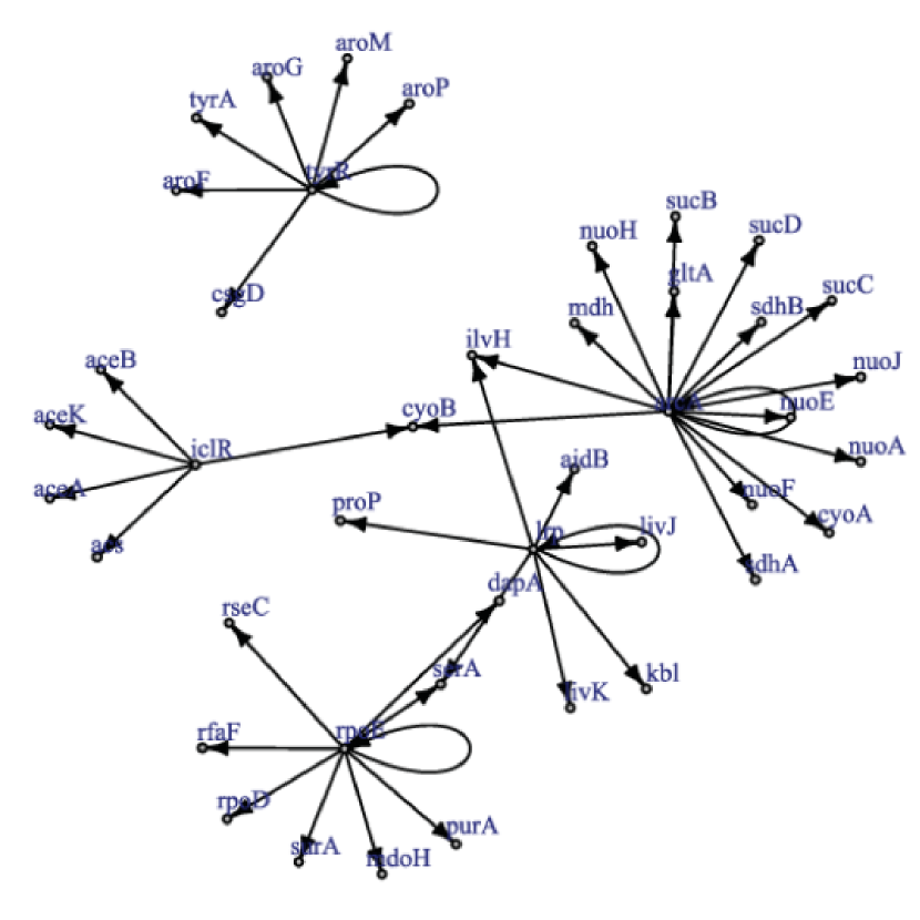
(a) E.Coli Network [10]

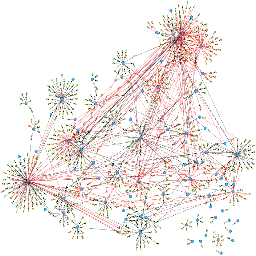
(b) Saccharomyces cerevisiae Network [33]

Figure 2(a) has only one edge violating the strong-causality assumption, and Figure 2(b) appears qualitatively to be nearly strongly causal. In particular, most of the edges are emanating from network hubs, and many of the other edges are colliders.

Figure 2(a) is reproduced under the Creative Commons Attribution Non-Commercial License (http://creativecommons.org/licenses/by-nc/2.5) and Figure 2(b) under the Creative Commons Attribution License (https://creativecommons.org/licenses/by/4.0/)

For later use, and to get a feel for the topological implications of strong causality, we explore a number of properties of such graphs before moving into the main result of this section. The following important property essentially strengthens Proposition 11 for the case of strongly causal graphs.

Proposition 5.

In a strongly causal graph if $j\in\mathcal{A}(i)$ then any $k\in\mathcal{A}(i)\cap\mathcal{A}(j)$ is not a confounder, that is, the unique path from $k$ to $i$ contains $j$.

Corollary 2.

If $\mathcal{G}$ is a strongly causal DAG then $i\overset{\text{PW}}{\rightarrow}j$ and $j\in\mathcal{A}(i)$ are alternatives, that is $i\overset{\text{PW}}{\rightarrow}j\Rightarrow j\notin\mathcal{A}(i)$.

Proof.

Suppose that $i\overset{\text{PW}}{\rightarrow}j$ and $j\in\mathcal{A}(i)$. Then since $\mathcal{G}$ is acyclic $i\not\in\mathcal{A}(j)$, and by Proposition 11 there is some $k\in\mathcal{A}(i)\cap\mathcal{A}(j)$ which is a confounder. However, by Proposition 12 $k$ cannot be a confounder, a contradiction. ∎

Corollary 3.

If $\mathcal{G}$ is a strongly causal DAG such that $i\overset{\text{PW}}{\rightarrow}j$ and $j\overset{\text{PW}}{\rightarrow}i$, then $i\not\in\mathcal{A}(j)$ and $j\not\in\mathcal{A}(i)$. In particular, a pairwise bidirectional edge indicates the absence of any edge in $\mathcal{G}$.

Proof.

This follows directly from applying Corollary 2 to $i\overset{\text{PW}}{\rightarrow}j$ and $j\overset{\text{PW}}{\rightarrow}i$. ∎

In light of Proposition 12, the following provides a partial converse to Proposition 11, and supports the intuition of “causal flow” through paths in $\mathcal{G}$.

Proposition 6.

If $\mathcal{G}$ is a strongly causal DAG then $j\in\mathcal{A}(i)\Rightarrow j\overset{\text{PW}}{\rightarrow}i$.

We immediately obtain the corollary, which we remind the reader is, surprisingly, not true in a general graph.

Corollary 4.

If $\mathcal{G}$ is a strongly causal DAG then $j\overset{\text{GC}}{\rightarrow}i\Rightarrow j\overset{\text{PW}}{\rightarrow}i$.

Example 4.

As a final remark of this subsection we note that a complete converse to Proposition 11 is not possible without additional conditions. Consider the “fork” system on $3$ nodes (i.e. $2\leftarrow 1\rightarrow 3$) defined by

$$x(t)=\left[\begin{array}[]{cccc}0&0&0\\ a&0&0\\ a&0&0\\ \end{array}\right]x(t-1)+v(t).$$

In this case, node $1$ is a confounder for nodes $2$ and $3$, but $x_{3}(t)=v_{3}(t)-v_{2}(t)+x_{2}(t)$ and $2\overset{\text{PW}}{\nrightarrow}3$ (even though $x_{2}(t)$ and $x_{3}(t)$ are contemporaneously correlated)

If we were to augment this system by simply adding an autoregressive component (i.e. some “memory”) to $x_{1}(t)$ e.g. $x_{1}(t)=v_{1}(t)+bx_{1}(t-1)$ then we would have $2\overset{\text{PW}}{\rightarrow}3$ since then $x_{3}(t)=v_{3}(t)+av_{1}(t-1)-bv_{2}(t-1)+bx_{2}(t-1)$. We develop this idea further in the next section.

2.6 Persistent Systems

In section 2.5 we obtained a converse to part $(a)$ of Proposition 11 via the notion of a strongly causal graph topology (see Proposition 13). In this section, we study conditions under which a converse to part $(b)$ will hold.

Definition 10 (Lag Function).

Given a causal filter $\mathsf{B}(z)=\sum_{\tau=0}^{\infty}b(\tau)z^{-\tau}$ define

$$\tau_{0}(\mathsf{B}) =\text{inf }\{\tau\in\mathbb{Z}_{+}\ |\ b(\tau)\neq 0\},$$ (9)

$$\tau_{\infty}(\mathsf{B}) =\text{sup }\{\tau\in\mathbb{Z}_{+}\ |\ b(\tau)\neq 0\}.$$ (10)

i.e. the “first” and “last” coefficients of the filter $\mathsf{B}(z)$, where $\tau_{\infty}(\mathsf{B})\overset{\Delta}{=}\infty$ if the filter has an infinite length, and $\tau_{0}(\mathsf{B})\overset{\Delta}{=}\infty$ if $\mathsf{B}(z)=0$.

Definition 11 (Persistent).

We will say that the process $x(t)$ with Granger causality graph $\mathcal{G}$ is persistent if for every $i\in[n]$ and every $k\in\mathcal{A}(i)$ we have $\tau_{0}(\mathsf{A}_{ik})<\infty$ and $\tau_{\infty}(\mathsf{A}_{ik})=\infty$.

Remark 3.

In the context of Granger causality, “most” systems should be persistent. In particular, $\mathsf{\mathsf{VAR}}(p)$ models are likely to be persistent since these naturally result in an equivalent $\mathsf{MA}(\infty)$ representation, see Example 5.

Moreover, persistence is not the weakest condition necessary for the results of this section, the condition that for each $i,j$ there is some $k\in\mathcal{A}(i)\cap\mathcal{A}(j)$ such that $\tau_{0}(\mathsf{A}_{jk})<\tau_{\infty}(\mathsf{A}_{ik})$ is enough. The intuition being that nodes $i$ and $j$ are not receiving temporally disjoint information from $k$.

The etymology for the persistence condition can be explained by supposing that the two nodes $i,j$ each have a loop (i.e. $\mathsf{B}_{ii}(z)\neq 0,\mathsf{B}_{jj}(z)\neq 0$) then this autoregressive component acts as “memory”, and so the influence from the confounder $k$ persists in $x_{i}(t)$, and $\tau_{\infty}(\mathsf{A}_{ik})=\infty$ for each confounder is expected.

Example 5.

Consider a process $x(t)$ generated by the $\mathsf{VAR}(1)$ model having $\mathsf{B}(z)=Bz^{-1}$. If $B$ is diagonalizable, and has at least $2$ distinct eigenvalues, then $x(t)$ is persistent.

See the supplementary material for an analysis of this example.

In order to eliminate the possibility of a particular sort of cancellation, an ad-hoc assumption is required. Strictly speaking, the persistence condition is not a necessary or sufficient condition for the following, but cases where the following fails to hold, and persistence does hold, are unavoidable pathologies.

Assumption 1.

Fix $i,j\in[n]$ and let $H_{i}(z)$ be the strictly-causal filter such that

$$H_{i}(z)x_{i}(t)=\hat{\mathbb{E}}[x_{i}(t)\ |\ \mathcal{H}_{t-1}^{(i)}],$$

and similarly for $H_{j}(z)$. Then define

$$T_{ij}(z)=\sum_{k\in\mathcal{A}(i)\cap\mathcal{A}(j)}\sigma_{k}^{2}\mathsf{A}_{ik}(z^{-1})(1-H_{i}(z^{-1}))(1-H_{j}(z))\mathsf{A}_{jk}(z),$$ (11)

where $\sigma_{k}^{2}=\mathbb{E}v_{k}(t)^{2}$.

We will say that Assumption 1 is satisfied if for every $i,j\in[n]$, $T_{ij}(z)$ is either constant over $z$ (i.e. each $z^{k}$ coefficient for $k\in\mathbb{Z}\setminus\{0\}$ is $0$), or is neither causal (i.e. containing only $z^{-k}$ terms, for $k\geq 0$) or anti-causal (i.e. containing only $z^{k}$ terms, for $k\geq 0$). Put succinctly, $T_{ij}(z)$ must be two-sided.

Remark 4.

Under the condition of persistence, the only way for Assumption 1 to fail is through cancellation in the terms defining $T_{ij}(z)$. For example, the condition is assured if $x(t)$ is persistent, and there is only a single confounder. Unfortunately, some pathological behaviour resulting from confounding nodes seems to be unavoidable without some assumptions about the parameters of the $\mathsf{MA}(\infty)$ system defining $x(t)$.

Proposition 7.

Fix $i,j\in[n]$ and suppose $\exists k\in\mathcal{A}(i)\cap\mathcal{A}(j)$ which confounds $i,j$. Then, if $T_{ij}(z)$ is not causal we have $j\overset{\text{PW}}{\rightarrow}i$, and if $T_{ij}(z)$ is not anti-causal we have $i\overset{\text{PW}}{\rightarrow}j$. Moreover, if Assumption 1 is satisfied, then $j\overset{\text{PW}}{\rightarrow}i\iff i\overset{\text{PW}}{\rightarrow}j$.

Remark 5.

The importance of this result is that when $i\overset{\text{PW}}{\rightarrow}j$ is a result of a confounder $k$, then $i\overset{\text{PW}}{\rightarrow}j\iff j\overset{\text{PW}}{\rightarrow}i$. This implies that in a strongly causal graph every bidirectional pairwise causality relation must be the result of a confounder. Therefore, in a strongly causal graph, pairwise causality analysis is immune to confounding (since we can safely remove all bidirectional edges).

2.7 Recovering $\mathcal{G}$ via Pairwise Tests

We arrive at the main conclusion of the theoretical analysis in this paper.

Theorem 2 (Pairwise Recovery).

If the Granger causality graph $\mathcal{G}$ for the process $x(t)$ is a strongly causal DAG and Assumption 1 holds, then $\mathcal{G}$ can be inferred from pairwise causality tests. The procedure can be carried out, assuming we have an oracle for pairwise causality, via Algorithm (2).

1

2 Algorithm:  Pairwise Graph Recovery

input : Pairwise Granger causality relations between a persistent process of dimension $n$ whose joint Granger causality relations are known to form a strongly causal DAG $\mathcal{G}$.

3

output : Edges $\mathcal{E}=\{(i,j)\in[n]\times[n]\ |\ i\overset{\text{GC}}{\rightarrow}j\}$ of the graph $\mathcal{G}$.

initialize : $S_{0}=[n]$ # unprocessed nodes

$E_{0}=\emptyset$ # edges of $\mathcal{G}$

$k=1$ # a counter used only for notation

4 $W\leftarrow\{(i,j)\ |\ i\overset{\text{PW}}{\rightarrow}j,j\overset{\text{PW}}{\nrightarrow}i\}$ # candidate edges

5 $P_{0}\leftarrow\{i\in S_{0}\ |\ \forall s\in S_{0}\ (s,i)\not\in W\}$ # parent-less nodes

6 while $S_{k-1}\neq\emptyset$ do

7       $S_{k}\leftarrow S_{k-1}\setminus P_{k-1}$ # remove nodes with depth $k-1$

8       $P_{k}\leftarrow\{i\in S_{k}\ |\ \forall s\in S_{k}\ (s,i)\not\in W\}$ # candidate children

9      

10      $D_{k0}\leftarrow\emptyset$

11       for $r=1,\ldots,k$ do

12             $Q\leftarrow E_{k-1}\cup\big{(}\bigcup_{\ell=0}^{r-1}D_{k\ell}\big{)}$ # currently known edges

13             $D_{kr}\leftarrow\{(i,j)\in P_{k-r}\times P_{k}\ |\ (i,j)\in W,\ \text{no }i\rightarrow j\text{ path in }Q\}$

14      $E_{k}\leftarrow E_{k-1}\cup\big{(}\bigcup_{r=1}^{k}D_{kr}\big{)}$ # update $E_{k}$ with new edges

15       $k\leftarrow k+1$

return $E_{k-1}$

Algorithm 1 Pairwise Granger Causality Algorithm

The theorem is proven in the supplementary material by establishing the correctness of Algorithm (2). The idea is to iteratively “peel away layers” of nodes by removing the nodes that have no parents remaining. The requirement of strong causality ensures that all actual edges of $\mathcal{G}$ manifest in some way as pairwise relations (by Proposition 13), and the no-cancellation condition of Assumption 1 allows confounding to be eliminated by removing bidirectional edges (by Proposition 14 and Corollary 3). Without Assumption 1, then each confounded pair would give rise to $4$ possible pairwise topologies consistent with $\mathcal{G}$, one for each type of pairwise edge (no edge, unidirectional, bidirectional).

Example 6.

The set $W$ collects ancestor relations in $\mathcal{G}$ (see Lemma 5). In reference to Figure 3, each of the solid black edges, as well as the dotted red edges will be included in $W$, but not the bidirectional green dash-dotted edges, which we are able to exclude as results of confounding. The groupings $P_{0},\ldots,P_{3}$ are also indicated in Figure 3.

The algorithm proceeds first with the parent-less nodes $1,2$ on the initial iteration where the edge $(1,3)$ is added to $E$. On the next iteration, the edges $(3,4),(2,4),(3,5)$ are added, and the false edges $(1,4),(1,5)$ are excluded due to the paths $1\rightarrow 3\rightarrow 4$ and $1\rightarrow 3\rightarrow 5$ already being present. Finally, edge $(4,6)$ is added, and the false $(1,6),(3,6),(2,6)$ edges are similarly excluded due to the ordering of the inner loop.

Figure 3: Example graph for Algorithm 2

Black arrows indicate true parent-child relations. Red dotted arrows indicate pairwise causality (due to non-parent relations), green dash-dotted arrows indicate bidirectional pairwise causality (due to the confounding node $1$). Blue groupings indicate each $P_{k}$ in Algorithm 2.

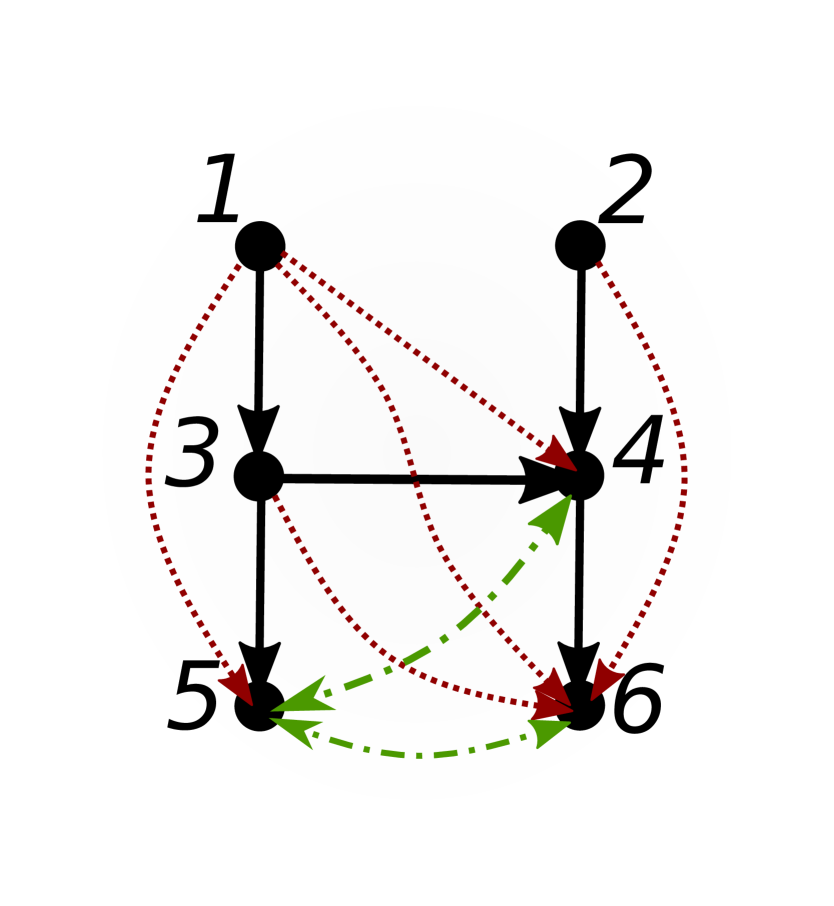
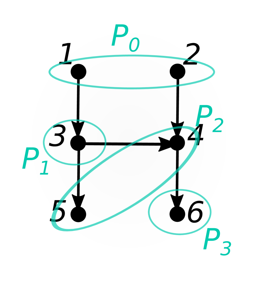
That we need to proceed backwards through $P_{k-r}$ as in the inner loop on $r$ can also be seen from this example, where if instead we simply added the set

$$D_{k}^{\prime}=\{(i,j)\in\Big{(}\bigcup_{r=1}^{k}P_{k-r}\Big{)}\times P_{k}\ |\ i\overset{\text{PW}}{\rightarrow}j\}$$

to $E_{k}$ then we would infer the false positive edge $1\rightarrow 4$. Moreover, the same example shows that simply using the set

$$D_{k}^{\prime\prime}=\{(i,j)\in P_{k-1}\times P_{k}\ |\ i\overset{\text{PW}}{\rightarrow}j\},$$

causes the edge $1\rightarrow 3$ to be missed.

3 Simulation

We implement an heuristic inspired by Algorithm 2 by replacing the population statistics with finite sample tests, the details of which can be found in the supplementary material Section C.5 (see Algorithm 3). The heuristic is essentially controlling the false discovery rate substantially below what it would be with a threshold based pairwise scheme. The methods are easily parallelizable, and can scale to graphs with thousands of nodes on a single machine. By contrast, scaling the LASSO to this large of a network (millions of variables) is nontrivial and extremely computationally demanding.

We run experiments using two separate graph topologies having $n=50$ nodes: a strongly causal graph (SCG) and a directed acyclic graph (DAG). Consult Section D for details on how data is generated from these models.

We compare our results against the adaptive LASSO [24], which outperformed both the LASSO and the grouped LASSO by a large margin. Motivated by scaling, we split the squared error term into separate terms, one for each group of incident edges on a node, and estimate the collection of $n$ incident filters $\big{\{}\mathsf{B}_{ij}(z)\big{\}}_{j=1}^{n}$ that minimizes $\xi_{i}^{\text{LASSO}}$ in the following:

$$\xi_{i}^{\text{LASSO}}(\lambda) =\underset{B}{\text{min}}\ \frac{1}{T}\sum_{t=p_{\text{max}}+1}^{T}\big{(}x_{i}(t)-\sum_{\tau=1}^{p_{\text{max}}}\sum_{j=1}^{n}B_{i,j}(\tau)x(t-\tau)\big{)}^{2}+\lambda\sum_{\tau=1}^{p_{\text{max}}}\sum_{j=1}^{n}|B_{ij}(\tau)|$$ (12)

$$\xi_{i}^{\text{LASSO}} =\underset{\lambda\geq 0}{\text{min}}\ \xi_{i}^{\text{LASSO}}(\lambda)+\mathsf{BIC}\big{(}B_{i}^{\text{LASSO}}(\lambda)\big{)}$$

where we are choosing $\lambda$, the regularization parameters, via the BIC. This is similar to the work of [34], except that we have replacing the LASSO with the Adaptive LASSO, which provides dramatically superior performance.

Figure 4: Representative Random Graph Topologies on $n=50$ Nodes

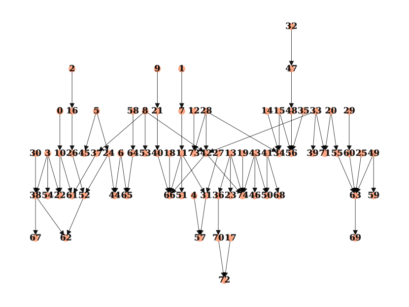
(a) SCG

(b) DAG $(q=\frac{2}{n})$

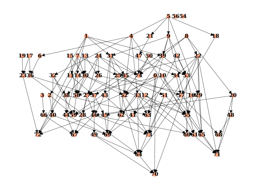
(c) DAG $(q=\frac{4}{n})$

Remark 6 (Graph Topologies).

We depict in Figure 4 the topologies of random graphs used in our empirical evaluation. For values of $q$ close to $\frac{2}{n}$, the resulting random graphs tend to have a topology which is, at least qualitatively, close to the SCG. As the value of $q$ increases, the random graphs deviate farther from the SCG topology, and we therefore expect the LASSO to outperform PWGC for larger values of $q$.

Remark 7 (MCC as a Support Recovery Measurement).

We apply Matthew’s Correlation Coefficient (MCC) [35] as a statistic for measuring support recovery performance (see also [36] tip # 8). This statistic synthesizes the confusion matrix into a single score appropriate for unbalanced labels and is calibrated to fall into the range $[-1,1]$ with $1$ being perfect performance, $0$ being the performance of random guessing, and $-1$ being perfectly opposed.

Remark 8 (Error Measurement).

We estimate the 1-step ahead prediction error by forming the variance matrix estimate

$$\widehat{\Sigma}_{v}\overset{\Delta}{=}\frac{1}{T_{\text{out}}}\sum_{t=1}^{T_{\text{out}}}(x(t)-\widehat{x}(t))(x(t)-\widehat{x}(t))^{\mathsf{T}}$$

on a long stream of out-of-sample data. We then report the quantity

$$\frac{\mathsf{ln\ }\mathsf{tr}\widehat{\Sigma}_{v}}{\mathsf{ln\ }\mathsf{tr}\Sigma_{v}}$$

where $\widehat{\Sigma}_{v}=\Sigma_{v}$ is the best possible performance.

3.1 Results

Figure 5: Simulation Results: PWGC vs AdaLASSO

	Algorithm	alasso	pwgc	alasso	pwgc	alasso	pwgc
	Metric	LRE		FDP		MCC
T	q
50	SCG	1.71	1.55	0.52	0.08	0.46	0.55
	0.04	1.97	1.77	0.57	0.10	0.41	0.53
	0.08	2.95	2.72	0.50	0.23	0.36	0.39
	0.32	9.02	8.17	0.53	0.56	0.14	0.10
250	SCG	1.30	1.18	0.29	0.06	0.70	0.81
	0.04	1.40	1.31	0.30	0.07	0.68	0.76
	0.08	2.49	2.21	0.32	0.16	0.55	0.57
	0.32	8.67	7.62	0.48	0.46	0.18	0.15
1250	SCG	1.20	1.11	0.41	0.07	0.68	0.88
	0.04	1.28	1.20	0.46	0.07	0.64	0.84
	0.08	2.12	2.05	0.36	0.14	0.60	0.64
	0.32	7.78	7.39	0.49	0.37	0.21	0.18

Results of Monte Carlo simulations comparing PWGC and AdaLASSO $(n=50,p=5,p_{\text{max}}=10)$ for small samples and when the SCG assumption doesn’t hold. The superior result is bolded when the difference is statistically significant, as measured by scipy.stats.ttest_rel. 100 iterations are run for each set of parameters.

LRE: Log-Relative-Error, i.e. the log sum of squared errors at each node relative to the strength of the driving noise $\frac{\mathsf{ln\ }\mathsf{tr}\widehat{\Sigma}_{v}}{\mathsf{ln\ }\mathsf{tr}\Sigma_{v}}$. FDP: False Discovery Proportion. MCC: Matthew’s Correlation Coefficient.

Values of $q$ (edge probability) range between $2/n,4/n,16/n$ where $2/n$ has the property that the random graphs have on average the same number of edges as the SCG.

Our simulation results are summarized in Table 5, with additional figures provided in the supplementary material Section D. It is clear that the superior performance of PWGC in comparison to AdaLASSO is as a result of limiting the false discovery rate. It is unsurprising that PWGC exhibits superior performance when the graph is an SCG, but even in the case of more general DAGs, the PWGC heuristic is still able to more reliably uncover the graph structure for small values of $q$. We would conjecture that for small $q$, random graphs are “likely” to be “close” to SCGs in some appropriate sense. As $q$ increases, there are simply not enough edges allowed by the SCG topology for it to be possible to accurately recover $\mathcal{G}$.

Interestingly, we can observe that the AdaLASSO appears to perform marginally better on strongly causal graphs than directed acyclic graphs with an equivalent number of edges ($q\approx 0.04$ is chosen for this purpose). This provides supporting evidence for one of the main assertions of this work: that the topological structure of $\mathcal{G}$ is an important distinguishing feature of time series networks in comparison to classical multivariate regression where it is only the sparsity rate which is considered.

4 Conclusion

In this paper we have argued that considering particular topological properties of Granger causality networks can provide substantial insights into the structure of causality graphs with potential for providing improvements to causality graph estimation when structural assumptions are met. In particular, the notion of a strongly-causal graph has been exploited to establish conditions under which pairwise causality testing alone is sufficient for recovering a complete Granger causality graph. Moreover, examples from the literature suggest that such topological assumptions may be reasonable in some applications. And secondly, even when the strong-causality assumption is not met, we have provided simulation evidence to suggest that our pairwise testing algorithm PWGC can still outperform the LASSO and adaLASSO, both of which are commonly employed in applications.

We emphasize that the causality graph topology is one of the key defining features of time series analysis in comparison to standard multivariate regression and therefore advocate for further study of how different topological assumptions may impact the recovery of causality graphs. For example, are there provable guarantees on the error rate of PWGC when applied to non strongly-causal graphs? Can constraint systems or cunning adaptive weighting schemes impose useful prior knowledge about graph topology for the LASSO algorithm? Finally, the work of [28] has established the superiority of Granger causality testing by state space models (as opposed to pure autoregressions) in many cases. Combining this work with our PWGC algorithm (by modifying the approach described in Section C.1 to instead utilize state-space Granger causality testing) therefore is likely to enable application to very large networks of time series data which are not well approximated by finite $\mathsf{VAR}(p)$ models. Moreover, our heuristics are in principle applicable in a model-free context. As long as a primitive for testing the pairwise causation between two components of a multivariate time series is available, our methods may be useful.

Appendix A Overview

We restate our main results and provide detailed proofs. Simple Corollaries have their proofs in the main text, and are occasionally referenced here. The main Theorem is proven in Section B.2, and all of the building blocks are established in Section B.1.

We detail the methods used for our simulations and finite sample implementation in Section C and provide additional simulation results in Section D.

References to equations, lemmas, etc., in this document are prefixed with their section, whereas prefix-free equation numbers refer to the main document. e.g. “Equation (1)” refers to the first equation in the main document, and “Equation (A.1)” refers to the first equation in this document.

Code will be made available at https://github.com/RJTK/granger_causality, as well as accompanying this supplementary material.

Appendix B Proofs

B.1 Preparatory Results

Theorem 3 (Granger Causality Equivalences 1).

The following are equivalent:

1. $x_{j}\overset{\text{GC}}{\nrightarrow}x_{i}$

2. $\forall\tau\in\mathbb{N}_{+}\ B_{ij}(\tau)=0$ i.e. $\mathsf{B}_{ij}(z)=0$

3. $H_{t}^{(i)}\perp\mathcal{H}_{t-1}^{(j)}\ |\ \mathcal{H}_{t-1}^{(-j)}$

4. $\hat{\mathbb{E}}[x_{i}(t)\ |\ \mathcal{H}_{t-1}^{(-j)}]=\hat{\mathbb{E}}[x_{i}(t)\ |\ \mathcal{H}_{t-1}]$

Proof.

$(a)\Rightarrow(b)$ follows as a result of the uniqueness of orthogonal projection (i.e. the best estimate is necessarily the coefficients of the model). $(b)\Rightarrow(c)$ follows since in computing $(y-\hat{\mathbb{E}}[y\ |\ \mathcal{H}_{t-1}^{(-j)}])$ for $y\in H_{t}^{(i)}$ it is sufficient to consider $y=x_{i}(t)$ by linearity, then since $H_{t-1}^{(i)}\subseteq\mathcal{H}_{t-1}^{(-j)}$ we have $(x_{i}(t)-\hat{\mathbb{E}}[x_{i}(t)\ |\ \mathcal{H}_{t-1}^{(-j)}])=v_{i}(t)$ since $\mathsf{B}_{ij}(z)=0$. The result follows since $v_{i}(t)\perp\mathcal{H}_{t-1}$. $(c)\iff(d)$ is a result of the equivalence in Definition 3. And, $(d)\implies(a)$ follows directly from the Definition. ∎

Lemma 1.

Let $S$ be the transposed adjacency matrix of the Granger causality graph $\mathcal{G}$. Then, $(S^{k})_{ij}$ is the number of paths of length $k$ from node $j$ to node $i$. Evidently, if $\forall k\in\mathbb{N},\ (S^{k})_{ij}=0$ then $j\not\in\mathcal{A}(i)$.

Proof.

This is a well known theorem, proof follows by induction. ∎

Proposition 8 (Ancestor Expansion).

The component $x_{i}(t)$ of $x(t)$ can be represented in terms of it’s parents in $\mathcal{G}$:

$$x_{i}(t)=v_{i}(t)+\mathsf{B}_{ii}(z)x_{i}(t)+\sum_{k\in pa(i)}\mathsf{B}_{ik}(z)x_{k}(t).$$ (B.1)

Moreover, $x_{i}$ can be expanded in terms of it’s ancestor’s $v(t)$ components only:

$$x_{i}(t)=\mathsf{A}_{ii}(z)v_{i}(t)+\sum_{\begin{subarray}{c}k\in\mathcal{A}(i)\\ k\neq i\end{subarray}}\mathsf{A}_{ik}(z)v_{k}(t),$$ (B.2)

where $\mathsf{A}(z)=\sum_{\tau=0}^{\infty}A(\tau)z^{-\tau}$ is the filter from the Wold decomposition representation of $x(t)$, Equation (2).

Proof.

Equation (B.1) is immediate from the $\mathsf{VAR}(\infty)$ representation of Equation (3) and Theorem 1, we are left to demonstrate (B.2).

From Equation (3), which we are assuming throughout the paper to be invertible, we can write

$$x(t)=(I-\mathsf{B}(z))^{-1}v(t),$$

where necessarily $(I-\mathsf{B}(z))^{-1}=\mathsf{A}(z)$ due to the uniqueness of the Wold decomposition. Since $\mathsf{B}(z)$ is stable we have

$$(I-\mathsf{B}(z))^{-1}=\sum_{k=0}^{\infty}\mathsf{B}(z)^{k}.$$ (B.3)

Invoking the Cayley-Hamilton theorem allows writing the infinite sum of (B.3) in terms of finite powers of $\mathsf{B}$.

Let $S$ be a matrix with elements in $\{0,1\}$ which represents the sparsity pattern of $\mathsf{B}(z)$, from Lemma 1 $S$ is the transpose of the adjacency matrix for $\mathcal{G}$ and hence $(S^{k})_{ij}$ is non-zero if and only if $j\in gp_{k}(i)$, and therefore $\mathsf{B}(z)^{k}_{ij}=0$ if $j\not\in gp_{k}(i)$. Finally, since $\mathcal{A}(i)=\bigcup_{k=1}^{n}gp_{k}(i)$ we see that $\mathsf{A}_{ij}(z)$ is zero if $j\not\in\mathcal{A}(i)$.

Therefore

$$x_{i}(t) =[(I-\mathsf{B}(z))^{-1}v(t)]_{i}$$

$$=\sum_{j=1}^{n}\mathsf{A}_{ij}(z)v_{j}(t)$$

$$=\mathsf{A}_{ii}(z)v_{i}(t)+\sum_{\begin{subarray}{c}j\in\mathcal{A}(i)\\ j\neq i\end{subarray}}\mathsf{A}_{ij}(z)v_{j}(t)$$

∎

Proposition 9.

Consider distinct nodes $i,j$ in a Granger causality graph $\mathcal{G}$. If

1. $j\not\in\mathcal{A}(i)$ and $i\not\in\mathcal{A}(j)$

2. $\mathcal{A}(i)\cap\mathcal{A}(j)=\emptyset$

then $\mathcal{H}_{t}^{(i)}\perp\mathcal{H}_{t}^{(j)}$, that is, $\forall s,\tau\in\mathbb{Z}_{+}\ \mathbb{E}[x_{i}(t-s)x_{j}(t-\tau)]=0$. Moreover, this means that $j\overset{\text{PW}}{\nrightarrow}i$ and $\hat{\mathbb{E}}[x_{j}(t)\ |\ \mathcal{H}_{t}^{(i)}]=0$.

Proof.

We show directly that $\forall s,\tau\in\mathbb{Z}_{+}\ \mathbb{E}[x_{i}(t-s)x_{j}(t-\tau)]=0$. To this end, fix $s,\tau\geq 0$, then by expanding with Equation (B.2) we have

$$\mathbb{E}x_{i}(t-s)x_{j}(t-\tau) =\mathbb{E}\big{(}\mathsf{A}_{ii}(z)v_{i}(t-s)\big{)}\big{(}\mathsf{A}_{jj}(z)v_{j}(t-\tau)\big{)}$$

$$+\sum_{\begin{subarray}{c}k\in\mathcal{A}(i)\\ k\neq i\end{subarray}}\mathbb{E}[\big{(}\mathsf{A}_{ik}(z)v_{k}(t-s)\big{)}\big{(}\mathsf{A}_{jj}(z)v_{j}(t-\tau)\big{)}]$$

$$+\sum_{\begin{subarray}{c}\ell\in\mathcal{A}(j)\\ \ell\neq j\end{subarray}}\mathbb{E}[\big{(}\mathsf{A}_{ii}(z)v_{i}(t-s)\big{)}\big{(}\mathsf{A}_{j\ell}(z)v_{\ell}(t-\tau)\big{)}]$$

$$+\sum_{\begin{subarray}{c}k\in\mathcal{A}(i)\\ k\neq i\end{subarray}}\sum_{\begin{subarray}{c}\ell\in\mathcal{A}(j)\\ \ell\neq j\end{subarray}}\mathbb{E}[\big{(}\mathsf{A}_{ik}(z)v_{k}(t-s)\big{)}\big{(}\mathsf{A}_{j\ell}(z)v_{\ell}(t-\tau)\big{)}].$$

Keeping in mind that $v(t)$ is an isotropic and uncorrelated sequence we see that each of these above four terms are 0: the first term since $i\neq j$, the second and third since $j\not\in\mathcal{A}(i)$ and $i\not\in\mathcal{A}(j)$ and finally the fourth since $\mathcal{A}(i)\cap\mathcal{A}(j)=\emptyset$. ∎

Lemma 2.

Consider distinct nodes $i,j$ in a Granger causality graph $\mathcal{G}$. If $j\not\in\mathcal{A}(i)$, then $\mathcal{H}_{t}^{(v_{j})}\perp\mathcal{H}_{t}^{(i)}$, and therefore for any causal filter $\Phi(z)$ we have

$$\hat{\mathbb{E}}[\Phi(z)v_{j}(t)\ |\ \mathcal{H}_{t-1}^{(i)}] =0$$

$$\langle x_{i}(t),\Phi(z)v_{j}(t)\rangle =0.$$

Proof.

Fix $\tau,s\geq 0$, then by expanding with Equation (B.2)

$$\mathbb{E}[x_{i}(t-\tau)v_{j}(t-s)] =\mathbb{E}[\big{(}\mathsf{A}_{ii}(z)v_{i}(t)+\sum_{k\in\mathcal{A}(i)}\mathsf{A}_{ik}(z)v_{k}(t)\big{)}v_{j}(t-s)]$$

$$=0.$$

This follows since $i\neq j$ and $j\not\in\mathcal{A}(i)$ and $v(t)$ is isotrophic and uncorrelated. ∎

Proposition 10.

Consider distinct nodes $i,j$ in a Granger causality graph $\mathcal{G}$. If

1. $j\not\in\mathcal{A}(i)$

2. $\mathcal{A}(i)\cap\mathcal{A}(j)=\emptyset$

then $j\overset{\text{PW}}{\nrightarrow}i$.

Proof.

By Theorem 1 it suffices to show that

$$\forall\psi\in\mathcal{H}_{t-1}^{(j)}\ \langle x_{i}(t)-\hat{\mathbb{E}}[x_{i}(t)\ |\ \mathcal{H}_{t-1}^{(i)}],\psi-\hat{\mathbb{E}}[\psi\ |\ \mathcal{H}_{t-1}^{(i)}]\rangle=0.$$

which by the orthogonality principle and by representing $\psi\in\mathcal{H}_{t-1}^{(j)}$ via the action of some strictly causal filter $\Phi(z)$ on $x_{j}(t)$ is equivalent to

$$\langle x_{i}(t),\Phi(z)x_{j}(t)-\hat{\mathbb{E}}[\Phi(z)x_{j}(t)\ |\ \mathcal{H}_{t-1}^{(i)}]\rangle=0.$$ (B.4)

If we expand $x_{j}(t)$ using Equation (B.2), the left hand side of (B.4) becomes

$$\langle x_{i}(t),\sum_{k\in\mathcal{A}(j)\cup\{j\}}\Big{(}\Phi(z)\mathsf{A}_{jk}(z)v_{k}(t)-\hat{\mathbb{E}}[\Phi(z)\mathsf{A}_{jk}(z)v_{k}(t)\ |\ \mathcal{H}_{t-1}^{(i)}]\Big{)}\rangle.$$

We see that this is $0$ by Lemma 2 since $j\not\in\mathcal{A}(i)$, and

$$\mathcal{A}(i)\cap\mathcal{A}(j)=\emptyset\implies\forall k\in\mathcal{A}(j):k\not\in\mathcal{A}(i).$$

∎

Remark 9.

In order to prove Proposition 11 we require some additional notation, as well as another representation theorem. The difficulty addressed by the following Definition 12 and Lemma 3 is that in the representation of $x_{j}(t)$ in terms of it’s parents (i.e. Equation (B.1))

$$x_{i}(t)=v_{i}(t)+\mathsf{B}_{ii}(z)x_{i}(t)+\sum_{k\in pa(i)}\mathsf{B}_{ik}(z)x_{k}(t),$$

the filter $\mathsf{B}_{ii}(z)$ need not be stable. That is, the inverse filter $(1-\mathsf{B}_{ii}(z))^{-1}$ need not exist. An example of this issue is furnished by

$$\mathsf{B}(z)=\left[\begin{array}[]{cc}\rho&-a\\ a&0\\ \end{array}\right]z^{-1},$$

for which, depending on the value of $a$, may still be stable even if $|\rho|>1$. This implies that it is not always possible to represent $x_{i}(t)$ in terms of $v_{i}(t)$ and $x_{k}(t),k\in pa(i)$ alone, i.e. as

$$x_{i}(t)=(1-\mathsf{B}_{ii}(z))^{-1}\big{(}v_{i}(t)+\sum_{k\in pa(i)}\mathsf{B}_{ik}(z)x_{k}(t)\big{)}.$$

The difficulty presented by the non-existence of such a representation may become apparent upon studying the proof of Proposition 11.

Definition 12 (Strongly Connected Components).

In a graph $\mathcal{G}$, the ordered (by the natural ordering on $\mathbb{N}$) subset $S\subseteq[n]$ is strongly connected if $\forall i,j\in S$, $i\in\mathcal{A}(j)$ and $j\in\mathcal{A}(i)$. We will denote by $S(j)$ (which may be the singleton $(j)$) the largest strongly connected component (SCC) containing $j$. We will denote $x_{S(j)}(t)$ to be the vector of processes

$$x_{S(j)}(t)=\big{(}x_{s}(t)\ |\ s\in S(j)\big{)},$$

whose indices are given the same (natural) ordering as $S(j)$. Similarly, the sub-filter of $\mathsf{B}(z)$ acting on $x_{S(j)}(t)$ will be denoted $\mathsf{B}_{S(j)}(z)$.

Lemma 3 (Expansion in SCCs).

Given some $j\in[n]$, the process $x_{S(j)}(t)$ can be represented by

$$x_{S(j)}(t)=v_{S(j)}(t)+\mathsf{B}_{S(j)}(z)x_{S(j)}(t)+\sum_{\begin{subarray}{c}s\in S(j)\\ k\in pa(s)\cap S(j)^{\mathsf{c}}\end{subarray}}B_{sk}(z)x_{k}(t)e_{s}^{S(j)},$$ (B.5)

where $e_{s}^{S(j)}$ denotes the length $|S(j)|$ canonical basis vector with a $1$ in the component corresponding to $x_{s}$ in the vector $x_{S(j)}$, and the summation is a double sum on $s$ and $k$.

Moreover, the filter $\mathsf{B}(z)$ is stable with $I-\mathsf{B}_{S(j)}(z)$ invertible:

$$(I-\mathsf{B}_{S(j)}(z))^{-1}=\sum_{k=0}^{\infty}\mathsf{B}_{S(j)}(z)^{k},$$ (B.6)

therefore

$$x_{S(j)}(t)=(I-\mathsf{B}_{S(j)}(z))^{-1}\big{(}v_{S(j)}(t)+\sum_{\begin{subarray}{c}s\in S(j)\\ k\in pa(s)\cap S(j)^{\mathsf{c}}\end{subarray}}B_{sk}(z)x_{k}(t)e_{s}^{S(j)}\big{)}.$$ (B.7)

Proof.

The representation of Equation (B.5) follows directly from the $\mathsf{VAR}$ representation of $x(t)$ (i.e. Equation (3))

$$x(t)=\mathsf{B}(z)x(t)+v(t),$$

which, when rearranged appropriately, can be written as

$$\left[\begin{array}[]{c}x_{S(j)}(t)\\ x_{S(j)^{c}}(t)\end{array}\right]=\left[\begin{array}[]{cc}\mathsf{B}_{S(j)}(z)&\mathsf{B}_{S(j),S(j)^{\mathsf{c}}}(z)\\ \mathsf{B}_{S(j)^{\mathsf{c}},S(j)}(z)&\mathsf{B}_{S(j)^{\mathsf{c}}}(z)\end{array}\right]\left[\begin{array}[]{c}x_{S(j)}(t)\\ x_{S(j)^{c}}(t)\end{array}\right]+\left[\begin{array}[]{c}v_{S(j)}(t)\\ v_{S(j)^{c}}(t)\end{array}\right].$$

Theorem 1 is invoked in order to restrict the summation to $k\in pa(s)$ (since other elements are $0$).

Now, we can partition $\mathcal{G}$ into it’s maximal SCCs $S_{1},\ldots,S_{N}$, (one of which is $S(j)$) and then consider the DAG formed on $N$ nodes with edges $I\rightarrow J$ included on the condition that $\exists j\in S_{J},i\in S_{I}\text{ s.t. }i\in\mathcal{A}(j)$. By topologically sorting this DAG, we obtain an ordering $\sigma$ of $[n]$ such that $\mathsf{B}_{\sigma}(z)$ is block upper triangluar, with one of it’s diagonal blocks consisting of the (possibly reordered) matrix $\mathsf{B}_{S(j)}(z)$. So we have

$$\forall\ |z^{-1}|\leq 1:\det\mathsf{B}(z)=\prod_{i=1}^{N}\det\mathsf{B}_{S_{i}}(z) \neq 0$$

$$\implies\forall\ |z^{-1}|\leq 1:\det\mathsf{B}_{S(j)}(z) \neq 0,$$

and therefore $\mathsf{B}_{S(j)}(z)$ is stable, invertible, and Equation (B.6) holds. ∎

Proposition 11.

If in a Granger causality graph $\mathcal{G}$ where $j\overset{\text{PW}}{\rightarrow}i$ then $j\in\mathcal{A}(i)$ or $\exists k\in\mathcal{A}(i)\cap\mathcal{A}(j)$ which is a confounder of $(i,j)$.

Proof.

We will prove by way of contradiction. To this end, suppose that $j$ is a node such that:

1. $j\not\in\mathcal{A}(i)$

2. every $k\in\mathcal{A}(i)\cap\mathcal{A}(j)$ every $k\rightarrow\cdots\rightarrow j$ path contains $i$.

Firstly, notice that every $u\in\big{(}pa(j)\setminus\{i\}\big{)}$ necessarily inherits these same two properties. This follows since if we also had $u\in\mathcal{A}(i)$ then $u\in\mathcal{A}(i)\cap\mathcal{A}(j)$ so by our assumption every $u\rightarrow\cdots\rightarrow j$ path must contain $i$, but $u\in pa(j)$ so $u\rightarrow j$ is a path that doesn’t contain $i$, and therefore $u\not\in\mathcal{A}(i)$; moreover, if we consider $w\in\mathcal{A}(i)\cap\mathcal{A}(u)$ then we also have $w\in\mathcal{A}(i)\cap\mathcal{A}(j)$ so the assumption implies that every $w\rightarrow\cdots\rightarrow j$ path must contain $i$. These properties therefore extend inductively to every $u\in\big{(}\mathcal{A}(j)\setminus\{i\}\big{)}$.

In order to deploy a recursive argument, define the following partition of $pa(u)$, for some node $u$:

$$C_{0}(u) =\{k\in pa(u)\ |\ i\not\in\mathcal{A}(k),\mathcal{A}(i)\cap\mathcal{A}(k)=\emptyset,k\neq i\}$$

$$C_{1}(u) =\{k\in pa(u)\ |\ i\in\mathcal{A}(k)\text{ or }k=i\}$$

$$C_{2}(u) =\{k\in pa(u)\ |\ i\not\in\mathcal{A}(k),\mathcal{A}(i)\cap\mathcal{A}(k)\neq\emptyset,k\neq i\}.$$

We notice that for any $u$ having the properties $(a),(b)$ above, we must have $C_{2}(u)=\emptyset$ since if $k\in C_{2}(u)$ then $\exists w\in\mathcal{A}(i)\cap\mathcal{A}(k)$ (and $w\in\mathcal{A}(i)\cap\mathcal{A}(u)$, since $k\in pa(u)$) such that $i\not\in\mathcal{A}(k)$ and therefore there must be a path $w\rightarrow\cdots\rightarrow k\rightarrow u$ which does not contain $i$, contradicting property $(b)$. Moreover, for any $u\in\big{(}\mathcal{A}(j)\setminus\{i\}\big{)}$ and $k\in C_{0}(u)$, Proposition 10 shows that $H_{t}^{(i)}\perp\mathcal{H}_{t-1}^{(j)}|\mathcal{H}_{t-1}^{(i)}$.

In order to establish $j\overset{\text{PW}}{\nrightarrow}i$, choose an arbitrary element of $\mathcal{H}_{t-1}^{(j)}$ and represent it via the action of a strictly causal filter $\Phi(z)$, i.e. $\Phi(z)x_{j}(t)\in\mathcal{H}_{t-1}^{(j)}$, by Theorem 1 it suffices to show that

$$\langle x_{i}(t),\Phi(z)x_{j}(t)-\hat{\mathbb{E}}[\Phi(z)x_{j}(t)\ |\ \mathcal{H}_{t-1}^{(i)}]\rangle=0.$$ (B.8)

Denote $e_{j}\overset{\Delta}{=}e_{j}^{S(j)}$, we can write $x_{j}(t)=e_{j}^{\mathsf{T}}x_{S(j)}(t)$, and therefore from Equation (B.7) there exist strictly causal filters $\Gamma_{s}(z)$ and $\Lambda_{sk}(z)$ (defined for ease of notation) such that

$$x_{j}(t)=\sum_{s\in S(j)}\Gamma_{s}(z)v_{s}(t)+\sum_{\begin{subarray}{c}s\in S(j)\\ k\in pa(s)\cap S(j)^{\mathsf{c}}\end{subarray}}\Lambda_{sk}(z)x_{k}(t).$$

When we substitute this expression into the left hand side of Equation (B.8), we may cancel each term involving $v_{s}$ by Lemma 2, and each $k\in C_{0}(s)$ by our earlier argument, leaving us with

$$\sum_{\begin{subarray}{c}s\in S(j)\\ k\in C_{1}(s)\cap S(j)^{\mathsf{c}}\end{subarray}}\langle x_{i}(t),\Phi(z)\Lambda_{sk}(z)x_{k}(t)-\hat{\mathbb{E}}[\Phi(z)\Lambda_{sk}(z)x_{k}(t)\ |\ \mathcal{H}_{t-1}^{(i)}]\rangle.$$

Since each $k\in C_{1}(s)$ with $k\neq i$ inherits properties $(a)$ and $(b)$ above, we can recursively expand each $x_{k}$ of the above summation until reaching $k=i$ (which is garaunteed to terminate due to the definition of $C_{1}(u)$) which leaves us with some strictly causal filter $F(z)$ such that the left hand side of Equation (B.8) is equal to

$$\langle x_{i}(t),\Phi(z)F(z)x_{i}(t)-\hat{\mathbb{E}}[\Phi(z)F(z)x_{i}(t)\ |\ \mathcal{H}_{t-1}^{(i)}]\rangle,$$

and this is $0$ since $\Phi(z)F(z)x_{i}(t)\in\mathcal{H}_{t-1}^{(i)}$. ∎

Proposition 12.

In a strongly causal graph if $j\in\mathcal{A}(i)$ then any $k\in\mathcal{A}(i)\cap\mathcal{A}(j)$ is not a confounder, that is, the unique path from $k$ to $i$ contains $j$.

Proof.

Suppose that there is a path from $k$ to $i$ which does not contain $j$. In this case, there are multiple paths from $k$ to $i$ (one of which does go through $j$, since $j\in\mathcal{A}(i)$) which contradicts the assumption of strong causality. ∎

Proposition 13.

If $\mathcal{G}$ is a strongly causal DAG then $j\in\mathcal{A}(i)\Rightarrow j\overset{\text{PW}}{\rightarrow}i$.

Proof.

We will show that for some $\psi\in\mathcal{H}_{t-1}^{(j)}$ we have

$$\langle\psi-\hat{\mathbb{E}}[\psi\ |\ \mathcal{H}_{t-1}^{(i)}],x_{i}(t)-\hat{\mathbb{E}}[x_{i}(t)\ |\ \mathcal{H}_{t-1}^{(i)}]\rangle\neq 0$$ (B.9)

and therefore that $H_{t}^{(i)}\not\perp\ \mathcal{H}_{t-1}^{(j)}\ |\ \mathcal{H}_{t-1}^{(i)}$, which by Theorem (1) is enough to establish that $j\overset{\text{PW}}{\rightarrow}i$.

Firstly, we will establish a representation of $x_{i}(t)$ that involves $x_{j}(t)$. Denote by $a_{r+1}\rightarrow a_{r}\rightarrow\cdots\rightarrow a_{1}\rightarrow a_{0}$ with $a_{r+1}\overset{\Delta}{=}j$ and $a_{0}\overset{\Delta}{=}i$ the unique $j\rightarrow\cdots\rightarrow i$ path in $\mathcal{G}$, we will expand the representation of Equation (B.1) backwards along this path:

$$x_{i}(t) =v_{i}(t)+\mathsf{B}_{ii}(z)x_{i}(t)+\sum_{k\in pa(i)}\mathsf{B}_{ik}(z)x_{k}(t)$$

$$=\underbrace{v_{a_{0}}(t)+\mathsf{B}_{a_{0}a_{0}}(z)x_{i}(t)+\sum_{\begin{subarray}{c}k\in pa(a_{0})\\ k\neq a_{1}\end{subarray}}\mathsf{B}_{a_{0}k}(z)x_{k}(t)}_{\overset{\Delta}{=}\widetilde{\alpha}(a_{0},a_{1})}+\mathsf{B}_{a_{0}a_{1}}(z)x_{a_{1}}(t)$$

$$=\widetilde{\alpha}(a_{0},a_{1})+\mathsf{B}_{a_{0}a_{1}}(z)\big{[}\widetilde{\alpha}(a_{1},a_{2})+\mathsf{B}_{a_{1}a_{2}}(z)x_{a_{2}}(t)\big{]}$$

$$\overset{(a)}{=}\sum_{\ell=0}^{r}\underbrace{\Big{(}\prod_{m=0}^{\ell-1}\mathsf{B}_{a_{m}a_{m+1}}(z)\Big{)}}_{\overset{\Delta}{=}F_{\ell}(z)}\widetilde{\alpha}(a_{\ell},a_{\ell+1})+\Big{(}\prod_{m=0}^{r}\mathsf{B}_{a_{m}a_{m+1}}(z)\Big{)}x_{a_{r+1}}(t)$$

$$=\sum_{\ell=0}^{r}F_{\ell}(z)\widetilde{\alpha}(a_{\ell},a_{\ell+1})+F_{r+1}(z)x_{j}(t)$$

where $(a)$ follows by a routine induction argument and where we define $\prod_{m=0}^{-1}\bullet\overset{\Delta}{=}1$ for notational convenience.

Using this representation to expand Equation (B.9), we obtain the following cumbersome expression:

$$\langle\psi-\hat{\mathbb{E}}[\psi\ |\ \mathcal{H}_{t-1}^{(i)}],F_{r+1}(z)x_{j}(t)-\hat{\mathbb{E}}[F_{r+1}(z)x_{j}(t)\ |\ \mathcal{H}_{t-1}^{(i)}]\rangle$$

$$-\langle\psi-\hat{\mathbb{E}}[\psi\ |\ \mathcal{H}_{t-1}^{(i)}],\hat{\mathbb{E}}[\sum_{\ell=0}^{r}F_{\ell}(z)\widetilde{\alpha}(a_{\ell},a_{\ell+1})\ |\ \mathcal{H}_{t-1}^{(i)}]\rangle$$

$$+\langle\psi-\hat{\mathbb{E}}[\psi\ |\ \mathcal{H}_{t-1}^{(i)}],\sum_{\ell=0}^{r}F_{\ell}(z)\widetilde{\alpha}(a_{\ell},a_{\ell+1})\rangle.$$

Note that by the orthogonality principle, $\psi-\hat{\mathbb{E}}[\psi\ |\ \mathcal{H}_{t-1}^{(i)}]\perp\mathcal{H}_{t-1}^{(i)}$, the middle term above is $0$. Choosing now the particular value $\psi=F_{r+1}(z)x_{j}(t)\in\mathcal{H}_{t-1}^{(j)}$ we arrive at

$$\langle\psi-\hat{\mathbb{E}}[\psi\ |\ \mathcal{H}_{t-1}^{(i)}],x_{i}(t)-\hat{\mathbb{E}}[x_{i}(t)\ |\ \mathcal{H}_{t-1}^{(i)}]\rangle$$

$$=\mathbb{E}|F_{r+1}(z)x_{j}(t)-\hat{\mathbb{E}}[F_{r+1}(z)x_{j}(t)\ |\ \mathcal{H}_{t-1}^{(i)}]|^{2}$$

$$+\langle F_{r+1}(z)x_{j}(t)-\hat{\mathbb{E}}[F_{r+1}(z)x_{j}(t)\ |\ \mathcal{H}_{t-1}^{(i)}],\sum_{\ell=0}^{r}F_{\ell}(z)\widetilde{\alpha}(a_{\ell},a_{\ell+1})\rangle.$$

Now since $F_{r+1}(z)\neq 0$ by Theorem 1, and $F_{r+1}(z)x_{j}(t)\not\in\mathcal{H}_{t-1}^{(i)}$, we have by the Cauchy-Schwarz inequality that this expression is equal to $0$ if and only if

$$\sum_{\ell=0}^{r}F_{\ell}(z)\widetilde{\alpha}(a_{\ell},a_{\ell+1})\overset{\text{a.s.}}{=}\hat{\mathbb{E}}[F_{r+1}(z)x_{j}(t)\ |\ \mathcal{H}_{t-1}^{(i)}]-F_{r+1}(z)x_{j}(t),$$

or by rearranging and applying the representation for $x_{i}(t)$ obtained earlier, if and only if

$$x_{i}(t)\overset{\text{a.s.}}{=}\hat{\mathbb{E}}[F_{r+1}(z)x_{j}(t)\ |\ \mathcal{H}_{t-1}^{(i)}].$$

But, this is impossible since $x_{i}(t)\not\in\mathcal{H}_{t-1}^{(i)}$. ∎

Example 7.

Consider a process $x(t)$ generated by the $\mathsf{VAR}(1)$ model having $\mathsf{B}(z)=Bz^{-1}$. If $B$ is diagonalizable, and has at least $2$ distinct eigenvalues, then $x(t)$ is persistent.

Pick any $i\in[n],j\in\mathcal{A}(i)\setminus\{i\}$. Then the stability of $B$ allows us to write

$$\mathsf{A}(z)=\sum_{k=0}^{\infty}B^{k}z^{-k},$$

whereby we see that $\exists k>0$ such that $[B^{k}]_{ij}\neq 0$ (since $j\in\mathcal{A}(i)$). Then consider

_ij $$=e_{i}^{\mathsf{T}}B^{rk}e_{j}$$

$$\overset{(a)}{=}\big{(}(P^{\mathsf{T}}e_{i})^{\mathsf{T}}J^{rk}P^{-1}e_{j}\big{)}$$

$$=\mathsf{tr}[(P^{\mathsf{T}}e_{i})^{\mathsf{T}}J^{rk}P^{-1}e_{j}]$$

$$\overset{(b)}{=}\mathsf{tr}[(J^{rk})(vu^{\mathsf{T}})],$$

where $(a)$ utilizes the Jordan Normal Form of $B$, and $(b)$ denotes $u=P^{\mathsf{T}}e_{i}$ and $v=P^{-1}e_{j}$. In order for $\tau_{\infty}(\mathsf{A}_{ij})<\infty$, there must be some $N>1$ such that $\forall r\geq N$, the above term is $0$. This may be the case for instance if $B$ is a nilpotent matrix.

Using the supposition that $B$ is diagonalizable (i.e. $J$ is a diagonal matrix) with at least $2$ distinct eigenvalues (in this case $B$ is not nilpotent), we can then rewrite the above as

$$f(r)\overset{\Delta}{=}\mathsf{tr}[(J^{rk})(vu^{\mathsf{T}})]=\sum_{\nu=1}^{n}\lambda_{\nu}^{rk}v_{\nu}u_{\nu}\overset{\Delta}{=}\sum_{\nu=1}^{n}\lambda_{\nu}^{rk}\beta_{\nu}$$

where $\lambda_{\nu}$ denotes the eigenvalues of $B$ and $\beta_{\nu}=u_{\nu}v_{\nu}$. Note that $f(0)=0$ since $i\neq j$ and $u$ is a row of $P$ and $v$ is a column of $P^{-1}$. Moreover, $f(1)\neq 0$ by hypothesis. But, in order for $f(r)=0\ \forall r\geq N$, it would need to be the case that

$$\mathsf{Dg}(\bm{\lambda})^{r}\bm{\lambda}=Vz$$

had a solution in $z$ for every $r\geq N$, where $V$ is an $n\times n-1$ full-rank matrix whose columns span the nullspace of $\beta$, and $\bm{\lambda}=(\lambda_{1},\ldots,\lambda_{n})$. That is, iterates of $\mathsf{Dg}(\bm{\lambda})$ applied to $\bm{\lambda}$ would need to remain inside $\beta$’s nullspace. This would imply that

$$VV^{\dagger}\bm{\lambda}^{r+1}=\bm{\lambda}^{r+1},$$

i.e. that $\bm{\lambda}^{r+1}$ is an eigenvector of $VV^{\dagger}$ for an infinite number of integers $r$ (the exponentiation is to be understood as a point wise operation). However, since there can only be a finite number of (unit length) eigenvectors, this cannot be the case unless every eigenvalue $(\lambda_{1},\ldots,\lambda_{n})$ were equal.

We see from this example that the collection of $\mathsf{VAR}(1)$ systems which are not persistent are pathological, in the sense that their system matrices have zero measure when viewed as a subset of $\mathbb{R}^{n^{2}}$.

Lemma 4.

Suppose $v(t)$ is a scalar process with unit variance and zero autocorrelation and let $\mathsf{A}(z),\mathsf{B}(z)$ be nonzero and strictly causal (i.e. $1\leq\tau_{0}(\mathsf{A})<\infty$, $1\leq\tau_{0}(\mathsf{B})<\infty$) linear filters. Then,

$$\langle F(z)\mathsf{A}(z)v(t),\mathsf{B}(z)v(t)\rangle=0\ \forall\text{ strictly causal filters }F(z)$$ (B.10)

if and only if $\tau_{0}(\mathsf{A})\geq\tau_{\infty}(\mathsf{B})$.

Proof.

We have

$$\langle\mathsf{A}(z)v(t),\mathsf{B}(z)v(t)\rangle =\sum_{\tau=1}^{\infty}\sum_{s=1}^{\infty}a(\tau)b(s)\mathbb{E}[v(t-s)v(t-\tau)]$$ (B.11)

$$=\sum_{\tau=\text{max}(\tau_{0}(\mathsf{A}),\tau_{0}(\mathsf{B}))}^{\text{min}(\tau_{\infty}(\mathsf{A}),\tau_{\infty}(\mathsf{B}))}a(\tau)b(\tau),$$ (B.12)

since $\mathbb{E}[v(t-s)v(t-\tau)]=\delta_{s-\tau}$. This expression is $0$ if and only if $\tau_{0}(\mathsf{A})\geq 1+\tau_{\infty}(\mathsf{B})$ or if $\tau_{0}(\mathsf{B})\geq 1+\tau_{\infty}(\mathsf{A})$ or if the coefficients are orthogonal along the common support.

Specializing this fact to $\langle F(z)\mathsf{A}(z)v(t),\mathsf{B}(z)v(t)\rangle$ we see that the coefficients cannot be orthogonal for every choice of $F$, and that $\text{sup}_{F}\tau_{\infty}(F\mathsf{A})=\infty$, leaving only the possibility that

$$\forall F\ \tau_{0}(F\mathsf{A})\geq 1+\tau_{\infty}(\mathsf{B}) \overset{(a)}{\iff}\tau_{0}(\mathsf{A})\geq 1+\tau_{\infty}(\mathsf{B})-\underset{F}{\text{min }}\tau_{0}(F)$$

$$\overset{(b)}{\iff}\tau_{0}(\mathsf{A})\geq\tau_{\infty}(\mathsf{B}),$$

where $(a)$ follows since $\tau_{0}(F\mathsf{A})=\tau_{0}(F)+\tau_{0}(\mathsf{A})$, and $(b)$ since $\text{min}_{F}\ \tau_{0}(F)=1$. ∎

Corollary 5.

For $k\in\mathcal{A}(i)\cap\mathcal{A}(j)$ we have

$$\hat{\mathbb{E}}[F(z)\mathsf{A}_{jk}(z)v_{k}(t)\ |\ \mathcal{H}_{t-1}^{(i)}] =0\ \forall\text{ strictly causal }F(z)$$

$$\iff\langle F(z)\mathsf{A}_{jk}(z)v_{k}(t),\mathsf{A}_{ik}(z)v_{k}(t)\rangle =0\ \forall\text{ strictly causal }F(z)$$

$$\iff\tau_{0}(\mathsf{A}_{jk})\geq\tau_{\infty}(\mathsf{A}_{ik})$$

Proof.

The final equivalence follows immediately from Lemma 4. For the first equivalence we have

$$\hat{\mathbb{E}}[F(z)\mathsf{A}_{jk}(z)v_{k}(t)\ |\ \mathcal{H}_{t-1}^{(i)}] =0\ \forall\text{ strictly causal }F(z)$$

$$\iff\langle F(z)A_{jk}(z)v_{k}(t),x_{i}(t-\tau)\rangle =0\ \forall\tau\geq 1,\text{ strictly causal }F(z),$$

which can be expanded by Equation (B.2) to obtain (after cancelling all ancestors of $i$ other than $k$)

$$\langle F(z)A_{jk}(z)v_{k}(t),\mathsf{A}_{ik}(z)v_{k}(t-\tau)\rangle=0\ \forall\tau\geq 1,\text{ strictly causal }F(z),$$

which by the Lemma is equivalent to $\tau_{0}(\mathsf{A}_{jk})\geq\tau_{\infty}(\mathsf{A}_{ik})$ as stated. ∎

Proposition 14.

Fix $i,j\in[n]$ and suppose $\exists k\in\mathcal{A}(i)\cap\mathcal{A}(j)$ which confounds $i,j$. Then, if $T_{ij}(z)$ is not causal we have $j\overset{\text{PW}}{\rightarrow}i$, and if $T_{ij}(z)$ is not anti-causal we have $i\overset{\text{PW}}{\rightarrow}j$. Moreover, if Assumption 1 is satisfied, then $j\overset{\text{PW}}{\rightarrow}i\iff i\overset{\text{PW}}{\rightarrow}j$.

Proof.

Recalling Theorem 1, consider some $\psi\in\mathcal{H}_{t-1}^{(j)}$ and represent it as $\psi(t)=F(z)x_{j}(t)$ for some strictly causal filter $F(z)$. Then

$$\langle\psi(t)-\hat{\mathbb{E}}[\psi(t)\ |\ \mathcal{H}_{t-1}^{(i)}],x_{i}(t)-\hat{\mathbb{E}}[x_{i}(t)\ |\ \mathcal{H}_{t-1}^{(i)}]\rangle$$

$$\overset{(a)}{=}\langle F(z)x_{j}(t),x_{i}(t)-\hat{\mathbb{E}}[x_{i}(t)\ |\ \mathcal{H}_{t-1}^{(i)}]\rangle$$

$$\overset{(b)}{=}\langle F(z)\big{(}\mathsf{A}_{jj}(z)v_{j}(t)+\sum_{k\in\mathcal{A}(j)}\mathsf{A}_{jk}(z)v_{k}(t)\big{)},(1-H_{i}(z))\big{(}\mathsf{A}_{ii}(z)v_{i}(t)+\sum_{\ell\in\mathcal{A}(i)}\mathsf{A}_{i\ell}(z)v_{\ell}(t)\big{)}\rangle$$

$$\overset{(c)}{=}\sum_{k\in\mathcal{A}(i)\cap\mathcal{A}(j)}\langle F(z)\mathsf{A}_{jk}(z)v_{k}(t),(1-H_{i}(z))\mathsf{A}_{ik}(z)v_{k}(t)\rangle,$$

where $(a)$ applies the orthogonality principle, $(b)$ expands with Equation (B.2) with $H_{i}(z)x_{i}(t)=\hat{\mathbb{E}}[x_{i}(t)\ |\ H_{t-1}^{(i)}]$, and $(c)$ follows by performing cancellations of $v_{k}(t)\perp v_{\ell}(t)$ and noting that by the contrapositive of Proposition 12 we cannot have $i\in\mathcal{A}(j)$ or $j\in\mathcal{A}(i)$.

Through symmetric calculation, we can obtain the expression relevant to the determination of $i\overset{\text{PW}}{\rightarrow}j$ for $\phi\in\mathcal{H}_{t-1}^{(i)}$ represented by the strictly causal filter $G(z):\phi(t)=G(z)x_{i}(t)$

$$\langle\phi(t)-\hat{\mathbb{E}}[\phi(t)\ |\ \mathcal{H}_{t-1}^{(j)}],x_{j}(t)-\hat{\mathbb{E}}[x_{j}(t)\ |\ \mathcal{H}_{t-1}^{(j)}]\rangle$$

$$=\sum_{k\in\mathcal{A}(i)\cap\mathcal{A}(j)}\langle G(z)\mathsf{A}_{ik}(z)v_{k}(t),(1-H_{j}(z))\mathsf{A}_{jk}(z)v_{k}(t)\rangle,$$

where $H_{j}(z)x_{j}(t)=\hat{\mathbb{E}}[x_{j}(t)\ |\ \mathcal{H}_{t-1}^{(j)}].$

We have therefore

$$(j\overset{\text{PW}}{\rightarrow}i):\exists F(z)\text{ s.t. }\sum_{k\in\mathcal{A}(i)\cap\mathcal{A}(j)}\langle F(z)\mathsf{A}_{jk}(z)v_{k}(t),(1-H_{i}(z))\mathsf{A}_{ik}(z)v_{k}(t)\rangle\neq 0,$$ (B.14)

$$(i\overset{\text{PW}}{\rightarrow}j):\exists G(z)\text{ s.t. }\sum_{k\in\mathcal{A}(i)\cap\mathcal{A}(j)}\langle G(z)\mathsf{A}_{ik}(z)v_{k}(t),(1-H_{j}(z))\mathsf{A}_{jk}(z)v_{k}(t)\rangle\neq 0.$$ (B.15)

The persistence condition, by Corollary 5, ensures that for each $k\in\mathcal{A}(i)\cap\mathcal{A}(j)$ there is some $F(z)$ and some $G(z)$ such that at least one of the above terms constituting the sum over $k$ is non-zero. It remains to eliminate the possibility of cancellation in the sum.

The adjoint of a linear filter $C(z)$ is simply $C(z^{-1})$, which recall is strictly anti-causal if $C(z)$ is strictly causal. Using this, we can write

$$\sum_{k\in\mathcal{A}(i)\cap\mathcal{A}(j)}\langle F(z)\mathsf{A}_{jk}(z)v_{k}(t),(1-H_{i}(z))\mathsf{A}_{ik}(z)v_{k}(t)\rangle$$

$$= \sum_{k\in\mathcal{A}(i)\cap\mathcal{A}(j)}\langle\mathsf{A}_{ik}(z^{-1})(1-H_{i}(z^{-1}))F(z)\mathsf{A}_{jk}(z)v_{k}(t),v_{k}(t)\rangle.$$

Moreover, it is sufficient to find some strictly causal $F(z)$ of the form $F(z)(1-H_{j}(z))$ (abusing notation) since $1-H_{j}(z)$ is causal. Similarly for $G(z)$, this leads to symmetric expressions for $j\overset{\text{PW}}{\rightarrow}i$ and $i\overset{\text{PW}}{\rightarrow}j$ respectively:

$$\sum_{k\in\mathcal{A}(i)\cap\mathcal{A}(j)}\langle\mathsf{A}_{ik}(z^{-1})(1-H_{i}(z^{-1}))F(z)(1-H_{j}(z))\mathsf{A}_{jk}(z)v_{k}(t),v_{k}(t)\rangle,$$ (B.16)

$$\sum_{k\in\mathcal{A}(i)\cap\mathcal{A}(j)}\langle\mathsf{A}_{ik}(z^{-1})(1-H_{i}(z^{-1}))G(z^{-1})(1-H_{j}(z))\mathsf{A}_{jk}(z)v_{k}(t),v_{k}(t)\rangle.$$ (B.17)

Recall the filter from Assumption 1

$$T_{ij}(z)=\sum_{k\in\mathcal{A}(i)\cap\mathcal{A}(j)}\sigma_{k}^{2}\mathsf{A}_{ik}(z^{-1})(1-H_{i}(z^{-1}))(1-H_{j}(z))\mathsf{A}_{jk}(z).$$ (B.18)

Since each $v_{k}(t)$ is uncorrelated through time, $\langle T_{ij}(z)v_{k}(t),v_{k}(t)\rangle=\sigma_{k}^{2}T_{ij}(0)$, and therefore we have $j\overset{\text{PW}}{\rightarrow}i$ if $T_{ij}(z)$ is not causal and $i\overset{\text{PW}}{\rightarrow}j$ if $T_{ij}(z)$ it not anti-causal. Moreover, we have $i\overset{\text{PW}}{\nrightarrow}j$ and $j\overset{\text{PW}}{\rightarrow}i$ if $T_{ij}(z)$ is a constant. Therefore, under Assumption 1 $j\overset{\text{PW}}{\rightarrow}i\iff i\overset{\text{PW}}{\rightarrow}j$.

This follows since if $T_{ij}(z)$ is not causal then $\exists k>0$ such that the $z^{k}$ coefficient of $T_{ij}(z)$ is non-zero, and we can choose strictly causal $F(z)=z^{-k}$ such that (B.16) is non-zero and therefore $j\overset{\text{PW}}{\rightarrow}i$.

Similarly, if $T_{ij}(z)$ is not anti-causal, then $\exists k>0$ such that the $z^{-k}$ coefficient of $T_{ij}(z)$ is non-zero, and we can choose strictly causal $G(z)$ so that $G(z^{-1})=z^{k}$, and then B.17 is non-zero and therefore $i\overset{\text{PW}}{\rightarrow}j$. ∎

B.2 The Main Theorem

Theorem 4 (Pairwise Recovery).

If the Granger causality graph $\mathcal{G}$ for the process $x(t)$ is a strongly causal DAG and Assumption 1 holds, then $\mathcal{G}$ can be inferred from pairwise causality tests. The procedure can be carried out, assuming we have an oracle for pairwise causality, via Algorithm (2).

1

input : Pairwise Granger causality relations

output : Edges $\mathcal{E}=\{(i,j)\in[n]\times[n]\ |\ i\overset{\text{GC}}{\rightarrow}j\}$ of the graph $\mathcal{G}$.

initialize : $S_{0}=[n]$ # unprocessed nodes

$E_{0}=\emptyset$ # edges of $\mathcal{G}$

$k=1$ # a counter used only for notation

2 $W\leftarrow\{(i,j)\ |\ i\overset{\text{PW}}{\rightarrow}j,j\overset{\text{PW}}{\nrightarrow}i\}$ # candidate edges

3 $P_{0}\leftarrow\{i\in S_{0}\ |\ \forall s\in S_{0}\ (s,i)\not\in W\}$ # parentless nodes

4 while $S_{k-1}\neq\emptyset$ do

5       $S_{k}\leftarrow S_{k-1}\setminus P_{k-1}$ # remove nodes with depth $k-1$

6       $P_{k}\leftarrow\{i\in S_{k}\ |\ \forall s\in S_{k}\ (s,i)\not\in W\}$ # candidate children

7      

8      $D_{k0}\leftarrow\emptyset$

9       for $r=1,\ldots,k$ do

10             $Q\leftarrow E_{k-1}\cup\big{(}\bigcup_{\ell=0}^{r-1}D_{k\ell}\big{)}$ # currently known edges

11             $D_{kr}\leftarrow\{(i,j)\in P_{k-r}\times P_{k}\ |\ (i,j)\in W,\ \text{no }i\rightarrow j\text{ path in }Q\}$

12      $E_{k}\leftarrow E_{k-1}\cup\big{(}\bigcup_{r=1}^{k}D_{kr}\big{)}$ # update $E_{k}$ with new edges

13       $k\leftarrow k+1$

return $E_{k-1}$

Algorithm 2 Pairwise Granger Causality Algorithm (PWGC)

Our proof proceeds in 5 steps stated formally as lemmas. Firstly, we characterize the sets $W$ and $P_{k}$. Then we establish a correctness result for the inner loop on $r$, a correctness result for the outer loop on $k$, and finally that the algorithm terminates in a finite number of steps.

Lemma 5 ($W$ Represents Ancestor Relations).

In Algorithm 2 we have $(i,j)\in W$ if and only if $i\in\mathcal{A}(j)$. In particular, $W\subseteq\mathcal{E}$.

Proof.

Let $j\in[n]$ and suppose that $i\in\mathcal{A}(j)$. Then $i\overset{\text{PW}}{\rightarrow}j$ by Proposition 13. Proposition 12 ensures that $(i,j)$ are not confounded and Corollary 2 that $j\not\in\mathcal{A}(i)$ so $j\overset{\text{PW}}{\nrightarrow}i$ by Proposition and therefore 11 $(i,j)\in W$.

Conversely, suppose $(i,j)\in W$. Then since $j\overset{\text{PW}}{\nrightarrow}i$, Proposition 14 ensures that $(j,i)$ are not confounded and so by Proposition 11 we must have $i\in\mathcal{A}(j)$. ∎

Definition 13 (Depth).

For our present purposes we will define the depth $d(j)$ of a node $j$ in $\mathcal{G}$ to be the length of the longest path from a node in $P_{0}$ to $j$, where $d(j)=0$ if $j\in P_{0}$. It is apparent that such a path will always exist. For example, in Figure 3 we have $d(3)=1$ and $d(4)=2$.

Lemma 6 (Depth Characterization of $P_{k}$ and $S_{k}$).

$i\in P_{k}\iff d(i)=k$ and $j\in S_{k}\iff d(j)\geq k$.

Proof.

We proceed by induction, noting that $P_{0}$ is non-empty since $\mathcal{G}$ is acyclic and therefore $\mathcal{G}$ contains nodes without parents. The base case $i\in P_{0}\iff d(i)=0$ is by definition, and $j\in S_{0}\iff d(j)\geq 0$ is trivial since $S_{0}=[n]$. So suppose that the lemma is true up to $k-1$.

($i\in P_{k}\implies d(i)=k$): Let $i\in P_{k}$. Suppose that $d(i)\geq k+1$, then $\exists j\in pa(i)$ such that $j\not\in\cup_{r\geq 1}P_{k-r}$ (otherwise $d(i)\leq k$), this implies that $j\in S_{k}$ with $(j,i)\in W$ (by Lemma 5) which is not possible due to the construction of $P_{k}$ and therefore $d(i)\leq k$. Moreover, $P_{k}\subseteq S_{k}\subseteq S_{k-1}$ implies that $d(i)\geq k-1$ by the induction hypothesis, but if $d(i)=k-1$ then $i\in P_{k-1}$ again by induction which is impossible since $i\in P_{k}$ and therefore $d(i)=k$.

($s\in S_{k}\implies d(s)\geq k$): Let $s\in S_{k}\subseteq S_{k-1}$. We have by induction that $d(s)\geq k-1$, but again by induction (this time on $P_{k-1}$) we have $d(s)\neq k-1$ since $S_{k}=S_{k-1}\setminus P_{k-1}$ and therefore $d(s)\geq k$.

($d(i)=k\implies i\in P_{k}$): Suppose $i\in[n]$ is such that $d(i)=k$. Then $i\in S_{k-1}$ by the hypothesis, but also $i\not\in P_{k-1}$ so then $i\in S_{k}=S_{k-1}\setminus P_{k-1}$. Now, recalling the definition of $P_{k}$

$$P_{k}=\{i\in S_{k}\ |\ \forall s\in S_{k}\ (s,i)\not\in W\},$$

if $s\in S_{k}$ is such that $(s,i)\in W$ then $s\overset{\text{PW}}{\rightarrow}i$ and $i\overset{\text{PW}}{\nrightarrow}s$ so that by Proposition 14 there cannot be a confounder of $(s,i)$ (otherwise $i\overset{\text{PW}}{\rightarrow}s$) so then by Proposition 11 we have $s\in\mathcal{A}(i)$. We have shown that $s\in S_{k}\implies d(s)\geq k$ and so we must have $d(i)>k$, a contradiction, therefore there is no such $s\in S_{k}$ so $i\in P_{k}$.

($d(j)\geq k\implies j\in S_{k}$): Let $j\in[n]$ such that $d(j)\geq k$, then by induction we have $j\in S_{k-1}$. This implies by the construction of $S_{k}$ that $j\not\in S_{k}$ only if $j\in P_{k-1}$, but we have shown that this only occurs when $d(j)=k-1$, but $d(j)>k-1$ so $j\in S_{k}$. ∎

Lemma 7 (Inner Loop).

Fix an integer $k\geq 1$ and suppose that $(i,j)\in E_{k-1}$ if and only if $(i,j)\in\mathcal{E}$ and $d(j)\leq k-1$. Then, we have $(i,j)\in D_{kr}$ if and only if $(i,j)\in\mathcal{E}$, $d(j)=k$, and $d(i)=k-r$.

Proof.

We prove by induction on $r$, keeping in mind the results of Lemmas 5 and 6. For the base case, let $r=1$ and suppose that $(i,j)\in\mathcal{E}$ with $d(j)=k$ and $d(i)=k-1$. Then, by Corollary 4 $(i,j)\in W$ and by our assumptions on $E_{k-1}$ there is no $i\rightarrow\cdots\rightarrow j$ path in $E_{k-1}$ and therefore $(i,j)\in D_{k1}$. Conversely, suppose that $(i,j)\in D_{k1}$. Then, $d(i)=k-1$ and $d(j)=k$ which, since $(i,j)\in W\implies i\in\mathcal{A}(j)$ implies that $i\in pa(j)$ and $(i,j)\in\mathcal{E}$.

Now, fix $r>1$ and suppose that the result holds up to $r-1$. Let $(i,j)\in\mathcal{E}$ with $d(j)=k$ and $d(i)=k-r$. Then, $(i,j)\in W$ and by induction and strong causality there cannot already be an $i\rightarrow\cdots\rightarrow j$ path in $E_{k-1}\cup\big{(}\bigcup_{\ell=0}^{r-1}D_{kr}\big{)}$, therefore $(i,j)\in D_{kr}$. Conversely, suppose $(i,j)\in D_{kr}$. Then we have $d(i)=k-r$, $d(j)=k$, and $i\in\mathcal{A}(j)$. Suppose by way of contradiction that $i\not\in pa(j)$, then there must be some $u\in pa(j)$ such that $i\in\mathcal{A}(u)$. But, this implies that $d(i)<d(u)$ and by induction that $(u,j)\in\bigcup_{\ell=1}^{r-1}D_{k\ell}$. Moreover, since $d(u)<k$ (otherwise $d(j)>k$) each edge in the $i\rightarrow\cdots\rightarrow u$ path must already be in $E_{k-1}$, and so there must be an $i\rightarrow\cdots\rightarrow j$ path in $E_{k-1}\cup\big{(}\bigcup_{\ell=0}^{r-1}D_{kr}\big{)}$, which is a contradiction since we assumed $(i,j)\in D_{kr}$. Therefore $i\in pa(j)$ and $(i,j)\in\mathcal{E}$. ∎

Lemma 8 (Outer Loop).

We have $(i,j)\in E_{k}$ if and only if $(i,j)\in\mathcal{E}$ and $d(j)\leq k$. That is, at iteration $k,E_{k}$ and $\mathcal{E}$ agree on the set of edges whose terminating node is at most $k$ steps away from $P_{0}$.

Proof.

We will proceed by induction. The base case $E_{0}=\emptyset$ is trivial, so fix some $k\geq 1$, and suppose that the lemma holds for all nodes of depth less than $k$.

Suppose that $(i,j)\in E_{k}=E_{k-1}\cup\big{(}\bigcup_{r=1}^{k}D_{rk}\big{)}$. Then clearly there is some $1\leq r\leq k$ such that $(i,j)\in D_{kr}$ so that by Lemma 7 we have $(i,j)\in\mathcal{E}$ and $d(j)=k$.

Conversely, suppose that $(i,j)\in\mathcal{E}$ and $d(j)\leq k$. If $d(j)<k$ then by induction $(i,j)\in E_{k-1}\subseteq E_{k}$ so suppose further than $d(j)=k$. Since $i\in pa(j)$ we must have $d(i)<k$ (else $d(j)>k$) and again by Lemma 7 $(i,j)\in\bigcup_{r=1}^{k}D_{kr}$ which implies that $(i,j)\in E_{k}$. ∎

Lemma 9 (Finite Termination).

Algorithm 2 terminates and returns the set $E_{k^{\star}-1}=\mathcal{E}$ for some $k^{\star}\leq n$.

Proof.

If $n=1$, the algorithm is clearly correct, returning on the first iteration with $E_{1}=\emptyset$. When $n>1$ Lemma 8 ensures that $E_{k}$ coincides with $\{(i,j)\in\mathcal{E}\ |\ d(j)\leq k\}$ and since $d(j)\leq n-1$ for any $j\in[n]$ there is some $k^{\star}\leq n$ such that $E_{k^{\star}-1}=\mathcal{E}$. We must have $S_{k^{\star}}=\emptyset$ since $j\in S_{k^{\star}}\iff d(j)\geq k^{\star}$ (if $d(j)>k-1$ then $E_{k^{\star}-1}\neq\mathcal{E}$) and therefore the algorithm terminates. ∎

Appendix C Finite Sample Implementation

In this section we provide a review of our methods for implementing Algorithm 1 given a finite sample of $T$ data points. We apply the simplest reasonable methods in order to maintain a focus on our main contributions (i.e. Algorithm 2), more sophisticated schemes can only serve to improve the results. Textbook reviews of the following concepts are provided e.g. by [37], [38], and elsewhere.

In subsection C.1 we define pairwise Granger causality hypothesis tests, in subsection C.2 a model order selection criteria, in subsection C.3 an efficient estimation algorithm, in subsection C.4 the method for choosing an hypothesis testing threshold, and finally in subsection C.5 the unified finite sample algorithm.

C.1 Pairwise Hypothesis Testing

In performing pairwise checks for Granger causality $x_{j}\overset{\text{PW}}{\rightarrow}x_{i}$ we follow the simple scheme of estimating the following two linear models:

$$H_{0}: \ \widehat{x}_{i}^{(p)}(t)=\sum_{\tau=1}^{p}b_{ii}(\tau)x_{i}(t-\tau),$$ (C.1)

$$H_{1}: \ \widehat{x}_{i|j}^{(p)}(t)=\sum_{\tau=1}^{p}b_{ii}(\tau)x_{i}(t-\tau)+\sum_{\tau=1}^{p}b_{ij}(\tau)x_{j}(t-\tau).$$ (C.2)

We formulate the statistic

$$F_{ij}(p)=\frac{T}{p}\Big{(}\frac{\xi_{i}(p)}{\xi_{ij}(p)}-1\Big{)},$$ (C.3)

where $\xi_{i}(p)$ is the sample mean square of the residuals $x_{i}(t)-\widehat{x}^{(p)}_{i}(t)$,

$$\xi_{i}(p)=\frac{1}{T-p}\sum_{t=p+1}^{T}(x_{i}(t)-\widehat{x}_{i}^{(p)}(t))^{2},$$

and similarly for $\xi_{ij}(p)$. We test $F_{ij}(p)$ against a $\chi^{2}(p)$ distribution.

If the estimation procedure is consistent, we will have the following convergence (in $\mathbb{P}$ or a.s.):

$$F_{ij}(p)\rightarrow\left\{\begin{array}[]{ll}0;\ x_{j}\overset{\text{PW}}{\nrightarrow}x_{i}\\ \infty;\ x_{j}\overset{\text{PW}}{\rightarrow}x_{i}\end{array}\right.\text{ as }T\rightarrow\infty.$$ (C.4)

In our finite sample implementation (see Algorithm 3) we add edges to $\widehat{\mathcal{G}}$ in order of the decreasing magnitude of $F_{ij}$ instead of proceeding backwards through $P_{k-r}$ in Algorithm 2. This makes greater use of the information provided by the test statistic $F_{ij}$, moreover, if $x_{i}\overset{\text{GC}}{\rightarrow}x_{j}$ and $x_{j}\overset{\text{GC}}{\rightarrow}x_{k}$, it is expected that $F_{kj}>F_{ki}$, thereby providing the same effect as proceeding backwards through $P_{k-r}$.

C.2 Model Order Selection

There are a variety of methods to choose the filter order $p$ (see e.g. [39]), but we will focus in particular on the Bayesian Information Criteria (BIC). The BIC is substantially more conservative than the popular alternative Akaiake Information Criteria (the BIC is also asymptotically consistent), and since we are searching for sparse graphs, we therefore prefer the BIC, where we seek to minimize over $p$:

$$BIC_{\text{univariate}}(p) =\mathsf{ln\ }\ \xi_{i}(p)+p\frac{\mathsf{ln\ }T}{T},$$ (C.5)

$$BIC_{\text{bivariate}}(p) =\mathsf{ln\ }\det\widehat{\Sigma}_{ij}(p)+4p\frac{\mathsf{ln\ }T}{T},$$

where $\widehat{\Sigma}_{ij}(p)$ is the $2\times 2$ residual covariance matrix for the $\mathsf{VAR}(p)$ model of $(x_{i}(t),x_{j}(t))$. The bivariate errors $\xi_{ij}(p)$ and $\xi_{ji}(p)$ are the diagonal entries of $\widehat{\Sigma}_{ij}(p)$.

We carry this out by a simple direct search on each model order between $0$ and some prescribed $p_{\text{max}}$, resulting in a collection $p_{ij}$ of model order estimates. In practice, it is sufficient to pick $p_{\text{max}}$ ad-hoc or via some simple heuristic e.g. plotting the sequence $BIC(p)$ over $p$, though it is not technically possible to guarantee that the optimal $p$ is less than the chosen $p_{\text{max}}$ (since there can in general be arbitrarily long lags from one variable to another).

C.3 Efficient Model Estimation

In practice, the vast majority of computational effort involved in implementing our estimation algorithm is spent calculating the error estimates $\xi_{i}(p_{i})$ and $\xi_{ij}(p_{ij})$. This requires fitting a total of $n^{2}p_{\text{max}}$ autoregressive models, where the most naive algorithm (e.g. solving a least squares problem for each model) for this task will consume $O(n^{2}p_{\text{max}}^{4}T)$ time, it is possible to carry out this task in a much more modest $O(n^{2}p_{\text{max}}^{2})+O(n^{2}p_{\text{max}}T)$ time via the autocorrelation method [40] which substitutes the following autocovariance estimates in the Yule-Walker equations:

$$\widehat{R}_{x}(\tau)=\frac{1}{T}\sum_{t=\tau+1}^{T}x(t)x(t-\tau)^{\mathsf{T}};\ \tau=0,\ldots,p_{\text{max}},$$ (C.6)

It is imperative that the first index in the summation is $\tau+1$, as opposed perhaps to $p_{\text{max}}$ and that the normalization is $1/T$, as opposed perhaps to $1/(T-p_{\text{max}})$, in order to guarantee that $\widehat{R}_{x}(\tau)$ forms a valid (i.e. positive definite) covariance sequence. This results in some bias, however the dramatic computational speedup is worth it for our purposes.

These covariance estimates constitute the $O(n^{2}p_{\text{max}}T)$ operation. Given these particular estimates, the variances $\xi_{i}(p)$ for $p=1,\ldots,p_{\text{max}}$ can be evaluated in $O(p_{\text{max}}^{2})$ time each by applying the Levinson-Durbin recursion to $\widehat{R}_{ii}(\tau)$, which effectively estimates a sequence of $AR$ models, producing $\xi_{i}(p)$ as a side-effect (see [40] and [41]).

Similarly, the variance estimates $\widehat{\Sigma}_{ij}(p)$ (which include $\xi_{ij}$ and $\xi_{ji}$) can be obtained by estimating $\frac{(n+1)n}{2}$ bivariate AR models, again in $O(p_{\text{max}}^{2})$ time via Whittle’s generalized Levinson-Durbin recursion [42].

C.4 Edge Probabilities and Error Rate Controls

Denote $F_{ij}$ the Granger causality statistic of Equation (C.3) with model orders chosen by the methods of Section C.2. We assume that this statistic is asymptotically $\chi^{2}(p_{ij})$ distributed (e.g. the disturbances are Gaussian), and denote by $G$ the cumulative distribution function thereof. We will define the matrix

$$P_{ij}=G(F_{ij}),$$ (C.7)

to be the matrix of pairwise edge inclusion P-values. This is motivated by the hypothesis test where the hypothesis $H_{0}$ will be rejected (and thence we will conclude that $x_{j}\overset{\text{PW}}{\rightarrow}x_{i}$) if $P_{ij}>1-\delta$.

The value $\delta$ can be chosen by a variety of methods, in our case we apply the Benjamini Hochberg criteria [43] [37] to control the false discovery rate of pairwise edges to a level $\alpha$ (where we generally take $\alpha=0.05$).

C.5 Finite Sample Recovery Algorithm

After the graph topology $\widehat{\mathcal{G}}$ has been estimated via Algorithm 3, we refit the entire model with the specified sparsity pattern directly via ordinary least squares.

We note that producing graph estimates which are not strongly causal can potentially be achieved by performing sequential estimates $\widehat{x}_{1}(t),\widehat{x}_{2}(t),\ldots$ estimating a strongly causal graph with the residuals of the previous model as input, and then refitting on the combined sparsity pattern. We intend to consider this heuristic in future work.

1

2

input : Estimates of pairwise Granger causality statistics $F_{ij}$ (eqn. C.3). Matrix of edge probabilities $P_{ij}$ (eqn. C.7). Hypothesis testing threshold $\delta$ chosen via the Benjamini-Hochberg criterion (Section C.4)

output : A strongly causal graph $\widehat{\mathcal{G}}$

initialize : $S=[n]$ # unprocessed nodes

$E=\emptyset$ # edges of $\widehat{\mathcal{G}}$

$k=1$ # a counter used only for notation

3

4$W_{\delta}\leftarrow\{(i,j)\ |\ P_{ji}>1-\delta,F_{ji}>F_{ij}\}$ # candidate edges

5 $\mathcal{I}_{0}\leftarrow\big{(}\sum_{j\in S:(j,i)\in W_{\delta}}P_{ij},\mathsf{\ for\ }i\in S\big{)}$ # total node incident probability

6 $P_{0}\leftarrow\{i\in S\ |\ \mathcal{I}_{0}(i)<\lceil\text{min}(\mathcal{I}_{0})\rceil\}$ # Nodes with fewest incident edges

7 if $P_{0}=\emptyset$ then

8       $P_{0}\leftarrow\{i\in S\ |\ \mathcal{I}_{0}(i)\leq\lceil\text{min}(\mathcal{I}_{0})\rceil\}$ # Ensure non-empty

9

10while $S\neq\emptyset$ do

11       $S\leftarrow S\setminus P_{k-1}$ # remove processed nodes

12       $\mathcal{I}_{k}\leftarrow\big{(}\sum_{j\in S:(j,i)\in W_{\delta}}P_{ij},\mathsf{\ for\ }i\in S\big{)}$

13       $P_{k}\leftarrow\{i\in S\ |\ \mathcal{I}_{k}(i)<\lceil\text{min}(\mathcal{I}_{k})\rceil\}$

14       if $P_{k}=\emptyset$ then

15             $P_{k}\leftarrow\{i\in S\ |\ \mathcal{I}_{k}(i)\leq\lceil\text{min}(\mathcal{I}_{k})\rceil\}$

16      

17       # add strongest edges, maintaining strong causality

18       $U_{k}\leftarrow\bigcup_{r=1}^{k}P_{k-r}$ # Include all forward edges

19       for $(i,j)\in\mathsf{sort}\Big{(}\{(i,j)\in U_{k}\times P_{k}\ |\ (i,j)\in W_{\delta}\}\mathsf{\ by\ descending\ }F_{ji}\Big{)}$ do

20             if $\mathsf{is\_strongly\_causal}(E\cup\{(i,j)\})$ then

21                   # $\mathsf{is\_strongly\_causal}$ can be implemented by keeping

22                   # track of ancestor / descendant relationships

23                   $E\leftarrow E\cup\{(i,j)\}$

24            

25      $k\leftarrow k+1$

26      

return $([n],E)$

Algorithm 3 Finite Sample Pairwise Graph Recovery (PWGC)

Appendix D Simulation

We have implemented our empirical experiments in Python [44], in particular we leverage the LASSO implementation from sklearn [45] and the random graph generators from networkx [46]. We run experiments using two separate graph topologies having $n=50$ nodes. These are generated respectively by drawing a random tree and a random Erdos Renyi graph then creating a directed graph by directing edges from lower numbered nodes to higher numbered nodes.

We populate each of the edges (including self loops) with random linear filters constructed by placing $5$ transfer function poles (i.e. $p=5$) uniformly at random in a disc of radius $3/4$ (which guarantees stability for acyclic graphs). The resulting system is driven by i.i.d. Gaussian random noise, each component having random variance $\sigma_{i}^{2}=1/2+r_{i}$ where $r_{i}\sim\text{exp}(1/2)$. To ensure we are generating data from a stationary system, we first discard samples during a long burnin period.

For both PWGC and adaLASSO We set the maximum lag length $p_{\text{max}}=10$.

Results are collected in Figures 6, 7, 8, 9.

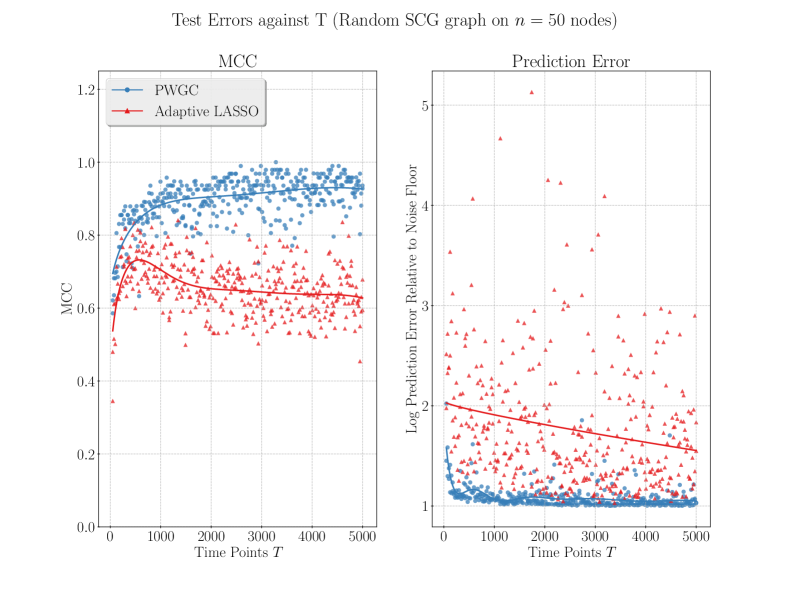
Figure 6: PWGC Compared Against AdaLASSO [24] (SCG)

Comparison of PWGC and LASSO for $\mathsf{VAR}(p)$ model estimation. We make comparisons against both the MCC and the relative log mean-squared prediction error $\frac{\mathsf{ln\ }\mathsf{tr}\widehat{\Sigma}_{v}}{\mathsf{ln\ }\mathsf{tr}\Sigma_{v}}$. Results in Figure 6 are for systems guaranteed to satisfy the assumptions required for Theorem 4.

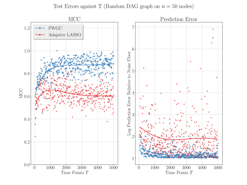
Figure 7: PWGC vs adaLASSO (DAG, $q=\frac{2}{n}$)

Figure 7 provides results for systems which do not guarantee the assumptions of Theorem 4, though the graph has a similar level of sparsity.

Figure 8: PWGC Scaling and Small Sample Performance

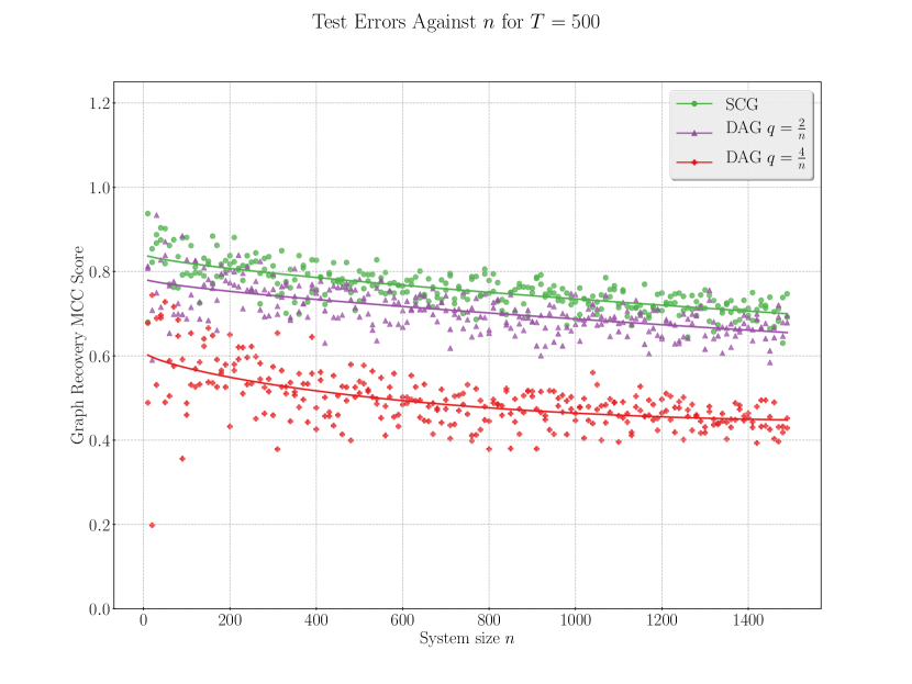
(a) Fixed $T$, increasing $n$ (SCG)

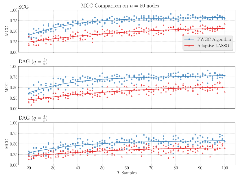
(b) MCC Comparison for $T\leq 100$

Figure 8(a) measures support recovery performance as the number of nodes $n$ increases, and the edge proportion as well as the number of samples $T$ is held fixed. Remarkably, the degradation as $n$ increases is limited, it is primarily the graph topology (SCG or non-SCG) as well as the level of sparsity (measured by $q$) which are the determining factors for support recovery performance.

Figure 8(b) provides a support recovery comparison for very small values of, $T$ typical for many applications.

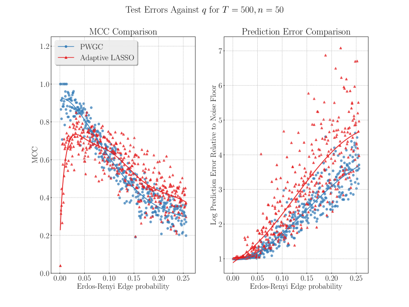
Figure 9: Fixed $T,n$, increasing edges $q$ (DAG)

Figure 9 provides a comparison between PWGC and AdaLASSO as the density of graph edges (as measured by $q$) increases. For reference, $\frac{2}{n}=0.04$ has approximately the same level of sparsity as the SCGs we simulated. As $q$ increases, the AdaLASSO outperforms PWGC as measured by the MCC. However, PWGC maintains superior performance for 1-step-ahead prediction. We speculate that this is a result of fitting the sparsity pattern recovered by PWGC via OLS which directly seeks to optimize this metric, whereas the LASSO is encumbered by the sparsity inducing penalty.

In reference to Figure 6 it should not be overly surprising that our PWGC algorithm performs better than the LASSO for the case of a strongly causal graph, since in this case the theory from which our heuristic derives is valid. However, the performance is still markedly superior in the case of a more general DAG. We would conjecture that a DAG having a similar degree of sparsity as an SCG is “likely” to be “close” to an SCG, in some appropriate sense.

Figure 9 illustrates the severe (expected) degradation in performance as the number of edges increases while the number of data samples $T$ remains fixed. For larger values $q$ in this plot, the number of edges in the graph is comparable to the number of data samples.

We have also paid close attention to the performance of PWGC in the very small sample ($T\leq 100$) regime (see Figure 8(b)), as this is the regime many applications must contend with.

In regards scalability, we have observed that performing the $O(n^{2})$ pairwise Granger causality calculations consumes the vast majority ($>90\%$) of the computation time. Since this step is trivially parallelizable, our algorithm also scales well with multiple cores or multiple machines. Figure 8(a) is a demonstration of this scalability, where we are able to estimate graphs having over $1500$ nodes (over $2.25\times 10^{6}$ possible edges) using only $T=500$ data points, granted, an SCG on this many nodes is extremely sparse.

References

- [1] C… Granger “Investigating Causal Relations by Econometric Models and Cross-spectral Methods” In Econometrica 37.3 [Wiley, Econometric Society], 1969, pp. 424–438 URL: http://www.jstor.org/stable/1912791
- [2] C.W.J. Granger “Testing for causality: A personal viewpoint” In Journal of Economic Dynamics and Control 2, 1980, pp. 329–352 DOI: http://dx.doi.org/10.1016/0165-1889(80)90069-X
- [3] Steven L Bressler and Anil K Seth “Wiener–Granger causality: a well established methodology” In Neuroimage 58.2 Elsevier, 2011, pp. 323–329
- [4] Anna Korzeniewska et al. “Dynamics of event-related causality in brain electrical activity” In Human Brain Mapping 29.10 Wiley Subscription Services, Inc., A Wiley Company, 2008, pp. 1170–1192 DOI: 10.1002/hbm.20458
- [5] Olivier David et al. “Identifying neural drivers with functional MRI: an electrophysiological validation” In PLoS Biol 6.12 Public Library of Science, 2008, pp. e315 URL: http://journals.plos.org/plosbiology/article?id=10.1371/journal.pbio.0060315
- [6] Monica Billio, Mila Getmansky, Andrew W. Lo and Loriana Pelizzon “Econometric Measures of Systemic Risk in the Finance and Insurance Sectors”, Working Paper Series 16223, 2010 DOI: 10.3386/w16223
- [7] André Fujita et al. “Modeling gene expression regulatory networks with the sparse vector autoregressive model” In BMC Systems Biology 1.1, 2007, pp. 39 DOI: 10.1186/1752-0509-1-39
- [8] Phan Nguyen “Methods for Inferring Gene Regulatory Networks from Time Series Expression Data” Copyright - Database copyright ProQuest LLC; ProQuest does not claim copyright in the individual underlying works; Last updated - 2019-05-11 In ProQuest Dissertations and Theses, 2019, pp. 175 URL: http://search.proquest.com.proxy.lib.uwaterloo.ca/docview/2205046162?accountid=14906
- [9] Aurélie C Lozano, Naoki Abe, Yan Liu and Saharon Rosset “Grouped graphical Granger modeling for gene expression regulatory networks discovery” In Bioinformatics 25.12 Oxford University Press, 2009, pp. i110–i118
- [10] Ali Shojaie and George Michailidis “Discovering graphical Granger causality using the truncating lasso penalty” In Bioinformatics 26.18, 2010, pp. i517–i523 DOI: 10.1093/bioinformatics/btq377
- [11] Michail Misyrlis, Rajgopal Kannan, Charalampos Chelmis and Viktor K. Prasanna “Sparse Causal Temporal Modeling to Inform Power System Defense” Complex Adaptive Systems Los Angeles, {CA} November 2-4, 2016 In Procedia Computer Science 95, 2016, pp. 450–456 DOI: http://dx.doi.org/10.1016/j.procs.2016.09.316
- [12] Tao Yuan and S Joe Qin “Root cause diagnosis of plant-wide oscillations using Granger causality” In Journal of Process Control 24.2 Elsevier, 2014, pp. 450–459
- [13] Trevor Hastie, Robert Tibshirani and Ryan J Tibshirani “Extended comparisons of best subset selection, forward stepwise selection, and the lasso” In arXiv preprint arXiv:1707.08692, 2017
- [14] Francis R Bach and Michael I Jordan “Learning graphical models for stationary time series” In IEEE transactions on signal processing 52.8 IEEE, 2004, pp. 2189–2199
- [15] Robert Tibshirani “Regression shrinkage and selection via the lasso” In Journal of the Royal Statistical Society: Series B (Methodological) 58.1 Wiley Online Library, 1996, pp. 267–288
- [16] Martin J Wainwright “Sharp thresholds for High-Dimensional and noisy sparsity recovery using l1-Constrained Quadratic Programming (Lasso)” In IEEE transactions on information theory 55.5 IEEE, 2009, pp. 2183–2202
- [17] Sumanta Basu and George Michailidis “Regularized estimation in sparse high-dimensional time series models” In Ann. Statist. 43.4 The Institute of Mathematical Statistics, 2015, pp. 1535–1567 DOI: 10.1214/15-AOS1315
- [18] Kam Chung Wong, Zifan Li and Ambuj Tewari “Lasso Guarantees for Time Series Estimation Under Subgaussian Tails beta-Mixing” In arXiv preprint arXiv:1602.04265, 2016
- [19] Y. Nardi and A. Rinaldo “Autoregressive process modeling via the Lasso procedure” In Journal of Multivariate Analysis 102.3, 2011, pp. 528–549 DOI: https://doi.org/10.1016/j.jmva.2010.10.012
- [20] David Hallac, Youngsuk Park, Stephen P. Boyd and Jure Leskovec “Network Inference via the Time-Varying Graphical Lasso” In CoRR abs/1703.01958, 2017 arXiv: http://arxiv.org/abs/1703.01958
- [21] Stefan Haufe, Klaus-Robert Müller, Guido Nolte and Nicole Krämer “Sparse causal discovery in multivariate time series” In Proceedings of the 2008th International Conference on Causality: Objectives and Assessment-Volume 6, 2008, pp. 97–106 JMLR. org
- [22] Andrew Bolstad, Barry D Van Veen and Robert Nowak “Causal network inference via group sparse regularization” In IEEE transactions on signal processing 59.6 IEEE, 2011, pp. 2628–2641
- [23] Yuejia He, Yiyuan She and Dapeng Wu “Stationary-sparse causality network learning.” In Journal of Machine Learning Research 14.1, 2013, pp. 3073–3104
- [24] Hui Zou “The adaptive lasso and its oracle properties” In Journal of the American statistical association 101.476 Taylor & Francis, 2006, pp. 1418–1429
- [25] Gary Hak Fui Tam, Chunqi Chang and Yeung Sam Hung “Gene regulatory network discovery using pairwise Granger causality” In IET systems biology 7.5 IET, 2013, pp. 195–204
- [26] Datta Gupta, Syamantak “On MMSE Approximations of Stationary Time Series” UWSpace, 2014 URL: http://hdl.handle.net/10012/8143
- [27] Mónika Józsa, Mihály Petreczky and M Kanat Camlibel “Relationship Between Granger Noncausality and Network Graph of State-Space Representations” In IEEE Transactions on Automatic Control 64.3 IEEE, 2018, pp. 912–927
- [28] Lionel Barnett and Anil K Seth “Granger causality for state-space models” In Physical Review E 91.4 APS, 2015, pp. 040101
- [29] Monika Józsa “Relationship between Granger non-causality and network graph of state-space representations” University of Groningen, 2019
- [30] P. Caines and C. Chan “Feedback between stationary stochastic processes” In IEEE Transactions on Automatic Control 20.4, 1975, pp. 498–508 DOI: 10.1109/TAC.1975.1101008
- [31] Anders Lindquist and Giorgio Picci “Linear stochastic systems: A geometric approach to modeling, estimation and identification” Springer, 2015
- [32] Lionel Barnett, Adam B Barrett and Anil K Seth “Granger causality and transfer entropy are equivalent for Gaussian variables” In Physical review letters 103.23 APS, 2009, pp. 238701
- [33] Sisi Ma, Patrick Kemmeren, David Gresham and Alexander Statnikov “De-Novo Learning of Genome-Scale Regulatory Networks in S. cerevisiae” In PLOS ONE 9.9 Public Library of Science, 2014, pp. 1–20 DOI: 10.1371/journal.pone.0106479
- [34] Andrew Arnold, Yan Liu and Naoki Abe “Temporal causal modeling with graphical granger methods” In Proceedings of the 13th ACM SIGKDD international conference on Knowledge discovery and data mining, 2007, pp. 66–75 ACM
- [35] Brian W Matthews “Comparison of the predicted and observed secondary structure of T4 phage lysozyme” In Biochimica et Biophysica Acta (BBA)-Protein Structure 405.2 Elsevier, 1975, pp. 442–451
- [36] Davide Chicco “Ten quick tips for machine learning in computational biology” In BioData mining 10.1 BioMed Central, 2017, pp. 35
- [37] Larry Wasserman “All of statistics: a concise course in statistical inference” Springer Science & Business Media, 2013
- [38] Kevin P. Murphy “Machine Learning: A Probabilistic Perspective” The MIT Press, 2012
- [39] Helmut Lütkepohl “New introduction to multiple time series analysis” Springer Science & Business Media, 2005
- [40] Monson H Hayes “Statistical digital signal processing and modeling” John Wiley & Sons, 2009
- [41] James Durbin “The fitting of time-series models” In Revue de l’Institut International de Statistique 28.3 JSTOR, 1960, pp. 233–244
- [42] P. Whittle “On the fitting of multivariate autoregressions, and the approximate canonical factorization of a spectral density matrix” In Biometrika 50.1-2, 1963, pp. 129–134 DOI: 10.1093/biomet/50.1-2.129
- [43] Yoav Benjamini and Yosef Hochberg “Controlling the false discovery rate: a practical and powerful approach to multiple testing” In Journal of the Royal statistical society: series B (Methodological) 57.1 Wiley Online Library, 1995, pp. 289–300
- [44] Eric Jones, Travis Oliphant and Pearu Peterson “SciPy: Open source scientific tools for Python”, 2001 URL: http://www.scipy.org/
- [45] Fabian Pedregosa et al. “Scikit-learn: Machine learning in Python” In Journal of machine learning research 12.Oct, 2011, pp. 2825–2830
- [46] Aric Hagberg, Pieter Swart and Daniel S Chult “Exploring network structure, dynamics, and function using NetworkX”, 2008