A Thermodynamically Consistent Fractional Visco-Elasto-Plastic Model with Memory-Dependent Damage for Anomalous Materials

Abstract

We develop a thermodynamically consistent, fractional visco-elasto-plastic model coupled with damage for anomalous materials. The model utilizes Scott-Blair rheological elements for both visco- elastic/plastic parts. The constitutive equations are obtained through Helmholtz free-energy potentials for Scott-Blair elements, together with a memory-dependent fractional yield function and dissipation inequalities. A memory-dependent Lemaitre-type damage is introduced through fractional damage energy release rates. For time-fractional integration of the resulting nonlinear system of equations, we develop a first-order semi-implicit fractional return-mapping algorithm. We also develop a finite-difference discretization for the fractional damage energy release rate, which results into Hankel-type matrix-vector operations for each time-step, allowing us to reduce the computational complexity from $\mathcal{O}(N^{3})$ to $\mathcal{O}(N^{2})$ through the use of Fast Fourier Transforms. Our numerical results demonstrate that the fractional orders for visco-elasto-plasticity play a crucial role in damage evolution, due to the competition between the anomalous plastic slip and bulk damage energy release rates.

34A08, 74A45, 74D10, 74S20, 74N30.

1 Introduction

Accurate and predictive modeling of material damage and failure for a wide range of materials poses multi-disciplinary challenges on experimental detection, consistent physics-informed models and efficient algorithms. Material failure arises in mechanical and biological systems as a consequence of internal damage, characterized in the micro-scale by the presence and growth of discontinuities e.g., microvoids, microcracks and bond breakage. Continuum Damage Mechanics (CDM) treats such effects in the macroscale through a representative volume element (RVE) [31]. When loading plastic crystalline materials, an initial hardening stage is observed from motion, arresting and network formation of dislocations, which is later overwhelmed by damage mechanisms, e.g. multiplication of micro-cracks/voids, followed by their growth and coalescing, releasing bulk energy from the RVE. Classical CDM models were proposed and validated in the past decades to describe the mechanical degradation, e.g., of ductile, brittle, and hyperelastic materials [48, 30]. Particularly, Lemaitre’s ductile damage model [30, 31] has been extensively employed for plasticity and visco-plasticity modeling of ductile materials. In such models, developing proper damage potentials driven by the so-called damage energy release rate [31] is a critical step.

Modeling the standard-to-anomalous damage evolution for power-law materials has additional challenges due to the non-Gaussian processes occurring on fractal-like media. Fractional constitutive laws utilize Scott-Blair (SB) elements [5, 4] as rheological building blocks that model the soft material response as a power-law memory-dependent device, interpolating between purely elastic/viscous behavior. A mechanical representation of the SB element was developed by Schiessel [47], as a hierarchical, continuous “ladder-like" arrangement of canonical Hookean/Newtonian elements (see Figure 1). Later on, Schiessel [46] generalized several standard visco-elastic models (Kelvin-Voigt, Maxwell, Kelvin-Zener, Poynting-Thompson) to their fractional counterparts by fully replacing the canonical elements with SB elements. Of particular interest, Lion [33] proved the thermodynamic consistency of the SB element from a mechanically-based fractional Helmholtz free-energy density.

With particular arrangements of SB and standard elements, fractional models were applied, e.g., to describe the far from equilibrium power-law dynamics of multi-fractional visco-elastic [26, 37, 40, 23, 38, 39], distributed visco-elastic [17] and visco-elasto-plastic [50, 54, 59, 25, 51] complex materials. Concurrently, significant advances in numerical methods allowed numerical solutions to time- and space- fractional partial differential equations (FPDEs) for smooth/non-smooth solutions, such as finite-difference (FD) schemes [34, 32], fractional Adams methods [16, 60], implicit-explicit (IMEX) schemes [11, 63], spectral methods [44, 45], fractional subgrid-scale modeling [43], fractional sensitivity equations [29], operator-based uncertainty quantification [28] and self-singularity-capturing approaches [53].

Despite the significant contributions on fractional constitutive laws, few works incorporated damage mechanisms. Zhang et al. [62] developed a nonlinear, visco-elasto-plastic creep damage model for concrete, where the damage evolution was defined through an exponential function of time. A similar model was proposed by Kang et al. [27] and applied to coal creep. Caputo and Fabrizio [12] developed a variable order visco-elastic model, where the variable order was regarded as a phase-field driven damage. Alfano and Musto [2] developed a cohesive zone, damaged fractional Kelvin-Zener model, and studied the influence of Hooke/SB damage energy release rates on damage evolution, motivating further studies on crack propagation mechanisms in visco-elastic media. Tang et al. [55] developed a variable order rock creep model, with damage evolution as an exponential function of time. Recently, Giraldo-Londoño et al. [22] developed a two-parameter, two-dimensional (2-D) rate-dependent cohesive fracture model.

A key aspect to develop failure models relies on consistent forms of damage energy release rates, usually appearing in the material-specific form of Helmholtz free-energy densities. For standard materials, direct summations of elastic/hyperelastic free-energies of the system are used. However, such process is non-trivial when modeling anomalous materials, due to the intrinsic mixed elasticity/viscosity of SB elements. Fabrizio [20] introduced a Graffi-Volterra free-energy for fractional models, but defined it without sufficient physical justification. Deseri et al. [15] developed free-energies for fractional hereditary materials, with the notion of order-dependent elasto-viscous and visco-elastic behaviors. Lion [33] derived the isothermal Helmholtz free-energy density for SB elements using a discrete-to-continuum arrangement of standard Maxwell branches, and employed it in the Clausius-Duhem inequality to obtain the stress-strain relationship. Later on, Adolfsson et al. [1] employed Lion’s approach to prove the thermodynamic admissibility of the SB constitutive law written as a Volterra integral equation of first kind.

To the authors’ best knowledge, only Alfano and Musto [2] coupled the fractional free-energy density to a damage evolution equation in viscoelasticity, but fractional extensions of (non-exponential) damage for visco-elasto-plastic materials are still lacking. In addition, for damage models, efficient numerical methods for fractional free-energy computations are also virtually nonexistent in the literature. A numerical approximation was done by Burlon et al. [9], through a finite summation of free-energies from Hookean elements, which is a truncation of the infinite number of relaxation modes carried by the fractional operators. Alfano and Musto [2] briefly described how to discretize the SB free-energy using a midpoint finite-difference scheme. A few numerical results were presented for damage evolution, but the authors did not describe the discretizations and no accuracy is investigated for the numerical scheme.

In this work we develop a thermodynamically consistent, one-dimensional (1-D) fractional visco-elasto-plastic model with memory-dependent damage in the context of CDM. The main characteristics of the model follow:

• We employ SB elements in both visco-elastic and visco-plastic parts, respectively, with orders $\beta_{E},\beta_{K}\in(0,1)$, leading to power-law effects in both ranges.

• The damage reduces the total free-energy of the model, while constitutive laws are obtained through the Clausius-Duhem inequality.

• The yield function is time-fractional rate-dependent, while the damage potential is Lemaitre-like. The damage energy release rate is taken as the SB Helmholtz free-energy density to describe the anomalous bulk energy loss.

• We prove the positive dissipation, and therefore the thermodynamic consistency of the developed model (see Theorem 4.5).

Since obtaining analytical solutions for the resulting nonlinear system of multi-term visco-elasto-plastic fractional differential equations (FDEs) coupled with damage is cumbersome or even impossible, we performed an efficient time-integration framework as follows:

• We develop a first-order, semi-implicit fractional return-mapping algorithm, with explicit evaluation of damage in the stress-strain relationship and yield function. An implicit FD scheme is employed to the ODEs for plastic and damage variables. The time-fractional stress-strain relationship and yield function are discretized using the L1 FD scheme from Lin and Xu [32].

• We develop a fully-implicit scheme for the SB Helmholtz free-energy density, and hence to the fractional damage energy release rate. We then exploit the structure of the discretized energy and apply Fast Fourier Transforms (FFTs) to obtain an efficient scheme.

• The accuracy of free-energy discretization is proved to be of order $\mathcal{O}(\Delta t^{2-\beta})$, and numerical tests show a computational complexity of order $\mathcal{O}(N^{2}\log N)$, with N being the number of time-steps.

The developed fractional return-mapping algorithm can be easily incorporated to existing finite element (FE) frameworks as a constitutive box. Numerical tests are performed with imposed monotone and cyclic strains, and demonstrate that:

• Softening, hysteresis and low-cycle fatigue can be modeled.

• Memory-dependent damage energy release rates induce anomalous damage evolutions with competing visco-elastic/plastic effects, without changing the form of Lemaitre’s damage potential.

The developed model motivates applications to failure of biological materials [7], where micro-structural evolution can be upscaled to the continuum through evolving fractional orders $\beta_{E}$, $\beta_{K}$ [36] and damage $D$. The memory-dependent fractional damage energy release rates motivate studies on anomalous bulk-to-surface energy loss in damage accumulation/crack propagation of, e.g., bone tissue, where intrinsic/extrinsic plasticity/crack-bridging mechanisms [58] lead to a complex nature of failure.

This work is organized as follows: In Section 2 we present definitions of fractional operators. In Section 3, we present the thermodynamics and rheology of SB elements. In Section 4, we develop the fractional visco-elasto-plastic model with damage, followed by its discretization. A series of numerical tests are shown in Section 5, followed by discussions and concluding remarks in Section 6.

2 Definitions of Fractional Calculus

We start with some preliminary definitions of fractional calculus [41]. The left-sided Riemann-Liouville integral of order $\beta\in(0,1)$ is defined as

(1) $$(\prescript{RL}{t_{L}}{\mathcal{I}}_{t}^{\beta}f)(t)=\frac{1}{\Gamma(\beta)}\int_{t_{L}}^{t}\frac{f(s)}{(t-s)^{1-\beta}}\,ds,\,\,\,\,\,\,t>t_{L},$$

where $\Gamma$ represents the Euler gamma function and $t_{L}$ denotes the lower integration limit. The corresponding inverse operator, i.e., the left-sided fractional derivative of order $\beta$, is then defined based on (1) as

$$(\prescript{RL}{t_{L}}{\mathcal{D}}_{t}^{\beta}f)(t)=\frac{d}{dt}(\prescript{RL}{t_{L}}{\mathcal{I}}_{t}^{1-\beta}f)(t)=\frac{1}{\Gamma(1-\beta)}\frac{d}{dt}\int_{t_{L}}^{t}\frac{f(s)}{(t-s)^{\beta}}\,ds,\,\,\,\,\,\,t>t_{L}.$$

Also, the left-sided Caputo derivative of order $\beta\in(0,1)$ is obtained as

$$(\prescript{C}{t_{L}}{\mathcal{D}}_{t}^{\beta}f)(t)=(\prescript{RL}{t_{L}}{\mathcal{I}}_{t}^{1-\beta}\frac{df}{dt})(t)=\frac{1}{\Gamma(1-\beta)}\int_{t_{L}}^{t}\frac{f^{\prime}(s)}{(t-s)^{\beta}}\,ds,\,\,\,\,\,\,t>t_{L}.$$

The definitions of Riemann-Liouville and Caputo derivatives are linked by the following relationship:

$$(\prescript{RL}{t_{L}}{\mathcal{D}}_{t}^{\beta}f)(t)=\frac{f(t_{L})}{\Gamma(1-\beta)(t+t_{L})^{\beta}}+(\prescript{C}{t_{L}}{\mathcal{D}}_{t}^{\beta}f)(t),$$

which denotes that the definition of the aforementioned derivatives coincide when dealing with homogeneous Dirichlet initial/boundary conditions.

2.1 Interpretation of Caputo derivatives in terms of nonlocal vector calculus

In this section we show that the Caputo derivative can be reinterpreted as the limit of a nonlocal truncated time derivative [19]. This fact establishes a connection between nonlocal initial value problems and their fractional counterparts, which can benefit from the nonlocal theory.

Given a nonnegative and symmetric kernel function $\rho_{\delta}(s)=\rho_{\delta}(|s|)$, a nonlocal, weighted, gradient operator can be defined as [18]

(2) $$\mathcal{G}_{\delta}f(t)=\lim\limits_{\epsilon\to 0}\displaystyle\int_{\epsilon}^{\delta}(f(t)-f(t-s))s\rho_{\delta}(s)\,ds,$$

when the limit exists in $L^{2}(0,T)$ for a function $f\in L^{2}(0,T)$. It is common to assume that the kernel function $\rho_{\delta}$ has compact support in $[-\delta,\delta]$ and a normalized moment:

(3) $$\int_{0}^{\delta}s^{2}\rho_{\delta}(s)\,ds=1.$$

Here, the parameter $\delta>0$ represents the extent of the nonlocal interactions or, in case of time dependence, the memory span. In the nonlocal theory it is usually referred to as horizon.

Note that at the limit of vanishing nonlocality, i.e. as $\delta\to 0$, $\mathcal{G}_{\delta}$ corresponds to the classical first order time derivative operator $\frac{d}{dt}$. In this work, we are interested in the limit of infinite interactions, i.e. as $\delta\to\infty$. Specifically, when the initial data $f(t):=f(0)$ for all $t\in(-\infty,0)$ and the kernel function is defined as

(4) $$\rho_{\infty}(s)=\dfrac{\beta}{\Gamma(1-\beta)}s^{-\beta-2},\quad{\rm for}\;\beta\in(0,1),$$

the nonlocal operator $\mathcal{G}_{\delta}$ corresponds to the Caputo fractional derivative for $t>0$, for a piecewise differentiable function $f\in C(-\infty,T)$ such that $f^{\prime}\in L^{1}(0,T)\cap C(0,T]$. Formally,

(5) $$\mathcal{G}_{\infty}f(t)=(\prescript{C}{0}{\mathcal{D}}_{t}^{\beta}f)(t).$$

Note that a similar property holds true for fractional derivatives in space, see [14].

2.1.1 Note on well-posedness

Paper [19] analyzes the well-posedness of nonlocal initial value problems. More specifically, it proves, under certain conditions on the parameters, that the following equation has a unique solution and depends continuously upon the data.

(6) $$\mathcal{G}_{\delta}\gamma+H\gamma =F \;\;t\in(0,T],$$

$$\gamma =G \;\;t\in(-\delta,0),$$

for $H>0$ and $F$ and $G$ in suitable functional spaces.

3 Thermodynamics of Fractional Scott-Blair Elements

We present the thermodynamic principles used in this work, and then we introduce the Helmholtz free-energy density and constitutive law for the fractional SB element. Such fractional element is the rheological building block of our modeling approach, providing a constitutive interpolation between a Hookean $(\beta\to 0)$ and Newtonian $(\beta\to 1)$ element (see Figure 1). Furthermore, the SB element can be interpreted as an infinite self-similar arrangement of standard Maxwell elements, which naturally leads to fractional operators in the constitutive law [47].

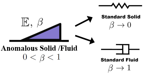
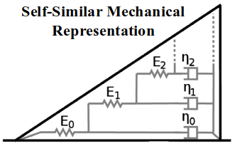
Figure 1: (left) Schematics of the SB element recovering standard limit cases. (right) The SB element seen as an infinite, hierarchical mechanical representation of canonical elements, coding an infinite number of relaxation times. The pair $(\mathbb{E},\beta)$ represents a dynamic process of the material.

3.1 Thermodynamic Principles

Let a closed system undergo an irreversible, isothermal, strain-driven thermodynamic process. We analyze an infinitesimal material region at a position $x$ and time $t$ of a continuum deformable body $\mathcal{B}$. Let the first law of thermodynamics in rate form [3] be defined as:

(7) $$\dot{e}=\dot{q}-\dot{w},$$

where $\dot{e}(x,t)$ $[J.s^{-1}.kg^{-1}]$ denotes the specific rate of internal energy, the term $\dot{q}(x,t)$ $[J.s^{-1}.kg^{-1}]$ represents the rate of specific heat exchange, and $\dot{w}(x,t)$ $[J.s^{-1}.kg^{-1}]$ denotes the stress power transferred into the bulk due to external forces [24]. In this work, $\tau(x,t)$ represents the stress state and $\dot{\varepsilon}$ the strain rate. We also consider the second law of thermodynamics, postulating the irreversibility of entropy production, given, in specific form, by:

(8) $$\dot{s}\geq\dot{q}/\theta,$$

where $\dot{s}(x,t)\,[J.s^{-1}.kg^{-1}.K^{-1}]$ denotes the rate of specific entropy production and $\theta(x,t)=\theta_{0}\,[K]$ represents the constant temperature. Let $\psi(x,t):\mathbb{R}\times\mathbb{R}^{+}\to\mathbb{R}^{+}$ be the Helmholtz free-energy density with units $[J.m^{-3}]$, representing the available energy to perform work, defined by $\psi:=\rho\left(e-\theta s\right)$, with the rate form $\dot{\psi}=\rho\left(\dot{e}-\theta\dot{s}\right)$ for the isothermal case. Combining the first and second laws, respectively, (7) and (8), with $\dot{\psi}$ and taking the stress power $\dot{w}=-\tau\dot{\varepsilon}$, we obtain the Clausius-Duhem inequality, which states the non-negative dissipation rates [13]:

(9) $$-\dot{\psi}+\tau\dot{\varepsilon}\geq 0,\quad\forall x\in\mathcal{B}.$$

Satisfying the dissipation inequality (9) is here taken as the necessary condition for the potential $\psi$ and the stress $\tau$ to be thermodynamically admissible.

3.2 Helmholtz Free-Energy Density

We present the free-energy under consideration for the employed SB element, here referred to a given material coordinate of a continuum body or a lumped mechanical system. We start with the fractional Helmholtz free-energy density developed by Lion [33], obtained through an integration of a continuum spectrum of Maxwell branches leading to the following definition for $\psi(\varepsilon):\mathbb{R}\to\mathbb{R}^{+}$:

(10) $$\psi(\varepsilon)=\frac{1}{2}\int^{\infty}_{0}\tilde{E}(z)\left[\int^{t}_{0}\exp\left(-\frac{t-s}{z}\right)\dot{\varepsilon}(s)\,ds\right]^{2}\,dz,$$

where we the strain $\varepsilon$ is taken as the state variable. The term $\tilde{E}(z):\mathbb{R}^{+}\to\mathbb{R}^{+}$ denotes the power-law relaxation spectrum, given by

$$\tilde{E}(z)=\frac{\mathbb{E}}{\Gamma(1-\beta)\Gamma(\beta)z^{\beta+1}},\quad 0<\beta<1,\quad\mathbb{E}\in\mathbb{R}^{+},$$

which with (10), codes an infinite number of relaxation times. The pseudo-constant $\mathbb{E}$ has units $[Pa.s^{\beta}]$, where the unique pair $(\mathbb{E},\beta)$ codes a dynamic process instead of an equilibrium state of the material [26]. Let $\mathcal{D}_{mech}$ denote the mechanical dissipation of the SB element. We introduce the following Lemmas:

Lemma 3.1.

The SB element stress-strain relationship $\tau(t):\mathbb{R}^{+}\to\mathbb{R}$ resulting from (10) and the Clausius-Duhem inequality (9) is given by

(11) $$\tau(t)=\int^{\infty}_{0}\tilde{E}(z)\left(\int^{t}_{0}\exp\left(-\frac{t-s}{z}\right)\dot{\varepsilon}(s)\,ds\right)\,dz=\mathbb{E}\,{}^{C}_{0}\mathcal{D}^{\beta}_{t}\varepsilon(t),$$

where the Caputo definition for the fractional derivative is a consequence of the adopted free-energy. The mechanical dissipation $\mathcal{D}_{mech}(\varepsilon):\mathbb{R}\to\mathbb{R}^{+}$ for the SB element is given by the following form:

(12) $$\mathcal{D}_{mech}(\varepsilon)=\int^{\infty}_{0}\frac{\tilde{E}(z)}{z}\left(\int^{t}_{0}\exp\left(-\frac{t-s}{z}\right)\dot{\varepsilon}(s)\,ds\right)^{2}dz.$$

Proof 3.2.

See Appendix A.

Remark 3.3.

The limit cases for the fractional free-energy (10) with respect to $\beta$ are consistent with the well-known stress-strain relationship (11). Therefore, $\psi(\varepsilon)$ recovers a fully conserving Hookean spring when $\lim_{\beta\to 0}\psi=\mathbb{E}\varepsilon^{2}/2$, and a fully dissipative Newtonian dashpot when $\lim_{\beta\to 1}\psi=0$. We refer the readers to [33, 15] for additional details regarding memory-dependent free-energies.

4 Fractional Visco-Elasto-Plastic Model with Damage

We develop a damage formulation for a fractional visco-elasto-plastic model (M1) by Suzuki et al. [54]. The closure for the damage variable is obtained through a Lemaitre-type approach [30, 31]. We later prove the thermodynamic consistency of the damage model, and hence for the visco-elasto-plastic model (M1) as a limiting, undamaged case.

4.1 Thermodynamic Formulation

The fractional visco-elasto-plastic device is illustrated in Figure 2. It consists of a SB element with material pair $(\mathbb{E},\beta_{E})$ for the visco-elastic part, under a corresponding logarithmic visco-elastic strain $\varepsilon^{ve}(t):\mathbb{R}^{+}\to\mathbb{R}$. The visco-plastic part is given by a parallel combination of a Coulomb frictional element with yield stress $\tau^{Y}\,[Pa]\in\mathbb{R}^{+}$, a linear hardening Hooke element with constant $H\,[Pa]\in\mathbb{R}^{+}$, and a SB element with material pair $(\mathbb{K},\beta_{K})$, with $\mathbb{K}\,[Pa.s^{\beta_{K}}]\in\mathbb{R}^{+}$, all subject to a logarithmic visco-plastic strain $\varepsilon^{vp}(t):\mathbb{R}^{+}\to\mathbb{R}$ and an internal hardening variable $\alpha(t):\mathbb{R}^{+}\to\mathbb{R}^{+}$. The entire device is subject to a Kirchhoff stress $\tau$. The total logarithmic strain is given by:

(13) $$\varepsilon(t)=\varepsilon^{ve}(t)+\varepsilon^{vp}(t).$$

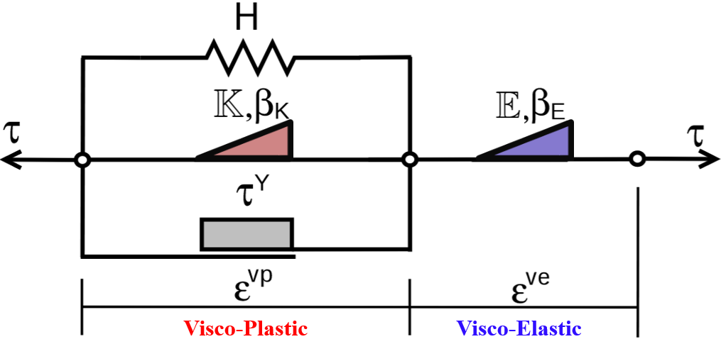
(a) Rheological diagram.

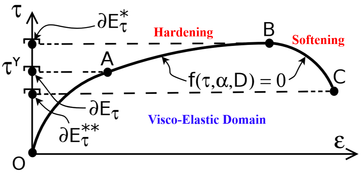
(b) Stress vs. strain response.

Figure 2: Damaged fractional visco-elasto-plastic model. (A) Constitutive diagram with visco-elastic/plastic rheological elements. (B) Stress response showing the yield surface expansion (hardening) and contraction (softening).

Let $D(t):\mathbb{R}^{+}\to\Omega_{D}$, with $\Omega_{D}=[0,1)$ be a time-dependent and monotonically increasing internal damage variable representing the internal material degradation. Our model has the following assumptions: The visco-elastic response is linear, under an isothermal strain-driven process. There is a state coupling between the visco-elastic strains/hardening variable $\varepsilon^{ve}$, $\alpha$, and damage $D$. However, the damage evolution is solely driven by the visco-elastic free-energy potential. There is no state coupling between visco-elasticity and visco-plasticity. The damage $D(t)$ and hardening $\alpha(t)$ are irreversible, i.e., there is no material healing. Also, there are no crack closure effects. All state and internal variables are subject to homogeneous initial conditions, e.g., $\varepsilon(0)=\varepsilon^{ve}(0)=\varepsilon^{vp}(0)=\alpha(0)=D(0)=0$.

Assumption (2) implies a linearity between the visco-elastic and visco-plastic free-energy components, both multiplicatively coupled with damage.

4.1.1 Free-Energy Densities

We write the Helmholtz free-energy density $\psi(\varepsilon^{ve},\,\alpha,\,D):\mathbb{R}\times\mathbb{R}^{+}\times\Omega_{D}\to\mathbb{R}^{+}$ for the model as:

(14) $$\psi(\varepsilon^{ve},\,\alpha,\,D)=\left(1-D\right)\left(\bar{\psi}^{ve}(\varepsilon^{ve})+\bar{\psi}^{vp}(\alpha)\right),$$

where $\bar{\psi}^{ve}(\varepsilon^{ve}):\mathbb{R}\to\mathbb{R}^{+}$ and $\bar{\psi}^{vp}(\alpha):\mathbb{R}^{+}\to\mathbb{R}^{+}$ represent the undamaged visco-elastic and visco-plastic free-energy densities. Utilizing (10) for the SB elements and the Hookean spring, the free-energy density is given by:

(15) $$\psi(\varepsilon^{ve},\alpha,\,D) =\frac{1}{2}\left(1-D\right)\left[\int^{\infty}_{0}\tilde{E}(z)\left(\int^{t}_{0}\exp\left(-\frac{t-s}{z}\right)\dot{\varepsilon}^{ve}(s)\,ds\right)^{2}\,dz\right.$$

$$\left.+\int^{\infty}_{0}\tilde{K}(z)\left(\int^{t}_{0}\exp\left(-\frac{t-s}{z}\right)\dot{\alpha}(s)\,ds\right)^{2}\,dz+H\alpha^{2}\right],$$

with the following relaxation spectra for visco-elasticity and visco-plasticity:

$$\tilde{E}(z)=\frac{\mathbb{E}}{\Gamma(1-\beta_{E})\Gamma(\beta_{E})z^{\beta_{E}+1}},\quad\tilde{K}(z)=\frac{\mathbb{K}}{\Gamma(1-\beta_{K})\Gamma(\beta_{K})z^{\beta_{K}+1}},$$

where $0<\beta_{E},\,\beta_{K}<1$.

Remark 4.1 (Recovery of classical free-energy potentials).

Similar to the SB element case, we recover the Hookean and Newtonian limit cases for the asymptotic values of $\beta_{E}$, $\beta_{K}$. Also, if $D\to 0$, we recover an undamaged case, and when $D\to 1$, we have $(1-D)\psi\to 0$ (material failure).

4.1.2 Constitutive Laws

We use the Clausius-Duhem inequality (9) in the local form of classical thermodynamics of internal variables, which induces near-equilibrium states for every time $t$ of the thermodynamic process. However, the fractional free-energy densities introduce memory effects and therefore far-from-equilibrium states in the scope of rational thermodynamics [20]. Using (14) and (13), inequality (9) is given by:

(16) $$-\rho\dot{\psi}(\varepsilon^{ve},\alpha,D)+\tau\left(\dot{\varepsilon}^{ve}+\dot{\varepsilon}^{vp}\right)\geq 0,$$

where we evaluate $\dot{\psi}$ as follows:

(17) $$\dot{\psi}(\varepsilon^{ve},\dot{\varepsilon}^{ve},\alpha,\dot{\alpha},D,\dot{D})=\frac{\partial\psi}{\partial\varepsilon^{ve}}\dot{\varepsilon}^{ve}+\frac{\partial\psi}{\partial\alpha}\dot{\alpha}+\frac{\partial\psi}{\partial D}\dot{D}.$$

Similar to the proof of Lemma 3.1, the partial derivatives are obtained by chain and Leibniz rules. For the first term on the RHS of (17), we have:

$$\frac{\partial\psi}{\partial\varepsilon^{ve}}\dot{\varepsilon}^{ve}= \left(1-D\right)\left[\int^{\infty}_{0}\tilde{E}(z)\left(\int^{t}_{0}\exp\left(-\frac{t-s}{z}\right)\dot{\varepsilon}^{ve}(s)\,ds\right)dz\,\dot{\varepsilon}^{ve}\right.$$

$$\left.-\int^{\infty}_{0}\frac{\tilde{E}(z)}{z}\left(\int^{t}_{0}\exp\left(-\frac{t-s}{z}\right)\dot{\varepsilon}^{ve}(s)\,ds\right)^{2}dz\right].$$

Recalling (12), we rewrite the above equation as:

(18) $$\frac{\partial\psi}{\partial\varepsilon^{ve}}\dot{\varepsilon}^{ve}= \left(1-D\right)\left[\int^{\infty}_{0}\tilde{E}(z)\left(\int^{t}_{0}\exp\left(-\frac{t-s}{z}\right)\dot{\varepsilon}^{ve}(s)\,ds\right)dz\,\dot{\varepsilon}^{ve}-\mathcal{D}^{ve}_{mech}(\varepsilon^{ve})\right],$$

where $\mathcal{D}^{ve}_{mech}(\varepsilon^{ve}):\mathbb{R}\to\mathbb{R}^{+}$ represents the visco-elastic mechanical energy dissipation, given by:

$$\mathcal{D}^{ve}_{mech}(\varepsilon^{ve})=\int^{\infty}_{0}\frac{\tilde{E}(z)}{z}\left(\int^{t}_{0}\exp\left(-\frac{t-s}{z}\right)\dot{\varepsilon}^{ve}(s)\,ds\right)^{2}dz.$$

Similarly, we obtain the second term on the RHS of (17):

(19) $$\frac{\partial\psi}{\partial\alpha}\dot{\alpha}=R(t)\dot{\alpha}-(1-D)\mathcal{D}^{vp}_{mech}(\alpha),$$

where $R(t):\mathbb{R}^{+}\to\mathbb{R}^{+}$ represents the accumulated stress acting on the SB and Hooke elements on the visco-plastic part due to the accumulated visco-plastic strains. Recalling Lemma 3.1, $R(t)$ reads:

$$R(t) =\left(1-D\right)\left[\int^{\infty}_{0}\tilde{K}(z)\left(\int^{t}_{0}\exp\left(-\frac{t-s}{z}\right)\dot{\alpha}(s)\,ds\right)dz+H\alpha\right]$$

$$=\left(1-D\right)\left[\mathbb{K}\,{}^{C}_{0}\mathcal{D}^{\beta_{K}}_{t}\left(\alpha\right)+H\alpha\right].$$

On the other hand, the term $\mathcal{D}^{vp}_{mech}(\alpha):\mathbb{R}^{+}\to\mathbb{R}^{+}$ denotes the visco-plastic mechanical energy dissipation in the model, which is given by:

$$\mathcal{D}^{vp}_{mech}(\alpha)=\int^{\infty}_{0}\frac{\tilde{K}(z)}{z}\left(\int^{t}_{0}\exp\left(-\frac{t-s}{z}\right)\dot{\alpha}(s)\,ds\right)^{2}dz.$$

Finally, the direct calculation of the last term on the RHS of (17) yields:

(20) $$\frac{\partial\psi}{\partial D}\dot{D}=\left[Y^{ve}(\varepsilon^{ve})+Y^{vp}(\alpha)\right]\dot{D}=Y(\varepsilon^{ve},\alpha)\dot{D},$$

where $Y^{ve}(\varepsilon^{ve}):\mathbb{R}\to\mathbb{R}^{-}$ and $Y^{vp}(\alpha):\mathbb{R}^{+}\to\mathbb{R}^{-}$ denote, respectively, the visco-elastic/plastic damage energy release rates. From (14), they are respectively given by:

(21) $$Y^{ve}(\varepsilon^{ve})=-\bar{\psi}^{ve}(\varepsilon^{ve})=-\frac{1}{2}\int^{\infty}_{0}\tilde{E}(z)\left(\int^{t}_{0}\exp\left(-\frac{t-s}{z}\right)\dot{\varepsilon}^{ve}(s)\,ds\right)^{2}dz.$$

(22) $$Y^{vp}(\alpha)=-\bar{\psi}^{vp}(\alpha)=-\frac{1}{2}\int^{\infty}_{0}\tilde{K}(z)\left(\int^{t}_{0}\exp\left(-\frac{t-s}{z}\right)\dot{\alpha}(s)\,ds\right)^{2}dz.$$

We observe from the above result that, in principle, both visco-elastic and visco-plastic parts release bulk energy with respect to damage. Inserting (18), (19) and (20) into (16), recalling Lemma 3.1, and dropping the function variables, we obtain:

(23) $$\left[\tau-\left(1-D\right)\mathbb{E}\,{}^{C}_{0}\mathcal{D}^{\beta_{E}}_{t}\left(\varepsilon^{ve}\right)\right]\dot{\varepsilon}^{ve} +\tau\dot{\varepsilon}^{vp}-R\dot{\alpha}$$

$$-Y\dot{D}+(1-D)\left(\mathcal{D}^{ve}_{mech}+\mathcal{D}^{vp}_{mech}\right)\geq 0.$$

Since the strain rate $\dot{\varepsilon}^{ve}$ in (23) is arbitrary, without violating the inequality, we can set its multiplying argument to zero, and obtain the following stress-strain relationship:

(24) $$\tau(t)=\left(1-D\right)\mathbb{E}\,{}^{C}_{0}\mathcal{D}^{\beta_{E}}_{t}\left(\varepsilon^{ve}\right),$$

and alternatively, using (13), we obtain:

(25) $$\tau(t)=\left(1-D\right)\mathbb{E}\,{}^{C}_{0}\mathcal{D}^{\beta_{E}}_{t}\left(\varepsilon-\varepsilon^{vp}\right),$$

and hence, the total energy dissipation (23) becomes:

(26) $$\tau\dot{\varepsilon}^{vp}-R\dot{\alpha}-Y\dot{D}+(1-D)\left(\mathcal{D}^{ve}_{mech}+\mathcal{D}^{vp}_{mech}\right)\geq 0.$$

Hence, we obtained the stress-strain relationships and dissipation potentials.

4.1.3 Evolution Laws for Visco-Plasticity and Damage

In order to obtain the kinematic equations for the internal variables, we define a combined hardening and damage dissipation potential $F\left(\tau,\alpha,Y,D\right):\mathbb{R}\times\mathbb{R}^{+}\times\mathbb{R}^{-}\times\mathbb{R}^{+}\to\mathbb{R}$, in the form [30, 31]:

(27) $$F\left(\tau,\alpha,Y,D\right):=f\left(\tau,\alpha,D\right)+F_{D}\left(Y^{ve},D\right),$$

where $f\left(\tau,\alpha,D\right):\mathbb{R}\times\mathbb{R}^{+}\times\mathbb{R}^{+}\to\mathbb{R}^{-}\cup\{0\}$ represents a yield function, defined here as the difference between the absolute value of the applied stress in the device and the stress acting on the visco-plastic part [54]:

$$f\left(\tau,\alpha,D\right) :=\lvert\tau\rvert-\left[(1-D)\tau^{Y}+R\right]$$

(28) $$=\lvert\tau\rvert-\left(1-D\right)\left[\tau^{Y}+\mathbb{K}\,{}^{C}_{0}\mathcal{D}^{\beta_{K}}_{t}\left(\alpha\right)+H\alpha\right],$$

which softens the visco-plastic stresses.

Lemma 4.2.

The set of admissible stresses lies in a closed convex space (see Fig.2) with respect to the associated thermodynamic variables $\tau$ and $R$ [31], given by:

(29) $$E_{\tau}=\{\tau\in\mathbb{R}|f(\tau,\alpha,D)<0\}.$$

The boundary of $E_{\tau}$, denoted by $\partial E_{\tau}$, is the convex set given by:

$$\partial E_{\tau}=\{\tau\in\mathbb{R}|f(\tau,\alpha,D)=0\},$$

where $f(\tau,\alpha,D)=0$ denotes the yield condition in classical plasticity.

Proof 4.3.

See Appendix C.

The term $F_{D}\left(Y^{ve},D\right):\mathbb{R}^{-}\times\mathbb{R}^{+}\to\mathbb{R}^{+}$ represents a damage potential driven by the plastic strains and visco-elastic free-energy (see Assumption 2), where we adopt Lemaitre’s form for ductile materials [31]:

(30) $$F_{D}(Y,D):=\frac{S}{(s+1)(1-D)}\left(-\frac{Y^{ve}}{S}\right)^{s+1},$$

where $S\in\mathbb{R}^{+}$ $[Pa]$ and $s\in\mathbb{R}^{+}$ represent material parameters, identified, e.g., by Cao et al. [10] for a Zirconium alloy, and by Bouchard et al. [8] for highly ductile metals. In the latter, an inverse power-law form for $F_{D}$ was defined with respect to the equivalent plastic strains to avoid damage over-estimation. The sensitivity of Lemaitre’s model with respect to $S$ and $s$ was studied by Roux and Bouchard [42].

From the defined yield function (4.1.3), and the principle of maximum plastic dissipation [49], the following properties hold: i) associativity of the flow rule, ii) associativity in the hardening law, iii) Kuhn-Tucker complimentary conditions, and iv) convexity of $E_{\tau}$. Therefore, we obtain a set of evolution equations for $\varepsilon^{vp}$, $\alpha$ and $D$:

$$\dot{\varepsilon}^{vp}=\frac{\partial f}{\partial\tau}\dot{\gamma},\quad\dot{\alpha}=-\frac{\partial f}{\partial R}\dot{\gamma},\quad\dot{D}=-\frac{\partial F_{D}}{\partial Y^{ve}}\dot{\gamma},$$

where $\dot{\gamma}(t):\mathbb{R}^{+}\to\mathbb{R}^{+}$ denotes the plastic slip rate. For simplicity, we consider only variations of the potential $F_{D}$ with respect to the free-energy from the visco-elastic component for the damage evolution. Evaluating the above equations using (4.1.3) and (30), we obtain, respectively, the evolution for visco-plastic strains, hardening variable, and damage:

(31) $$\dot{\varepsilon}^{vp}=\mathrm{sign}(\tau)\dot{\gamma},$$

(32) $$\dot{\alpha}=\dot{\gamma},$$

(33) $$\dot{D}=\frac{\dot{\gamma}}{(1-D)}\left(-\frac{Y^{ve}}{S}\right)^{s},$$

where the first two evolution laws coincide with the ones defined for the model M1 by Suzuki et al. [54] for fractional visco-elasto-plasticity.

Remark 4.4.

The obtained nonlinear damage evolution (33) coincides with local Lemaitre’s form [30, 31]. However, due to the time-fractional form of $Y^{ve}$, power-law memory effects for damage are introduced in the model.

Theorem 4.5 (Positive dissipation).

The mechanical dissipation for the damaged, fractional visco-elasto-plastic model is positive and given by,

$$\left(1-D(t)\right)\left[\tau^{Y}\dot{\gamma}(t)+\mathcal{D}^{ve}_{mech}(\varepsilon^{ve})+\mathcal{D}^{vp}_{mech}(\alpha)\right]-Y(\varepsilon^{ve},\alpha)\dot{D}(t)\geq\,0,$$

where the above Clausius-Duhem inequality holds. Therefore, the defined Helmholtz free-energy density (15), the obtained stress-strain relationship (25) and evolution equations (31)-(33) of the developed model are thermodynamically admissible.

Proof 4.6.

See Appendix B.

4.2 Time-Fractional Integration

We develop two new algorithms for time-fractional integration of the developed model. The first one is a semi-implicit fractional return-mapping algorithm, that can be implemented in zero- or one- dimensional systems as a constitutive box. The second one is an FD discretization for the fractional Helmholtz free-energy density and damage energy release rate $Y$ (21). Let $t\in(0,T]$, and an uniform time grid given by $t_{n}=n\Delta t$, with $n=0,\,1,\,\dots,\,N$ and time-step size $\Delta t=T/N$.

4.2.1 Semi-Implicit Fractional Return-Mapping Algorithm

We employ a backward-Euler scheme considering all variables to be implicit, except the damage $D$ in the stress-strain relationship and yield function. We refer the readers to [8] for a comparison between implicit/semi-implicit integer-order return-mapping algorithms. Such explicit treatment of $D$ weakly couples the damage and plastic slip, simplifying the visco-plastic time-integration. Given known total strains $\varepsilon_{n}$ at time $t_{n}$, and a strain increment $\Delta\varepsilon_{n+1}$ we have $\varepsilon_{n+1}=\varepsilon_{n}+\Delta\varepsilon_{n+1}$. The discrete form of the stress-strain relationship (25) reads:

(34) $$\tau_{n+1}=(1-D_{n})\mathbb{E}\,{}^{C}_{0}\mathcal{D}^{\beta_{E}}_{t}\left(\varepsilon-\varepsilon^{vp}\right)\big{|}_{t=t_{n+1}}.$$

The backward-Euler discretization of the flow rule (31) yields:

(35) $$\varepsilon^{vp}_{n+1}=\varepsilon^{vp}_{n}+\operatorname{\mathrm{sign}}(\tau_{n+1})\Delta\gamma,$$

with $\Delta\gamma=\gamma_{n+1}-\gamma_{n}$ representing the plastic slip increment in the interval $[t_{n},\,t_{n+1}]$. Similarly, the discretization of the hardening law (32) and the damage evolution (33) are given, respectively, by

(36) $$\alpha_{n+1}=\alpha_{n}+\Delta\gamma,$$

(37) $$D_{n+1}=D_{n}+\frac{\Delta\gamma}{1-D_{n+1}}\left(\frac{Y^{ve}_{n+1}}{S}\right)^{s},$$

with the following discrete form for the damage energy release rate (21):

$$Y^{ve}_{n+1}=-\bar{\psi}^{ve}_{n+1}=-\frac{1}{2}\int^{\infty}_{0}\tilde{E}(z)\left(\int^{t_{n+1}}_{0}\exp\left(-\frac{t_{n+1}-s}{z}\right)\dot{\varepsilon}^{ve}(s)\,ds\right)^{2}dz.$$

Similarly, the yield function (4.1.3) evaluated at $t_{n+1}$ is given by:

(38) $$f_{n+1}=\lvert\tau_{n+1}\rvert-\left(1-D_{n}\right)\left[\tau^{Y}+\mathbb{K}\,{}^{C}_{0}\mathcal{D}^{\beta_{K}}_{t}(\alpha)\big{|}_{t=t_{n+1}}+H\alpha_{n+1}\right].$$

We utilize trial states, were we freeze the internal variables (except for damage) for the prediction step at $t_{n+1}$. Therefore, we have:

$$\varepsilon^{vp^{trial}}_{n+1}=\varepsilon^{vp}_{n},\quad\alpha^{trial}_{n+1}=\alpha_{n}.$$

The trial visco-elastic stress and yield function are given, respectively, by

(39) $$\tau^{trial}_{n+1}=(1-D_{n})\mathbb{E}\,{}^{C}_{0}\mathcal{D}^{\beta_{E}}_{t}(\varepsilon-\varepsilon^{vp^{trial}})\big{|}_{t=t_{n+1}},$$

$$f^{trial}_{n+1}=\lvert\tau^{trial}_{n+1}\rvert-\left(1-D_{n}\right)\left[\tau^{Y}+\mathbb{K}\,{}^{C}_{0}\mathcal{D}^{\beta_{K}}_{t}(\alpha^{trial})\big{|}_{t=t_{n+1}}+H\alpha^{trial}\right].$$

Substituting (35) into (34) and recalling (39), we obtain:

$$\tau_{n+1}=\tau^{trial}_{n+1}-\operatorname{\mathrm{sign}}(\tau_{n+1})(1-D_{n})\mathbb{E}\,{}^{C}_{0}\mathcal{D}^{\beta_{E}}_{t}\left(\Delta\gamma\right)\big{|}_{t=t_{n+1}},$$

where we observe that

$$\left[\lvert\tau_{n+1}\rvert+(1-D_{n})\mathbb{E}\,{}^{C}_{0}\mathcal{D}^{\beta_{E}}_{t}\left(\Delta\gamma\right)\big{|}_{t=t_{n+1}}\right]\operatorname{\mathrm{sign}}(\tau_{n+1})=\lvert\tau^{trial}_{n+1}\rvert\operatorname{\mathrm{sign}}(\tau^{trial}_{n+1}).$$

Since the argument inside brackets on the LHS above is positive, we note that $\operatorname{\mathrm{sign}}(\tau_{n+1})=\operatorname{\mathrm{sign}}(\tau^{trial}_{n+1})$. Hence, we have the updated stress:

(40) $$\tau_{n+1}=\tau^{trial}_{n+1}-\operatorname{\mathrm{sign}}(\tau^{trial}_{n+1})(1-D_{n})\mathbb{E}\,{}^{C}_{0}\mathcal{D}^{\beta_{E}}_{t}\left(\Delta\gamma\right)\big{|}_{t=t_{n+1}}.$$

Our last step is to derive the closure to for the plastic slip $\Delta\gamma$. Substituting (40) and (36) into (38), we obtain:

$$f_{n+1}=f^{trial}_{n+1}-(1-D_{n})\left[\mathbb{E}\,{}^{C}_{0}\mathcal{D}^{\beta_{E}}_{t}\left(\Delta\gamma\right)\big{|}_{t=t_{n+1}}-\mathbb{K}\,{}^{C}_{0}\mathcal{D}^{\beta_{K}}_{t}\left(\Delta\gamma\right)\big{|}_{t=t_{n+1}}-H\Delta\gamma\right].$$

Finally, setting the discrete yield condition $f_{n+1}=0$, we obtain the following multi-term fractional differential equation for the plastic slip:

(41) $$\boxed{\mathbb{E}\,{}^{C}_{0}\mathcal{D}^{\beta_{E}}_{t}\left(\Delta\gamma\right)\big{|}_{t=t_{n+1}}+\mathbb{K}\,{}^{C}_{0}\mathcal{D}^{\beta_{K}}_{t}\left(\Delta\gamma\right)\big{|}_{t=t_{n+1}}+H\Delta\gamma=\frac{f^{trial}_{n+1}}{(1-D_{n})}.}$$

After solving (41) for $\Delta\gamma$, we directly update the internal variables $\alpha_{n+1}$ and $\varepsilon^{vp}_{n+1}$. The damage update is done through Newton iteration. Let $P^{k}_{n+1}$ given at a sub-iteration $k$:

$$P^{k}_{n+1}=D^{k}_{n+1}-D_{n}-\frac{\Delta\gamma}{1-D^{k}_{n+1}}\left(\frac{Y^{ve}_{n+1}}{S}\right)^{s},$$

with the following derivative, obtained analytically:

$$\frac{dP}{dD^{k}}\big{|}_{t=t_{n+1}}=1+\frac{\Delta\gamma}{(1-D^{k}_{n+1})^{2}}\left(\frac{Y^{ve}_{n+1}}{S}\right)^{s}.$$

Therefore, the new iterated damage is given by:

$$D^{k+1}_{n+1}=D^{k}_{n+1}-\frac{P^{k}_{n+1}}{\left(dP/dD^{k}\right)\big{|}_{t=t_{n+1}}}.$$

The developed fractional return-mapping algorithm is summarized in Algorithm 1.

Algorithm 1 Fractional return-mapping algorithm.

1:  Database for $\varepsilon$, $\varepsilon^{vp}$, $\alpha$, $\Delta\gamma$, $D_{n}$ and total strain $\varepsilon_{n+1}$.

2:  $\varepsilon^{vp^{trial}}_{n+1}=\varepsilon^{vp}_{n},\quad\alpha^{trial}_{n+1}=\alpha_{n}$

3:  $\tau^{trial}_{n+1}=(1-D_{n})\mathbb{E}\,{}^{C}_{0}\mathcal{D}^{\beta_{E}}_{t}(\varepsilon-\varepsilon^{vp^{trial}})\big{|}_{t=t_{n+1}}$

4:  $f^{trial}_{n+1}=\lvert\tau^{trial}_{n+1}\rvert-\left(1-D_{n}\right)\left[\tau^{Y}+\mathbb{K}\,{}^{C}_{0}\mathcal{D}^{\beta_{K}}_{t}(\alpha^{trial})\big{|}_{t=t_{n+1}}+H\alpha^{trial}\right]$

5:  if $f^{trial}_{n+1}\leq 0$ then

6:     $\varepsilon^{vp}_{n+1}=\varepsilon^{vp}_{n}$, $\alpha_{n+1}=\alpha_{n}$, $D_{n+1}=D_{n}$, $\tau_{n+1}=\tau^{trial}_{n+1}$.

7:  else

8:     Solve for $\Delta\gamma$:

9:     $\mathbb{E}\,{}^{C}_{0}\mathcal{D}^{\beta_{E}}_{t}\left(\Delta\gamma\right)\big{|}_{t=t_{n+1}}+\mathbb{K}\,{}^{C}_{0}\mathcal{D}^{\beta_{K}}_{t}\left(\Delta\gamma\right)\big{|}_{t=t_{n+1}}+H\Delta\gamma=f^{trial}_{n+1}/(1-D_{n})$

10:     $\tau_{n+1}=\tau^{trial}_{n+1}-\operatorname{\mathrm{sign}}(\tau^{trial}_{n+1})(1-D_{n})\mathbb{E}\,{}^{C}_{0}\mathcal{D}^{\beta_{E}}_{t}\left(\Delta\gamma\right)\big{|}_{t=t_{n+1}}$

11:     $\varepsilon^{vp}_{n+1}=\varepsilon^{vp}_{n}+\operatorname{\mathrm{sign}}(\tau_{n+1})\Delta\gamma$

12:     $\alpha_{n+1}=\alpha_{n}+\Delta\gamma$

13:     $Y^{ve}_{n+1}=-\frac{1}{2}\int^{\infty}_{0}\tilde{E}(z)\left(\int^{t_{n+1}}_{0}\exp\left(-\frac{t_{n+1}-s}{z}\right)\dot{\varepsilon}^{ve}(s)\,ds\right)^{2}dz$ (Algorithm 2).

14:     while $|P^{k}_{n+1}|>\epsilon$ do

15:        $P^{k}_{n+1}=D^{k}_{n+1}-D_{n}-\frac{\Delta\gamma}{1-D^{k}_{n+1}}\left(\frac{Y^{ve}_{n+1}}{S}\right)^{s}$

16:        $\left(dP/dD^{k}\right)\big{|}_{t=t_{n+1}}=1+\frac{\Delta\gamma}{(1-D^{k}_{n+1})^{2}}\left(\frac{Y^{ve}_{n+1}}{S}\right)^{s}$

17:        $D^{k+1}_{n+1}=D^{k}_{n+1}-\frac{P^{k}_{n+1}}{\left(dP/dD^{k}\right)\big{|}_{t=t_{n+1}}}$

18:     end while

19:  end if

4.2.2 Numerical Discretization of Fractional Operators

The fractional derivatives in the fractional return-mapping Algorithm 1 are evaluated implicitly using the L1 FD method [32]. Let $u(t):\mathbb{R}^{+}\to\mathbb{R}$. The time-fractional Caputo derivative of order $0<\beta<1$ is discretized as:

(42) $${}^{C}_{0}{\mathcal{D}}_{t}^{\beta}u(t)\Big{|}_{t=t_{n+1}}=\frac{1}{\Gamma(2-\beta)}\sum_{j=0}^{n}d_{j}\frac{u_{n+1-j}-u_{n-j}}{\Delta t^{\beta}}+r^{n+1}_{\Delta t},$$

where $r^{n+1}_{\Delta t}\leq C_{u}\Delta t^{2-\beta}$ and $d_{j}:=(j+1)^{1-\beta}-j^{1-\beta},j=0,1,\dots,n$. The above expression can be rewritten and approximated as:

$${}^{C}_{0}{\mathcal{D}}_{t}^{\beta}u(t)\Big{|}_{t=t_{n+1}}\approx\frac{1}{\Delta t^{\beta}\Gamma(2-\beta)}\left[u_{n+1}-u_{n}+\mathcal{H}^{\beta}u\right],$$

where the so-called history term $\mathcal{H}^{\beta}u$ is given by:

(43) $$\mathcal{H}^{\beta}u=\sum_{j=1}^{n}d_{j}\left[u_{n+1-j}-u_{n-j}\right].$$

Using (42) does not cause any loss of accuracy for the return-mapping, since the backward-Euler approach for internal variables is first-order accurate. For trial state variables $u^{trial}_{n+1}=u_{n}$, the discretized Caputo fractional derivatives are given by:

(44) $${}^{C}_{0}{\mathcal{D}}_{t}^{\beta}u^{trial}(t)\Big{|}_{t=t_{n+1}}\approx\frac{\mathcal{H}^{\beta}u}{\Delta t^{\beta}\Gamma(2-\beta)}.$$

Free-Energy/Damage Energy Release Rate: We now discretize the visco-elastic damage energy release rate $Y^{ve}=-\bar{\psi}^{ve}$. We first rewrite (10) as [33]:

(45) $$\psi(\varepsilon)=\frac{\mathbb{E}}{2\Gamma(1-\beta)}\int^{t}_{0}\int^{t}_{0}\frac{\dot{\varepsilon}(s_{1})\dot{\varepsilon}(s_{2})}{\left(2t-s_{1}-s_{2}\right)^{\beta}}\,ds_{1}\,ds_{2}.$$

We then decompose the integral signs of (45) into a discrete summation of $n$ integrals and approximate $\dot{\varepsilon}(t)$ using a backward-Euler scheme to obtain,

$$\psi(\varepsilon_{n+1})=\frac{\mathbb{E}}{2\Gamma(1-\beta)}\int^{t_{n+1}}_{0}\int^{t_{n+1}}_{0}\frac{\dot{\varepsilon}(s_{1})\dot{\varepsilon}(s_{2})}{\left(2t_{n+1}-s_{1}-s_{2}\right)^{\beta}}\,ds_{1}\,ds_{2}$$

(46) $$=\frac{\mathbb{E}}{2\Gamma(1-\beta)}\sum^{n}_{i=0}\sum^{n}_{j=0}\int^{t_{i+1}}_{t_{i}}\int^{t_{j+1}}_{t_{j}}\frac{\Delta\varepsilon_{i+1}\Delta\varepsilon_{j+1}}{\Delta t^{2}\left(2t_{n+1}-s_{1}-s_{2}\right)^{\beta}}\,ds_{1}\,ds_{2}+\tilde{r}^{n+1}_{\Delta t},$$

with $\Delta\varepsilon_{k+1}=\varepsilon_{k+1}-\varepsilon_{k}$

Theorem 4.7.

The local truncation error $\tilde{r}^{n+1}_{\Delta t}$ for (4.2.2) satisfies

(47) $$\tilde{r}^{n+1}_{\Delta t}\leq C\Delta t^{2-\beta},$$

where $C$ denotes a constant depending only on the strain $\varepsilon(t)$.

Proof 4.8.

See Appendix D.

Let the first term of the RHS of (4.2.2) be the approximation $\psi^{\delta}_{n+1}\approx\psi(\varepsilon_{n+1})$ evaluated at $t=t_{n+1}$. Performing a change of variables $v_{1}=t_{n+1}-s_{1}$ and $v_{2}=t_{n+1}-s_{2}$, we obtain:

(48) $$\psi^{\delta}_{n+1}=\mathbb{E}^{*}\sum^{n}_{i=0}\sum^{n}_{j=0}\frac{\Delta\varepsilon_{i+1}\Delta\varepsilon_{j+1}}{\Delta t^{2}}\int^{t_{n+1-i}}_{t_{n-i}}\int^{t_{n+1-j}}_{t_{n-j}}\left(v_{1}+v_{2}\right)^{-\beta}\,dv_{1}\,dv_{2},$$

with $\mathbb{E}^{*}=\mathbb{E}/\left(2\Gamma(1-\beta)\right)$. Using the symmetry between the indices of strains and integration limits in (48), we obtain:

(49) $$\psi^{\delta}_{n+1}=\mathbb{E}^{*}\sum^{n}_{i=0}\sum^{n}_{j=0}\frac{\Delta\varepsilon_{n-i+1}\Delta\varepsilon_{n-j+1}}{\Delta t^{2}}\int^{t_{i+1}}_{t_{i}}\int^{t_{j+1}}_{t_{j}}\left(v_{1}+v_{2}\right)^{-\beta}dv_{1}dv_{2}.$$

We can analytically evaluate the double integral sign in (49) to obtain:

$$\int^{t_{i+1}}_{t_{i}} \int^{t_{j+1}}_{t_{j}}\left(v_{1}+v_{2}\right)^{-\beta}\,dv_{1}\,dv_{2}=$$

(50) $$\frac{\Delta t^{2-\beta}}{(1-\beta)(2-\beta)}\left[(i+j)^{2-\beta}-2(i+j+1)^{2-\beta}+(i+j+2)^{2-\beta}\right].$$

Substituting (4.2.2) into (49), we obtain the discrete free-energy density,

(51) $$\psi^{\delta}_{n+1}=\frac{\mathbb{E}}{2\Delta t^{\beta}\Gamma(3-\beta)}\sum^{n}_{i=0}\sum^{n}_{j=0}b^{(\beta)}_{ij}(\varepsilon_{n+1-i}-\varepsilon_{n-i})(\varepsilon_{n+1-j}-\varepsilon_{n-j}),$$

with the following entries for the convolution weight matrix:

$$b^{(\beta)}_{ij}=(i+j)^{2-\beta}-2(i+j+1)^{2-\beta}+(i+j+2)^{2-\beta},\quad i,\,j=0,\,1,\,\dots,\,n.$$

We can also rewrite (51) as the following matrix-vector product:

(52) $$\psi^{\delta}_{n+1}=\frac{\mathbb{E}}{2\Delta t^{\beta}\Gamma(3-\beta)}\boldsymbol{\Delta\varepsilon}^{T}_{n+1}\mathbf{B}_{n+1}\boldsymbol{\Delta\varepsilon}_{n+1},$$

where we note that $\mathbf{B}_{n+1}$ is an $n\times n$ Hankel matrix of convolution weights with $2n-1$ unique entries $b^{(\beta)}_{ij}$. The $n\times 1$ vector $\boldsymbol{\Delta\varepsilon}_{n+1}$ is given by:

(53) $$\boldsymbol{\Delta\varepsilon}_{n+1}=\left[\varepsilon_{n+1}-\varepsilon_{n},\,\,\varepsilon_{n}-\varepsilon_{n-1},\,\,\dots,\,\,\varepsilon_{2}-\varepsilon_{1},\,\,\varepsilon_{1}-\varepsilon_{0}\right]^{T}.$$

Fast Computation of Matrix-Vector Products: The form (52) requires a full matrix-vector product with complexity $\mathcal{O}(n^{2})$ for every time-step, and consequently $\mathcal{O}(N^{3})$ for full time-integration. Our aim is to reduce such complexity by leveraging the obtained matrix forms. Since $\mathbf{B}$ is a Hankel matrix, it relates to a Toeplitz matrix $\mathbf{T}_{n+1}$ through $\mathbf{B}_{n+1}=\mathbf{T}_{n+1}\mathbf{J}_{n+1}$, where $\mathbf{J}_{n+1}$ represents a reflection matrix with ones in the secondary diagonal and zero everywhere else. Therefore, we obtain:

(54) $$\psi^{\delta}_{n+1}=\frac{\mathbb{E}}{2\Delta t^{\beta}\Gamma(3-\beta)}\boldsymbol{\Delta\varepsilon}^{T}_{n+1}\mathbf{T}_{n+1}\mathbf{J}_{n+1}\boldsymbol{\Delta\varepsilon}_{n+1}.$$

The Toeplitz matrix has a circulant embedding of size $2n\times 2n$ [21], fully described by a $2n\times 1$ vector of unique coefficients:

(55) $$\mathbf{c}^{(\beta)}_{n+1}=\left[b^{(\beta)}_{0,n},\,\,b^{(\beta)}_{1,n},\,\,\dots,\,\,b^{(\beta)}_{n,n},\,0,\,\,b^{(\beta)}_{0,0},\,\,b^{(\beta)}_{0,1},\,\,\dots,\,\,b^{(\beta)}_{0,n-1}\right]^{T}.$$

Let the following zero-padded vector $\boldsymbol{\Delta\varepsilon}^{*}_{n+1}$, with size $2n\times 1$:

(56) $$\boldsymbol{\Delta\varepsilon}^{*}_{n+1}=\left[(\boldsymbol{\Delta\varepsilon}^{f}_{n+1})_{n\times 1},\,\,\,(\mathbf{0})_{n\times 1}\right]^{T},$$

where $\boldsymbol{\Delta\varepsilon}^{f}_{n+1}=\mathbf{J}_{n+1}\boldsymbol{\Delta\varepsilon}_{n+1}$ denotes the reflection of $\boldsymbol{\Delta\varepsilon}_{n+1}$, given by:

(57) $$\boldsymbol{\Delta\varepsilon}^{f}_{n+1}=\left[\varepsilon_{1}-\varepsilon_{0},\,\,\varepsilon_{2}-\varepsilon_{1},\,\,\dots,\,\,\varepsilon_{n}-\varepsilon_{n-1},\,\,\varepsilon_{n+1}-\varepsilon_{n}\right]^{T}.$$

Finally, we obtain the fast form of (52) for every time-step $t_{n+1}$:

(58) $$\psi^{\delta}_{n+1}=\frac{\mathbb{E}}{2\Delta t^{\beta}\Gamma(3-\beta)}\boldsymbol{\Delta\varepsilon}^{T}_{n+1}\mathcal{F}^{-1}\left(\mathcal{F}(\mathbf{c}^{(\beta)}_{n+1})\odot\mathcal{F}(\boldsymbol{\Delta\varepsilon}^{*}_{n+1})\right),$$

where $\mathcal{F}(\cdot)$ and $\mathcal{F}^{-1}(\cdot)$ denote, respectively, the forward and inverse FFTs and $\odot$ represents the Hadamard entry-wise product. Recalling $Y^{ve}(\varepsilon^{ve})=-\bar{\psi}^{ve}(\varepsilon^{ve})$, the discrete damage energy release rate is given by:

(59) $$\boxed{Y^{ve}_{n+1}=-\frac{\mathbb{E}}{2\Delta t^{\beta_{E}}\Gamma(3-\beta_{E})}\boldsymbol{\Delta\varepsilon}^{ve^{T}}_{n+1}\mathcal{F}^{-1}\left(\mathcal{F}(\mathbf{c}^{(\beta_{E})}_{n+1})\odot\mathcal{F}(\boldsymbol{\Delta\varepsilon}^{ve^{*}}_{n+1})\right),}$$

where,

(60) $$\boldsymbol{\Delta\varepsilon}^{ve}_{n+1}=\left[\varepsilon^{ve}_{n+1}-\varepsilon^{ve}_{n},\,\,\varepsilon^{ve}_{n}-\varepsilon^{ve}_{n-1},\,\,\dots,\,\,\varepsilon^{ve}_{2}-\varepsilon^{ve}_{1},\,\,\varepsilon^{ve}_{1}-\varepsilon^{ve}_{0}\right]^{T},$$

and with $\boldsymbol{\Delta\varepsilon}^{ve^{*}}_{n+1}$ being the reflected and zero-padded form of (60). Also, the vector $\mathbf{c}^{(\beta_{E})}_{n+1}$ is given by:

(61) $$\mathbf{c}^{(\beta_{E})}_{n+1}=\left[b^{(\beta_{E})}_{0,n},\,\,b^{(\beta_{E})}_{1,n},\,\,\dots,\,\,b^{(\beta_{E})}_{n,n},\,0,\,\,b^{(\beta_{E})}_{0,0},\,\,b^{(\beta_{E})}_{0,1},\,\,\dots,\,\,b^{(\beta_{E})}_{0,n-1}\right]^{T},$$

with $b^{(\beta_{E})}_{ij}=(i+j)^{2-\beta_{E}}-2(i+j+1)^{2-\beta_{E}}+(i+j+2)^{2-\beta_{E}}$ and $i,\,j=0,\,1,\,\dots,\,n$. Algorithm 2 demonstrates the numerical evaluation of the damage energy release rate for every time-step $t=t_{n+1}$.

Algorithm 2 Fast computation of fractional damage energy release rate.

1:  Database: $\boldsymbol{\varepsilon}^{ve}$ and $2N-1$ coefficients $b^{(\beta_{E})}_{0,0},\,\dots,\,b^{(\beta_{E})}_{0,N},\,b^{(\beta_{E})}_{1,N},\,\dots,\,b^{(\beta_{E})}_{N,N}$.

2:  Compute $\boldsymbol{\Delta\varepsilon}^{ve}_{n+1}$ using (53), and form $\boldsymbol{\Delta\varepsilon}^{ve^{*}}_{n+1}$ using (56).

3:  Compute the FFT $\mathcal{F}(\boldsymbol{\Delta\varepsilon}^{ve^{*}}_{n+1})$.

4:  Compute $\mathbf{c}^{(\beta_{E})}_{n+1}$ using (55), using the known $b^{(\beta_{E})}$ coefficients.

5:  Compute the FFT $\mathcal{F}(\mathbf{c}^{(\beta_{E})}_{n+1})$.

6:  $Y^{ve}_{n+1}=-\frac{\mathbb{E}}{2\Delta t^{\beta_{E}}\Gamma(3-\beta_{E})}\boldsymbol{\Delta\varepsilon}^{ve^{T}}_{n+1}\mathcal{F}^{-1}\left(\mathcal{F}(\mathbf{c}^{(\beta_{E})}_{n+1})\odot\mathcal{F}(\boldsymbol{\Delta\varepsilon}^{ve^{*}}_{n+1})\right)$.

7:  return  $Y^{ve}_{n+1}$.

Computational Complexity of the Developed Scheme: Employing (59) for the full time-fractional integration over $\Omega$ yields a total computational complexity of $\mathcal{O}(N^{2}\log N)$, similar to the $\mathcal{O}(N^{2})$ complexity of the employed L1 FD scheme for fractional Caputo derivatives. Furthermore, the required storage for the developed scheme is $\mathcal{O}(N)$.

5 Numerical Tests

We present two qualitative examples with monotone and cyclic loads for the SB free-energy density and the developed damaged, visco-elasto-plastic model, where we verify the convergence and computational complexity of the developed algorithms. For convergence analyses, let $\mathbf{u}^{*}$ and $\mathbf{u}^{\delta}$ be, respectively, the reference and approximate solutions in $\Omega=(0,T]$, for a specific time-step size $\Delta t$. The global relative error and convergence order are given, respectively, as:

(62) $$\mathrm{err}(\Delta t)=\frac{||\mathbf{u}^{*}-\mathbf{u}^{\delta}||_{L^{\infty}(\Omega)}}{||\mathbf{u}^{*}||_{L^{\infty}(\Omega)}},\quad\mathrm{Order}=\log_{2}\left[\frac{\textrm{err}(\Delta t)}{\mathrm{err}(\Delta t/2)}\right]$$

We consider homogeneous initial conditions for all model variables in all cases. The presented algorithms were implemented in MATLAB R2019a and were run in a system with Intel Core i7-6700 CPU with 3.40 GHz, 16 GB RAM and Ubuntu 18.04.2 LTS operating system.

Example 5.1 (Convergence for Free-Energy Density).

We start with two convergence tests for the fractional Helmholtz free-energy density using fabricated solutions. The first one employs second-order increasing monotone strains, and the second uses cyclic varying strains.

• Monotone Strains. Let $t\in(0,T]$, with total time $T=1\,[s]$. We define the quadratic strain form $\varepsilon(t)=\left(t/T\right)^{2}$. Therefore, analytical solution for the Helmholtz free-energy (10) can be obtained directly as:

$$\psi^{*}(\varepsilon)=\frac{2^{2-\beta}\left[8+2^{\beta}\left(\beta-5\right)\right]}{\Gamma(5-\beta)}\,T^{4}\,\mathbb{E}\,\varepsilon^{2-\frac{\beta}{2}}.$$

We set $\mathbb{E}=100\,[Pa.s^{\beta}]$, and estimate the computational complexity of the direct (54) and fast (58) forms, with varying $\Delta t$. Figure 3 presents the approximate free-energy solution, where we recover the standard limit cases of a Hookean spring ($\beta\to 0$) and a Newtonian dashpot ($\beta\to 1$), as well as second-order accuracy for the developed discretization.

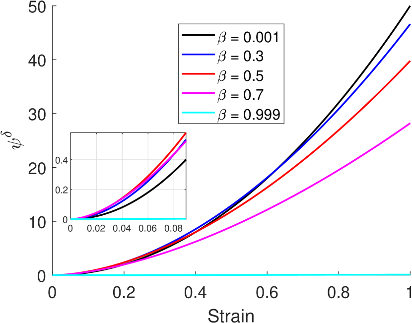
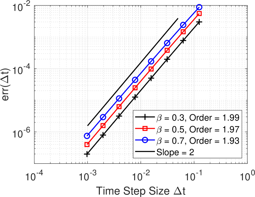
Figure 3: Numerical results for the free-energy computation with a quadratic form for $\varepsilon(t)$. (Left) $\psi^{\delta}$ vs strain with varying $\beta$. (Right) Relative error vs time-step size for varying $\beta$, with second-order accuracy.

Figure 4 presents the obtained $\mathcal{O}(N^{3})$ and $\mathcal{O}(N^{2}\log N)$ computational complexities, respectively, for the direct and FFT-based free-energy time-integration schemes. The break-even point lies at $N=200$ time-steps.

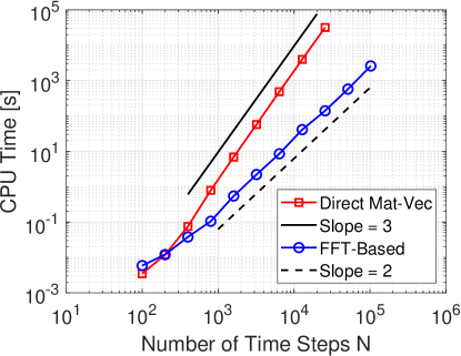
Figure 4: CPU time vs number of time-steps of the developed time-integration schemes for the fractional Helmholtz free-energy density under monotone strains.

• Cyclic Strains. We utilize a fabricated sinusoidal strain solution $\varepsilon(t)=\varepsilon_{0}\sin(\omega t)$, with $t\in(0,\,T]$, with amplitude $\epsilon_{0}$ and frequency $\omega$. The corresponding analytical solution for $\psi^{*}$ is cumbersome, and therefore not shown here. We set $\varepsilon_{0}=1$, $\omega=\pi\,[s^{-1}]$, $T=50\,[s]$, $\beta=0.5$ and $\mathbb{E}=1\,[Pa.s^{0.5}]$, and start with a sufficient number of time-steps to capture the oscillation modes. Figure 5 illustrates the obtained results, where we capture the highly oscillatory behavior for both transient and steady-state parts with second-order accuracy.

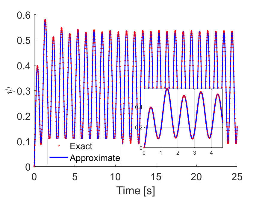
(a) Free-energy vs time.

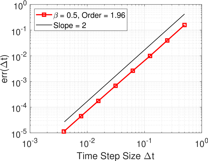
(b) Relative error vs time-step size.

Figure 5: (A) Free-energy density computations for cyclic strains vs time, $N=3200$ time-steps and $\beta=0.5$. (B) Convergence analysis showing second-order accuracy.

Example 5.2 (Fractional Visco-Elasto-Plastic Model with Damage).

We test our developed model and fractional return-mapping algorithm subject to prescribed monotone/cyclic strains. The convergence analysis is done with a benchmark solution and we analyze the quality of the anomalous damage response with respect to the fractional orders $\beta_{E},\beta_{K}$ from visco-elasticity/plasticity under different strain amplitudes/frequencies.

•  Monotone Strains. Let $\varepsilon(t)=\dot{\varepsilon}t$, where $t\in(0,\,T]$, final time $T=0.03125\,[s]$ and strain rate $\dot{\varepsilon}=0.64\,[s^{-1}]$, and therefore $\varepsilon(T)=0.02$. We set $\beta_{E}=0.5$, $\mathbb{E}=50\,[Pa.s^{0.5}]$, $\mathbb{K}=10\,[Pa.s^{\beta_{K}}]$, $\tau^{Y}=1\,[Pa]$, $S=10^{-4}\,[Pa]$ and $s=1$. A benchmark solution for the stress (see Fig.6) is computed with time-step size $\Delta t=2^{-20}\,[s]$ and varying fractional orders $\beta_{K}$, where we observe that higher values for $\beta_{K}$ led to increased hardening and damage for the prescribed strain rate.

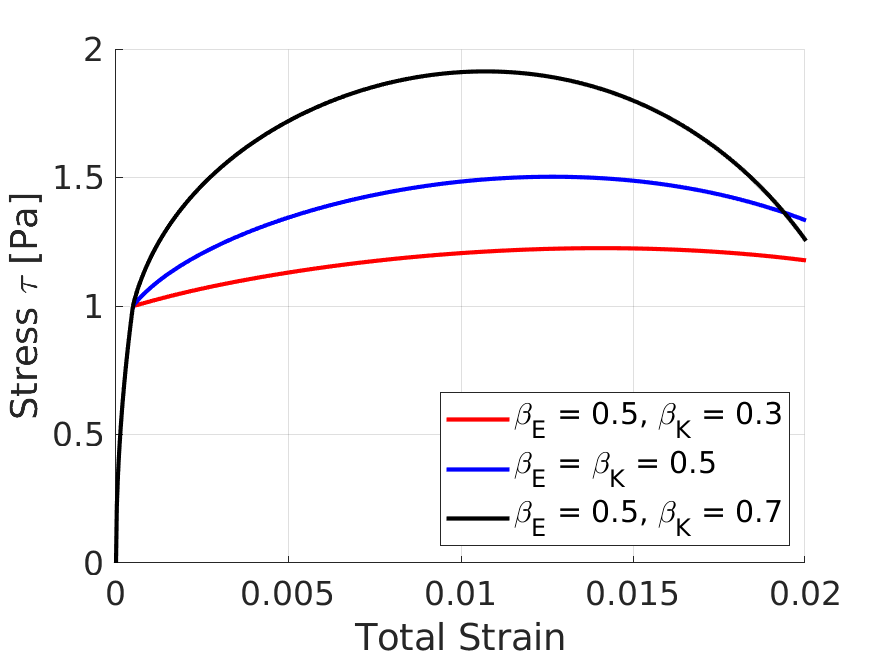
Figure 6: Stress vs strain for the benchmark solution with time-step size $\Delta t=2^{-20}$, $\beta_{E}=0.5$ and different $\beta_{K}$ values.

We observe a linear convergence rate in Figure 7(a), due to the employed backward-Euler discretization in the fractional return-mapping algorithm. A second-order computational complexity for the fractional return-mapping algorithm is also verified in Figure 7(b).

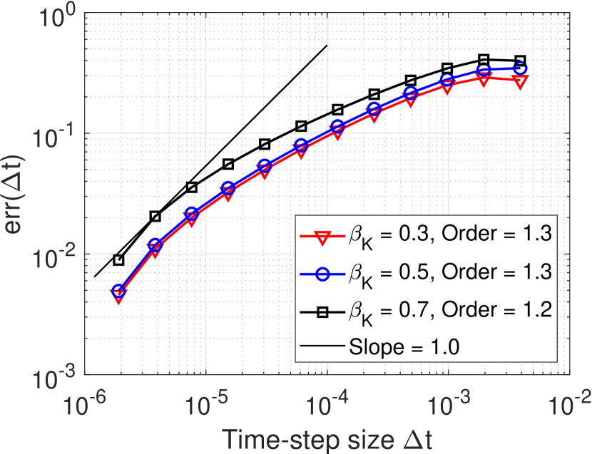
(a) Convergence behavior.

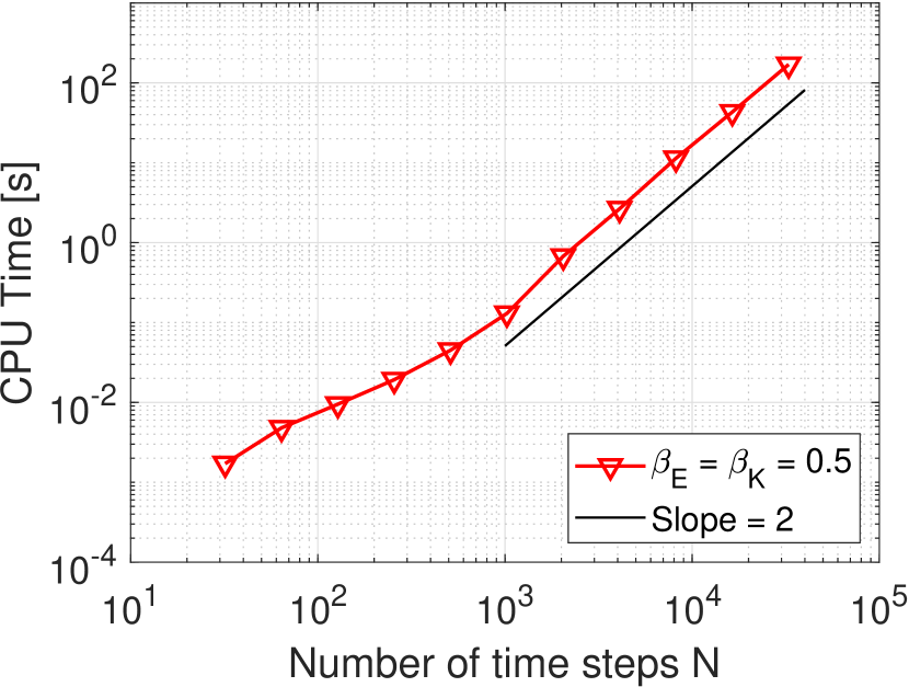
(b) Computational complexity.

Figure 7: Fractional visco-elasto-plastic model with damage under monotone strains. (A) First-order convergence behavior. (B) Computational time vs number of time-steps, with second-order computational complexity.

The influence of hardening and visco-elastic damage energy release rate is shown in Figure 8. We observe that higher damage values are obtained for $\beta_{K}=0.7$, despite the higher accumulated plastic strains for lower values of $\beta_{K}$. The higher damage is instead due to higher values of damage energy release rates shown in Figure 8(b) for $\beta_{K}=0.7$. We note that similar to the stress-strain response, the visco-elastic fractional free-energy is power-law memory-dependent on the strain rates, therefore leading to the observed anomalous behavior.

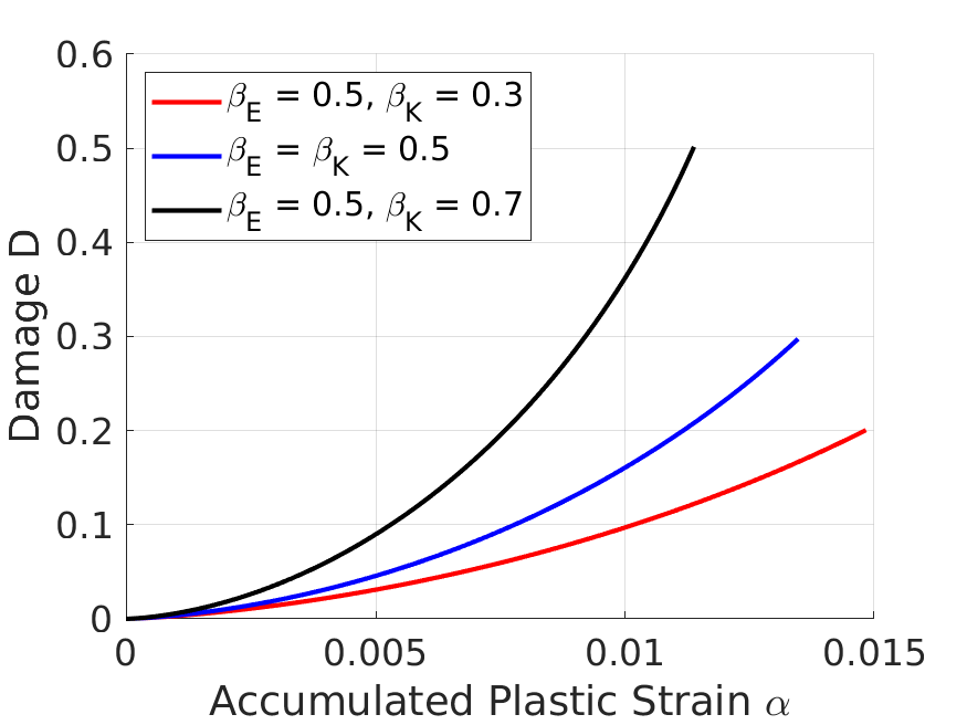
(a)

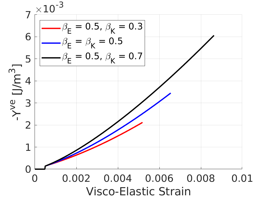
(b)

Figure 8: Developed model under monotone strains: (A) Damage vs accumulated plastic strain, with higher damage but less plasticity for higher $\beta_{K}$. (B) Damage energy release rate vs visco-elastic strains, which are both larger for higher values of fractional order $\beta_{K}$.

•  Cyclic Strains. To investigate the interplay between the damage/hardening/
viscosity and hysteresis effects, we perform a constant rate loading/unloading cyclic strain test, mathematically expressed as:

$$\varepsilon(t)=\frac{2\varepsilon_{A}}{\pi}\arcsin\left(\sin\left(2\pi\omega t\right)\right),$$

where $\varepsilon_{A}$ and $\omega$ represent, respectively, the amplitude and frequency of total strains. Here, we focus on low-cycle fatigue behavior, and therefore we set $\varepsilon=0.1$, and three strain frequencies $\omega=\{2\pi,\,4\pi,\,8\pi\}\,[s^{-1}]$, which correspond, respectively, to approximate absolute strain rates of $|\dot{\varepsilon}|\approx\{2.51,\,5.02,\,10.05\}$. We set a total time $T=10\,[s]$, and for each frequency, we use $N=\{8\,000,\,16\,000,\,32\,000\}$ time-steps, corresponding to $\Delta t=\{1.25\times 10^{-3},\,6.25\times 10^{-4},\,3.125\times 10^{-4}\}\,[s]$. The material parameters are set to $\mathbb{E}=25\,[Pa.s^{\beta_{E}}]$, $\mathbb{K}=10\,[Pa.s^{\beta_{K}}]$, $\tau^{Y}=1\,[Pa]$, $S=1\,[Pa]$ and $s=1$, where we set the fractional order values $\beta_{E}=\beta_{K}=\{0.3,\,0.5,\,0.7\}$.

The stress-strain hysteresis results are presented in Figure 9. We observe that higher frequencies led to more softening in the model, while higher values of fractional orders $\beta_{E}$, $\beta_{K}$ led to increased hardening, followed by softening.

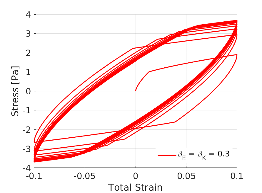
(a) $\beta_{E}=\beta_{K}=0.3$.

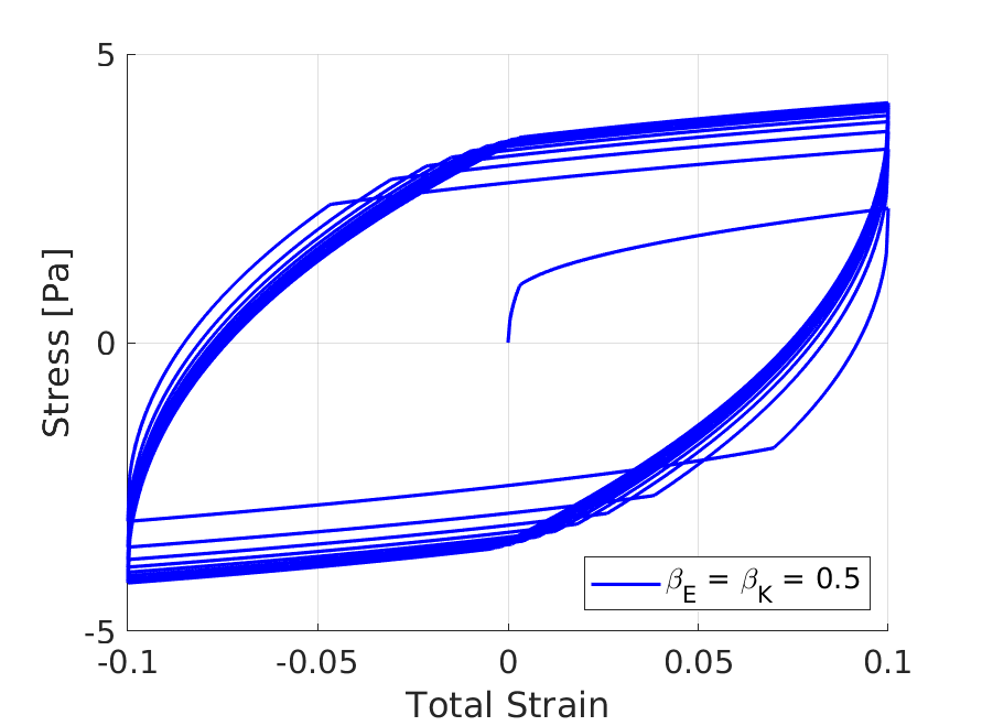
(b) $\beta_{E}=\beta_{K}=0.5$.

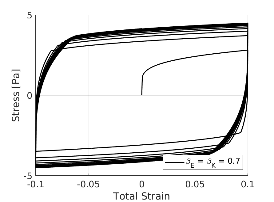
(c) $\beta_{E}=\beta_{K}=0.7$.

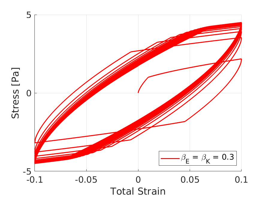
(d) $\beta_{E}=\beta_{K}=0.3$.

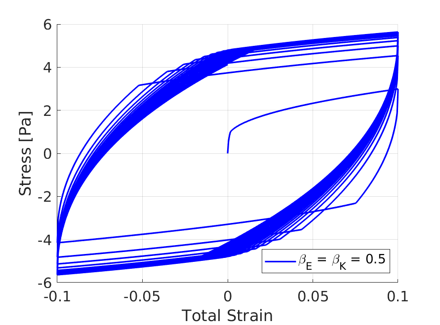
(e) $\beta_{E}=\beta_{K}=0.5$.

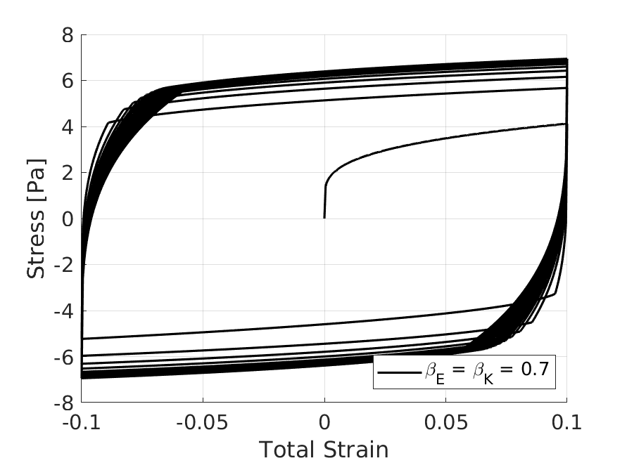
(f) $\beta_{E}=\beta_{K}=0.7$.

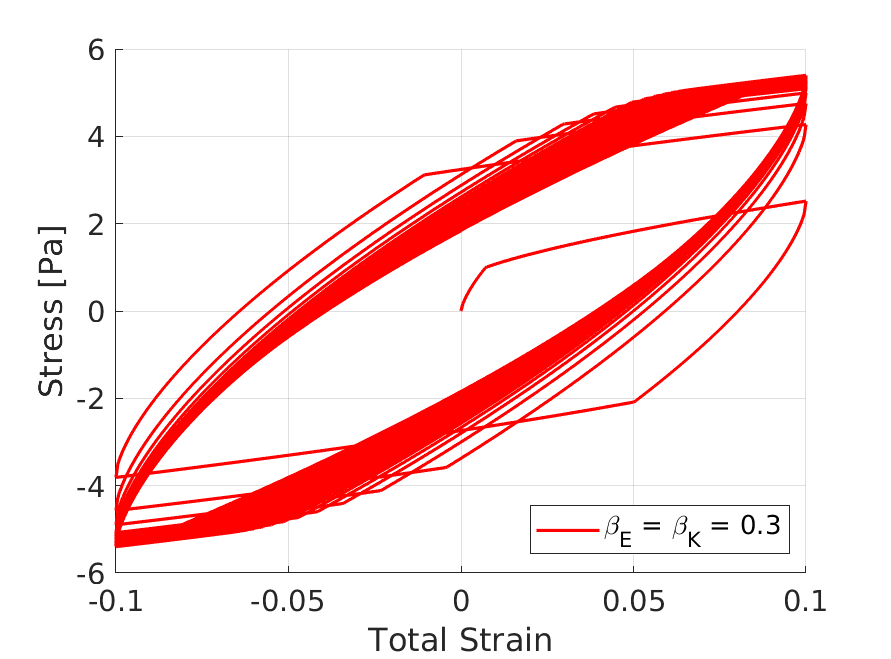
(g) $\beta_{E}=\beta_{K}=0.3$.

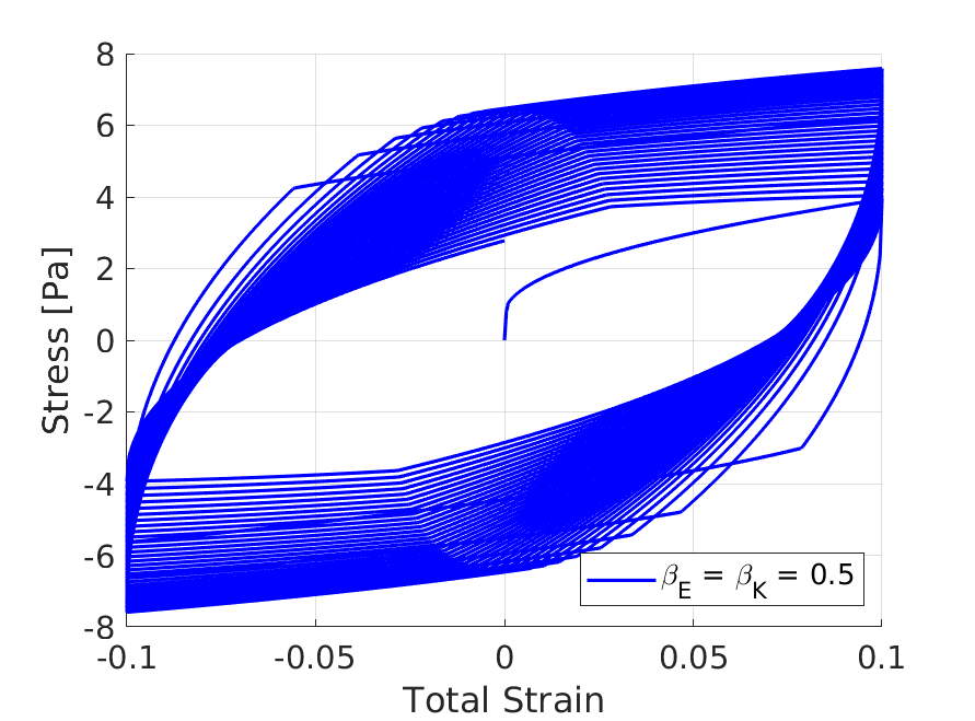
(h) $\beta_{E}=\beta_{K}=0.5$.

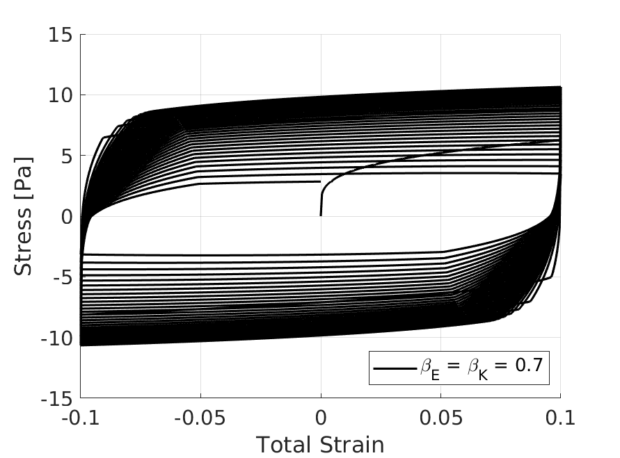
(i) $\beta_{E}=\beta_{K}=0.7$.

Figure 9: Stress hysteresis response for cyclic strains with frequencies (A)-(C) $\omega=2\pi$, (D)-(F) $\omega=4\pi$, (G)-(I) $\omega=8\pi$.

Such damage increase is illustrated in Fig. 10, where we observe that higher $\beta_{E}$ and $\beta_{K}$ values led to increased plasticity for all cases, with a significant increase of damage rates for $\beta_{E}=\beta_{K}=0.5,0.7$ when $\omega=8\pi$. We also observe from Fig. 11 that due to the anomalous nature of the fractional visco-elastic free-energy potential, the damage energy release rates substantially increase with higher fractional orders and loading rates, which contribute to the observed higher values of damage. Therefore, for this model, higher material viscosity in both visco-elastic and visco-plastic parts might be sufficient to yield lower values of damage at low frequencies due to internal dissipation mechanisms, but at higher frequencies and therefore more loading cycles, they lead to earlier material failure.

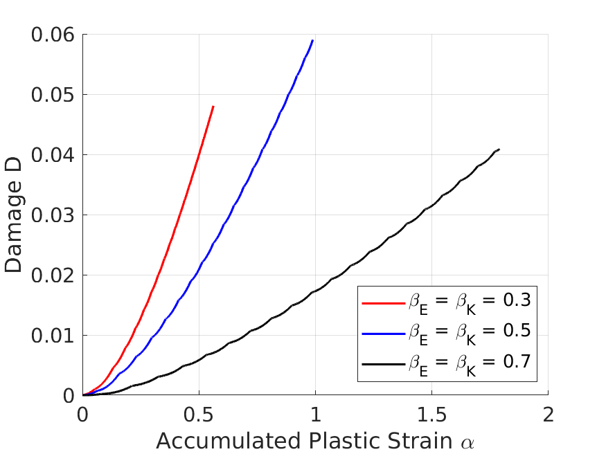
(a) $\omega=2\pi$.

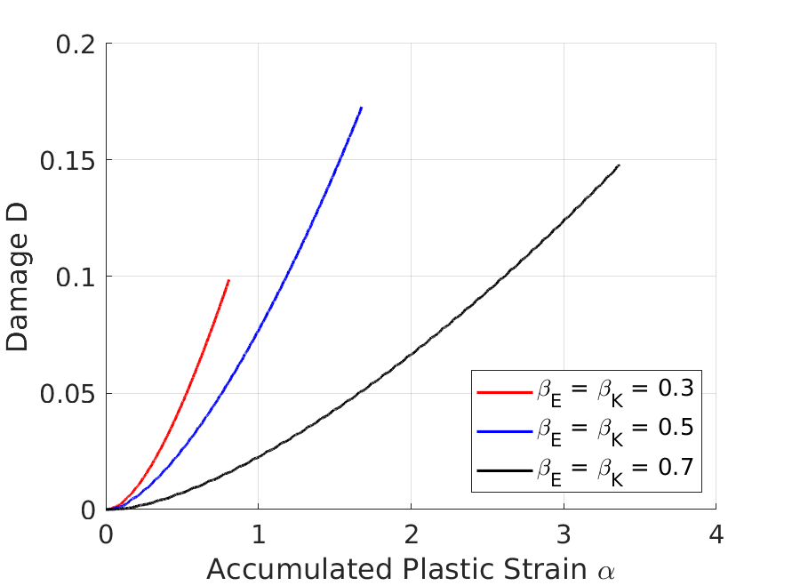
(b) $\omega=4\pi$.

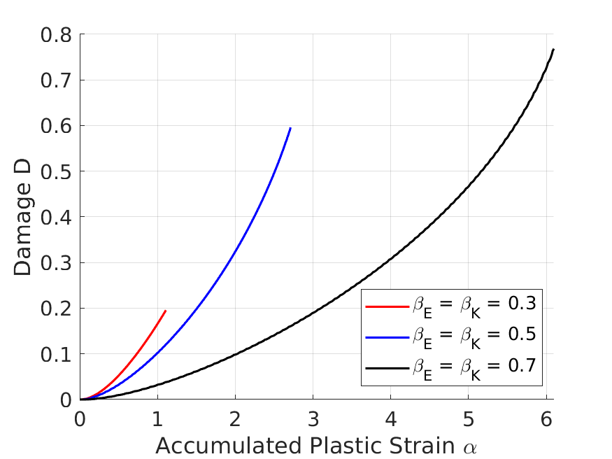
(c) $\omega=8\pi$.

Figure 10: Damage vs accumulated plastic strains with varying strain frequencies.

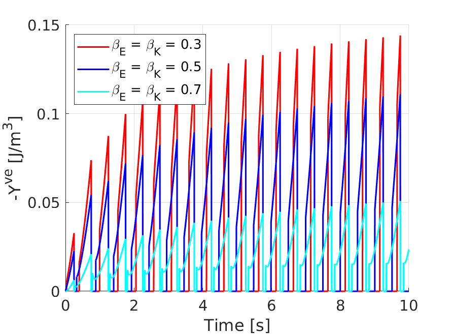
(a) $\omega=2\pi$.

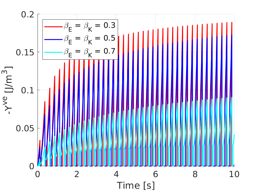
(b) $\omega=4\pi$.

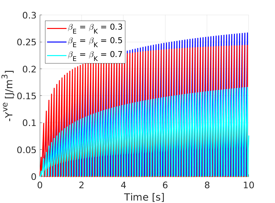
(c) $\omega=8\pi$.

Figure 11: Damage energy release rate vs time for the total strain with varying frequency.

6 Conclusions

We developed a thermodynamically consistent, fractional visco-elasto-plastic model with memory-dependent damage using fractional Helmholtz free-energies, visco-plastic/damage potentials and the Clausius-Duhem inequality. The damage energy release rate was derived from the visco-elastic free-energy to obtain a consistent bulk energy loss for anomalous materials.

A first-order, semi-implicit fractional return-mapping algorithm, which generalizes existing standard ones, was developed to solve the resulting nonlinear system of FDEs. We note that most existing algorithms for standard plasticity models are not more accurate than ours. We also developed a new FD scheme with accuracy $\mathcal{O}(\Delta t^{2-\beta})$ for the free-energy/damage energy release, with computational complexity of $\mathcal{O}(N^{2}\log N)$ through FFTs.

We also performed a set of numerical tests and observed that:

• The fractional orders $\beta_{E}$ and $\beta_{K}$ tune the competition between the plastic slip and damage energy release rate for damage evolution.

• Higher values of $\beta_{E}$, $\beta_{K}$ yielded lower damage levels for lower strain rates and cycles; However, the damage increased significantly faster than lower values of $\beta_{E},\beta_{k}$ for higher strain rates/cycles.

• For the free-energy discretization, the break-even point between the original and fast schemes was low, about $N=200$ time-steps.

• The developed discretization recovered the limit Hookean $\beta\to 0$ and Newtonian $\beta\to 1$ cases for the free-energy.

In the presence of single- to multi- singularities, the accuracy of the developed scheme can improve through a variant of a self-singularity-capturing approach [53] for all fractional operators. Nevertheless, non-smooth loading/unloading conditions pose additional challenges to develop high-order schemes for the model. In terms of efficiency, the computational bottleneck lies in the free-energy discretization, which needs further improvements before employing fast schemes for the fractional derivatives, e.g., fast convolution [61, 35] and fast multi-pole approaches [57]. Variants of the developed model can be incorporated in a straightforward fashion. The visco-elastic part could be composed of any data/design-driven arrangement of SB elements, e.g. Kelvin-Voigt, Maxwell, Kelvin-Zener [46], while adding the corresponding energy release rates to the damage potential. In addition, similar frameworks involving fractional damage energy release rates can be employed to phase field models [6]. Potential applications of the developed work could be, e.g., failure of polymers, bio-tissues, and ductile metals, where the fractional-orders $\beta_{E}$, $\beta_{K}$ can be related to the evolving fractal-like microstructure [36]. The presented model could also be employed in the context of nonlinear dynamics of mechanical systems [52, 56].

Finally, the employment of nonlocal truncated time derivatives [19] and potentials could have additional impacts on reducing the computational complexity of the developed scheme, due to the shorter memory. Furthermore, the use of such operators seems particularly interesting to naturally address the “memory reset" for internal variables such as the hardening $\alpha$ for hysteresis loading [54].

Appendix A Proof of Lemma 3.1

We take the time derivative of the free-energy (10) and obtain:

(63) $$\dot{\psi}=\int^{\infty}_{0}\tilde{E}(z)\int^{t}_{0}\exp\left(-\frac{t-s}{z}\right)\dot{\varepsilon}(s)ds\left(\frac{d}{dt}\int^{t}_{0}\exp\left(-\frac{t-s}{z}\right)\dot{\varepsilon}(s)ds\right)dz$$

with

(64) $$\frac{d}{dt}\int^{t}_{0}\exp\left(-\frac{t-s}{z}\right)\dot{\varepsilon}(s)ds=\dot{\varepsilon}(t)-\int^{t}_{0}\frac{1}{z}\exp\left(-\frac{t-s}{z}\right)\dot{\varepsilon}(s)ds.$$

Substituting (64) into (63), we obtain:

$$\dot{\psi}= \left[\int^{\infty}_{0}\tilde{E}(z)\left(\int^{t}_{0}\exp\left(-\frac{t-s}{z}\right)\dot{\varepsilon}(s)ds\right)dz\right]\dot{\varepsilon}$$

(65) $$\qquad-\int^{\infty}_{0}\frac{\tilde{E}(z)}{z}\left(\int^{t}_{0}\exp\left(-\frac{t-s}{z}\right)\dot{\varepsilon}(s)ds\right)^{2}dz.$$

Let $\mathbb{E}^{*}=\frac{\mathbb{E}}{\Gamma(1-\beta)\Gamma(\beta)}$. Note that the term inside brackets in (65) equals:

$$\int^{\infty}_{0}\tilde{E}(z)\left(\int^{t}_{0}\exp\left(-\frac{t-s}{z}\right)\dot{\varepsilon}(s)\,ds\right)\,dz$$

$$=\int^{\infty}_{0}\frac{\mathbb{E}^{*}}{z^{\beta+1}}\left(\int^{t}_{0}\exp\left(-\frac{t-s}{z}\right)\dot{\varepsilon}(s)\,ds\right)\,dz$$

$$=\mathbb{E}^{*}\int^{t}_{0}\left[\int^{\infty}_{0}z^{-(\beta+1)}\exp\left(-\frac{t-s}{z}\right)\,dz\right]\,\dot{\varepsilon}(s)\,ds$$

$$=\mathbb{E}^{*}\int^{t}_{0}\left[\int^{\infty}_{0}\frac{u^{\nu-1}}{(t-s)^{\beta}}\exp(-u)\,du\right]\,\dot{\varepsilon}(s)\,ds$$

$$=\mathbb{E}^{*}\int^{t}_{0}\left[\frac{\Gamma(\beta)}{(t-s)^{\beta}}\right]\,\dot{\varepsilon}(s)\,ds=\frac{\mathbb{E}}{\Gamma(1-\beta)}\int^{t}_{0}\frac{\dot{\varepsilon}(s)}{(t-s)^{\beta}}\,ds$$

(66) $$=\mathbb{E}\,{}^{C}_{0}\mathcal{D}^{\beta}_{t}\left(\varepsilon\right).$$

Substituting (66) into (65), and the result into (9), we obtain:

(67) $$\left[\tau-\mathbb{E}\,{}^{C}_{0}\mathcal{D}^{\beta}_{t}\left(\varepsilon\right)\right]\dot{\varepsilon}+\int^{\infty}_{0}\frac{\tilde{E}(z)}{z}\left(\int^{t}_{0}\exp\left(-\frac{t-s}{z}\right)\dot{\varepsilon}(s)ds\right)^{2}dz\geq 0.$$

Since the strain rate $\dot{\varepsilon}$ is arbitrary, we set the argument inside brackets to zero without violating the above inequality, to obtain the stress-strain relationship for the SB model:

$$\tau=\mathbb{E}\,{}^{C}_{0}\mathcal{D}^{\beta}_{t}\left(\varepsilon\right).$$

Furthermore, the remainder of (67) represents an internal positive mechanical dissipation, given by:

$$\mathcal{D}_{mech}(\varepsilon)=\int^{\infty}_{0}\frac{\tilde{E}(z)}{z}\left(\int^{t}_{0}\exp\left(-\frac{t-s}{z}\right)\dot{\varepsilon}(s)ds\right)^{2}dz\geq 0,$$

where the above inequality holds, since $z$ and $\tilde{E}(z)$ are positive.

Appendix B Proof of Theorem 4.5

We recall the mechanical dissipation (26):

(68) $$\tau\dot{\varepsilon}^{vp}-R\dot{\alpha}-Y\dot{D}+(1-D)\left(\mathcal{D}^{ve}_{mech}+\mathcal{D}^{vp}_{mech}\right)\geq 0,$$

where we must prove that the above inequality holds. Substituting (31), (32) into (26) yields:

$$\tau\mathrm{sign}(\tau)\dot{\gamma}-R\dot{\gamma}-Y\dot{D}+(1-D)\left(\mathcal{D}^{ve}_{mech}+\mathcal{D}^{vp}_{mech}\right)\geq 0,$$

Rearranging the above equation, we obtain:

$$\left[\lvert\tau\rvert-\left((1-D)\tau^{Y}+R\right)\right]\dot{\gamma}-Y\dot{D}+(1-D)\left(\tau^{Y}\dot{\gamma}+\mathcal{D}^{ve}_{mech}+\mathcal{D}^{vp}_{mech}\right)\geq 0,$$

where the first term is is related to the persistency condition [49]:

$$\left[\lvert\tau\rvert-\left((1-D)\tau^{Y}+R\left(\alpha\right)\right)\right]\dot{\gamma}=f(\tau,\alpha,D)\dot{\gamma}=0,$$

and therefore,

(69) $$\left(1-D\right)\left(\tau^{Y}\dot{\gamma}+\mathcal{D}^{ve}_{mech}+\mathcal{D}^{vp}_{mech}\right)-Y\dot{D}\geq 0.$$

We check the positiveness for each term of the above inequality. For the first term, since the damage is always positive, so is $(1-D)$. Also, we have $\tau^{Y}>0$ and $\dot{\gamma}\geq 0$ [49]. From Lemma 3.1 the mechanical dissipations $\mathcal{D}^{ve}_{mech}$ and $\mathcal{D}^{vp}_{mech}$ are also positive. For the second term, $-Y$ is positive and so is $\dot{D}$, since $D$ is a monotonically increasing function. Therefore, inequality (69) holds, and thus the developed model is thermodynamic admissible.

Appendix C Convexity of the Yield Function

Proof C.1.

Recalling (4.1.3), we have

$$f\left(\tau,\alpha,D\right) :=\lvert\tau\rvert-\left[(1-D)\tau^{Y}+R\right],$$

where $R(\alpha,D)=\left(1-D\right)\left[\mathbb{K}\,{}^{C}_{0}\mathcal{D}^{\beta_{K}}_{t}\left(\alpha\right)+H\alpha\right]$. We fix $D$ since we are interested in showing the convexity of $f$ with respect to $\tau$ and $R$. Let $x_{1}=\left(\tau_{1},R_{1}\right)$, $x_{2}=\left(\tau_{2},R_{2}\right)$, $\xi\in[0,1]$, with $R_{i}=(\alpha_{i},D)=\mathbb{K}\,{}^{C}_{0}\mathcal{D}^{\beta_{K}}_{t}\left(\alpha\right)\big{|}_{\alpha=\alpha_{i}}+H\alpha_{i}$. Therefore, we have:

$$f\left(\xi x_{1}+(1-\xi)x_{2}\right)= |\xi\tau_{1}+(1-\xi)\tau_{2}|-(1-D)\tau^{Y}-\xi R_{1}-(1-\xi)R_{2},$$

$$= |\xi\tau_{1}+(1-\xi)\tau_{2}|-\xi\left[(1-D)\tau_{Y}+R_{1}\right]$$

$$-(1-\xi)\left[(1-D)\tau^{Y}+R_{2}\right],$$

$$\leq \xi\left\{|\tau_{1}|-\left[(1-D)\tau^{Y}+R_{1}\right]\right\}\textrm{(by Jensen inequality)}$$

$$+(1-\xi)\left\{|\tau_{2}|-\left[(1-D)\tau^{Y}+R_{2}\right]\right\},$$

$$= \xi f(x_{1})+(1-\xi)f(x_{2}).$$

Appendix D Local Truncation Error for the Free-Energy Discretization

We prove the local truncation error (47) for the discretized Helmholtz free-energy density. Before we prove it, we need the following result.

Lemma D.1.

Let $\beta\in(0,1)$, then

(70) $$\int_{t_{i}}^{t_{i+1}}\left[(t_{n+1}-s)^{-\beta}-(2t_{n+1}-s)^{-\beta}\right]ds\leq C_{1}\Delta t^{1-\beta},~{}~{}~{}0\leq i\leq n,$$

where $C_{1}$ is a constant independent of $\Delta t$.

Proof D.2.

We can obtain

$$\int_{t_{i}}^{t_{i+1}}\left[(t_{n+1}-s)^{-\beta}-(2t_{n+1}-s)^{-\beta}\right]ds$$

$$= -\frac{(t_{n+1}-s)^{1-\beta}}{1-\beta}\Bigg{|}_{t_{i}}^{t_{i+1}}+\frac{(2t_{n+1}-s)^{1-\beta}}{1-\beta}\Bigg{|}_{t_{i}}^{t_{i+1}}$$

$$= \frac{\Delta t^{1-\beta}}{1-\beta}\left[(n+1-i)^{1-\beta}-(n-i)^{1-\beta}+(2n+1-i)^{1-\beta}-(2n+2-i)^{1-\beta}\right].$$

Since

$$(n+1)^{1-\beta}-n^{1-\beta}=(1-\beta)\int_{-1}^{0}(n-s)^{-\beta}ds\leq(1-\beta)n^{-\beta},~{}~{}~{}n\geq 1,$$

then, when $0\leq i\leq n-1$, we have

$$\int_{t_{i}}^{t_{i+1}}\left[(t_{n+1}-s)^{-\beta}-(2t_{n+1}-s)^{-\beta}\right]ds \leq\Delta t^{1-\beta}\left[\frac{1}{(n-i)^{\beta}}-\frac{1}{(2n+1-i)^{\beta}}\right]$$

$$\leq\frac{\Delta t^{1-\beta}}{(n-i)^{\beta}},$$

for $i=n$, it holds that

$$\int_{t_{n}}^{t_{n+1}}\left[(t_{n+1}-s)^{-\beta}-(2t_{n+1}-s)^{-\beta}\right]ds =\frac{\Delta t^{1-\beta}}{1-\beta}\left[1+(n+1)^{1-\beta}-(n+2)^{1-\beta}\right]$$

$$\leq\frac{\Delta t^{1-\beta}}{1-\beta}\left[1-\frac{1-\beta}{(n+1)^{\beta}}\right]\leq\frac{\Delta t^{1-\beta}}{1-\beta}.$$

Therefore this lemma is proved. Next, we prove the local truncation error for the free-energy discretization. From

$$\rho\psi(\varepsilon_{n+1})= \tilde{\mathbb{E}}\int_{0}^{t_{n+1}}\int_{0}^{t_{n+1}}\frac{\dot{\varepsilon}(s_{1})\dot{\varepsilon}(s_{2})}{(2t_{n+1}-s_{1}-s_{2})^{\beta}}ds_{1}ds_{2}$$

$$= \tilde{\mathbb{E}}\sum_{i,j=0}^{n}\int_{t_{i}}^{t_{i+1}}\int_{t_{j}}^{t_{j+1}}\frac{\Delta\varepsilon_{i+1}\Delta\varepsilon_{j+1}}{\Delta t^{2}(2t_{n+1}-s_{1}-s_{2})^{\beta}}ds_{1}ds_{2}+\tilde{r}_{\Delta t}^{n+1},$$

with $\tilde{\mathbb{E}}=\frac{\mathbb{E}}{2\Gamma(1-\beta)}$ and $\Delta\varepsilon_{k+1}=\varepsilon_{k+1}-\varepsilon_{k}$. We know that

$$\left|\tilde{r}_{\Delta t}^{n+1}\right|= \Bigg{|}\tilde{\mathbb{E}}\sum_{i,j=0}^{n}\int_{t_{i}}^{t_{i+1}}\int_{t_{j}}^{t_{j+1}}(2t_{n+1}-s_{1}-s_{2})^{-\beta}\left[\dot{\varepsilon}(s_{1})\dot{\varepsilon}(s_{2})-\frac{\Delta\varepsilon_{i+1}\Delta\varepsilon_{j+1}}{\Delta t^{2}}\right]ds_{1}ds_{2}\Bigg{|}$$

$$= \Bigg{|}\tilde{\mathbb{E}}\sum_{i,j=0}^{n}\int_{t_{i}}^{t_{i+1}}\int_{t_{j}}^{t_{j+1}}(2t_{n+1}-s_{1}-s_{2})^{-\beta}\left[\dot{\varepsilon}(s_{1})\dot{\varepsilon}(s_{2})-\dot{\varepsilon}(s_{1})\frac{\Delta\varepsilon_{j+1}}{\Delta t}\right.$$

$$\left.+\dot{\varepsilon}(s_{1})\frac{\Delta\varepsilon_{j+1}}{\Delta t}-\frac{\Delta\varepsilon_{i+1}\Delta\varepsilon_{j+1}}{\Delta t^{2}}\right]ds_{1}ds_{2}\Bigg{|}$$

$$= \Bigg{|}\tilde{\mathbb{E}}\sum_{i,j=0}^{n}\int_{t_{i}}^{t_{i+1}}\int_{t_{j}}^{t_{j+1}}(2t_{n+1}-s_{1}-s_{2})^{-\beta}\left[\dot{\varepsilon}(s_{1})\left(\dot{\varepsilon}(s_{2})-\frac{\Delta\varepsilon_{j+1}}{\Delta t}\right)\right.$$

$$\left.+\frac{\Delta\varepsilon_{j+1}}{\Delta t}\left(\dot{\varepsilon}(s_{1})-\frac{\Delta\varepsilon_{i+1}}{\Delta t}\right)\right]ds_{1}ds_{2}\Bigg{|}$$

$$\leq \tilde{\mathbb{E}}\Bigg{|}\sum_{i,j=0}^{n}\int_{t_{i}}^{t_{i+1}}\int_{t_{j}}^{t_{j+1}}(2t_{n+1}-s_{1}-s_{2})^{-\beta}\dot{\varepsilon}(s_{1})\left(\dot{\varepsilon}(s_{2})-\frac{\Delta\varepsilon_{j+1}}{\Delta t}\right)ds_{1}ds_{2}\Bigg{|}$$

$$+\tilde{\mathbb{E}}\Bigg{|}\sum_{i,j=0}^{n}\frac{\Delta\varepsilon_{j+1}}{\Delta t}\int_{t_{i}}^{t_{i+1}}\int_{t_{j}}^{t_{j+1}}(2t_{n+1}-s_{1}-s_{2})^{-\beta}\left(\dot{\varepsilon}(s_{1})-\frac{\Delta\varepsilon_{i+1}}{\Delta t}\right)ds_{1}ds_{2}\Bigg{|}$$

$$:= I_{1}+I_{2},$$

where

$$I_{1}=\tilde{\mathbb{E}}\Bigg{|}\sum_{i,j=0}^{n}\int_{t_{i}}^{t_{i+1}}\int_{t_{j}}^{t_{j+1}}(2t_{n+1}-s_{1}-s_{2})^{-\beta}\dot{\varepsilon}(s_{1})\left(\dot{\varepsilon}(s_{2})-\frac{\Delta\varepsilon_{j+1}}{\Delta t}\right)ds_{1}ds_{2}\Bigg{|},$$

and

$$I_{2}=\tilde{\mathbb{E}}\Bigg{|}\sum_{i,j=0}^{n}\frac{\Delta\varepsilon_{j+1}}{\Delta t}\int_{t_{i}}^{t_{i+1}}\int_{t_{j}}^{t_{j+1}}(2t_{n+1}-s_{1}-s_{2})^{-\beta}\left(\dot{\varepsilon}(s_{1})-\frac{\Delta\varepsilon_{i+1}}{\Delta t}\right)ds_{1}ds_{2}\Bigg{|}.$$

Assume $\varepsilon(t)\in C^{2}[0,T]$, then one can obtain that:

$$\varepsilon(t)\leq C_{2},~{}~{}~{}\dot{\varepsilon}(t)\leq C_{3},~{}t\in[0,T].$$

On each small interval $[t_{i},t_{i+1}]~{}(0\leq i\leq n)$, denoting the linear interpolation function of $\varepsilon(t)$ as $\Pi_{i}\varepsilon(t)$:

$$\Pi_{i}\varepsilon(t)=\frac{t-t_{i+1}}{t_{i}-t_{i+1}}\varepsilon_{i}+\frac{t-t_{i}}{t_{i+1}-t_{i}}\varepsilon_{i+1},$$

it follows from the linear interpolation theory that

$$\varepsilon(t)-\Pi_{i}\varepsilon(t)=\frac{\varepsilon^{\prime\prime}(\xi_{i})}{2}(t-t_{i})(t-t_{i+1})\leq c_{i}\Delta t^{2},~{}~{}~{}t\in[t_{i},t_{i+1}],~{}\xi_{i}\in(t_{i},t_{i+1}),$$

with $0\leq i\leq n$, and here $c_{i}$ is a constant independent of $\Delta t$.

For $I_{1}$, we have

$$I_{1}= \tilde{\mathbb{E}}\Bigg{|}\sum_{i,j=0}^{n}\int_{t_{i}}^{t_{i+1}}\dot{\varepsilon}(s_{1})\int_{t_{j}}^{t_{j+1}}(2t_{n+1}-s_{1}-s_{2})^{-\beta}\left[\varepsilon(s_{2})-\Pi_{j}\varepsilon(s_{2})\right]^{\prime}ds_{1}ds_{2}\Bigg{|}$$

$$= \tilde{\mathbb{E}}\Bigg{|}\sum_{i,j=0}^{n}\int_{t_{i}}^{t_{i+1}}\dot{\varepsilon}(s_{1})\int_{t_{j}}^{t_{j+1}}(2t_{n+1}-s_{1}-s_{2})^{-\beta}d\left[\varepsilon(s_{2})-\Pi_{j}\varepsilon(s_{2})\right]ds_{1}\Bigg{|}$$

$$= \beta\tilde{\mathbb{E}}\Bigg{|}\sum_{i,j=0}^{n}\int_{t_{i}}^{t_{i+1}}\dot{\varepsilon}(s_{1})\int_{t_{j}}^{t_{j+1}}\left[\varepsilon(s_{2})-\Pi_{j}\varepsilon(s_{2})\right](2t_{n+1}-s_{1}-s_{2})^{-\beta-1}ds_{1}ds_{2}\Bigg{|}$$

$$\leq \beta\tilde{\mathbb{E}}\Bigg{|}\sum_{i,j=0}^{n}\int_{t_{i}}^{t_{i+1}}\dot{\varepsilon}(s_{1})\int_{t_{j}}^{t_{j+1}}c_{j}\Delta t^{2}(2t_{n+1}-s_{1}-s_{2})^{-\beta-1}ds_{1}ds_{2}\Bigg{|}$$

$$\leq \beta\tilde{\mathbb{E}}C_{4}\Delta t^{2}\Bigg{|}\sum_{i=0}^{n}\int_{t_{i}}^{t_{i+1}}\dot{\varepsilon}(s_{1})\int_{0}^{t_{n+1}}(2t_{n+1}-s_{1}-s_{2})^{-\beta-1}ds_{1}ds_{2}\Bigg{|}$$

$$= \tilde{\mathbb{E}}C_{4}\Delta t^{2}\Bigg{|}\sum_{i=0}^{n}\int_{t_{i}}^{t_{i+1}}\dot{\varepsilon}(s_{1})\left[(t_{n+1}-s_{1})^{-\beta}-(2t_{n+1}-s_{1})^{-\beta}\right]ds_{1}\Bigg{|}$$

$$\leq \tilde{\mathbb{E}}C_{3}C_{4}\Delta t^{2}\Bigg{|}\sum_{i=0}^{n}\int_{t_{i}}^{t_{i+1}}\left[(t_{n+1}-s_{1})^{-\beta}-(2t_{n+1}-s_{1})^{-\beta}\right]ds_{1}\Bigg{|},$$

where $C_{4}=\max\limits_{0\leq j\leq n}c_{j}$. For $I_{2}$, it holds that

$$I_{2}= \tilde{\mathbb{E}}\Bigg{|}\sum_{i,j=0}^{n}\frac{\Delta\varepsilon_{j+1}}{\Delta t}\int_{t_{i}}^{t_{i+1}}\int_{t_{j}}^{t_{j+1}}(2t_{n+1}-s_{1}-s_{2})^{-\beta}\left[\varepsilon(s_{1})-\Pi_{i}\varepsilon(s_{1})\right]^{\prime}ds_{1}ds_{2}\Bigg{|}$$

$$= \tilde{\mathbb{E}}\Bigg{|}\sum_{i,j=0}^{n}\frac{\Delta\varepsilon_{j+1}}{\Delta t}\int_{t_{j}}^{t_{j+1}}\int_{t_{i}}^{t_{i+1}}(2t_{n+1}-s_{1}-s_{2})^{-\beta}d\left[\varepsilon(s_{1})-\Pi_{i}\varepsilon(s_{1})\right]ds_{2}\Bigg{|}$$

$$= \beta\tilde{\mathbb{E}}\Bigg{|}\sum_{i,j=0}^{n}\frac{\Delta\varepsilon_{j+1}}{\Delta t}\int_{t_{j}}^{t_{j+1}}\int_{t_{i}}^{t_{i+1}}\left[\varepsilon(s_{1})-\Pi_{i}\varepsilon(s_{1})\right](2t_{n+1}-s_{1}-s_{2})^{-\beta-1}ds_{1}ds_{2}\Bigg{|}$$

$$\leq \beta\tilde{\mathbb{E}}\Bigg{|}\sum_{i,j=0}^{n}\frac{\Delta\varepsilon_{j+1}}{\Delta t}\int_{t_{j}}^{t_{j+1}}\int_{t_{i}}^{t_{i+1}}c_{i}\Delta t^{2}(2t_{n+1}-s_{1}-s_{2})^{-\beta-1}ds_{1}ds_{2}\Bigg{|}$$

$$\leq \beta\tilde{\mathbb{E}}C_{5}\Delta t\Bigg{|}\sum_{j=0}^{n}\Delta\varepsilon_{j+1}\int_{t_{j}}^{t_{j+1}}\int_{0}^{t_{n+1}}(2t_{n+1}-s_{1}-s_{2})^{-\beta-1}ds_{1}ds_{2}\Bigg{|}$$

$$= \tilde{\mathbb{E}}C_{5}\Delta t\Bigg{|}\sum_{j=0}^{n}\Delta\varepsilon_{j+1}\int_{t_{j}}^{t_{j+1}}\left[(t_{n+1}-s_{2})^{-\beta}-(2t_{n+1}-s_{2})^{-\beta}\right]ds_{2}\Bigg{|},$$

where $C_{5}=\max\limits_{0\leq i\leq n}c_{i}$. Then, it follows from Lemma D.1 that

$$I_{1}+I_{2}\leq \frac{n\mathbb{E}C_{1}C_{3}C_{4}\Delta t^{3-\beta}}{2\Gamma(1-\beta)}+\frac{\mathbb{E}C_{1}C_{5}\Delta t^{2-\beta}}{2\Gamma(1-\beta)}\Bigg{|}\sum_{j=0}^{n}\Delta\varepsilon_{j+1}\Bigg{|}$$

$$= \frac{\mathbb{E}C_{1}C_{3}C_{4}T\Delta t^{2-\beta}}{2\Gamma(1-\beta)}+\frac{\mathbb{E}C_{1}C_{5}\Delta t^{2-\beta}}{2\Gamma(1-\beta)}\big{|}\varepsilon_{n+1}-\varepsilon_{0}\big{|}$$

$$\leq \frac{\mathbb{E}C_{1}(C_{3}C_{4}T+2C_{2}C_{5})}{2\Gamma(1-\beta)}\Delta t^{2-\beta}.$$

References

• [1] K. Adolfsson, M. Enelund, and P. Olsson, On the fractional order model of viscoelasticity, Mech. Time-Depend. Mat., 9 (2005), pp. 15–34.
• [2] G. Alfano and M. Musto, Thermodynamic derivation and damage evolution for a fractional cohesive zone model, J. Eng. Mech., 143 (2017).
• [3] A. Bejan, Advanced Engineering Thermodynamics, Fourth Edition, Wiley, 2016.
• [4] G. Blair, B. Veinoglou, and B. Caffyn, Limitations of the Newtonian time scale in relation to non-equilibrium rheological states and a theory of quasi-properties, Proc. R. Soc. Lond. A, 189 (1947), pp. 69–87.
• [5] S. Blair and F. Coppen, The estimation of firmness in soft materials, Amer. J. Psychol., 56 (1943), pp. 234–246.
• [6] J. Boldrini, E. B. de Moraes, L. Chiarelli, F. Fumes, and M. Bittencourt, A non-isothermal thermodynamically consistent phase field framework for structural damage and fatigue, Comput. Methods Appl. Mech. Eng., 312 (2016), pp. 395–427.
• [7] N. Bonadkar, R. Gerum, M. Kuhn, M. Sporer, A. Lippert, W. Schneider, K. Aifantis, and B. Fabry, Mechanical plasticity of cells, Nat. Mater., 15 (2016), pp. 1090 – 1094.
• [8] P.-O. Bouchard, L. Bourgeon, S. Fayolle, and K. Mocellin, An enhanced lemaitre model formulation for materials processing damage computation, Int. J. Mater. Form., 4 (2011), pp. 299–315.
• [9] A. Burlon, F. Pinnola, and M. Zingales, A numerical assessment of the free energy function for fractional-order relaxation, in ICFDA‘14 - International Conference on Fractional Differentiation and its Applications, Catania, Italy, 2014.
• [10] T.-S. Cao, A. Gaillac, P. Montmitonnet, and P.-O. Bouchard, Identification methodology and comparison of phenomenological ductile damage models via hybrid numerical–experimental analysis of fracture experiments conducted on a zirconium alloy, Int. J. Solids Struct., 50 (2013), pp. 3984–3999.
• [11] W. Cao, F. Zeng, Z. Zhongqiang, and G. Karniadakis, Implicit-explicit difference schemes for nonlinear fractional differential equations with nonsmooth solutions, SIAM J. Sci. Comput., 38 (2016), pp. A3070–A3093.
• [12] M. Caputo and M. Fabrizio, Damage and fatigue described by a fractional derivative model, J. Comp. Phys., 293 (2015), pp. 400 – 408.
• [13] E. de Souza Neto, D. Perić, and D. Owen, Computational Methods for Plasticity: Theory and Applications, John Wiley & Sons, 2008.
• [14] M. D’Elia and M. Gunzburger, The fractional laplacian operator on bounded domains as a special case of the nonlocal diffusion operator, Comput. Math. Appl., 66 (2013), pp. 1245–1260.
• [15] L. Deseri, M. DiPaola, and M. Zingales, Free energy and states of fractional-order hereditariness, Int. J. Solids Struct., 51 (2014), pp. 3156 – 3167.
• [16] K. Diethelm, N. J. Ford, and A. D. Freed, Detailed error analysis for a fractional Adams method, Numer. Algorithms, 36 (2004), pp. 31–52.
• [17] D. Dolićanin-Đekić, On a new class of constitutive equations for linear viscoelastic body, Fract. Calc. Appl. Anal., 20 (2017), pp. 521–536.
• [18] Q. Du, M. Gunzburger, R. B. Lehoucq, and K. Zhou, A nonlocal vector calculus, nonlocal volume–constrained problems, and nonlocal balance laws, Math. Models Methods Appl. Sci., 23 (2013), pp. 493–540.
• [19] Q. Du, J. Yang, and Z. Zhou, Analysis of a nonlocal-in-time parabolic equation, Discrete Contin. Dyn. Sys. Ser. B, 22 (2017), pp. 339–368.
• [20] M. Fabrizio, Fractional rheological models for thermomechanical systems. dissipation and free energies, Fract. Calc. Appl. Anal., 17 (2014), pp. 206 – 223.
• [21] L. Feng and V. Linetsky, Pricing options in jump-diffusion models: An extrapolation approach, Oper. Res., 56 (2008), pp. 304–325.
• [22] O. Giraldo-Londoño, G. Paulino, and W. Buttlar, Fractional calculus derivation of a rate-dependent PPR-based cohesive fracture model: theory, implementation, and numerical results, Int. J. Fract., 216 (2019), pp. 1–29.
• [23] A. Giusti, On infinite order differential operators in fractional viscoelasticity, Fract. Calc. Appl. Anal., 20 (2017), pp. 854–867.
• [24] M. Gurtin, E. Fried, and L. Anand, The mechanics and thermodynamics of continua, Cambridge University Press, 2010.
• [25] X. Hei, W. Chen, G. Pang, R. Xiao, and C. Zhang, A new visco-elasto-plastic model via time-space derivative., Mech. Time-Depend. Mater., 22 (2018), pp. 129–141.
• [26] A. Jaishankar and G. McKinley, Power-law rheology in the bulk and at the interface: quasi-properties and fractional constitutive equations, Proc R Soc A 469: 20120284, (2013).
• [27] J. Kang, F. Zhou, C. Liu, and Y. Liu, A fractional non-linear creep model for coal considering damage effect and experimental validation, Int. J. Nonlin. Mech., 76 (2015), pp. 20–28.
• [28] E. Kharazmi and M. Zayernouri, Operator-based uncertainty quantification of stochastic fractional pdes, ASME J. Verif. Valid. Uncert. (in press), (2018).
• [29] E. Kharazmi and M. Zayernouri, Fractional sensitivity equation method: Applications to fractional model construction, J. Sci. Comput., 80 (2019), pp. 110–140.
• [30] J. Lemaitre, A course on damage mechanics, Springer, 1996.
• [31] J. Lemaitre and R. Desmorat, Engineering Damage Mechanics, Springer, 2005.
• [32] Y. Lin and C. Xu, Finite difference/spectral approximations for the time-fractional diffusion equation, J. Comp. Phys., 225 (2007), pp. 1533–1552.
• [33] A. Lion, On the thermodynamics of fractional damping elements, Continuum Mech. Thermodyn., 9 (1997), pp. 83 – 96.
• [34] C. Lubich, Discretized fractional calculus, SIAM J. Math. Anal., 17 (1986), pp. 704–719.
• [35] C. Lubich and A. Schädle., Fast convoluion for nonreflecting boundary conditions, SIAM J. Sci. Comput., 24 (2002), pp. 161–182.
• [36] S. Mashayekhi, Y. Hussaini, and W. Oates, A physical interpretation of fractional viscoelasticity based on the fractal structure of media: Theory and experimental validation, J. Mech. Phys. Solids, 128 (2019), pp. 137–150.
• [37] F. Meral, T. Royston, and R. Magin, Fractional calculus in viscoelasticity: An experimental study, Commun. Nonlinear Sci. Numer. Simul., 15 (2010), pp. 939–945.
• [38] M. Naghibolhosseini, Estimation of outer-middle ear transmission using DPOAEs and fractional-order modeling of human middle ear, PhD thesis, City University of New York, NY., 2015.
• [39] M. Naghibolhosseini and G. Long, Fractional-order modelling and simulation of human ear, Int. J. Comput. Math., 95 (2018), pp. 1257–1273.
• [40] S. Näsholm and S. Holm, On a fractional zener elastic wave equation, Fract. Calc. Appl. Anal., 16 (2013), pp. 26–60.
• [41] I. Podlubny, Fractional Differential Equations, San Diego, CA, USA: Academic Press, 1999.
• [42] E. Roux and P.-O. Bouchard, On the interest of using full field measurements in ductile damage model calibration, Int. J. Solids Struct., 72 (2015), pp. 50–62.
• [43] M. Samiee, A. Akhavan-Safaei, and M. Zayernouri, A fractional subgrid-scale model for turbulent flows: Theoretical formulation and a priori study, arXiv preprint arXiv:1909.09943, (2019).
• [44] M. Samiee, M. Zayernouri, and M. M. Meerschaert, A unified spectral method for FPDEs with two-sided derivatives; part I: A fast solver, J. Comp. Phys., 385 (2019), pp. 225–243.
• [45] M. Samiee, M. Zayernouri, and M. M. Meerschaert, A unified spectral method for FPDEs with two-sided derivatives; part II: Stability, and error analysis, J. Comp. Phys., 385 (2019), pp. 244–261.
• [46] H. Schiessel, Generalized viscoelastic models: their fractional equations with solutions, J. Phys. A: Math. Gen., 28 (1995), pp. 6567–6584.
• [47] H. Schiessel and A. Blumen, Hierarchical analogues to fractional relaxation equations, J. Phys. A: Math. Gen., 26 (1993), pp. 5057–5069.
• [48] J. Simo, On a fully three-dimensional finite-strain viscoelastic damage model: Formulation and computational aspects, Comp. Methods Appl. Mech. Eng., 60 (1987), pp. 153–173.
• [49] J. Simo and T. Hughes, Computational inelasticity, Springer, 1998.
• [50] W. Sumelka, Fractional viscoplasticity, Mech. Res. Commun., 56 (2014), pp. 31–36.
• [51] Y. Sun and W. Sumelka, Fractional viscoplastic model for soils under compression, Acta Mech., 230 (2019), pp. 3365–3377.
• [52] J. Suzuki and P. Muñoz Rojas, Transient analysis of geometrically non-linear trusses considering coupled plasticity and damage, Tenth World Congress on Computational Mechanics, 1 (2014), pp. 322–341.
• [53] J. Suzuki and M. Zayernouri, An automated singularity-capturing scheme for fractional differential equations., arXiv:1810.12219, (2018).
• [54] J. Suzuki, M. Zayernouri, M. Bittencourt, and G. Karniadakis, Fractional-order uniaxial visco-elasto-plastic models for structural analysis, Comput. Methods Appl. Mech. Eng., 308 (2016), pp. 443 – 467.
• [55] H. Tang, D. Wang, R. Huang, X. Pei, and W. Chen, A new rock creep model based on variable-order fractional derivatives and continuum damage mechanics, B. Eng. Geol. Environ., 77 (2018), pp. 375–383.
• [56] P. Varghaei, E. Kharazmi, J. Suzuki, and M. Zayernouri, Vibration analysis of geometrically nonlinear and fractional viscoelastic cantilever beams, arXiv preprint arXiv:1909.02142, (2019).
• [57] M. Vikram, A. Baczewski, B. Shanker, and L. Kempel, Accelerated cartesian expansion (ACE) based framework for the rapid evaluation of diffusion, lossy wave, and klen-gordon potentials, J. Comp. Phys., 229 (2010), pp. 9119–9134.
• [58] U. Wegst, H. Bai, E. Saiz, A. Tomsia, and R. Ritchie, Bioinspired structural materials, Nat. Mater., 14 (2015), pp. 23–36.
• [59] R. Xiao, H. Sun, and W. Chen, A finite deformation fractional viscoplastic model for the glass transition behavior of amorphous polymers, Int. J. Nonlin. Mech., 93 (2017), pp. 7–14.
• [60] M. Zayernouri and A. Matzavinos, Fractional Adams-Bashforth/Moulton methods: An application to the fractional Keller-Segel chemotaxis system., J. Comp. Phys., 317 (2016), pp. 1–14.
• [61] F. Zeng, I. Turner, and K. Burrage, A stable fast time-stepping method for fractional integral and derivative operators, J. Sci. Comput., (2018).
• [62] C. Zhang, Z. Zhu, S. Zhu, D. He, D. Zhu, J. Liu, and S. Meng, Nonlinear creep damage constitutive model of concrete based on fractional calculus theory, Materials, 12 (2014), pp. 1 – 14.
• [63] Y. Zhou, J. Suzuki, C. Zhang, and M. Zayernouri, Fast IMEX time integration of nonlinear stiff fractional differential equations, arXiv preprint arXiv:1909.04132, (2019).