Orthogonal ring patterns in the plane

Abstract.

We introduce orthogonal ring patterns consisting of pairs of concentric circles generalizing circle patterns. We show that orthogonal ring patterns are governed by the same equation as circle patterns. For every ring pattern there exists a one parameter family of patterns that interpolates between a circle pattern and its dual. We construct ring patterns analogues of the Doyle spiral, Erf and $z^{\alpha}$ functions. We also derive a variational principle and compute ring patterns based on Dirichlet and Neumann boundary conditions.

1. Introduction

The theory of circle patterns can be seen as a discrete version of conformal maps. Schramm [6] has studied orthogonal circle patterns on the ${\mathbb{Z}}^{2}$-lattice, has proven their convergence to conformal maps and constructed discrete analogs of some entire holomorphic functions. Circle patterns are described by a variational principle [5], which is given in terms of volumes of ideal hyperbolic polyhedra [4]. We introduce orthogonal ring patterns that are natural generalizations of circle patterns. Our theory of orthogonal ring patterns has its origin in discrete differential geometry of S-isothermic cmc surfaces [3]. Recently, orthogonal double circle patterns (ring patterns) on the sphere have been used to construct discrete surfaces S-cmc by Tellier et al. [7].

We start Sect. 2 with a definition of orthogonal ring patterns and their elementary properties. In particular we show that all rings have the same area. Our main Theorem 2.4 shows that ring patterns are described by an equation for variables at the vertices. Furthermore, each ring pattern comes with a natural $1$-parameter family of patterns. In Sect. 3 we show that as the area of the rings goes to zero the ring patterns converge to orthogonal circle patterns. In the following Sect. 4 we introduce ring patterns analogs of Doyle spirals, the Erf function, $z^{\alpha}$ for $\alpha\in(0,2]$, and the logarithm. Finally, we introduce a variational principle to construct ring patterns for given Dirichlet or Neumann boundary conditions. A remarkable fact that we explore is that the orthogonal ring and circle patterns in ${\mathbb{R}}^{2}$ are governed by the same integrable equation. In a subsequent publication we plan to develop a theory of ring patterns in a sphere and hyperbolic space. They are governed by equations in elliptic functions that belong to the class of discrete integrable systems classified in [1].

2. Orthogonal ring patterns

In this section, we will introduce orthogonal ring patterns and show that the existence of such the patterns is governed by the same equation as the existence of orthogonal circle patterns.

We will consider cell complex $G$ defined by a subset of the quadrilaterals of the ${\mathbb{Z}}^{2}$ lattice in ${\mathbb{R}}^{2}$. The vertices $V(G)$ of the complex $G$ are indexed by $(m,n)\in{\mathbb{Z}}^{2}$ and denoted by $v_{m,n}$. Each of its inner vertices has four neighbors, the vertices with less neighbors are called boundary vertices. The vertices of the dual cell complex $G^{*}$ are identified with the 2-cells of $G$, and the edges of $G^{*}$ correspond to the inner edges of $G$, i.e. to the edges shared by two neighboring 2-cells. We assume that $G$ and $G^{*}$ are simply connected. The oriented edges are given by pairs of vertices and are either horizontal $(v_{m,n},v_{m+1,n})$ or vertical $(v_{m,n},v_{m,n+1})$.

A ring is a pair of two concentric circles in ${\mathbb{R}}^{2}$ that form a ring (annulus). We identify the vertices with the centers and denote the inner circle and its radius by small letters $c$ and $r$, and the outer circle and its radius by capital letters $C$ and $R$. We assign an orientation to the ring by allowing $r$ to be negative: positive radius corresponds to counter-clockwise and negative radius to clockwise orientation. The outer radius will always be positive. The area of a ring is given by $(R^{2}-r^{2})\pi$. Subscripts are used to associate circles and radii to vertices of the complex, e.g., $c_{m,n}$ is the inner circle associated with the vertex $v_{m,n}$.

Definition 2.1 (Orthogonal ring patterns).

An orthogonal ring pattern consists of rings associated to the vertices of $G$ satisfying the following properties:

1. The rings associated to neighboring vertices $v_{i}$ and $v_{j}$ intersect orthogonally, i.e., the outer circle $C_{i}$ of the one vertex intersects the inner circle $c_{j}$ of the other vertex orthogonally and vice versa (see Fig. 1, left).

2. In each square of $G$ the inner circles $c_{m,n}$ and $c_{m+1,n+1}$ and the outer circles $C_{m,n+1}$ and $C_{m+1,n}$ pass through one point. (Then orthogonality implies that the two inner and the two outer circles touch in this point. see Fig. 1, center).

3. For any ring $(C_{m,n},c_{m,n})$ the four touching points $C_{m,n}\cap C_{m+1,n-1}$, $c_{m,n}\cap c_{m+1,n+1}$, $C_{m,n}\cap C_{m-1,n+1}$ and $c_{m,n}\cap c_{m-1,n-1}$ have the same orientation as $c_{m,n}$, i.e., are in counter-clockwise order if $r_{m,n}$ is positive and in clockwise order if $r_{m,n}$ is negative.

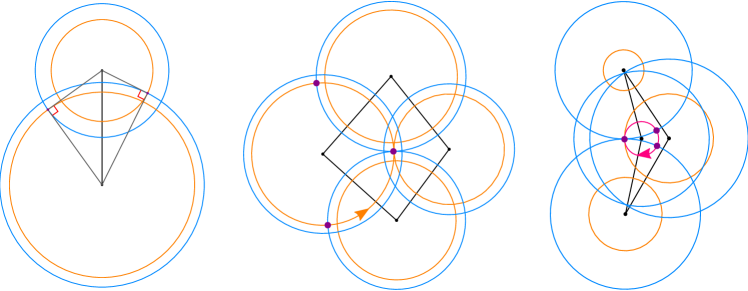
Figure 1. Left: Two orthogonally intersecting rings. Center: The inner circles touch along one diagonal of a quadrilateral and the outer circles along the other diagonal. The touching point coincides. Right: If the orientation (i.e., signed radii) of the inner circles differ, then the centers lie on the same side of the common tangent.

The orthogonal intersection of neighboring rings has the following implication for their areas.

Lemma 2.2.

Consider two rings with radii $r_{i},R_{i}$ and $r_{j},R_{j}$ that intersect orthogonally. Then the two rings have the same area.

Proof.

By Pythagoras’ Theorem the square of the distance $d$ between the circle centers is $R_{i}^{2}+r_{j}^{2}=d^{2}=r_{i}^{2}+R_{j}^{2}$ since the inner and outer circles are intersecting orthogonally. This equation is equivalent to the equality of the ring areas $(R_{i}^{2}-r_{i}^{2})\pi=(R_{j}^{2}-r_{j}^{2})\pi$. ∎

The constant area allows us to use a single variable $\rho_{i}$ to express the inner and the outer radii of the rings in the following way: Consider an orthogonal ring pattern with constant ring area $A_{0}=\pi\ell_{0}^{2}$, that is, for the radii $r_{i},R_{i}$ of all vertices $v_{i}\in V(G)$ we have $R_{i}^{2}-r_{i}^{2}=\ell_{0}^{2}$. Then for each vertex we can choose a single variable $\rho_{i}$ by setting

(1) $$R_{i}=\ell_{0}\cosh(\rho_{i})\quad\text{and}\quad r_{i}=\ell_{0}\sinh(\rho_{i})\,.$$

We will call those new variables $\rho$-radii. The orientation of the rings is encoded in the sign of the $\rho$-radii. In Sect. 3 we consider the limit of orthogonal ring patterns as the area goes to zero. The $\rho$-radii become the logarithmic radii of a Schramm type orthogonal circle pattern [6] in the limit.

As in the case of orthogonal circle patterns there exist families of vertices $V_{e}=\{(m,n)\in{\mathbb{Z}}^{2}\,|\,m+n\text{ even}\}$ and $V_{o}=\{(m,n)\in{\mathbb{Z}}^{2}\,|\,m+n\text{ odd}\}$ such that all rings along the diagonals touch (see Fig. 2).

Figure 2. The rings of an orthogonal ring pattern partition into two diagonal families of touching rings.

Neighboring vertices of an orthogonal ring pattern define a cyclic quadrilaterals of the following forms:

The circles $C_{i},c_{i}$ and $C_{j},c_{j}$ intersect in four points. Since the inner circle $c_{i}$ (resp. $c_{j}$) and the outer circle $C_{j}$ (resp. $C_{i}$) intersect orthogonally the centers of the circles and the intersection points $c_{i}\cap C_{j}$ and $C_{i}\cap c_{j}$ lie on a circle. We introduce four possible circular quadrilaterals, shown in Fig. 3, depending on the orientation of the rings (i.e. on the sings of the $\rho$-radii). Note that, the angle at the vertex $v_{i}$ has the same sign as the corresponding $\rho_{i}$.

If $\rho_{i}=0$ the inner circle $c_{i}$ shrinks to its center and the cyclic quadrilateral defined by the rings $(C_{i},c_{i})$ and $(C_{j},c_{j})$ degenerates to a triangle with a double vertex. The circle $C_{j}$ passes through this point.

Given the $\rho$-radii we can compute the angles in the cyclic quadrilaterals. We will assume that the $\arctan$ function maps to oriented angles in $(-\frac{\pi}{2},\frac{\pi}{2})$.

\begin{overpic}[width=433.62pt]{four_orientations} \end{overpic}

Figure 3. Cyclic quadrilaterals defined by two orthogonally intersecting circle rings depending on the signs of the radii:
(Left): $\rho_{i}>0,\rho_{j}>0$, embedded quadrilateral, $\varphi_{i\!j}>0$,
(Center-Left): $\rho_{i}>0,\rho_{j}<0$, non-embedded quadrilateral, $\varphi_{i\!j}>0$,
(Center-Right): $\rho_{i}<0,\rho_{j}>0$, non-embedded quadrilateral, $\varphi_{i\!j}<0$,
(Right): $\rho_{i}<0,\rho_{j}<0$, embedded quadrilateral, $\varphi_{i\!j}<0$.

Lemma 2.3.

Let $v_{i}$ and $v_{j}$ be two neighboring vertices in an orthogonal ring pattern with $\rho$-radii $\rho_{i}$ and $\rho_{j}$. Then the angle at the vertex $v_{i}$ in the quadrilateral (triangle if $\rho_{i}=0$) defined by the two rings at $v_{i}$ and $v_{j}$ is given by

(2) $$\varphi_{i\!j}=\begin{cases}\pi-2\arctan(e^{\rho_{i}-\rho_{j}})&\text{if $\rho_{i}>0$}\\ \frac{\pi}{2}-2\arctan(e^{-\rho_{j}})&\text{if $\rho_{i}=0$}\\ -2\arctan(e^{\rho_{i}-\rho_{j}})&\text{if $\rho_{i}<0$}.\end{cases}$$

Proof.

For $\rho_{i}\neq 0$ the angle $\varphi_{i\!j}$ is built by two angles of two rectangular triangles

$$\varphi_{i\!j}=\arg(1+i\frac{R_{j}}{r_{i}})+\arg(1+i\frac{r_{j}}{R_{i}})=\arg\left((1+i\frac{\cosh\rho_{j}}{\sinh\rho_{i}})(1+i\frac{\sinh\rho_{j}}{\cosh\rho_{i}})\right).$$

Simple transformations of hyperbolic functions yield

$$\varphi_{i\!j} = \arg\left(1-\frac{\sinh 2\rho_{j}}{\sinh 2\rho_{i}}+i\frac{2\cosh(\rho_{i}+\rho_{j})}{\sinh 2\rho_{i}}\right)=$$

$$\arg\left(\text{sign}\ (\rho_{i})(\sinh(\rho_{i}-\rho_{j})\cosh(\rho_{i}+\rho_{j})+i\cosh(\rho_{i}+\rho_{j}))\right)=$$

$$\arg\left(\text{sign}\ (\rho_{i})(i+\sinh(\rho_{i}-\rho_{j}))\right).$$

Further, using

$$\arg(1+i\sinh x)=\arctan\sinh x=2\arctan e^{x}-\frac{\pi}{2},$$

we arrive at the representations (2) for all $\rho_{j}$.

The angle $\varphi_{i\!j}$ is discontinuous at $\rho_{i}=0$, and its value jumps by $\pi$:

$$\varphi_{i\!j}(\rho_{i}=0+)=\varphi_{i\!j}(\rho_{i}=0-)+\pi.$$

For $\rho_{i}=0$ the circle $c_{i}$ degenerates to a point located at the center of $C_{i}$, and the circle $C_{j}$ passes through this point. The quadrilateral degenerates to a triangle, and the angle of this triangle at the vertex $v_{i}$ is

$$\varphi_{i\!j}(\rho_{i}=0)=\arg(1+i\frac{r_{j}}{R_{i}})=\arg(1+i\sinh\rho_{j})=\frac{\pi}{2}-2\arctan(e^{-\rho_{j}}).$$

∎

We define a cone angle at $v_{i}$ as the sum of the angles built by the ring centered at $v_{i}$ with all its neighbors:

$$\Theta_{i}:=\sum_{j:v_{j}{\bullet-\bullet}v_{i}}\varphi_{i\!j}.$$

For interior vertices of an orthogonal ring pattern we have

(3) $$\Theta_{i}=\begin{cases}2\pi&\text{if $\rho_{i}>0$}\\ 0&\text{if $\rho_{i}=0$}\\ -2\pi&\text{if $\rho_{i}<0$}.\end{cases}$$

For a boundary vertex $\Theta_{i}>0$ if it is positively oriented $\rho_{i}>0$, and $\Theta_{i}<0$ if it is negatively oriented $\rho_{i}<0$.

Theorem 2.4 (Orthogonal ring patterns).

An orthogonal ring pattern $\mathcal{R}$ with simply connected $G$ and $G^{*}$ is uniquely determined by its $\rho$-radii function $\rho:V(G)\to{\mathbb{R}}$.

A function $\rho:V(G)\to{\mathbb{R}}$ describes the $\rho$-radii of an orthogonal ring pattern on $G$ with the boundary cone angles $\Theta_{i}$ if and only if it satisfies:

(4) $$\sum_{j:v_{j}{\bullet-\bullet}v_{i}}2\arctan(e^{\rho_{i}-\rho_{j}})=\begin{cases}2\pi&\text{for interiour vertices}\\ \pi\ \rm{Val}(i)-\Theta_{i}&\text{for boundary vertex with $\rho_{i}>0$}\\ -\Theta_{i}&\text{for boundary vertex with $\rho_{i}<0$}.\end{cases}$$

Here the sum is taken over all neighboring vertices of $v_{i}$, and $\rm{Val}(i)$ is the number of rings neighboring to the boundary ring $i$.

Proof.

The first claim of the theorem follows from the fact that a pair of orthogonal rings is determined by their $\rho$-radii uniquely up to Euclidean motion. Consequently laying the rings we obtain a simply connected ring pattern.

Let $v_{i}\in V(G)$ be an interior vertex with four neighboring vertices $v_{1},v_{2},v_{3}$, and $v_{4}$. The five rings form a flower in the pattern if and only if the angles $\varphi_{i\!j}$ for $j\in\{1,2,3,4\}$ sum up to $2\pi$ (or $-2\pi$, depending on the orientation).

By Lemma 2.3 for positive $\rho_{i}$ the sum of the angles $\varphi_{i\!j}$ around $v_{i}$ is $2\pi$ if

$$2\pi=\sum_{j=1}^{4}\varphi_{i\!j}=\sum_{j=1}^{4}\pi-2\arctan(e^{\rho_{i}-\rho_{j}}).$$

This is equivalent to (4). For negative $\rho_{i}$ the other equation of Lemma 2.3 also implies (4). Hence we can assemble the four quadrilaterals and rings around the vertex $v_{i}$ to form an orthogonal ring pattern. As the complex $G$ is simply connected the local proof suffices to prove that the entire complex $G$ can be assembled to build an orthogonal ring pattern.

The $\rho$-radii satisfy the same equation (4) for the cases $\rho_{i}>0$ and $\rho_{i}<0$. This equation is also satisfied for $\rho_{i}=0$. This can be seen as the limit $\rho_{i}\to 0$ since the right hand side of (4) is a continuous function of $\rho_{i}$. Alternatively, when the quadrilaterals degenerate to triangles the angles of the triangles at the vertex $v_{i}$ are given by (2) in the case $\rho_{i}=0$. Summing up around $v_{i}$ and using $\Theta_{i}=0$ we arrive at the same equation (4).

Formulas for the cone angles at the boundary rings follow directly from (2). ∎

The angle condition at the vertices of Thm. 2.4 only depends on the differences of the logarithmic radii. So without violating equation (4), we can apply a shift $\rho\to\rho^{\delta}=\rho+\delta$ by $\delta\in{\mathbb{R}}$ to the $\rho$-variables.

Corollary 2.5.

Consider an orthogonal ring pattern $\mathcal{R}$ of area $\pi$ for given $\rho$-radii $\rho_{i}$. Then the $\rho$-radii $\rho_{i}^{\delta}=\rho_{i}+\delta$ define a one parameter family of orthogonal ring patterns $\mathcal{R}^{\delta}$ with radii:

$$r^{\delta}_{i} =\sinh(\rho_{i}+\delta)$$

$$R^{\delta}_{i} =\cosh(\rho_{i}+\delta)$$

and area $A^{\delta}=\pi$.

3. Relation to orthogonal circle patterns

In this section we give a detailed description of the relation of orthogonal ring patterns and orthogonal circle patterns. It turns out that orthogonal circle patterns can be considered as a special case of ring patterns with constant ring area $A_{0}=0$.

To formulate the limit we need to review some properties of orthogonal circle patterns. Two orthogonally intersecting circles in an orthogonal circle pattern create a cyclic right angled kite (see Fig. 5 left and right). The angle $\varphi^{\circ}_{i\!j}$ at a vertex $v_{i}$ in a kite on the edge $(v_{i},v_{j})$ of an orthogonal circle pattern with radii $r^{\circ}_{i}=e^{\rho}_{i}$ is given by:

(5) $$\varphi^{\circ}_{i\!j} =2\arctan(\frac{r^{\circ}_{j}}{r^{\circ}_{i}})=2\arctan(e^{\rho_{j}-\rho_{i}})$$

$$=\pi-2\arctan(e^{\rho_{i}-\rho_{j}})$$

In case of circle patterns the $\rho$-radii are called logarithmic radii. Logarithmic radii of an immersed orthogonal circle pattern are governed by the same equation (cf. [6, 5]) as the $\rho$-radii of ring patterns (see Thm. 2.4).

Furthermore, for each orthogonal circle pattern $\mathcal{C}$ with logarithmic radii $\rho_{i}$ there exists a dual pattern $\mathcal{C}^{*}$ with radii $e^{-\rho_{i}}$. The angles of the dual pattern are given by

$$(\varphi^{\circ}_{i\!j})^{*}=2\arctan(\frac{r^{*}_{j}}{r^{*}_{i}})=2\arctan(e^{-\rho_{j}+\rho_{i}})=\pi-\varphi^{\circ}_{i\!j}\,.$$

Note that the angles at interior vertices still sum up to $2\pi$, but the angles at the boundary vertices change as shown in Fig. 4.

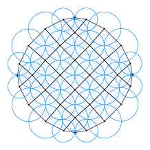
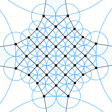
Figure 4. An orthogonal circle pattern and its dual. The boundary angles the dual pattern are $2\pi-\varphi_{i\!j}$ resp. $\pi-\varphi_{i\!j}$ depending on whether the degree of the boundary vertex is $3$ or $2$.

Now let us go back to the one parameter family $\mathcal{R}^{\delta}$ of ring patterns defined in Cor. 2.5. To avoid that the radii go to infinity as $\delta\to\pm\infty$ we scale the entire pattern by $2e^{-|\delta|}$. So the radii of the one parameter family of ring patterns are:

$$r_{m,n}^{\delta}=2e^{-|\delta|}\sinh(\rho_{m,n}+\delta)\quad\text{and}\quad R_{m,n}^{\delta}=2e^{-|\delta|}\cosh(\rho_{m,n}+\delta).$$

In the limit $\delta\to\pm\infty$ the areas of the rings tend to zero and for the radii we have:

$$\lim_{\delta\to\pm\infty}r^{\delta}_{i} =\lim_{\delta\to\pm\infty}2e^{-|\delta|}\frac{1}{2}(e^{\rho_{i}+\delta}-e^{-\rho_{i}-\delta})=\pm e^{\pm\rho_{i}}\,,$$

$$\lim_{\delta\to\pm\infty}R^{\delta}_{i} =\lim_{\delta\to\pm\infty}2e^{-|\delta|}\frac{1}{2}(e^{\rho_{i}+\delta}+e^{-\rho_{i}-\delta})=e^{\pm\rho_{i}}.$$

Remark 3.0. (Limits on compact subsets). If the ring pattern $\mathcal{R}$ is infinite we consider the limits $\delta\to\pm\infty$ of the family $\mathcal{R}^{\delta}$ on any compact subset $G_{0}\subset G$ satisfying the same conditions as $G$, i.e. $G_{0}$ and $G_{0}^{*}$ are simply connected.

Limit $\delta\to+\infty$. For $\delta>-\min_{v_{i}\in G_{0}}\rho_{i}$ we have $\rho_{i}^{\delta}=\rho_{i}+\delta>0$ for all $v_{i}\in G_{0}$. So considering the limit as $\delta\to\infty$ all $\rho^{\delta}_{i}$ will be positive and the angles of the circle pattern $\mathcal{C}$ (equation (5)) are exactly those of the ring pattern $\mathcal{R^{\delta}}$ given in Lemma 2.3. Furthermore, for $\delta\to\infty$, we obtain rings with area $0$ since the outer and inner radii both converge to $e^{\rho_{i}}$. The neighboring circles intersect orthogonally because inner and outer circles of the orthogonal ring pattern are intersecting orthogonally in the entire one parameter family. The limit circles form a Schramm type orthogonal circle pattern.

Limit $\delta\to-\infty$. For $\delta<-\max_{v_{i}\in G_{0}}\rho_{i}$ all $\rho_{i}^{\delta}=\rho_{i}+\delta<0$. By Lemma 2.3 the angles of the ring pattern for negative $\rho_{i}$ are given by

$$\varphi_{i\!j}=-2\arctan(e^{\rho_{i}-\rho_{j}})=-\pi+\arctan(e^{(-\rho_{i})-(-\rho_{j})})$$

and correspond to the angles of the dual pattern $\mathcal{C}^{*}$ with opposite orientation. As equation (4) is satisfied for all $\delta$, we obtain the dual orthogonal circle pattern $\mathcal{C}^{*}$ (with opposite orientation) in the limit.

Corollary 3.1.

Let $\mathcal{R}^{\delta}$ be a one parameter family of orthogonal ring patterns with $\rho^{\delta}_{i}=\rho_{i}+\delta$ for $\rho_{i}\in{\mathbb{R}}$ as described in Cor. 2.5. Then for $\delta\to+\infty$ we obtain an orthogonal circle pattern $\mathcal{C}$ with logarithmic radii $\rho_{i}$ and for $\delta\to-\infty$ we obtain the dual circle pattern $\mathcal{C}^{*}$ with logarithmic radii $-\rho_{i}$.

Here the limits are understood in the sense of Remark 3.0.

For a better understanding of the deformation, the one parameter family of cyclic quadrilaterals associated to a single edge $(v_{i},v_{j})$ is shown in Fig. 5: Assume that $\rho_{i}$ and $\rho_{j}$ are both positive and $\rho_{i}<\rho_{j}$. Then the deformation starts with an embedded cyclic quadrilateral (center right). For $\delta\to\infty$ we obtain two orthogonally intersecting circles with radii $e^{\rho_{i}}$ and $e^{\rho_{j}}$ that form a kite (bottom right). When $\delta\searrow-\rho_{i}$ one of the edges at $v_{i}$ shrinks to a point and reverses its direction as $\rho_{i}+\delta$ changes its sign from ${+}$ to ${-}$. If $-\rho_{j}<\delta<-\rho_{i}$ then $r_{i}^{\delta}<0$ and we obtain a non-embedded quadrilateral (top center). Again as $\delta\searrow-\rho_{j}$ one edge at $v_{j}$ shrinks to a point and changes its direction as $\rho_{j}+\delta$ changes sign (center left) and we obtain an embedded quadrilateral with negative orientation. For $\delta\to-\infty$ the areas of the rings go to zero and we obtain two orthogonally intersecting circles with radii $e^{-\rho_{i}}$ and $e^{-\rho_{j}}$ (bottom left).

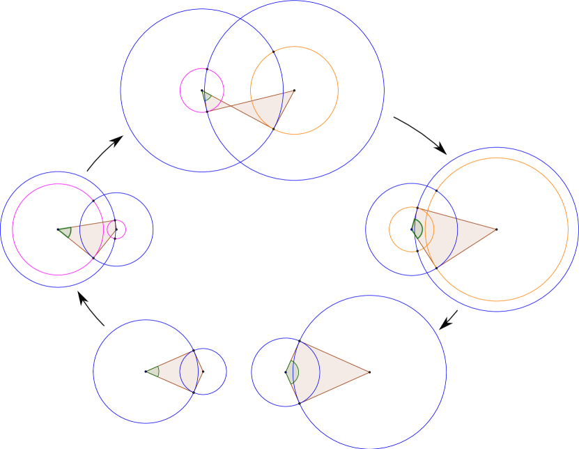
Figure 5. Deformation of a cyclic quadrilateral defined by two orthogonally intersecting rings. The bottom left and bottom right show the limits of the ring pattern as the area of the ring goes to zero. Positive radii are indicated by orange, negative radii (i.e., negative $\rho$) are indicated by pink circles. The angle associated with the left vertex is shown in green.

4. Doyle spiral, Erf, and $z^{\alpha}$ ring patterns

In this section we will have a look at some known orthogonal circle patterns and consider their ring pattern analogs and deformations.

4.1. Doyle spirals

Doyle spirals for the square lattice have been constructed by Schramm [6]. For $x+iy\in{\mathbb{C}}\setminus\{0\}$ Schramm defines radii by $r_{m,n}=|e^{(x+iy)(m+in)}|$. Taking the logarithm we obtain the logarithmic radii $\rho_{m,n}=mx-ny$. We will take these radii as a definition of the Doyle spiral ring pattern.

Proposition 4.1 (Doyle spiral ring pattern).

Let $x+iy\in{\mathbb{C}}\setminus\{0\}$ be a complex number. The Doyle spiral ring pattern is given by the $\rho$-radii $\rho_{m,n}=mx-ny$ for $(m,n)\in{\mathbb{Z}}^{2}$.

Let us consider the generic case $\frac{x}{y}\not\in{\mathbb{Q}}$ when the $\rho$-radii do not vanish. By Lemma 2.3 the angles of the cyclic quadrilaterals at the edges are given by

$$\varphi_{(m,n),(m+1,n)} =\begin{cases}\pi-2\arctan(e^{x})&\text{if $\rho_{m,n}>0$}\\ -2\arctan(e^{x})&\text{if $\rho_{m,n}<0$}\end{cases}\quad\text{and}$$

$$\varphi_{(m,n),(m,n+1)} =\begin{cases}\pi-2\arctan(e^{-y})&\text{if $\rho_{m,n}>0$}\\ -2\arctan(e^{-y})&\text{if $\rho_{m,n}<0$}\end{cases}$$

Looking closer at the signs of the $\rho$-radii we observe that

$$\rho_{m,n}>0 \Leftrightarrow mx>ny\, \rho_{m,n}<0 \Leftrightarrow mx<ny.$$ and

So the signs of the $\rho$-radii change across the line $\{(m,n)\in{\mathbb{Z}}^{2}\,|\,mx=ny\}$ and hence does the orientation of the flowers. If we restrict to the parts $\{(m,n)\in{\mathbb{Z}}^{2}\,|\,mx>ny\}$ (resp. $\{(m,n)\in{\mathbb{Z}}^{2}\,|\,mx<ny\}$) we see that the angles are constant for all horizontal edges $(m,n)(m+1,n)$ and all vertical edges $(m,n)(m,n+1)$. Thus we can define a Doyle spiral ring pattern by two angles $\alpha$ and $\beta$, one for the horizontal and one for the vertical direction. This is the characteristic property for the Doyle spiral circle pattern.

Consider the one parameter family $\mathcal{R}^{\delta}$ of orthogonal ring patterns as described by Cor. 2.5. The angles along the horizontal and vertical edges stay constant in the two halfspaces. As in the general case discussed in the previous section, all $\rho$’s become positive for $\delta\to+\infty$ (resp. negative for $\delta\to-\infty$), see Remark 3.0, and we obtain a Doyle spiral and its dual as constructed by Schramm (see Fig. 6).

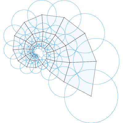
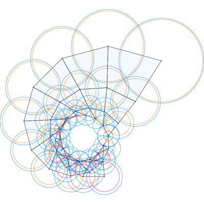
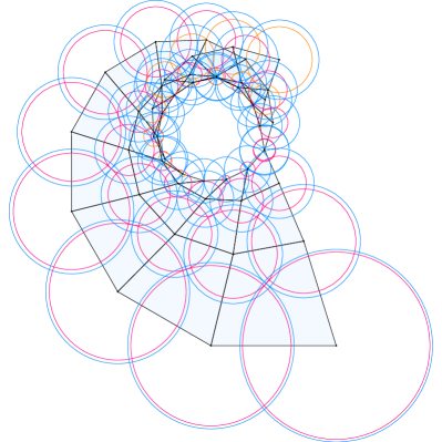
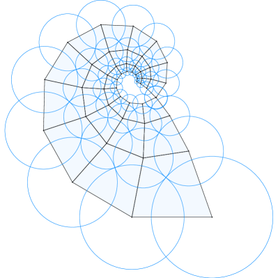
Figure 6. Deformation of an orthogonal circle pattern (top left) into its dual (bottom right) through a one parameter family of ring patterns (top right and bottom left). We see how the orientation of the quadrilaterals flips during the deformation. The innermost vertex in the top left circle patterns becomes the outermost vertex in the bottom right circle pattern.

4.2. Erf pattern

For analogs to Schramm’s $\sqrt{i}$-Erf pattern let us have a look at the corresponding radius function given in [6] $r_{m,n}=e^{amn}$ for $(m,n)\in{\mathbb{Z}}^{2}$ and $a\in{\mathbb{R}}$, $a>0$. Taking the logarithm we obtain $\rho_{m,n}=amn$. As in case of the Doyle spiral we will use this function to define the corresponding ring patterns.

Proposition 4.2 (Erf ring pattern).

Let $a\in{\mathbb{R}},a>0$. The Erf ring pattern is given by the $\rho$-radii $\rho_{m,n}=amn$ for $(m,n)\in{\mathbb{Z}}^{2}$.

The angles in the pattern are given by

$$\varphi_{(m,n),(m+1,n)} =\begin{cases}\pi-2\arctan(e^{-an})&\text{if $\rho_{m,n}>0$}\\ -2\arctan(e^{-an})&\text{if $\rho_{m,n}<0$}\end{cases}\quad\text{and}$$

$$\varphi_{(m,n),(m,n+1)} =\begin{cases}\pi-2\arctan(e^{-am})&\text{if $\rho_{m,n}>0$}\\ -2\arctan(e^{-am})&\text{if $\rho_{m,n}<0$}\end{cases}$$

As $\rho_{m,n}=amn$ the $\rho$-radii change signs at the coordinate axes. In the four quadrants, the angles along the horizontal and the vertical parameter lines are constant. All the rings on the coordinate axes are congruent: the radii of their outer circles are equal to $R=\cosh 0=1$, and their inner circles degenerate to their centers.

If we consider the one parameter family of ring patterns defined in Cor. 2.5 we see that in the limit $\delta\to+\infty$ we obtain the $\sqrt{i}$-SG Erf circle patterns constructed by Schramm. For $\delta\to-\infty$ we obtain a pattern with $\rho^{*}_{m,n}=-amn$. This is the same pattern as for $a$ since $\rho^{*}_{m,n}=\rho_{-m,n}$.

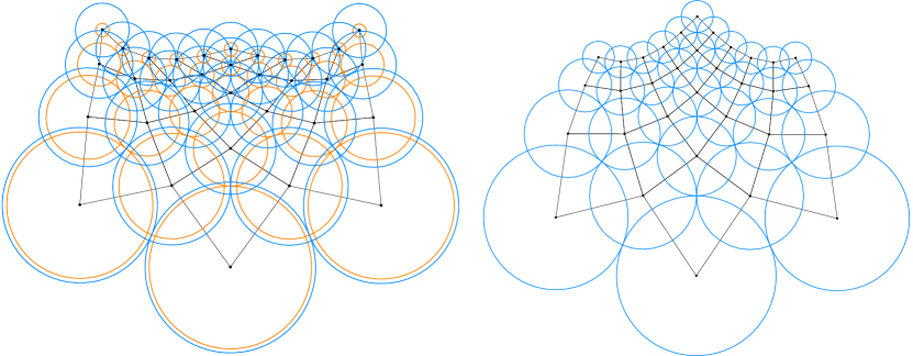
Figure 7. An Erf ring pattern (left) and the corresponding limit circle pattern.

4.3. $z^{\alpha}$ and logarithm patterns

In [2] the authors defined an orthogonal circle pattern $\mathcal{C}(z^{\alpha})$ as a discretization of the complex map $z\mapsto z^{\alpha}$ for $\alpha\in(0,2)$. The radius function of the circle pattern is given by the following identities (cf. [2, Thm. 3, equation (10, 11)]) on a subset of ${\mathbb{Z}}^{2}$ given by $V=\{(m,n)\,|\,m\geq|n|\}$:

$$r_{m,n}r_{m+1,n}(-2n-\alpha)+r_{m+1,n}r_{m+1,n+1}(2(m+1)-\alpha)\\ +r_{m+1,n+1}r_{m,n+1}(2(n+1)-\alpha)+r_{m,n+1}r_{m,n}(-2m-\alpha)=0$$

for $V\cup\{(-m,m-1)\,|\,m\in{\mathbb{N}}\}$ and

$$(m+n)(r_{m,n}^{2}-r_{m+1,n}r_{m,n-1})(r_{m,n+1}+r_{m+1,n})\\ +(n-m)(r_{m,n}^{2}-r_{m,n+1}r_{m+1,n})(r_{m+1,n}+r_{m,n-1})=0$$

for interior vertices $V\setminus\{(\pm m,m)\,|\,m\in{\mathbb{N}}\}$ with initial condition $r_{0,0}=1$ and $r_{1,0}=r_{0,1}=\tan\frac{\alpha\pi}{4}$.

It is known that the dual pattern of $z^{\alpha}$ is given by $z^{2-\alpha}$, e.g., the dual circle pattern of $\mathcal{C}(z^{2/3})$ is $\mathcal{C}(z^{4/3})=(\mathcal{C}(z^{2/3}))^{*}$ shown in Fig. 8 (top left and bottom right). Based on the logarithmic radii of these patterns we construct a one parameter family of ring patterns that interpolates between the two patterns.

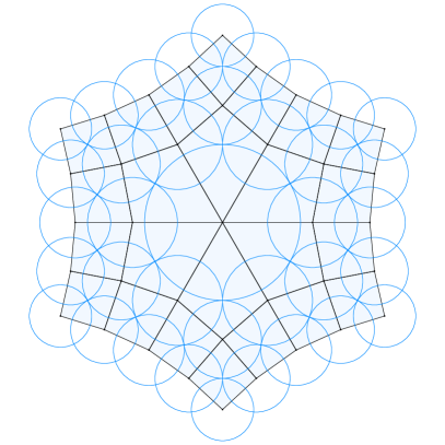
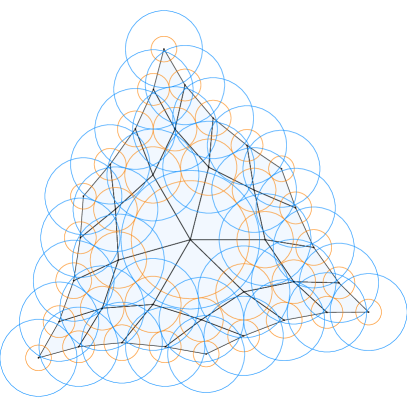
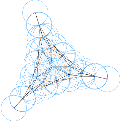
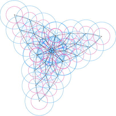
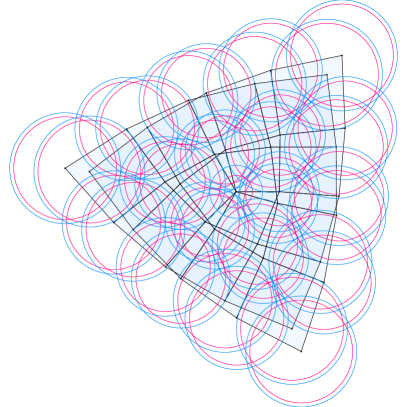
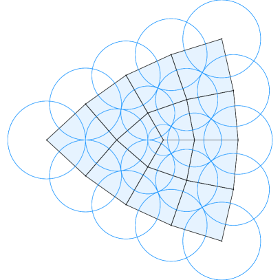
Figure 8. One parameter family of orthogonal ring patterns interpolating between the orthogonal circle pattern for $z\mapsto z^{2/3}$ (top left) and the dual pattern for $z^{4/3}$ (bottom right)

An orthogonal circle pattern for $z^{2}$ can be defined by considering a special limit for $\alpha\to 2$. The radii of the $z^{2}$ pattern are defined in [2, Sect. 5]. The dual of $z^{2}$ is the logarithm map $\log z$. In each of the corresponding orthogonal circle patterns, one of the circles degenerates. In case of $z^{2}$ one of the circles has radius $0$, i.e., the circle degenerates to a point and the logarithmic radius is negative infinity. Consequently, one of the circles in the $\log z$ pattern has radius infinity, i.e., the circle degenerates to a line and the logarithmic radius is positive infinity. We illustrate the one parameter deformation of $z^{2}$ to $\log(z)$ in Fig. 9.

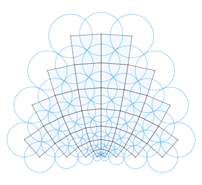
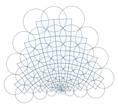
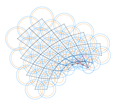
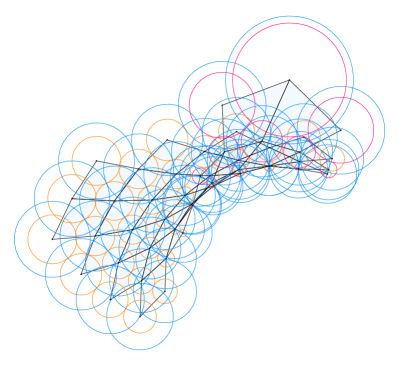
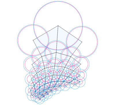
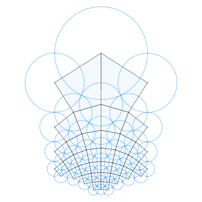
Figure 9. Orthogonal ring patterns interpolating between the circle patterns for $z^{2}$ and its dual pattern for $\log z$.

5. Variational description

The construction of a ring pattern is very similar to the construction of an orthogonal circle pattern since the equations at the interior vertices are the same (see Thm. 2.4). For (not necessarily orthogonal) circle patterns there exists a convex variational principle [5]. For planar orthogonal circle patterns the functional is given in terms of the logarithmic radii by:

$$S(\rho)=\sum_{v_{i}\bullet-\bullet v_{j}}\left(\operatorname{Im}\operatorname{Li}_{2}(ie^{\rho_{j}-\rho_{i}})+\operatorname{Im}\operatorname{Li}_{2}(ie^{\rho_{i}-\rho_{j}})-\frac{\pi}{2}(\rho_{i}+\rho_{j})\right)+\sum_{v_{i}}\Phi_{i}\rho_{i},$$

where the first sum is taken over all edges and the second sum over all vertices of $G$, $\operatorname{Li}_{2}$ is the dilogarithm function, $\operatorname{Im}\operatorname{Li}_{2}(ie^{x})=\int_{-\infty}^{x}\arctan e^{u}du$.

This functional is invariant with respect to the shift

(6) $$\rho_{i}\to\rho_{i}+h,\quad\forall i$$

if and only if

(7) $$\sum_{i}\Phi_{i}=\pi|E(G)|,$$

where $|E(G)|$ is the number of edges of $G$. The critical points are given by

(8) $$\frac{\partial S}{\partial\rho_{i}}=\Phi_{i}+\sum_{j:v_{j}{\bullet-\bullet}v_{i}}\left(2\arctan(e^{\rho_{i}-\rho_{j}})-\pi\right)=0.$$

The second derivative

$$D^{2}S=\sum_{v_{i}\bullet-\bullet v_{j}}\frac{1}{\cosh(\rho_{i}-\rho_{j})}(d\rho_{i}-d\rho_{j})^{2}$$

is positive for all variations different from (6).

Denote by $V_{B}$ the set of boundary vertices of $G$, i.e. the vertices with less then four neighbors. For simplicity consider ring patterns with positively oriented rings for all boundary vertices, i.e. on $V_{B}$ the function $\rho$ takes positive values. Equations (8) with

(9) $$\Phi_{i}=\begin{cases}2\pi&\text{for interior vertices}\\ \Theta_{i}&\text{for (positively oriented) boundary vertices}.\end{cases}$$

coincide with the orthogonal ring patterns equations (4).

Proposition 5.1.

Orthogonal ring patterns can be obtained as solutions of the following boundary valued problems:

• (Dirichlet boundary conditions) For any choice of prescribed radii $\rho:V_{B}\to{\mathbb{R}}_{+}$ of boundary rings there exists a unique orthogonal ring pattern $\mathcal{R}$.

• (Neumann boundary conditions) For any choice of boundary cone angles $\Theta:V_{B}\to{\mathbb{R}}_{+}$ satisfying (7) there exists a one parameter family of orthogonal ring patterns ${\mathcal{R}}_{h}$. The parameter $h$ is given by the shift (6). There exists $h_{0}$ such that for all $h>h_{0}$ all boundary rings of the ring pattern ${\mathcal{R}}_{h}$ are positively oriented.

Proof.

The existence and uniqueness of the boundary valued problems for orthogonal ring patterns can be treated exactly in the same way as for circle patterns. The later problems in a more general case were investigated in [5]. The existence and uniqueness for ring patterns follow from the convexity of the functional $S(\rho)$, for all variations different from (6). This also gives a way to compute the ring patterns by minimizing the functional. For the Neumann boundary valued problem one varies $\rho$’s at all vertices $V(G)$. The condition (7) implies that the solutions possess the symmetry group (6) described in Section 3. ∎

An example of solution of a Neumann boundary value problem is presented in Fig. 10). Here for all interior vertices $\Phi=2\pi$, for all boundary and not corner vertices $\Phi_{i}=\Theta_{i}=\pi$. Four angles $\Phi_{i}=\Theta_{i}$ at corner vertices of the quadrilateral should sum up to $2\pi$. One can easily check that the last condition implies (7).

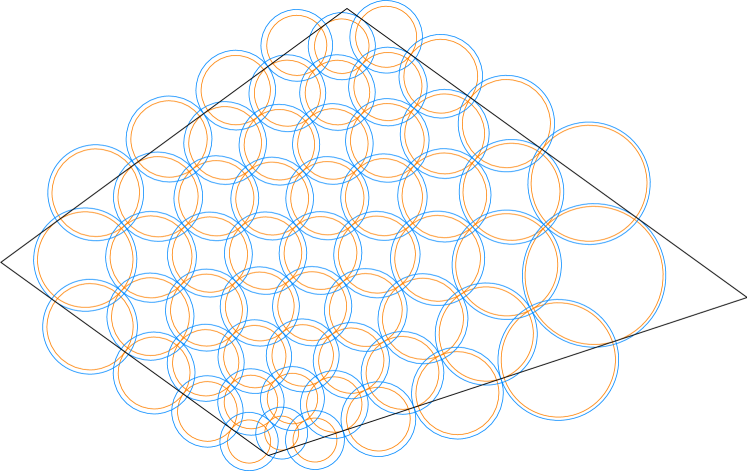
Figure 10. An orthogonal ring pattern computed using the variational principle with Neumann boundary conditions. The prescribed angles are $\pi$ for the boundary vertices of degree $2$. The shape is governed by the four angles, with the sum $2\pi$, prescribed for the four corner boundary vertices of degree $1$.

Acknowledgements

We thank Boris Springborn for fruitful discussions on circle patterns and variational principles and Nina Smeenk for the support in developing the software for creating the figures. We also thank the anonymous referee for valuable suggestions which improved the presentation.

References

- [1] V. E. Adler, A. I. Bobenko, and Y. B. Suris. Classification of integrable equations on quad-graphs. The consistency approach. Comm. Math. Phys., 233(3):513–543, 2003.
- [2] S. I. Agafonov and A. I. Bobenko. Discrete and Painlevé equations. International Mathematics Research Notices, 2000(4):165–193, 01 2000.
- [3] A. I. Bobenko and T. Hoffmann. S–conical cmc surfaces. Towards a unified theory of discrete surfaces with constant mean curvature. In A. I. Bobenko, editor, Advances in Discrete Differential Geometry. Springer, 2016.
- [4] A. I. Bobenko, U. Pinkall, and B. A. Springborn. Discrete conformal maps and ideal hyperbolic polyhedra. Geom. Topol., 19(4):2155–2215, 2015.
- [5] A. I. Bobenko and B. A. Springborn. Variational principles for circle patterns and Koebe’s theorem. Trans. Amer. Math. Soc., 356(2):659–689, 2004.
- [6] O. Schramm. Circle patterns with the combinatorics of the square grid. Duke Math. J., 86(2):347–389, 1997.
- [7] X. Tellier, L. Hauswirth, C. Douthe, and O. Baverel. Discrete CMC surfaces for doubly-curved building envelopes. In L. Hesselgren, A. Kilian, S. M. andKarl Gunnar Olsson, and O. S.-H. C. Williams, editors, Advances in Architectural Geometry, 2018.