AETv2: AutoEncoding Transformations for Self-Supervised Representation Learning by Minimizing Geodesic Distances in Lie Groups

Abstract

Self-supervised learning by predicting transformations has demonstrated outstanding performances in both unsupervised and (semi-)supervised tasks. Among the state-of-the-art methods is the AutoEncoding Transformations (AET) by decoding transformations from the learned representations of original and transformed images. Both deterministic and probabilistic AETs rely on the Euclidean distance to measure the deviation of estimated transformations from their groundtruth counterparts. However, this assumption is questionable as a group of transformations often reside on a curved manifold rather staying in a flat Euclidean space. For this reason, we should use the geodesic to characterize how an image transform along the manifold of a transformation group, and adopt its length to measure the deviation between transformations. Particularly, we present to autoencode a Lie group of homography transformations ${\bf PG}(2)$ to learn image representations. For this, we make an estimate of the intractable Riemannian logarithm by projecting ${\bf PG}(2)$ to a subgroup of rotation transformations ${\bf SO}(3)$ that allows the closed-form expression of geodesic distances. Experiments demonstrate the proposed AETv2 model outperforms the previous version as well as the other state-of-the-art self-supervised models in multiple tasks.

1 Introduction

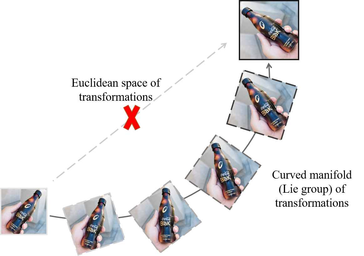
Figure 1: The deviation between two transformations should be measured along the curved manifold (Lie group) of transformations rather than through the forbidden Euclidean space of transformations.

Learning powerful representations from data is one of the most significant topics in many deep learning problems. In particular, self-supervised representation learning from transformed images has shown great potential in both unsupervised and (semi-)supervised tasks, where the backbone networks are trained and regularized by decoding the self-supervisory signals without involving supervised labels [18, 10]. These representations learned from transformations have also been well connected with the transformation equivariant representations as they change equivariantly in the same way as images are transformed.

The state-of-the-art performances have been demonstrated in literature for the transformation-based representation learning. Among them is the paradigm of AutoEncoding Transformations (AET) [23, 17] that extends the family of autoencoders in a novel way. The idea is straightforward based on a simple criterion: a powerful representation should be able to capture the intrinsic visual structures of images before and after a transformation, such that the transformation can be well decoded from the representations of original and transformed images. In other words, the transformations are used as a critical weapon to reveal the intrinsic pattern of visual structures that change equivariantly to the applied transformations. Both deterministic and probabilistic AET models have been presented in literature, which minimizes the Mean-Square Errors (MSE) between the matrix representation of parametric transformations and maximizes the mutual information between the learned representation and transformations, respectively.

Although both AET models have shown the promising results, both the MSE and information maximization criteria suffer a questionable assumption that the Euclidean distance between transformation matrices is a good metric to characterize the difference between the estimation and the groundtruth. Unfortunately, this assumption is unrealistic. A group of transformations have a restricted form of the matrix representation on a manifold rather than scattering in the ambient Euclidean space of matrices. This suggests that a valid path connecting two transformations cannot be a straight line in the Euclidean space of transformation matrices. Instead it should be the shortest curve along the manifold of transformations, i.e., a geodesic.

This is illustrated in Figure 1. In other words, given a pair of original and transformed images, one cannot find a valid sequence of transformation matrices in the Euclidean space to continuously transform the original one to its transformed counterpart. Instead, a valid shortest path of transformations can only be sought on the manifold of the transformation group. This suggests that a more meaningful metric is the geodesic distance between two transformations defined along the underlying manifold.

Therefore, we resort to the theory of Lie group to study the geometry of transformations on the underlying manifold. We will formally present a new criterion to train the AET model by minimizing the geodesic distance between the estimated and applied transformations. In particular, we will use the homography group ${\bf PG}(2)$ to train the AET model, which contains a rich composition of image transformations such as rotations, translations and projective transformations. While Riemannian logarithm is needed to characterize the geodesic distance between transformations, its calculation is intractable in the homography group without a closed form. To this end, we choose to project the transformations onto a subgroup with a tractable expression of geodesic distances. In particular, we will show that the rotation group ${\bf SO}(3)$ is a subgroup of ${\bf PG}(2)$, where the geodesic distance and its derivative can be efficiently computed to train the model without having to explicitly take the logarithm. This can greatly reduce the computing overhead in self-training the proposed AETv2 model with the Lie group of homography transformations.

The remainder of this paper is organized as follows. In the next section, we will introduce some background about the transformation-based representation learning and point out its drawback. Then, the criterion of geodesic distance minimization will be proposed to train the AETv2 in Section 3, following a brief discussion of the preliminaries about the theory on the Lie group of transformations. We will discuss the implementation details about applying the homography group to train the proposed AETv2 model in Section 4. Experiment results will be demonstrated in Section 5, and we will conclude in Section 6.

2 Background and Notations

First, let us review the previous work on Auto-Encoding Transformations (AET) [23], as well as discuss its drawback that will be addressed in this paper.

In the AET, a transformation $\mathbf{t}$ is sampled from a group $\mathcal{G}$, which is then applied to an image $\mathbf{x}$, resulting in a transformed copy $\mathbf{t}(\mathbf{x})$. Usually, a transformation $\mathbf{t}$ can be represented by the corresponding matrix $\mathbf{T}$ in a group. For example, for the group ${\rm SIM}(2)$ of 2D similarity transformations, a transformation can be represented by a $3\times 3$ matrix $\mathbf{T}$ that is applied to a homogeneous space of coordinates to transform images spatially.

The goal of the AET is to learn a representation encoder $E(\mathbf{x})$ for an image $\mathbf{x}$, as well as a transformation decoder $D$ to estimate the transformation $\mathbf{t}$ from the representations $E(\mathbf{x})$ and $E(\mathbf{t}(\mathbf{x}))$ of original and transformed images.

It is supposed that a good representation encoder $E$ can capture the intrinsic visual structures of individual images, so that the decoder can infer the applied transformation by comparing the encoded representations of images before and after the transformations. Recent work has revealed the relation between the AET model and the transformation-equivariant representations from an information-theoretic point of view [18].

Formally, to learn the encoder $E$ and the decoder $D$, the following Mean-Squared Error (MSE) is minimized to train the AET model with weights $\Theta$

$$\bf\min_{\Theta}\mathop{\mathbb{missing}}E\limits_{\mathbf{x},\mathbf{t}}{\rm\dfrac{1}{2}}\|{\hat{T}}(\Theta)-T\|^{2}_{\rm F}$$ (1)

where $\|\cdot\|_{\rm F}$ is the Frobenius norm of matrix, $\bf\hat{T}$ is an estimate of the matrix representation $\mathbf{T}$ of the sampled transformation $\mathbf{t}$, which is a function of the model parameters $\Theta$, and the mean-squared error is taken over the sampled images $\mathbf{x}$ and transformations $\mathbf{t}$.

Although the previous empirical results showed impressive performances of the learned AET representations, the above objective may not exactly characterize the distance between the estimate and the sampled transformation, as it simply uses the Euclidean distance between the matrix representations.

Indeed, a transformation group $\mathcal{G}$ is embedded into the ambient matrix space, thereby forming a manifold called a Lie Group. Obviously, a more accurate distance between two transformations should be characterized by the length of the geodesic connecting them, which characterizes how a transformation can continuously change to another transformation along the underlying manifold. Minimizing such a geodesic distance on the manifold can yield a more exact estimate of a sampled transformation along the Lie group of transformations.

3 The Proposed Approach

In this section, we will briefly review the background knowledge about the Lie group in Section 3.1. Then we will define the Geodesic Distance between Transformations (GDT) in Section 3.2, and present the training of the AET model by minimizing the GDT in Section 3.3.

3.1 Preliminaries

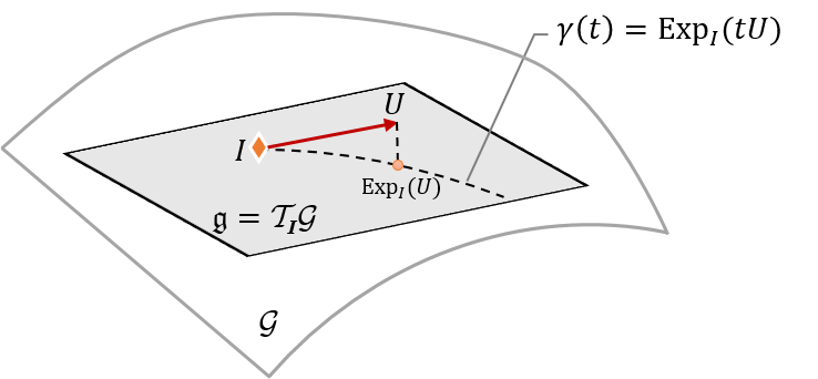
Figure 2: Illustration of a Lie group $\mathcal{G}$ of transformations with its Lie algebra $\mathfrak{g}$ as the tangent space $\bf\mathcal{T}_{I}\mathcal{G}$ at the identity $\mathbf{I}$. A geodesic curve $\rm\gamma(t)$ is defined by the Riemannian exponential $\bf{\rm Exp}_{I}(\mathrm{t}U)$ with the velocity $\mathbf{U}\in\mathfrak{g}$ at $\mathbf{I}$, where the Riemannian exponential $\bf{\rm Exp}_{I}$ maps $\bf U$ to the Lie group $\mathcal{G}$.

As illustrated in Figure 2, a Lie group $\mathcal{G}$ of transformations is both a group and a manifold [21]. As a group, it is endowed with a composition $\circ$ and an inverse operator, which become the matrix product and inverse in the corresponding matrix representation. For simplicity, we will use the matrix representation of transformations in the following exposition.

As a manifold, the tangent space $\mathcal{T}_{\mathbf{I}}\mathcal{G}$ at the identity transformation $\mathbf{I}$ plays a critical role, which is named the Lie algebra $\mathfrak{g}$ in literature [21]. It is a linear vector space endowed with the matrix addition and scalar multiplication. A group exponential $\exp$ is defined by mapping from the Lie algebra $\mathfrak{g}$ to the Lie group $\mathcal{G}$. In the matrix representation, the group exponential becomes matrix exponential [21].

Besides the group exponential, when a Riemannian metric is defined on the manifold of Lie group, a geodesic $\gamma({\rm t}):[0,1]\rightarrow\mathcal{G}$ can be defined starting from the identity transformation $\gamma(0)=\mathbf{I}$ with an initial velocity $\gamma^{\prime}(0)=\mathbf{U}\in\mathfrak{g}$. Then the Riemannian exponential is defined as ${\rm Exp}_{\mathbf{I}}(\mathbf{U})\triangleq\gamma(1)$. Note that the Riemannian exponential ${\rm Exp}_{\mathbf{I}}$ does not necessarily coincide with the group exponential unless there exists a bi-invariant metric [21] on the Lie group.

The group exponential may not be surjective, i.e., it does not map the Lie algebra $\mathfrak{g}$ onto the whole Lie group $\mathcal{G}$. In contrast, the Riemannian exponential is a surjective mapping onto a connected $\mathcal{G}$. This implies there exists a Riemannian logarithm ${\rm Log}_{\mathbf{I}}$ mapping from $\mathcal{G}$ back to $\mathfrak{g}$ such that $\bf{\rm Exp}_{I}({\rm Log}_{I}(U))=U$.

Usually, we consider a left-invariant Riemannian metric $\bf\langle U,V\rangle_{T}$ on the Lie group $\mathcal{G}$ for $\bf U,V\in\mathcal{T}_{T}\mathcal{G}$, satisfying $\bf\langle U,V\rangle_{T}=\langle T^{-1}U,T^{-1}V\rangle_{I}$. Thus, one only needs to define an inner product on the Lie algebra $\mathfrak{g}$, and the inner product in the tangent space at the other transformations can be translated from that at the identity [21]. The left-invariant metric preserves the length of geodesics under a left translation by $\mathbf{T}$ (i.e., $\bf X\mapsto TX$ for each $\bf X\in\mathcal{G}$). Therefore, the Riemannian exponential ${\rm Exp}_{\mathbf{T}}$ at any transformation $\mathbf{T}$ can be written as $\bf{\rm Exp}_{T}(U)=T~{}{\rm Exp}_{I}(T^{-1}U)$ for $\bf U\in\mathcal{T}_{T}\mathcal{G}$.

3.2 Geodesic Distance between Transformations

In the AET, we seek to train the model by minimizing the error between the estimated and sampled transformations $\bf\hat{T}$ and $\bf T$. In the previous work, the mean-squared distance (aka the squared Euclidean distance) is adopted. However, it does not reflect the intrinsic distance between transformations along the manifold of the underlying Lie group. In contrast, it is only the external distance between the transformations in the ambient Euclidean space for matrices.

Thus, we instead use the geodesic to connect two transformations, which has the shortest length along the curved manifold between them. With the above discussion, it can be shown that the geodesic connecting $\bf\hat{T}$ and $\bf T$ can be represented as

$$\bf\gamma({\rm t})={\rm Exp}_{T}({\rm t}~{}{\rm Log}_{T}(\hat{T}))=T{\rm Exp}_{I}({\rm t}~{}{\rm Log}_{I}(T^{-1}\hat{T}))$$

where $\gamma(0)=\mathbf{T}$ and $\gamma(1)=\bf\hat{T}$. Then, the geodesic distance between $\mathbf{T}$ and $\bf\hat{T}$ is defined as

$$\rm\int_{0}^{1}\|\gamma^{\prime}(t)\|dt=\int_{0}^{1}\sqrt{\langle\gamma^{\prime}(t),\gamma^{\prime}({\rm t})\rangle_{\gamma(t)}}dt=\|\gamma^{\prime}(0)\|$$

since $\gamma^{\prime}(\rm t)$ is parallel along $\gamma(\rm t)$ and thus $\|\gamma^{\prime}(\rm t)\|$ is a constant along the geodesic.

Therefore, we can minimize the following (squared) Geodesic Distance between Transformations (GDT) to train the AET model

$$\bf\ell(\hat{T},T)\triangleq{\rm\dfrac{1}{2}}\|\gamma^{\prime}({\rm 0})\|^{\mathrm{2}}={\rm\dfrac{1}{2}}\|{\rm Log}_{I}(T^{-1}\hat{T})\|^{\mathrm{2}}$$ (2)

where the last equality follows from the left invariance of the Riemannian metric.

3.3 Autoencoding Transformations in Lie Groups

In the AET, $\bf\hat{T}$ in the loss (2) is the estimate of a sampled transformation $\bf T$ by the transformation decoder. Let a residual matrix $\bf R$ be $\bf{\rm Log}_{I}(T^{-1}\hat{T})$. Then, we can rewrite the geodesic distance between $\bf\hat{T}$ and $\mathbf{T}$ as

$$\bf\ell(\hat{T},T)={\rm\dfrac{1}{2}}{\rm tr}(R^{\intercal}R)$$ (3)

where

$$\bf{\rm Exp}_{I}(R)=T^{-1}\hat{T}.$$ (4)

Here $\mathbf{R}$ is viewed as a function of the estimation $\bf\hat{T}$ that further depends on the weights of the AET network.

In order to train the model via error back-propagation, we need to compute the derivative of $\bf\ell(\hat{T},T)$ wrt $\bf\hat{T}$. By applying the chain rule of Fr$\acute{e}$chet matrix derivative wrt $\bf\hat{T}$ to LHS of (4), we have

$$\bf\nabla_{\hat{T}}{\rm Exp}_{I}(R)=\nabla_{R}{\rm Exp}_{I}(R)\nabla_{\hat{T}}R$$

On the other hand, the derivative of the RHS of (4) is

$$\bf\nabla_{\hat{T}}(T^{-1}\hat{T})=I\otimes T^{-1}.$$

By equating the above two results, we obtain

$$\bf\nabla_{\hat{T}}R=(\nabla_{R}{\rm Exp}_{I}(R))^{-1}I\otimes T^{-1}$$

where $\otimes$ is the Kronecker product, and $\bf I$ is the identity matrix with a compatible dimension in the matrix product.

By following the chain rule, one can write the derivative of the objective $\ell$ wrt the decoder output $\bf\hat{T}$

$$\bf\nabla_{\hat{T}} \bf\ell(\hat{T},T)=\overline{R}^{\intercal}~{}\nabla_{\hat{T}}R$$ (5)

$$\bf=\overline{R}^{\intercal}~{}(\nabla_{R}{\rm Exp}_{I}(R))^{-1}I\otimes T^{-1}$$

where the overline $\bf\overline{R}$ denotes the stacking of the matrix columns. With the above derivative, the error signals will be back-propagated to update the network parameters.

In the next section, we will implement the AET with the group of homography transformations. We will discuss the challenge of directly computing its Riemannian exponential $\bf\bf{\rm Exp}_{I}$ and the corresponding (Fr$\acute{e}$chet) matrix derivative, and present an alternative tractable algorithm.

4 The Implementation

In this section, we will discuss the implementation details about the proposed approach. First, we will review the Lie group of homography transformations in Section 4.1, and show the challenge facing the direct application of Riemannian logarithm to compute the geodesic distance between transformations. Then, we will present an alternative algorithm in Section 4.2 by projecting the homography group onto a subgroup where there exists a tractable form of geodesic distance without explicitly computing the intractable Riemannian logarithm.

4.1 Homography Transformations

The previous results have demonstrated that the group ${\rm\bf PG}(2)$ of homography transformations (aka projective transformations) have gained impressive performances with the AET model (referred to AETv1 in this paper) [23]. It contains a rich family of spatial transformations that can reveal the visual structures of images. Thus, we discuss the details about implementing the proposed AETv2 with ${\rm\bf PG}(2)$ below.

The 2D homography transformations ${\rm\bf PG}(2)$ can be defined as the transformations in the augmented 3D homogeneous space of image coordinates [1]. Its matrix representation contains all matrices with a unit determinant, and the corresponding Lie algebra $\mathfrak{g}$ consists of all matrices with zero trace.

With a left-invariant metric, the Riemannian exponential can be written in terms of matrix exponential [21],

$$\bf{\rm Exp}_{I}(R)=\exp(R^{\intercal})\exp(R-R^{\intercal})$$

for all $\bf R\in\mathfrak{g}$. By applying the chain rule, the matrix derivative of $\bf{\rm Exp}_{I}$ can be rewritten as

$$\bf\nabla_{R} \bf{\rm Exp}_{I}(R)=\bf\exp(R^{\intercal}-R)\otimes I~{}{\rm d}\exp(R^{\intercal})K$$ (6)

$$\bf+I\otimes\exp(R^{\intercal})~{}{\rm d}\exp(R-R^{\intercal})(I-K)$$

where ${\rm d}\exp$ is the derivative of matrix exponential, and $\bf K$ is the communication matrix such that $\bf K\overline{M}=\overline{M^{\intercal}}$ for a matrix $\bf M$.

Then, substituting (6) in (5) results in the derivative of the loss (3) wrt the estimated transformation $\bf\hat{T}$, which can be back-propagated to train the model.

4.2 Projection of ${\bf PG}(2)$ onto ${\bf SO}(3)$

The derivative in Eq. (5) involves the calculation of Riemannian logarithm $\mathbf{R}$ of $\bf T^{-1}\hat{T}$. Unfortunately, there is no closed-form solution to this Riemannian logarithm, and an optimization problem need be formulated to solve it by inverting the Riemannian exponential.

Here we present an alternative method by projecting the target transformation $\bf T^{-1}\hat{T}$ onto a subgroup, where there exists a tractable Frobenius norm of Riemannian logarithm [22]. For the homography group ${\bf PG}(2)$, the rotation group ${\bf SO}(3)$ constitutes a subgroup by noting that its matrix representation consists of such $3\times 3$ matrices that $\bf T^{\intercal}T=I$ and $\det(\mathbf{T})=1$, and the corresponding Lie algebra contains all skew-symmetric matrices (i.e., $\bf R^{\intercal}=-R$) with traces equal to zero [21]. The Riemannian logarithm for the rotation subgroup is the matrix logarithm since the matrices commute in its Lie algebra.

Formally, an estimate of $\bf R$ can be made by projecting onto ${\bf SO}(3)$ and using the matrix logarithm in place of the Riemannian logarithm,

$$\bf\hat{R}=\log\left[{\rm\mathop{\Pi}\limits_{{\bf SO}(3)}}(T^{-1}\hat{T})\right]$$

where $\log$ is the conventional matrix logarithm, and ${\rm\mathop{\Pi}\limits_{{\bf SO}(3)}}(\cdot)$ is the projection operator.

With the singular value decomposition of $\bf T^{-1}\hat{T}=U\Sigma V^{\intercal}$, it is not hard to show by the Karush-Kuhn-Tucker (KKT) conditions [3] that the projection onto ${\bf SO}(3)$ can be written in a closed form as

$$\bf P\triangleq{\rm\mathop{\Pi}\limits_{{\bf SO}(3)}}(T^{-1}\hat{T})=U{\rm diag}\left\{1,1,\det(UV^{\intercal})\right\}V^{\intercal}.$$

Moreover, by Rodrigues’ rotation formula [8], the Frobenius norm of the resultant $\bf\hat{R}\triangleq\bf\log P$ can be written as

$$\bf\dfrac{\rm 1}{\rm 2}\|\hat{R}\|_{\rm F}^{\rm 2}\triangleq{\rm\dfrac{1}{2}}{\rm tr}(\hat{R}^{\intercal}\hat{R})=\theta^{\rm 2},$$

where

$$\bf\theta=\arccos\left[\dfrac{{\rm tr}(P)-{\rm 1}}{\rm 2}\right]\in[{\rm 0},\pi]$$ (7)

is the rotation angle around a unit 3D axis given by $\theta^{-1}\log\mathbf{P}$ whenever $\theta\neq 0$.

Algorithm 1 Self-training the AETv2 with homography transformations

  Input: the model weights $\Theta$, minibatch size $n$

  repeat

     Sample $n$ unlabeled images $\mathcal{X}=\{\mathbf{x}_{i}|i=1,\cdots,n\}$;

     Sample $n$ transformations $\mathcal{T}=\{\mathbf{t}_{i}|i=1,\cdots,n\}$, and apply to $\mathcal{X}$, resulting in the set of transformed images $\mathcal{T}(\mathcal{X})=\{\mathbf{t}_{i}(\mathbf{x}_{i})|i=1,\cdots,n\}$;

     Use the gradient of the loss (8) over the minibatch

$$\dfrac{1}{n}\sum_{i=1}^{n}\nabla_{\Theta}\mathbf{\hat{\ell}}(\mathbf{\hat{T}}_{i},\mathbf{T}_{i})$$

to update the model weights $\Theta$, with $\mathbf{\hat{T}}_{i}$ and $\mathbf{T}_{i}$ the matrix representation of the decoder output and the applied transformation for the $i$th sample.

  until Convergence

Then, we can approximate the loss $\bf\ell(\hat{T},T)$ in Eq. (3) by combining the resultant geodesic distance and the distance between $\bf T^{-1}\hat{T}$ to its projection onto ${\bf SO}(3)$,

$$\bf\hat{\ell}(\hat{T},T)=\arccos\left[\dfrac{{\rm tr}(P)-{\rm 1}}{\rm 2}\right]+\lambda~{}{\rm tr}(R_{\Pi}^{\intercal}R_{\Pi})$$ (8)

with the following projection residual

$$\bf R_{\Pi}=T^{-1}\hat{T}-{\rm\mathop{\Pi}\limits_{{\bf SO}(3)}}(T^{-1}\hat{T}),$$

where $\lambda$ is a positive weight on the projection distance, and it will be fixed to one in experiments. Minimizing the projection residual can minimize the deviation incurred by projecting $\bf T^{-1}\hat{T}$ onto ${\bf SO}(3)$.

As illustrated in Figure 3, we choose to minimize the above loss as a tractable surrogate to train the AET model without having to explicitly taking the matrix logarithm. Since most of common libraries automate the gradient of both the SVD and the determinant, the derivative of the projection can be implemented directly. Algorithm 1 summarizes the algorithm of self-training the AETv2 with homography transformations.

5 Experiments

In this section, we present our experiment results by comparing the AETv2 with the AETv1 as well as the other unsupervised models. Following the standard evaluation protocol in literature [23, 18, 15, 7, 19, 14, 9], we will adopt downstream classification tasks to evaluate the learned representations on CIFAR10, ImageNet, and Places datasets.

5.1 Implementation Details

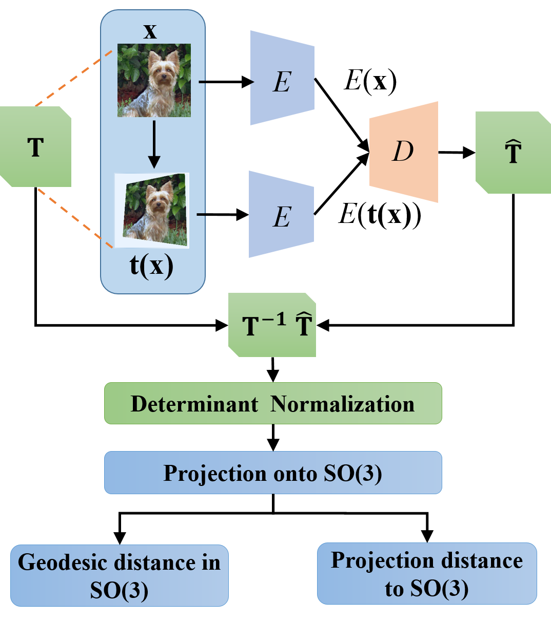
Figure 3: Illustration of how the AETv2 is self-trained end-to-end. The output matrix $\bf T^{-1}\hat{T}$ from the transformation decoder is normalized to have a unit determinant, and the projection of $\bf T^{\rm-1}\hat{T}$ onto ${\bf SO}(3)$ follows to compute the geodesic distance and the projection loss as in Eq. (8) to train the model.

As in the AETv1 [23], a backbone network architecture is adopted to train a representation encoder and a transformation decoder for the AETv2 network. As shown in Figure 3, an image and its transformed copy are fed into a Siamese encoder network, whose output representations are taken as the input into a transformation decoder. But unlike the AETv1, the AETv2 model works to decode the Lie group of homography transformations, and it outputs a matrix representation of the estimated transformations. Since a $3\times 3$ homography transformation matrix has eight degrees of freedom up to a scalar multiplier, its transformation matrix is obtained from the eight outputs by the decoder, with the last element fixed to one. The resultant transformation matrix $\bf T^{-1}\hat{T}$ is finally normalized to have a unit determinant as illustrated in Figure 3.

For the sake of a fair comparison, a homography transformation is sampled like in the AETv1 by randomly translating four corners of an image in both horizontal and vertical directions by $\pm 0.125$ of its height and width, after it is randomly scaled by $[0.8,1.2]$ and rotated by $0^{\circ},90^{\circ},180^{\circ},$ or $270^{\circ}$.

5.2 CIFAR-10 Experiments

5.2.1 Network and Experiment Details

To make a fair and direct comparison with existing unsupervised models, we adopt the Network-In-Network (NIN) architecture previously used on the CIFAR-10 dataset for the unsupervised learning task [23, 18, 15, 7, 19, 14, 9]. The NIN consists of four convolutional blocks, each having three convolutional layers. Two Siamese NIN branches are then constructed in the AETv2, each of which takes the original and the transformed images, respectively. The outputs from the last block of two branches are concatenated and average-pooled to form a $384$-d feature vector. An output layer follows to predict the eight parameters of the input homography transformation. The model is trained by the Adam solver with a learning rate of $10^{-5}$, a value of $0.9$ and $0.999$ for $\beta_{1}$ and $\beta_{2}$, and a weight decay rate of $5\times 10^{-4}$.

A classifier is then built on top of the second convolutional block to evaluate the quality of the learned unsupervised representation following the standard protocol in literature [23, 18, 15, 7, 19, 14, 9]. In particular, the first two blocks are frozen when the classifier atop is trained with labeled examples.

Both model-based and model-free classifiers are trained for the evaluation purpose. First, we train a non-linear classifier with various numbers of Fully-Connected (FC) layers. Each hidden layer has $200$ neurons followed by a batch-normalization and ReLU activation. We also train a convolutional classifier by adding a third NIN block on top of the unsupervised features, and its output feature map is averaged pooled and connected to a linear softmax layer.

Alternatively, we test a model-free KNN classifier based on the averaged-pooled features from the second convolutional block. Without explicitly training a model with labeled data, the KNN classifier can make a direct assessment on the quality of unsupervised feature representations.

5.2.2 Results

Table 1: Comparison between unsupervised models on CIFAR-10. The fully supervised NIN and the random Init. + conv have the same three NIN blocks, but they are fully supervised and is trained with the first two blocks randomly initialized and staying frozen during training, respectively. “+FC” and “+conv” denote a nonlinear classifier with a hidden FC layer and a NIN convolutional block respectively, followed by a 10-way softmax layer.

Method	Error rate
Supervised NIN (Lower Bound)	7.20
Random Init. + conv (Upper Bound)	27.50
Roto-Scat + SVM [15]	17.7
ExamplarCNN [7]	15.7
DCGAN [19]	17.2
Scattering [14]	15.3
RotNet + FC [9]	10.94
RotNet + conv [9]	8.84
AETv1 + FC [23]	9.41
AETv1 + conv [23]	7.82
(Ours) AETv2 + FC	9.09
(Ours) AETv2 + conv	7.44

Table 2: Comparison between AETv1 and AETv2 on CIFAR-10 with different classifiers on top of learned representations for evaluation, where $n$-FC denotes a $n$-layer fully connected (FC) classifier, and the KNN is obtained with $K=10$ nearest neighbors. The numbers in parentheses are the relative reduction in error rates w.r.t. the AETv1 baseline.

	KNN	1-FC	2-FC	3-FC	conv
AETv1 [23]	22.39	16.65	9.41	9.92	7.82
(Ours) AETv2	21.26 ($\downarrow$ 5.0%)	15.03 ($\downarrow$ 9.7%)	9.09 ($\downarrow$ 3.4%)	9.55 ($\downarrow$ 3.7%)	7.44 ($\downarrow$ 4.9%)

Table 1 compares the AETv2 with the other models on CIFAR-10. On one hand, it outperforms the AETv1 as well as the other unsupervised models with the same backbone. Furthermore, it narrows the performance gap with the fully supervised convolutional classifier ($7.44\%$ vs. $7.20\%$) that gives the lower bound of error rate when all labels are used to train the model end-to-end.

More comparisons with the AETv1 are made in Table 2. We compare the performances by both the model-based and model-free classifiers in the downstream tasks for both versions of the AET models. From the results, we can see that the AETv2 consistently outperforms its AETv1 counterpart with both KNN classifiers and different numbers of fully connected layers.

5.3 ImageNet Experiments

5.3.1 Network and Experiment Details

We further evaluate the performance on the ImageNet dataset. For a fair comparison with the AETv1 [23], the AlexNet is used as the backbone to learn the unsupervised features. Two branches with shared parameters are created by taking original and transformed images as inputs to train the unsupervised model. The $4,096$-d output features from the second last fully connected layer in two branches are concatenated and fed into the output layer producing eight projective transformation parameters. We still use the Adam solver to train the network with a batch size of $768$ original and transformed images.

5.3.2 Results

Table 3: Top-1 accuracy on ImageNet. After unsupervised training of AlexNet, nonlinear classifiers are trained on top of Conv4 and Conv5 layers with labeled data for the evaluation purpose. The fully supervised and random models are also compared that give upper and lower bounded performances, respectively. A single crop is applied with no dropout or local response normalization during the testing.

Method	Conv4	Conv5
ImageNet Labels [2](Upper Bound)	59.7	59.7
Random [13] (Lower Bound)	27.1	12.0
Tracking [20]	38.8	29.8
Context [5]	45.6	30.4
Colorization [25]	40.7	35.2
Jigsaw Puzzles [12]	45.3	34.6
BiGAN [6]	41.9	32.2
NAT [2]	-	36.0
DeepCluster [4]	-	44.0
RotNet [9]	50.0	43.8
AETv1 [23]	53.2	47.0
(Ours) AETv2	54.3	47.5

Table 4: Top-1 accuracy on ImageNet, where a $1,000$-way linear classifier is trained on top of different convolutional layers of feature maps spatially resized to about $9,000$ elements. Fully supervised and random models show the upper and the lower bounds of unsupervised model performances. Only a single crop is used during testing, except that the models marked with “*” apply ten crops.

Method	Conv1	Conv2	Conv3	Conv4	Conv5
ImageNet Labels (Upper Bound) [9]	19.3	36.3	44.2	48.3	50.5
Random (Lower Bound)[9]	11.6	17.1	16.9	16.3	14.1
Random rescaled [11](Lower Bound)	17.5	23.0	24.5	23.2	20.6
Context [5]	16.2	23.3	30.2	31.7	29.6
Context Encoders [16]	14.1	20.7	21.0	19.8	15.5
Colorization[25]	12.5	24.5	30.4	31.5	30.3
Jigsaw Puzzles [12]	18.2	28.8	34.0	33.9	27.1
BiGAN [6]	17.7	24.5	31.0	29.9	28.0
Split-Brain [24]	17.7	29.3	35.4	35.2	32.8
Counting [13]	18.0	30.6	34.3	32.5	25.7
RotNet [9]	18.8	31.7	38.7	38.2	36.5
AETv1 [23]	19.2	32.8	40.6	39.7	37.7
(Ours) AETv2	19.6	34.1	41.9	40.4	37.9
DeepCluster* [4]	13.4	32.3	41.0	39.6	38.2
AETv1* [23]	19.3	35.4	44.0	43.6	42.4
(Ours) AETv2*	21.2	36.9	45.9	44.7	43.2

Table 3 reports the Top-1 accuracies of compared methods on ImageNet with the evaluation protocol used in [12], where Conv4 and Conv5 denote the training of AlexNet with the labeled data, after the bottom convolutional layers up to Conv4 and Conv5 are pre-trained in an unsupervised fashion and frozen thereafter. The results show that in both settings, the AETv2 outperforms the other unsupervised models including the AETv1. The performance gap to the fully supervised models that give the upper bounded performance has been further narrowed to $5.4\%$ and $12.2\%$.

To evaluate the quality of unsupervised representations, a weak $1,000$-way fully connected linear classifier is trained on top of different numbers of convolutional layers. The results are shown in Table 4, and the AETv2 again achieves the best Top-1 accuracy among the compared models. This shows that the AETv2 can learn a high-quality unsupervised representation with superior performances even though a weaker classifier is used.

5.4 Places Experiments

We also conduct experiments to evaluate unsupervised models on the Places dataset. An unsupervised representation is first pretrained on the ImageNet, and a single-layer softmax classifier is trained on top of different layers of the feature maps with Places labels. In this way, we assess how well unsupervised features can generalize across datasets. As shown in Table 5, the AETv2 outperforms the compared unsupervised models again, except for Conv1 and Conv2 in which case Counting [13] performs slightly better.

Table 5: Top-1 accuracy on the Places dataset. Different layers of feature maps are spatially resized to about $9,000$ elements, and a $205$-way linear classifier is trained atop. All unsupervised features are pre-trained on the ImageNet, and are frozen when training the classification layer with Places labels. The fully-supervised networks trained with Places Labels and ImageNet labels are also compared, in addition to random models. The best accuracies are highlighted in bold and the second best values are underlined.

Method	Conv1	Conv2	Conv3	Conv4	Conv5
Places labels [26]	22.1	35.1	40.2	43.3	44.6
ImageNet labels	22.7	34.8	38.4	39.4	38.7
Random	15.7	20.3	19.8	19.1	17.5
Random rescaled [11]	21.4	26.2	27.1	26.1	24.0
Context [5]	19.7	26.7	31.9	32.7	30.9
Context Encoders [16]	18.2	23.2	23.4	21.9	18.4
Colorization[25]	16.0	25.7	29.6	30.3	29.7
Jigsaw Puzzles [12]	23.0	31.9	35.0	34.2	29.3
BiGAN [6]	22.0	28.7	31.8	31.3	29.7
Split-Brain [24]	21.3	30.7	34.0	34.1	32.5
Counting [13]	23.3	33.9	36.3	34.7	29.6
RotNet [9]	21.5	31.0	35.1	34.6	33.7
AETv1 [23]	22.1	32.9	37.1	36.2	34.7
AETv2	22.8	33.2	38.1	36.8	35.3

6 Conclusions

In this paper, we present a novel AETv2 model by minimizing the geodesic distances between transformations along the manifold instead of the mean-squared errors in the ambient Euclidean space of matrices as before. While the geodesic characterizes how a transformation continuously evolves to another one in the Lie group of transformations, the AETv2 model can be self-trained to learn a better unsupervised representation by minimizing the deviation between the predicted and the applied transformations. In particular, we implement the AETv2 on the manifold of homography transformations, a Lie group containing rich spatial transformations to reveal the intrinsic visual structures. However, an intractable Riemannian logarithm has to be computed to solve the geodesics between homography transformations. Alternatively, we choose to project the decoded transformations onto the ${\bf SO}(3)$ subgroup, and train the AETv2 by minimizing a tractable geodesic distance in ${\bf SO}(3)$ along with the associated projection loss. Experiment results demonstrate the AETv2 greatly outperforms the previous version as well as the other unsupervised models on several datasets.

References

- [1] Albrecht Beutelspacher, Beutelspacher Albrecht, and Ute Rosenbaum. Projective geometry: from foundations to applications. Cambridge University Press, 1998.
- [2] Piotr Bojanowski and Armand Joulin. Unsupervised learning by predicting noise. arXiv preprint arXiv:1704.05310, 2017.
- [3] Stephen Boyd and Lieven Vandenberghe. Convex optimization. Cambridge university press, 2004.
- [4] Mathilde Caron, Piotr Bojanowski, Armand Joulin, and Matthijs Douze. Deep clustering for unsupervised learning of visual features. arXiv preprint arXiv:1807.05520, 2018.
- [5] Carl Doersch, Abhinav Gupta, and Alexei A Efros. Unsupervised visual representation learning by context prediction. In Proceedings of the IEEE International Conference on Computer Vision, pages 1422–1430, 2015.
- [6] Jeff Donahue, Philipp Krähenbühl, and Trevor Darrell. Adversarial feature learning. arXiv preprint arXiv:1605.09782, 2016.
- [7] Alexey Dosovitskiy, Jost Tobias Springenberg, Martin Riedmiller, and Thomas Brox. Discriminative unsupervised feature learning with convolutional neural networks. In Advances in Neural Information Processing Systems, pages 766–774, 2014.
- [8] Kenth Engø. On the bch-formula in so (3). BIT Numerical Mathematics, 41(3):629–632, 2001.
- [9] Spyros Gidaris, Praveer Singh, and Nikos Komodakis. Unsupervised representation learning by predicting image rotations. arXiv preprint arXiv:1803.07728, 2018.
- [10] Alexander Kolesnikov, Xiaohua Zhai, and Lucas Beyer. Revisiting self-supervised visual representation learning. arXiv preprint arXiv:1901.09005, 2019.
- [11] Philipp Krähenbühl, Carl Doersch, Jeff Donahue, and Trevor Darrell. Data-dependent initializations of convolutional neural networks. arXiv preprint arXiv:1511.06856, 2015.
- [12] Mehdi Noroozi and Paolo Favaro. Unsupervised learning of visual representations by solving jigsaw puzzles. In European Conference on Computer Vision, pages 69–84. Springer, 2016.
- [13] Mehdi Noroozi, Hamed Pirsiavash, and Paolo Favaro. Representation learning by learning to count. In The IEEE International Conference on Computer Vision (ICCV), 2017.
- [14] Edouard Oyallon, Eugene Belilovsky, and Sergey Zagoruyko. Scaling the scattering transform: Deep hybrid networks. In International Conference on Computer Vision (ICCV), 2017.
- [15] Edouard Oyallon and Stéphane Mallat. Deep roto-translation scattering for object classification. In Proceedings of the IEEE Conference on Computer Vision and Pattern Recognition, pages 2865–2873, 2015.
- [16] Deepak Pathak, Philipp Krahenbuhl, Jeff Donahue, Trevor Darrell, and Alexei A Efros. Context encoders: Feature learning by inpainting. In Proceedings of the IEEE Conference on Computer Vision and Pattern Recognition, pages 2536–2544, 2016.
- [17] Guo-Jun Qi. Learning generalized transformation equivariant representations via autoencoding transformations. arXiv preprint arXiv:1906.08628, 2019.
- [18] Guo-Jun Qi, Liheng Zhang, Chang Wen Chen, and Qi Tian. Avt: Unsupervised learning of transformation equivariant representations by autoencoding variational transformations. arXiv preprint arXiv:1903.10863, 2019.
- [19] Alec Radford, Luke Metz, and Soumith Chintala. Unsupervised representation learning with deep convolutional generative adversarial networks. arXiv preprint arXiv:1511.06434, 2015.
- [20] Xiaolong Wang and Abhinav Gupta. Unsupervised learning of visual representations using videos. In Proceedings of the IEEE International Conference on Computer Vision, pages 2794–2802, 2015.
- [21] Ernesto Zacur, Matias Bossa, and Salvador Olmos. Left-invariant riemannian geodesics on spatial transformation groups. SIAM Journal on Imaging Sciences, 7(3):1503–1557, 2014.
- [22] Ernesto Zacur, Matias Bossa, and Salvador Olmos. Multivariate tensor-based morphometry with a right-invariant riemannian distance on gl+(n). Journal of mathematical imaging and vision, 50(1-2):18–31, 2014.
- [23] Liheng Zhang, Guo-Jun Qi, Liqiang Wang, and Jiebo Luo. Aet vs. aed: Unsupervised representation learning by auto-encoding transformations rather than data. In Proceedings of the IEEE Conference on Computer Vision and Pattern Recognition, pages 2547–2555, 2019.
- [24] Richard Zhang, Phillip Isola, and Alexei A Efros. Split-brain autoencoders: Unsupervised learning by cross-channel prediction.
- [25] Richard Zhang, Phillip Isola, and Alexei A Efros. Colorful image colorization. In European Conference on Computer Vision, pages 649–666. Springer, 2016.
- [26] Bolei Zhou, Agata Lapedriza, Jianxiong Xiao, Antonio Torralba, and Aude Oliva. Learning deep features for scene recognition using places database. In Advances in neural information processing systems, pages 487–495, 2014.