A spatio-temporal multi-scale model for Geyer saturation point process: application to forest fire occurrences

Abstract

Because most natural phenomena exhibit dependence at multiple scales like locations of earthquakes or forest fire occurrences, spatio-temporal single-scale point process models are unrealistic in many applications. This motivates us to construct generalizations of classical Gibbs models. In this paper, we extend the Geyer saturation point process model to the spatio-temporal multi-scale framework. The simulation process is carried out through a birth-death Metropolis-Hastings algorithm. In a simulation study, we compare two common methods for statistical inference in Gibbs models: the pseudo-likelihood and logistic likelihood approaches that we tailor to this model. Finally, we illustrate this new model on forest fire occurrences modelling in Southern France.

1 Introduction

Nowadays point process models are widely used to highlight trends and interactions in the spatial or spatio-temporal distribution of events. Most of them are single-structure in the sense that they exhibit either spatial randomness (e.g. modelled by the Poisson process [33, 34]) or clustering (mostly modelled by Cox processes [16], in particular log-Gaussian Cox processes [40, 14, 12, 20], Poisson Cluster processes [42, 13, 21] and Shot-Noise Cox processes [11, 41, 39]) or inhibition (modelled by Strauss processes [58, 17], Matérn hard core processes [38, 24] and determinantal point processes [37, 35]). However, lot of phenomena present interactions at different scales what motivate statisticians to develop new models, mainly spatial models in ecology [36, 62, 47], epidemiology [30] or seismology [56, 57], but very few spatio-temporal models in environment [23] or epidemiology [29] as lately reviewed in [49]. Multi-scale models are mostly based on Gibbs models (see [19] for a recent review on Gibbs models) as they offer a large class of models which allow any of the above mentioned interaction structure. Multi-structure models can then be obtained by hybridization [7].

Gibbs point processes are studied by their probability density, defined with respect to the unit rate Poisson point process. Well-known inhibitive Gibbs models include the hardcore model (events are forbidden to come too close together) and the Strauss model [58] (pairs of close events are not impossible but are unlikely to occur). Generalizing the Strauss process, the Geyer saturation process [26] intends to model both inhibition and clustering. It is able to take into account the clustering nature of a pattern due to interactions between points in absence of covariate information [1].

[7] defined a new class of multi-scale Gibbs point processes, so-called hybrid models. The hybridization technique consists in defining the density function of a multi-scale point process model as the product of several densities of Gibbs point processes, $f_{l}$ for $l=1,\dots,m$, so that $f=cf_{1}\times\cdots\times f_{m}$ where $c$ is a normalization constant. The choice of the normalization constant allows to well define a probability density in the case where the product of densities is integrable. In particular, [7] introduced the spatial multi-scale Geyer saturation point process that has then been applied in epidemiology [30] and in seismology [56, 57]. [29] extended the hybridization approach to the spatio-temporal framework and introduced the spatio-temporal multi-scale area-interaction process. New models remain to be developed in the spatio-temporal framework to better describe complex phenomena.

Forest fire occurrences present multi-scale structures which are related to spatial or spatio-temporal inhomogeneities of environmental and climate covariates as well as influence of past events. Their complex interaction structure has been modelled by a spatio-temporal log-Gaussian Cox process in [45] and with an inhibitive effect as covariate in [23]. Gibbs point process models have also been considered in the spatial context for modelling wildfires like the area-interaction point process [32, 51, 60, 2, 63] or the Geyer point process [61]. In this paper, we aim to introduce the spatio-temporal multi-scale Geyer saturation point process for modelling forest fire occurrences. Our data, available from the Prométhée database, concern forest fire occurrences in the Bouches-du-Rhône department (South of France) between 2001 and 2015.

Our model is introduced in Section 2. In Section 3, we extend the pseudo-likelihood and logistic likelihood approaches for statistical inference of Gibbs models to the spatio-temporal framework. Then in Section 4 we implement the model simulation using a birth-death Metropolis-Hastings algorithm and present a simulation study to compare the performance of the two estimation methods. Finally, in Section 5, we apply our model to forest fire occurrences in Southern France.

2 Spatio-temporal Geyer saturation point process

A spatio-temporal point process can be viewed as a random locally finite subset of a Borel set $W=S\times T\subset\mathbbm{R}^{2}\times\mathbbm{R}$. We consider a complete, separable metric space $(W,d(\cdot,\cdot))$ where $d((u,v),(u^{\prime},v^{\prime})):=\max\{||u-u^{\prime}||,|v-v^{\prime}|\}$ for $(u,v),(u^{\prime},v^{\prime})\in W$. For ${\cal N}$ the state space of points configurations of $W$, $\textbf{x}\in{\cal N}$ denotes a point pattern, i.e. $\textbf{x}=\{(\xi_{1},t_{1}),...,(\xi_{n},t_{n})\}$ where $(\xi_{i},t_{i})$ describes the location and time, respectively, associated with the $i^{th}$ event.

The cylindrical neighbourhood $C_{r}^{q}(u,v)$ centred at $(u,v)\in S\times T$ is defined as

$$C_{r}^{q}(u,v)=\{(a,b)\in S\times T:||u-a||\leq r,|v-b|\leq q\},$$ (1)

where $r,q>0$ are spatial and temporal radii, $||\cdot||$ denotes the Euclidean distance in $\mathbbm{R}^{2}$ and $|\cdot|$ denotes the usual distance in $\mathbbm{R}$. Note that $C_{r}^{q}(u,v)$ is a cylinder with centre $(u,v)$, radius $r$, and height $2q$ that represents a natural neighbourhood for extending spatial Gibbs models to the spatio-temporal context [28].

The Papangelou conditional intensity [46] of a spatio-temporal point process on $W$ with density $f$ is defined by

$$\lambda((u,v)|\textbf{x})=\frac{f(\textbf{x}\bigcup(u,v))}{f(\textbf{x}\backslash(u,v))},$$ (2)

with $a/0:=0$ for $a\geq 0$ and $(u,v)\in W$ ([17]). Hence, we have $\lambda((u,v)|\textbf{x})=\frac{f(\textbf{x}\bigcup(u,v))}{f(\textbf{x})}$ if $(u,v)\notin\textbf{x}$ and $\lambda((u,v)|\textbf{x})=\frac{f(\textbf{x})}{f(\textbf{x}\backslash(u,v))}$ if $(u,v)\in\textbf{x}$.

[28] introduced a spatio-temporal Strauss process with conditional intensity for $(u,v)\notin\textbf{x}$

$$\lambda((u,v)|\textbf{x})=\lambda\gamma^{n[C_{r}^{q}(u,v);\textbf{x}]},$$ (3)

where $n[C_{r}^{q}(u,v);\textbf{x}]=\sum_{(\xi,t)\in\textbf{x}}\mathbb{1}\{||u-\xi||\leq r,|v-t|\leq q\}$ is the number of points of x lying in $C_{r}^{q}(u,v)$.

The density function of Strauss model is not integrable for $\gamma>1$, it thus does not define a valid probability density and the Strauss process can not be intended for clustering structures. To avoid this issue, [26] consider an upper bound (saturation parameter) for the number of neighboring points that interact and define the (spatial) Geyer saturation point process.

Definition 1.

We define the spatio-temporal Geyer saturation point process as the point process with density

$$f(\textbf{x})=c\prod_{(\xi,t)\in\textbf{x}}\lambda(\xi,t)\gamma^{\min\{s,n(C_{r}^{q}(\xi,t);\textbf{x})\}},$$ (4)

with respect to a unit rate Poisson process on $W$, where $c>0$ is a normalizing constant, $\lambda$ is a non-negative, measurable and bounded function, $\gamma>0$ is the interaction parameter, $s$ is the saturation parameter, and $n(C_{r}^{q}(\xi,t);\textbf{x})=\sum_{(u,v)\in\textbf{x}\backslash(\xi,t)}\mathbbm{1}(||u-\xi||\leq r,|v-t|\leq q)$ is the number of points of x lying in $C_{r}^{q}(\xi,t)$ and different from $(\xi,t)$.

The function $\lambda$ describes some spatio-temporal trend in point pattern that can be estimated using covariates. The scalars $\gamma,r,q$ and $s$ are the parameters of the model. The saturation parameter $s$ is an upper bound of the number of points in the cylinder $C_{r}^{q}$. By using hybridization approach [7, 29], we define a multi-scale version of (4).

Definition 2.

We define the spatio-temporal multi-scale Geyer saturation point process as the point process with density

$$f(\textbf{x})=c\prod_{(\xi,t)\in\textbf{x}}\lambda(\xi,t)\prod_{j=1}^{m}\gamma_{j}^{\min\{s_{j},n(C_{r_{j}}^{q_{j}}(\xi,t);\textbf{x})\}},$$ (5)

with respect to a unit rate Poisson process on $W$, where $\gamma_{j}>0$, $j=1,\dots,m$, are the interaction parameters, and $r_{1}<\cdots<r_{m}$, $q_{1}<\cdots<q_{m}$ are spatial and temporal interaction ranges.

For any $j\in\{1,...,m\}$, the interaction parameters $0<\gamma_{j}<1$ traduce inhibition, while $\gamma_{j}>1$ traduce clustering between points at some spatio-temporal scales. When $s_{j}=0$ or $\gamma_{j}=1$ for all $j\in\{1,...,m\}$, the density (5) reduces to the one of an inhomogeneous Poisson process. Equation (5) indicates that the structure of the process changes with the spatial and temporal distances $r_{j},q_{j}$. Covariates can be added to the model by assuming that the spatio-temporal trend $\lambda$ is function of a covariate vector $Z(\xi,t)$, i.e. $\lambda(\xi,t)=\Psi(Z(\xi,t))$.

Lemma 1.

The spatio-temporal multi-scale Geyer point process is a Markov point process in the sense of Ripley-Kelly [50] and its density (5) is measurable and integrable for all $\gamma_{j},$ $j=1,\dots,m$ with $m\in\mathbbm{N}$.

Proof.

A Geyer model is hereditary, locally and Ruelle stable and hence integrable [26].  [7] showed these properties for hybrids. As in [29], we can show that the spatio-temporal Geyer saturation point process (4) is a Markov point process in Ripley-Kelly’s sense at interaction range $2\max\{r,q\}$ and that the spatio-temporal multi-scale Geyer saturation process (5) is also a Markov point process in Ripley-Kelly sense at interaction range $\max_{1\leq j\leq m}\{2\max\{r_{j},q_{j}\}\}=2\max\{r_{m},q_{m}\}$ ([7]). ∎

For any $(u,v)\in W$, the Papangelou conditional intensity function of the spatio-temporal multi-scale Geyer saturation process is

$$\begin{split}\lambda((u,v)|\textbf{x})&=\lambda(u,v)\prod_{j=1}^{m}\gamma_{j}^{\min\{s_{j},n(C_{r_{j}}^{q_{j}}(u,v);\textbf{x})\}}\\ &\times\prod_{(\xi,t)\in\textbf{x}\setminus(u,v)}\gamma_{j}^{\min\{s_{j},n(C_{r_{j}}^{q_{j}}(\xi,t));\textbf{x}\cup(u,v))\}-\min\{s_{j},n(C_{r_{j}}^{q_{j}}(\xi,t);\textbf{x}\setminus(u,v))\}},\end{split}$$ (6)

The Markovian property (Lemma 1) ensures that this conditional intensity only depends on $(u,v)$ and its neighbors in x. Hence, we can design simulation algorithms for generating realizations of the model, see Section 4.

3 Inference

Geyer saturation point process model (4) involves two types of parameters: regular parameters and irregular parameters. A parameter is called regular if the log likelihood is a linear function of that parameter, irregular otherwise. Regular parameters like trend $\lambda$ and interaction $\gamma$ can be estimated using the pseudo-likelihood method [5] or the logistic likelihood method [3] rather than the maximum likelihood method [43]. Indeed, they are based on the conditional intensity (and hence are free from the normalization constant $c$) and easily computable for most Gibbs models. Here we consider these two methods to estimate regular parameters and we compare their performance in the next subsection.

Irregular parameters, like saturation threshold $s$ and distances $r$ and $q$, are difficult to estimate using the maximum likelihood method because the likelihood function is not differentiable with respect to them. These parameters can be estimated using the profile pseudo-likelihood approach [5] or predetermined by the user using some summary statistics, like the pair correlation and the auto-correlation functions [29], in order to determine the interaction ranges.  [6] presented the methods that are used for irregular parameter estimation in the spatial framework.

In this paper, we combine the advantages of the two previous methodologies. By computing some statistics summarizing the range of interactions in space and time, we consider a set of feasible irregular parameter values and we choose the combination of them providing the best Akaike’s Information Criterion (AIC) for the fitted model.

3.1 Pseudo-likelihood approach

Let $\boldsymbol{\theta}$ be the vector of regular parameters that we aim to estimate.  [10] defined the pseudo-likelihood for spatial point processes in order to avoid computational problems with point process likelihoods. One can easily extend it for a spatio-temporal point process with conditional intensity $\lambda_{\boldsymbol{\theta}}((u,v)|\textbf{x})$ over $W$ as follows

$$PL(\textbf{x};\boldsymbol{\theta})=\exp\left(-\int_{S}\int_{T}\lambda_{\boldsymbol{\theta}}((u,v)|\textbf{x})dvdu\right)\prod_{(\xi,t)\in\textbf{x}}\lambda_{\boldsymbol{\theta}}((\xi,t)|\textbf{x}).$$ (7)

The pseudo score is defined by

$$U(\textbf{x};\boldsymbol{\theta})=\frac{\partial}{\partial\boldsymbol{\theta}}\log PL(\textbf{x};\boldsymbol{\theta}),$$ (8)

that is an unbiased estimating function. The maximum pseudo-likelihood normal equations are then given by

$$\frac{\partial}{\partial\boldsymbol{\theta}}\log PL(\textbf{x};\boldsymbol{\theta})=0,$$ (9)

where

$$\log PL(\textbf{x};\boldsymbol{\theta})=\sum_{(\xi,t)\in\textbf{x}}\log\lambda_{\boldsymbol{\theta}}((\xi,t)|\textbf{x})-\int_{S}\int_{T}\lambda_{\boldsymbol{\theta}}((u,v)|\textbf{x})dvdu,$$ (10)

and $\lambda_{\boldsymbol{\theta}}(\cdot|\textbf{x})$ is defined by (6) for hybrid Geyer model (5).

For sake of clarity, we now assume that $\boldsymbol{\theta}=[\log\gamma_{1},\dots,\log\gamma_{m}]^{\top}$the logarithm of interaction parameters in model (5). To estimate $\boldsymbol{\theta}$, we use the pseudo-likelihood approach. Equation (6) can be rewritten as $\lambda_{\boldsymbol{\theta}}((u,v)|\textbf{x})=\lambda(u,v)\prod_{j=1}^{m}\exp(\theta_{j}S_{j}((u,v),\textbf{x}))$ where

$$\begin{split}S_{j}((u,v),\textbf{x})&=\min\{s_{j},n(C_{r_{j}}^{q_{j}}(u,v);\textbf{x})\}\\ &\hskip 14.22636pt+\sum_{(\xi,t)\in\textbf{x}\backslash(u,v)}[\min\{s_{j},n(C_{r_{j}}^{q_{j}}(\xi,t);\textbf{x}\cup(u,v))\}\\ &\hskip 73.97733pt-\min\{s_{j},n(C_{r_{j}}^{q_{j}}(\xi,t);\textbf{x}\backslash(u,v))\}],\end{split}$$ (11)

is a sufficient statistics. Then, for $\boldsymbol{S}((u,v),\textbf{x})=[S_{1}((u,v),\textbf{x}),\dots,S_{m}((u,v),\textbf{x})]^{\top}$

$$\log\lambda_{\boldsymbol{\theta}}((u,v)|\textbf{x})=\log\lambda(u,v)+\boldsymbol{\theta}^{\top}\boldsymbol{S}((u,v),\textbf{x})$$ (12)

is a linear model in $\boldsymbol{\theta}$ with offset $\log\lambda(u,v)$. Thus, equation (9) gives us the pseudo-likelihood equations

$$\dfrac{\partial}{\partial\boldsymbol{\gamma}}\left[\sum_{(\xi,t)\in\textbf{x}}[\log\lambda(\xi,t)+\sum_{j=1}^{m}\log(\gamma_{j})S_{j}((\xi,t),\textbf{x})]-\int_{S}\int_{T}\lambda(u,v)\prod_{j=1}^{m}\gamma_{j}^{S_{j}((u,v),\textbf{x})}dvdu\right]=0,$$ (13)

For each parameter $\gamma_{i}$, $i=1,\dots,m$, the equations (13) can be rewritten

$$\sum_{(\xi,t)\in\textbf{x}}\frac{S_{i}((\xi,t),\textbf{x})}{\gamma_{i}}=\int_{S}\int_{T}\lambda(u,v)\frac{S_{i}((u,v),\textbf{x})}{\gamma_{i}}\prod_{j=1}^{m}\gamma_{j}^{S_{j}((u,v),\textbf{x})}dvdu,$$ (14)

The major difficulty is to estimate the integrals on the right hand side of equations (14). The pseudo-likelihood cannot be computed exactly but must be approximated numerically.

For a point process model, the approximation of likelihood is converted into a regression model. In the following, we refer to generalized log-linear Poisson regression approach as approximation of integrals in (14). In the next section, we also investigate an alternative, the logistic regression.

[9] developed a numerical quadrature method to approximate maximum likelihood estimation for an inhomogeneous Poisson point process. Berman-Turner method has then been extended to Gibbs point processes by [5], approximating the integral in (10) by a Riemann sum

$$\int_{S}\int_{T}\lambda_{\boldsymbol{\theta}}((u,v)|\textbf{x})dvdu\approx\sum_{k=1}^{n+p}w_{k}\lambda_{\boldsymbol{\theta}}((\xi_{k},t_{k})|\textbf{x}),$$ (15)

where $(\xi_{k},t_{k})$ are points in $\{(\xi_{1},t_{1}),...,(\xi_{n},t_{n}),(\xi_{n+1},t_{n+1}),...,(\xi_{n+p},t_{n+p})\}\in W$ consisting of the $n$ events of $\mathbf{x}$ and $p$ dummy points, and $w_{k}$ are quadrature weights such that $\sum_{k=1}^{n+p}w_{k}=\ell(S\times T)$ where $\ell$ is Lebesgue measure. This yields an approximation for the log pseudo-likelihood of the form

$$\log PL(\textbf{x};\boldsymbol{\theta})\approx\sum_{(\xi,t)\in\textbf{x}}\log\lambda_{\boldsymbol{\theta}}((\xi,t)|\textbf{x})-\sum_{k=1}^{n+p}w_{k}\lambda_{\boldsymbol{\theta}}((\xi_{k},t_{k})|\textbf{x}).$$ (16)

Note that if the set of points $\{(\xi_{k},t_{k}),k=1,\dots,n+p\}$ includes all the points of $\textbf{x}=\{(\xi_{1},t_{1}),...,(\xi_{n},t_{n})\}$, we can rewrite (16) as

$$\log PL(\textbf{x};\boldsymbol{\theta})\approx\sum_{k=1}^{n+p}w_{k}\left(y_{k}\log\lambda_{\boldsymbol{\theta}}((\xi_{k},t_{k})|\textbf{x})-\lambda_{\boldsymbol{\theta}}((\xi_{k},t_{k})|\textbf{x})\right),$$ (17)

where

$$y_{k}=\begin{cases}1/w_{k},&\text{if $(\xi_{k},t_{k})\in\textbf{x}$ is an event,}\\ 0,&\text{if $(\xi_{k},t_{k})\notin\textbf{x}$ is a dummy point.}\end{cases}$$ (18)

The right hand side of (17), for fixed x, is formally equivalent to the log-likelihood of independent Poisson variables $Y_{k}\sim Poisson(\lambda_{\boldsymbol{\theta}}((\xi_{k},t_{k})|\textbf{x}))$ taken with weights $w_{k}$. Therefore, by using the glm function in R ([48]), we can perform the maximum likelihood-based parameter estimation of this Poisson generalized linear model and obtain the maximum value for (17).

Note that in hybrid Geyer model (5), we consider $\lambda(\xi,t)=\lambda_{\beta}(\xi,t)=\beta\mu(\xi,t)$ where $\mu(\xi,t)$ is known or estimated beforehand and $\beta$ is a parameter to estimate. In summary, the method is as follows.

Algorithm 1

• Generate a set of $p$ uniform dummy points in $W$ and merge them with all the data points in x to construct the set of quadrature points $(\xi_{k},t_{k})\in W$ with $k=1,\dots,n+p$.

• Compute the quadrature weights $w_{k}$ and the indicators $y_{k}$ defined in (18),

• Compute the sufficient statistics $\boldsymbol{S}((\xi_{k},t_{k}),\textbf{x})$ at each quadrature point,

• Fit a log-linear Poisson regression with explanatory variables $\boldsymbol{S}((\xi_{k},t_{k}),\textbf{x})$, and offset $\log\lambda(\xi_{k},t_{k})$ on the responses $y_{k}$ with weights $w_{k}$ to obtain estimates $\hat{\boldsymbol{\theta}}$ for the $\boldsymbol{S}$-vector and intercept $\hat{\theta}_{0}$,

• Return the maximum pseudo-likelihood-based parameter estimates $\hat{\gamma_{j}}=\exp(\hat{\theta_{j}})$ for $j=1,\dots,m$ and $\hat{\beta}=\exp(\hat{\theta}_{0})$.

We define the quadrature scheme by defining a spatio-temporal partition of $W$ into cubes $C_{k}$ of equal volumes $\nu$ and by using the counting weights proposed in [5]. We then assign to each dummy or data point $(\xi_{k},t_{k})$ a weight $w_{k}=\nu/n_{k}$ where $n_{k}$ is the number of dummy and data points that lie in the same cube as $(\xi_{k},t_{k})$. An alternative way to define the quadrature scheme for Algorithm 1 is based on Dirichlet tessellation [5] and the weight of each point is equal to the volume of the corresponding Dirichlet 3D cell. In this paper, we consider cubes because it is less time consuming and provides similar results (see [44] for quadrature schemes comparison of 3D Gibbs point processes).

3.2 Logistic likelihood approach

The logistic likelihood method [3] is an alternative for estimating the regular parameters of Gibbs models that is closely related to the pseudo-likelihood method. The Berman-Turner approximation often requires a quite large number of dummy points. Hence, fitting such GLM can be computationally intensive, especially when dealing with a large dataset.  [3] formulated the pseudo-likelihood estimation equation as a logistic regression using auxiliary dummy point configurations and proposed a computational technique for fitting Gibbs point process models to spatial point patterns. [29] extended the logistic likelihood approach for spatio-temporal point processes and we tailored it to our model.

Let x be a realization of a spatio-temporal point process defined on $W$ having a density $f_{\boldsymbol{\theta}}$ with respect to the unit rate Poisson process and with conditional intensity function $\lambda_{\boldsymbol{\theta}}(\cdot|\textbf{x})$. We consider an independent Poisson process for dummy points, with intensity function $\rho$, and we denote by $\boldsymbol{d}$ a set of dummy points.

By defining $Y(\xi,t)=\mathbbm{1}_{\{(\xi,t)\in\textbf{x}\}}$ for $(\xi,t)\in\textbf{x}\cup\boldsymbol{d}$, we obtain independent Bernoulli variables taking one for data points and zero for dummy points. We have

$$Pr(Y(\xi,t)=1) = \frac{\lambda_{\boldsymbol{\theta}}((\xi,t)|\textbf{x}\backslash(\xi,t))}{\lambda_{\boldsymbol{\theta}}((\xi,t)|\textbf{x}\backslash(\xi,t))+\rho(\xi,t)},$$ (19)

By considering the log linearity assumption for the conditional intensity $\lambda_{\boldsymbol{\theta}}(\cdot|\textbf{x})$ in (12), the logit of $Pr(Y(\xi,t)=1)$ is

$$\log\frac{\lambda_{\boldsymbol{\theta}}((\xi,t)|\textbf{x}\backslash(\xi,t))}{\rho(\xi,t)}=\log\frac{\lambda(\xi,t)}{\rho(\xi,t)}+\sum_{j=1}^{m}\theta_{j}S_{j}((\xi,t),\textbf{x}\backslash(\xi,t)),$$ (20)

which is a linear model in $\boldsymbol{\theta}$ with offset $\log\frac{\lambda(\xi,t)}{\rho(\xi,t)}$.

Since $\lambda_{\boldsymbol{\theta}}((\xi,t)|\textbf{x})=\lambda_{\boldsymbol{\theta}}((\xi,t)|\textbf{x}\backslash(\xi,t))$ for $(\xi,t)\in\boldsymbol{d}$, the log logistic likelihood is defined by

$$\begin{split}\log LL(\textbf{x},\boldsymbol{d};\boldsymbol{\theta})&=\sum_{(\xi,t)\in\textbf{x}\cup\boldsymbol{d}}Y((\xi,t))\log\frac{\lambda_{\boldsymbol{\theta}}((\xi,t)|\textbf{x}\backslash(\xi,t))}{\lambda_{\boldsymbol{\theta}}((\xi,t)|\textbf{x}\backslash(\xi,t))+\rho(\xi,t)}\\ &+\sum_{(\xi,t)\in\textbf{x}\cup\boldsymbol{d}}[1-Y((\xi,t))]\log\frac{\rho(\xi,t)}{\lambda_{\boldsymbol{\theta}}((\xi,t)|\textbf{x})+\rho(\xi,t)}\\ &=\sum_{(\xi,t)\in\textbf{x}}\log\frac{\lambda_{\boldsymbol{\theta}}((\xi,t)|\textbf{x}\backslash(\xi,t))}{\lambda_{\boldsymbol{\theta}}((\xi,t)|\textbf{x}\backslash(\xi,t))+\rho(\xi,t)}\\ &+\sum_{(\xi,t)\in\boldsymbol{d}}\log\frac{\rho(\xi,t)}{\lambda_{\boldsymbol{\theta}}((\xi,t)|\textbf{x})+\rho(\xi,t)}.\end{split}$$ (21)

The maximum of the log-logistic likelihood exists and under regularity condition is unique [4]. Hence, estimation can be implemented in R by using the glm function.

As in Algorithm 1, we consider $\lambda(\xi,t)=\lambda_{\beta}(\xi,t)=\beta\mu(\xi,t)$ and we estimate the regular parameters form the following algorithm.

Algorithm 2

• Generate dummy points ${\boldsymbol{d}}$ from a Poisson process with intensity function $\rho$ and merge them with all the data points in x to construct the set of quadrature points $(\xi_{k},t_{k})\in W$,

• Obtain the response variables $y_{k}$ (1 for data points, 0 for dummy points),

• Compute the sufficient statistics $\boldsymbol{S}((\xi_{k},t_{k}),\textbf{x}\backslash(\xi_{k},t_{k}))$ at each quadrature point,

• Fit a logistic regression model with explanatory variables $\boldsymbol{S}((\xi_{k},t_{k}),\textbf{x}\backslash(\xi_{k},\\ t_{k}))$, and offset $\log\left(\mu(\xi_{k},t_{k})/\rho(\xi_{k},t_{k})\right)$ on the responses $y_{k}$ to obtain estimates $\hat{\boldsymbol{\theta}}$ for the $\boldsymbol{S}$-vector and intercept $\hat{\theta}_{0}$,

• Return the parameter estimator $\hat{\boldsymbol{\gamma}}=\exp(\hat{\boldsymbol{\theta}})$ and $\hat{\beta}=\exp(\hat{\theta}_{0})$ and in the case where $\mu(\xi_{k},t_{k})/\rho(\xi_{k},t_{k})$ is a constant $c$ we have $\hat{\beta}=c^{-1}\exp(\hat{\theta}_{0})$.

4 Simulation

The simulation algorithms of Gibbs point process models require only computation of the Papangelou conditional intensity which avoids to consider the difficult estimation of the unknown normalizing constant in the density function. Gibbs point process models can be simulated by using Markov chain Monte Carlo (MCMC) algorithms like the birth-death Metropolis-Hastings algorithm [41] that belongs to the large class of Metropolis-Hastings algorithms [27]. In this section, we first present the birth-death Metropolis-Hastings algorithm and secondly we investigate the goodness of parameter estimation of the two approaches introduced before.

4.1 Birth-death Metropolis-Hastings algorithm

For $\bf x$ a spatio-temporal point pattern in $W$, we can propose either a birth with probability $q(\textbf{x})$ or a death with probability $1-q(\textbf{x})$. For a birth, a new point $(u,v)\in W$ is sampled from a probability density $b(\textbf{x},\cdot)$ and the new point configuration $\textbf{x}\cup(u,v)$ is accepted with probability $A(\textbf{x},\textbf{x}\cup(u,v))$, otherwise the state remains unchanged. For a death, the point $(\xi,t)\in\textbf{x}$ chosen to be removed is selected according to a discrete probability distribution $d(\textbf{x},.)$ on x, and the proposal $\textbf{x}\setminus(\xi,t)$ is accepted with probability $A(\textbf{x},\textbf{x}\setminus(\xi,t))$, otherwise the state remains unchanged. For simplicity, we consider $q(\textbf{x})=\frac{1}{2}$, $b(\textbf{x},\cdot)=1/\ell(W)$ and $d(\textbf{x},\cdot)=1/n(\textbf{x})$. By setting $A(\textbf{x},\textbf{x}\cup(u,v))=\min\{1,r((u,v);\textbf{x})\}$, and $A(\textbf{x},\textbf{x}\setminus(\xi,t))=\min\{1,1/r((\xi,t);\textbf{x}\setminus(\xi,t))\}$ where $r((u,v);\textbf{x})=\frac{\ell(W)}{n(\textbf{x})+1}\times\lambda((u,v)|\textbf{x})$ is the Hastings ratio [29], we obtain the following birth-death Metropolis-Hastings algorithm.

Algorithm 3 For $n=0,1,...,$ given $X_{n}=\textbf{x}$ (e.g. a Poisson process for $n=0$), generate $X_{n+1}$:

• Generate two uniform numbers $y_{1},y_{2}$ in $[0,1]$,

• If $y_{1}\leq\frac{1}{2}$ then

  • A new point $(u,v)$ is uniformly sampled from a probability density $1/\ell(W)$,

  • Compute $r((u,v);\textbf{x})=\frac{\ell(W)}{n(\textbf{x})+1}\lambda((u,v)|\textbf{x}),(u,v)\notin\textbf{x}$.

    If $y_{2}<r((u,v);\textbf{x})$ then $X_{n+1}=\textbf{x}\cup(u,v)$ else $X_{n+1}=\textbf{x}$

• If $y_{1}>\frac{1}{2}$ then

  • Uniformly select a point $(\xi,t)$ in x according to a discrete probability density $1/n(\textbf{x})$,

  • Compute $r((\xi,t);\textbf{x}\backslash(\xi,t))=\frac{\ell(W)}{n(\textbf{x})}\lambda((\xi,t)|\textbf{x}\setminus(\xi,t))),(\xi,t)\in\textbf{x}$.

    If $y_{2}<1/r((\xi,t);\textbf{x}\backslash(\xi,t))$ then $X_{n+1}=\textbf{x}\backslash(\xi,t)$ else $X_{n+1}=\textbf{x}$.

  • Note that if $\textbf{x}=\emptyset$ then $X_{n+1}=\textbf{x}$.

This simulation process is repeated a large number of time in order to ensure the convergence of the algorithm to the expected distribution. This number of iterations is unknown a priori and must be determined by the user from practical knowledge and/or diagnostic tools. We choose $20,000$ iteration steps in simulation study (70,000 iteration steps in the application study). To investigate the convergence of the algorithm, we use a “trace plot” which shows the evolution of the number of points at each iteration of Algorithm 3. Thus, we check that the number of points in the simulated point pattern is stabilized (see [41, 31] for more details).

4.2 Simulation study

We compare the performance of the pseudo-likelihood and logistic likelihood approaches on the spatio-temporal multi-scale Geyer point process. We generate 100 simulated realizations in the unit cube from three models. The first one exhibits strong clustering (Model 1), the second one exhibits small scale inhibition and large scale clustering (Model 2) and the third one exhibits inhibition (Model 3). Model parameters are reported in Table 1. We consider a burn-in period of 20,000 steps in Algorithm 3.

Table 1: Parameters of the three multi-scale Geyer point process models used in simulation study.

	Values of parameter
	Regular parameters			Irregular parameters
Model	$\lambda$	$\gamma$		$r$	$q$	$s$
Model 1	70	(1.5,1.5)		(0.05,0.1)	(0.05,0.1)	(2,2)
Model 2	100	(0.5,1.5)		(0.05,0.1)	(0.05,0.1)	(1,3)
Model 3	200	(0.8,0.8)		(0.05,0.1)	(0.05,0.1)	(1,1)

Figure 1 shows one realization of each model.

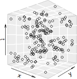
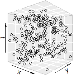
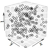
Figure 1: Realizations of Model 1 (left); Model 2 (middle); Model 3 (right).

According to [3], we generate a spatio-temporal Poisson process with intensity $\rho=4n(\textbf{x})$ (resp. $4n(\textbf{x})/\ell(W)$) as dummy points in Algorithm 1 (resp. Algorithm 2). For each model, we compute the root mean square error (RMSE) of each set of estimated parameters (Table 2) and plot the related boxplots (Figure 2). In Table 2 the lowest RMSE value is in bold and in Figure 2 the true values are represented by horizontal red lines. Both RMSE and boxplots show that the logistic likelihood approach performs better than the pseudo-likelihood approach for any model.

Table 2: RMSE of parameter estimates from 100 simulated realizations of the multi-scale Geyer point process model.

	Model 1			Model 2			Model 3
Method	$\hat{\lambda}$	$\hat{\gamma}_{1}$	$\hat{\gamma}_{2}$	$\hat{\lambda}$	$\hat{\gamma}_{1}$	$\hat{\gamma}_{2}$	$\hat{\lambda}$	$\hat{\gamma}_{1}$	$\hat{\gamma}_{2}$
pseudo	62.09	0.59	0.25	103.74	0.09	0.27	22.13	0.45	0.29
logistic	12.07	0.18	0.16	17.30	0.08	0.08	27.48	0.20	0.12

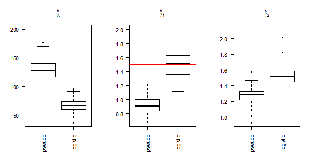
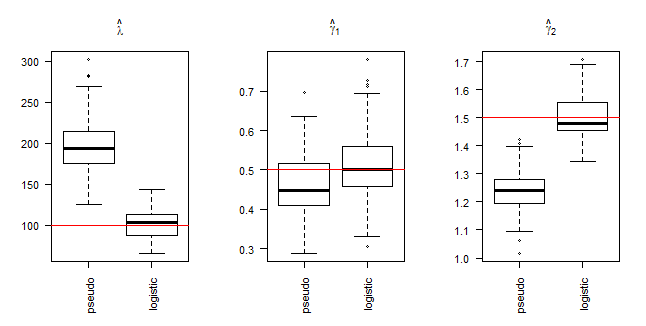
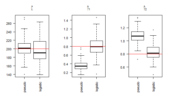
Figure 2: Boxplots of regular parameters estimated from the pseudo-likelihood and logistic likelihood approaches for Model 1 (first row), Model 2 (second row) and Model 3 (third row). True values are represented by horizontal red lines.

Note that in the spatial framework, [3] showed that for large datasets the logistic likelihood method is preferable than the pseudo-likelihood method as it requires a smaller number of dummy points and performs quickly and efficiently.  [18] and [15] investigated a similar comparison when these methods are regularized (i.e. using an approach with a simultaneous parameter estimation and variable selection by maximizing a penalized likelihood functions).  [29] found the advantage of the logistic likelihood approach for the spatio-temporal multi-scale area-interaction point process model. We here confirm this advantage for the spatio-temporal multi-scale Geyer point process model.

5 Application to forest fire occurrences

Economic and ecological disasters caused by wildfires in the world have led the scientific community to develop many novel statistical analysis and modelling wildfire occurrences to better understand their behaviors. In this section, we focus on the modelling of forest fire occurrences in the Bouches-du-Rhône county (Southern France) between 2001 and 2015.

Several statistical studies have shown the influence of environmental and meteorological factors on forest fire occurrences. In the French Mediterranean basin, [45] fit a spatio-temporal log-Gaussian Cox process model for forest fire occurrences with a log-linear intensity depending on spatio-temporal land use and weather covariates. [25] investigated the impact of the different covariates on the number of fires using multivariate analysis and [23] explored the influence of land cover covariates, temperature and precipitation on the probability of event occurrence. In addition to the spatio-temporal clustering of events induced by some covariates, [23] detected spatio-temporal interaction structures at different scales and notably an inhibitive effect that arises locally in time and space after wildfires as we expect lesser occurrences at these locations during a vegetation regeneration period.

We propose to fit the spatio-temporal hybrid Geyer point process model (5) on wildfire occurrences to take into account both the inhomogeneities induced by covariates and the multi-scale structure of interactions.

5.1 Data

Our data set is of the form $(\xi_{i},t_{i})$, $i=1,\dots,434$, where $(\xi_{i},t_{i})$ corresponds to a wildfire with more than $1$ hectare of burnt surface spatially indexed by a DFCI cell center $\xi_{i}$ in the Lambert 93 projection system and year $t_{i}\in\{2001,\dots,2015\}$. To avoid duplicated points we uniformly jittered $\xi_{i}$ in its DFCI cell. We refer the reader to [23] and [45] for further information on the data. Whilst forest fires are daily reported, we consider here the yearly scale, as done in many works (see e.g. [54, 52, 53]), because of the small number of reports and to optimize computation time in model fitting and validation steps. Figure 3 plots locations of forest fires (left panel) and yearly number of occurrences (right panel). It shows some clustering at short and medium spatial distances. Note that there exist two particular areas without any fire occurrences as they correspond to a lake (center) and marshlands (South-West). The number of fires slightly exponentially decreases in time over the 15 years, mainly due to improvements of fire-fighting resources.

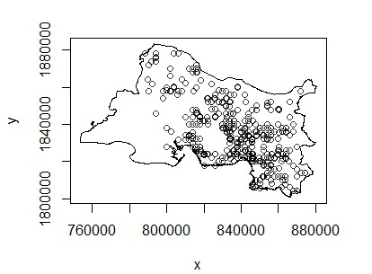
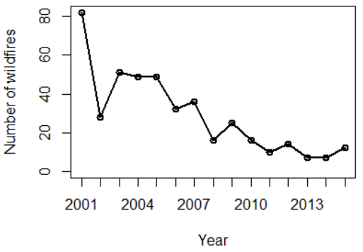
Figure 3: (Left) Forest fire locations in UTM coordinate system (distance in meters), with more than 1 hectare of burnt area, recorded during the years $2001$ to $2015$ in the Bouches-du-Rhône county in France. (Right) Number of recorded forest fires per year.

We consider the same framework as in [23] and restrict our attention to the following covariates: water coverage, elevation, coniferous cover and building cover as spatial covariates and temperature average, precipitation as spatio-temporal covariates. Hence, we can consider these covariates as good proxies of the main environmental, climatic and human factors. Maps of covariates are shown in Figure 4 in 2001.

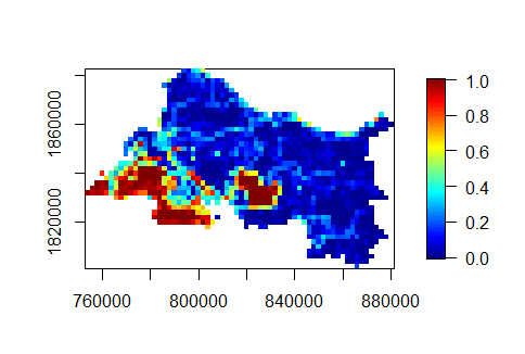
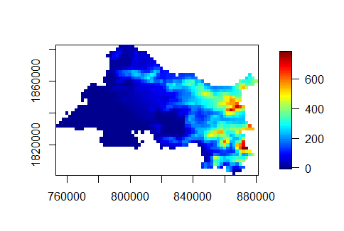
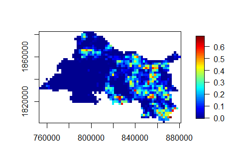
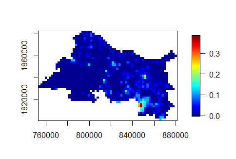
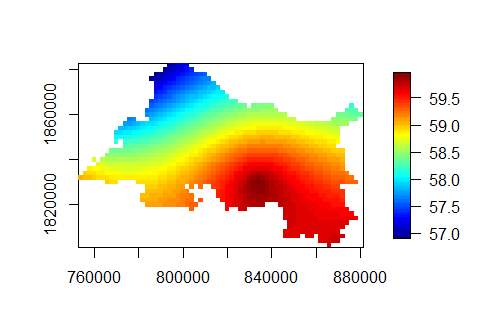
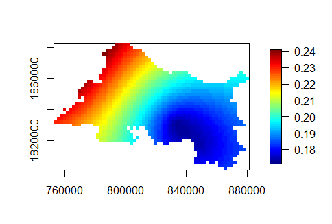
Figure 4: Maps of covariates: water coverage (top left), elevation (top right), coniferous cover (middle left), building cover (middle right), temperature average (botton left) and square root of precipitation (botton right) in 2001.

5.2 Model fitting

Here we first estimate the spatio-temporal trend and then fit the multi-scale spatio-temporal Geyer model to forest fire occurrences.

5.2.1 Spatio-temporal trend estimation

We express the spatio-temporal trend (5) as $\lambda(\xi,t)=\beta\mu(\xi,t)$ where $\log\mu(\xi,t)$ is assumed to linearly depend on covariates:

$$\log\mu(\xi,t)=\beta_{0}+\sum_{k=1}^{4}\beta_{k}^{S}Z_{k}^{S}(\xi)+\sum_{l=1}^{2}\beta_{l}^{ST}Z_{l}^{ST}(\xi,t)+\alpha t$$ (22)

with $Z_{k}^{S}(\xi)$, $k=1,\dots,4$, the spatial covariates, $Z_{l}^{ST}(\xi,t)$, $l=1,2$, the spatio-temporal covariates and $\alpha t$ a decreasing trend of fire counts over time. the coefficient $\beta$ will be estimated simultaneously with the others regular parameters by the logistic likelihood approach. Table 3 reports the coefficients $\beta_{0}$, $\beta_{k}^{S}$, $\beta_{l}^{ST}$ and $\alpha$ estimated as in [23] and [45]. The sign indicates if covariates favour (if positive, like coniferous, building and temperature) or prevent (if negative, like water, elevation, precipitation and time) fire occurrences. All covariates are significant and results are consistent with previous works.

Table 3: Estimated coefficients, standard errors and $p$-values based on two-tailed Student’s t-tests of significant differences from zero.

Covariates	Coefficients	Estimates	Standard error	$p$-value
Intercept	$\beta_{0}$	262	26	$<2\times 10^{-16\hskip 2.84526pt***}$
Water	$\beta_{1}^{S}$	-1.88	0.29	5.89$\times 10^{-11\hskip 2.84526pt***}$
Elevation	$\beta_{2}^{S}$	-0.001	0.0004	$0.0008^{\hskip 2.84526pt***}$
Coniferous	$\beta_{3}^{S}$	0.77	0.36	$0.031^{\hskip 2.84526pt*}$
Building	$\beta_{4}^{S}$	4	0.89	8.08$\times 10^{-6\hskip 2.84526pt***}$
Temperature	$\beta_{1}^{ST}$	0.37	0.06	1.13$\times 10^{-10\hskip 2.84526pt***}$
Precipitation	$\beta_{2}^{ST}$	-11.3	1.48	$1.75\times 10^{-14\hskip 2.84526pt***}$
Time	$\alpha$	-0.14	0.001	$<2\times 10^{-16\hskip 2.84526pt***}$

5.2.2 Parameters estimation

There is no common method for estimating irregular parameters in spatial or spatio-temporal Gibbs point process models. Here we considered several combinations of ad-hoc values within a reasonable range and select the optimal irregular parameters according to the Akaike’s Information Criterion (AIC) of the fitted model.

[6] suggest that the spatial interaction radius $r$ of the Geyer saturation point process should be between 0 and the maximum nearest neighbor distance, about 8000 meters for our dataset. For the temporal radius $q$, we consider small values to be in accordance with the natural phenomena of forest fire occurrences. Finally, for the saturation parameter $s$, we have $n(C_{r}^{q}(\xi_{i},t_{i});\textbf{x})\leq s$ for all $(\xi_{i},t_{i})\in\textbf{x}$. Hence, for any pair $(r,q)$, we set $s=\max_{1\leq i\leq n}n(C_{r}^{q}(\xi_{i},t_{i});\textbf{x})$.

According to the former section, we use the logistic likelihood method and Algorithm 2 to estimate the regular parameters. We simulate dummy points from an inhomogeneous Poisson point process with intensity $\rho(\xi,t)=C\mu(\xi,t)/\nu$ where $C=4$ by a classical rule of thumb in the logistic likelihood approach and $\nu=2000\times 2000\times 1$ (area of a DFCI cell multiplied by 1 year).

We fitted the spatio-temporal multi-scale Geyer point process model for a range of ad-hoc values $(r_{j},q_{j})\in[0,8000]\times\{1,2,3,4,5\}$, and their corresponding values of $s_{j}$, $j=1,\dots,m$, with varying $m$ in $\{1,2,3,4,5\}$. The minimum AIC is obtained for the combination given in Table 4. Estimated regular parameters show a strong clustering at short distances, randomness at medium and large distances and weak evidence of inhibition.

Table 4: Parameter estimates for $m=4$.

Irregular parameters
$r$	500	2000	5000	7500
$q$	1	2	3	4
$s$	4	7	27	57
Regular parameters
$\hat{\beta}=0.66$	$\hat{\gamma}_{1}=2.73$,	$\hat{\gamma}_{2}=0.93$	$\hat{\gamma}_{3}=1.07$	$\hat{\gamma}_{4}=0.98$

5.3 Model validation

We validate our fitted model from Monte Carlo tests using statistics based on the spatio-temporal inhomogeneous $K$-function [22]. First, we generate $n_{sim}=99$ simulations from our fitted hybrid Geyer model (5) by Algorithm 3 with a burn-in period of $70,000$ steps, representing realizations from our null hypothesis. Then, we compute the spatio-temporal inhomogeneous $K$-function for the observed and simulated point patterns, denoted respectively by $\hat{K}_{obs}^{inh}(h_{s},h_{t})$ and $\hat{K}_{i}^{inh}(h_{s},h_{t}),i\in\{1,...,n_{sim}\}$, with an estimated non-separable intensity function obtained by kernel smoothing. For each value of the spatio-temporal distance $(h_{s},h_{t})$, lower ($L$) and upper ($U$) critical envelopes of the summary statistics are computed

$$L(h_{s},h_{t})=\min_{1\leq i\leq n_{sim}}\hat{K}_{i}^{inh}(h_{s},h_{t}),\quad U(h_{s},h_{t})=\max_{1\leq i\leq n_{sim}}\hat{K}_{i}^{inh}(h_{s},h_{t}).$$ (23)

In addition to these local envelopes, we compute local and global $p$-values as in [59, 55] in order to respectively detect spatio-temporal distances where the departure from the null hypothesis is the most significant and the overall adequacy of our model. Let $E(h_{s},h_{t})$ and $V(h_{s},h_{t})$ denote the mean and variance of $\left\{\hat{K}_{1}^{inh}(h_{s},h_{t}),\dots,\hat{K}_{n_{sim}}^{inh}(h_{s},h_{t}),\hat{K}_{obs}^{inh}(h_{s},h_{t})\right\}$. We define the local $p$-value for each pair $(h_{s},h_{t})$ by

$$p(h_{s},h_{t})=\frac{1+\sum_{i=1}^{n_{sim}}\mathbbm{1}\{T_{i}(h_{s},h_{t})>T_{obs}(h_{s},h_{t})\}}{n_{sim}+1},$$ (24)

where $T_{i}(h_{s},h_{t})$ (resp. $T_{obs}(h_{s},h_{t})$) denotes the local statistic $T$ computed from the $i^{th}$ simulation (resp. the data) at $(h_{s},h_{t})$. The local statistic is defined by

$$T(h_{s},h_{t})=\sqrt{\frac{(\hat{K}^{inh}(h_{s},h_{t})-E(h_{s},h_{t}))^{2}}{V(h_{s},h_{t})}}.$$ (25)

The global test combines the information for all spatial and temporal distances. We define the test statistic

$$\tilde{T}=\int_{0}^{h_{t,max}}\int_{0}^{h_{s,max}}T(h_{s},h_{t})dh_{s}dh_{t},$$ (26)

where $h_{s,max}$ and $h_{t,max}$ are user-specific maximum spatial and temporal distances which are preferable to choose close to the (expected) range of interaction of the underlying point process. [31] recommends to compare the results for several values of $h_{s,max}$ and $h_{t,max}$. The $p$-value of the global test is then given by

$$p_{global}=\frac{1+\sum_{i=1}^{n_{sim}}\mathbbm{1}\{\tilde{T}_{i}>\tilde{T}_{obs}\}}{n_{sim}+1}.$$

Figure 5.$a)$ shows the spatio-temporal inhomogeneous $K$ function computed on our dataset (dark grey) and the envelopes obtained from our hybrid Geyer model (light grey); $\hat{K}_{obs}^{inh}(h_{s},h_{t})$ lies inside the envelopes, meaning that the fitted model seems to describe properly the spatio-temporal structure of the data. This is confirmed by local $p$-values at any distances (Figure 5.$b)$. Global $p$-values are given in Figure 5.$c)$ for any combination of $h_{s,max}$ and $h_{t,max}$. Again, it shows that our fitted model is validated.

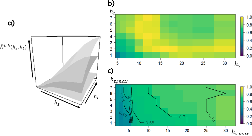
Figure 5: Temporal separations $h_{t}$ are in year and spatial distances $h_{s}$ are in kilometer. $a)$ Envelopes of the spatio-temporal inhomogeneous $K$-function for the simulated spatio-temporal multi-scale Geyer point process according to the estimated parameters. $b)$ Image plot of the local $p$-value. $c)$ Image plot of the global $p$-value for any pairs of $(h_{s,max},h_{t,max})$.

Note that we did the same tests for 99 simulations of an inhomogeneous Poisson process with intensity $\mu(\xi,t)/(2000\times 2000\times 1)$ (22). This model has been rejected at the level $5\%$, with a median global $p$-value equals to 0.04.

Conclusion

Due to the capability of Gibbs point processes to cover prevalent structures (inhibition, randomness and clustering), the hybridization approach allows to introduce new Gibbs models combining several structures at different scales. In this paper, we defined the spatio-temporal multi-scale Geyer saturation point process model and detailed the classical statistical inference methods and MCMC simulation techniques that we have extended to the spatio-temporal framework and implemented in R code that will be added to the stpp package [24]. Our simulation study highlighted a better goodness-of-fit of parameters for the logistic likelihood approach compared to the pseudo-likelihood approach. Finally, we illustrated the interest of using this model on a spatio-temporal dataset of forest fire locations associated with environment covariates. The model validation shows that our model captures the multi-scale interaction structure inherent to forest fire occurrences.

In this paper, we focused our attention on the definition of a new hybrid Gibbs model, the inference methods and MCMC simulation algorithms that we needed to adapt to the spatio-temporal context. Some of our choices can be discussed and eventually improved in future works, notably in our application to forest fire occurrences which is not presented as an in-depth study but as an illustration of the model fitting on real data.

In our application study, we considered a log-linear form for the trend depending on covariate information. We chose a two-step procedure for estimating, at first, the trend coefficients and then the regular parameters of the interaction function. Our knowledge on forest fire mechanisms guided this choice because the main driver of occurrence locations is the environmental heterogeneity and the secondary one is the interaction phenomena. The trend is estimated at the spatial DFCI scale and at the yearly one, corresponding to our covariate resolution. In that way, we estimated a global trend at a medium scale whereas the interaction parameters are estimated at the point locations and represent a local interaction behavior at a fine scale. This procedure could be improved by incorporating variable selection methods, e.g. via regularization [15, 18].

Our two-step estimation procedure allows us to provide confidence intervals for the trend coefficients but we have not explored the significance testing of the regular parameters in the interaction function. We notice that some parameters $\gamma_{j}$ are closed to one and testing departure from one is possible by extending the adjusted composite likelihood ratio test [8] to the spatio-temporal framework or by considering parametric bootstrap procedures. Here, we decided to present the testing of the overall goodness-of-fit of our model instead of focusing our work on the pointwise significance of the interaction parameters.

For the choice of irregular parameters, because the likelihood is not differentiable with respect to them, we used a maximum profile likelihood approach based on the logistic likelihood estimation procedure and AIC values for model selection. Introduced for the pseudo-likelihood estimates in [1] and applied to the logistic likelihood approach by us using the results in [3], this method consists in fixing irregular parameters and maximizing the composite likelihood with respect to the regular ones. This technique is a computationally-intensive method. Thanks to a preliminary spatio-temporal exploratory analysis of the interaction ranges done with the inhomogeneous pair correlation function $g$, the maximum nearest neighbor distance and the temporal autocorrelation function, we chose few configurations of feasible values for the nuisance parameters $m$, $r_{j}$, $q_{j}$ and $s_{j}$, $j=1\dots m$. Considering more values would be very time-consuming and developing a new estimation method would be a subject in its own right.

Our model can be used in many fields, like seismology and epidemiology for example, because several mechanisms exhibit interaction between points at multiple scales in space and time. Relying on this work, we can also develop hybrid models with different density structures. Indeed, although it was not necessarily highlighted here, we know that forest fires with large burnt areas avoid future fire occurrences during a vegetation regeneration period. Such cases of strong inhibition may be modeled by hybrid Gibbs point processes with a hardcore component like the hybrid Geyer hardcore point process. We recently extended our work to this model.

References

- Anwar and Stein [2015] Anwar, S., Stein, A., 2015. Spatial pattern development of selective logging over several years. Spatial Statistics 13, 90–105. doi:10.1016/j.spasta.2015.03.001.
- Arago et al. [2016] Arago, P., Juan, P., Diaz-Avalos, C., Salvador, P., 2016. Spatial point process modeling applied to the assessment of risk factors associated with forest wildfires incidence in Castellon, Spain. European Journal of Forest Research 135, 451–464. doi:10.1007/s10342-016-0945-z.
- Baddeley et al. [2014] Baddeley, A., Coeurjolly, J., Rubak, E., Waagepetersen, R., 2014. Logistic regression for spatial Gibbs point processes. Biometrika 101, 377–392. doi:10.1093/biomet/ast060.
- Baddeley et al. [2019] Baddeley, A., Rubak, E., Turner, R., 2019. Leverage and influence diagnostics for Gibbs spatial point processes. Spatial Statistics 29, 15–48. doi:10.1016/j.spasta.2018.09.004.
- Baddeley and Turner [2000] Baddeley, A., Turner, R., 2000. Practical maximum pseudolikelihood for spatial point patterns (with discussion). Australian and New Zealand Journal of Statistics 42, 283–322. doi:10.1111/1467-842X.00128.
- Baddeley and Turner [2006] Baddeley, A., Turner, R., 2006. Modelling spatial point patterns in R, in: Baddeley, A., Gregori, P., Mateu, J., Stoica, R., Stoyan, D. (Eds.), Case Studies in Spatial Point Process Modeling. Lecture Notes in Statistics. Springer, New York. volume 185, pp. 23–74. doi:10.1007/0-387-31144-0_2.
- Baddeley et al. [2013] Baddeley, A., Turner, R., Mateu, J., Bevan, A., 2013. Hybrids of Gibbs point process models and their implementation. Journal of Statistical Software 55, 1–43. doi:10.18637/jss.v055.i11.
- Baddeley et al. [2016] Baddeley, A., Turner, R., Rubak, E., 2016. Adjusted composite likelihood ratio test for spatial Gibbs point processes. Journal of Statistical Computation and Simulation 86, 922–941. doi:10.1080/00949655.2015.1044530.
- Berman and Turner [1992] Berman, M., Turner, R., 1992. Approximating point process likelihoods with GLIM. Applied Statistics 41, 31–38. doi:10.1016/0167-6687(93)90845-G.
- Besag [1977] Besag, J., 1977. Some methods of statistical analysis for spatial data. Bulletin of the International Statistical Institute 47, 77–92.
- Brix and Chadœuf [2000] Brix, A., Chadœuf, J., 2000. Spatio-temporal modeling of weeds and shot-noise G Cox processes. Biometrical Journal 44, 83–99. doi:10.1002/1521-4036(200201)44:1<83::AID-BIMJ83>3.0.CO;2-W.
- Brix and Diggle [2001] Brix, A., Diggle, P., 2001. Spatiotemporal prediction for log-Gaussian Cox processes. Journal of the Royal Statistical Society. Series B (Statistical Methodology) 63, 823–841. doi:10.1111/1467-9868.00315.
- Brix and Kendal [2002] Brix, A., Kendal, W., 2002. Simulation of cluster point processes without edge effects. Advances in Applied Probability 34, 267–280. doi:10.1239/aap/1025131217.
- Brix and Møller [2001] Brix, A., Møller, J., 2001. Space-time multitype log Gaussian Cox processes with a view to modelling weed data. Journal Scandinavian Journal of Statistics 28, 471–488. doi:10.1111/1467-9469.00249.
- Choiruddin et al. [2018] Choiruddin, A., Coeurjolly, J., Letué, F., 2018. Convex and non-convex regularization methods for spatial point processes intensity estimation. Electronic Journal of Statistics 12, 1210–1255. doi:10.1214/18-EJS1408.
- Cox [1972] Cox, D., 1972. The statistical analysis of dependencies in point processes, in: Lewis, P. (Ed.), Stochastic Point Processes. Wiley, New York, pp. 55–66.
- Cronie and van Lieshout [2015] Cronie, O., van Lieshout, M., 2015. A J-function for inhomogeneous spatio-temporal point processes. Scandinavian Journal of Statistics 42, 562–579. doi:10.1111/sjos.12123.
- Daniel et al. [2018] Daniel, J., Horrocks, J., Umphrey, G., 2018. Penalized composite likelihoods for inhomogeneous Gibbs point process models. Computational Statistics and Data Analysis 124, 104–116. doi:10.1016/j.csda.2018.02.005.
- Dereudre [2019] Dereudre, D., 2019. Introduction to the theory of Gibbs point processes, in: Coupier, D. (Ed.), Stochastic Geometry. Springer, pp. 181–229. doi:10.1007/978-3-030-13547-8_5.
- Diggle et al. [2013] Diggle, P., Moraga, P., Rowlingson, B., Taylor, B., 2013. Spatial and spatio-temporal log-Gaussian Cox processes: extending the geostatistical paradigm. Statistical Science 28, 542–563. doi:10.1214/13-STS441.
- Gabriel [2014] Gabriel, E., 2014. Estimating second-order characteristics of inhomogeneous spatio-temporal point processes. Methodology and Computing in Applied Probability 16, 411–431. doi:10.1007/s11009-013-9358-3.
- Gabriel and Diggle [2009] Gabriel, E., Diggle, P., 2009. Second-order analysis of inhomogeneous spatio-temporal point process data. Statistica Neerlandica 63, 43–51. doi:10.1111/j.1467-9574.2008.00407.x.
- Gabriel et al. [2017] Gabriel, E., Opitz, T., Bonneu, F., 2017. Detecting and modeling multi-scale space-time structures: the case of wildfire occurrences. Journal of the French Statistical Society 158, 86–105.
- Gabriel et al. [2013] Gabriel, E., Rowlingson, B., Diggle, P., 2013. stpp: a R package for plotting, simulating and analyzing spatio-temporal point patterns. Journal of Statistical Software 53, 1–29. doi:10.18637/jss.v053.i02.
- Ganteaume and Jappiot [2013] Ganteaume, A., Jappiot, M., 2013. What causes large fires in Southern France. Forest Ecology and Management 294, 76–85. doi:10.1016/j.foreco.2012.06.055.
- Geyer [1999] Geyer, C., 1999. Likelihood inference for spatial point processes, in: Barndorff-Nielsen, O., Kendall, W., van Lieshout, M. (Eds.), Stochastic Geometry: Likelihood and Computation. Chapman and Hall, London. volume 80, pp. 79–140. doi:10.1201/9780203738276-3.
- Geyer and Møller [1994] Geyer, C., Møller, J., 1994. Simulation procedures and likelihood inference for spatial point processes. Scandinavian Journal of Statistics 18, 505–544.
- Gonzalez et al. [2016] Gonzalez, J., Rodriguez-Cortes, F., Cronie, O., Mateu, J., 2016. Spatio-temporal point process statistics: A review. Spatial Statistics 18, 505–544. doi:10.1016/j.spasta.2016.10.002.
- Iftimi et al. [2018] Iftimi, A., van Lieshout, M., Montes, F., 2018. A multi-scale area-interaction model for spatio-temporal point patterns. Spatial Statistics 26, 38–55. doi:10.1016/j.spasta.2018.06.001.
- Iftimi et al. [2017] Iftimi, A., Montes, F., Mateu, J., Ayyad, C., 2017. Measuring spatial inhomogeneity at different spatial scales using hybrids of Gibbs point process models. Stochastic Environmental Research and Risk Assessment 31, 1455–1469. doi:10.1007/s00477-016-1264-0.
- Illian et al. [(2008] Illian, J., Penttinen, A., Stoyan, H., Stoyan, D., (2008). Statistical Analysis and Modelling of Spatial Point Patterns. John Wiley & Sons, Chichester. doi:10.1002/9780470725160.
- Juan et al. [2012] Juan, P., Mateu, J., Saez, M., 2012. Pinpointing spatio-temporal interactions in wildfire patterns. Stochastic Environmental Research and Risk Assessment 26, 1131–1150. doi:10.1007/s00477-012-0568-y.
- Kingman [1993] Kingman, J., 1993. Poisson Processes. volume 3. Oxford University Press, Oxford.
- Kingman [2006] Kingman, J., 2006. Poisson processes revisited. Probability and Mathematical Statistics 26, 77–95.
- Lavancier et al. [2015] Lavancier, F., Møller, J., Rubak, E., 2015. Determinantal point process models and statistical inference. Journal of the Royal Statistical Society. Series B (Statistical Methodology) 77, 853–877. doi:10.1111/rssb.12096.
- Levin [1992] Levin, C., 1992. The problem of pattern and scale in ecology: The Robert H. Macarthur award lecture. Ecology 73, 1943–1967. doi:10.2307/1941447.
- Macchi [1975] Macchi, O., 1975. The coincidence approach to stochastic point processes. Advances in Applied Probability 7, 83–122. doi:10.2307/1425855.
- Matérn [(1960] Matérn, B., (1960). Spatial Variation. Lectures Notes in Statistics. Springer-Verlag, Chichester. doi:10.1007/978-1-4615-7892-5.
- Møller and Diaz-Avalos [2010] Møller, J., Diaz-Avalos, C., 2010. Structured spatio-temporal shot-noise Cox point process models, with a view to modelling forest fires. Scandinavian Journal of Statistics 37, 2–25. doi:10.1111/j.1467-9469.2009.00670.x.
- Møller et al. [1998] Møller, J., Syversveen, A., Waagepetersen, R., 1998. Log Gaussian Cox processes. Scandinavian Journal of Statistics 25, 451–482. doi:10.1111/1467-9469.00115.
- Møller and Waagepetersen [(2004] Møller, J., Waagepetersen, R., (2004). Statistical Inference and Simulation for Spatial Point Processes. Chapman and Hall/CRC, Boca Raton. doi:10.1201/9780203496930.
- Neyman and Scott [1958] Neyman, J., Scott, E., 1958. Statistical approach to problems of cosmology. Journal of the Royal Statistical Society. Series B (Methodological) 20, 1–29. doi:10.1111/j.2517-6161.1958.tb00272.x.
- Ogata and Tanemura [1981] Ogata, Y., Tanemura, M., 1981. Estimation of interaction potentials of spatial point patterns through the maximum likelihood procedure. Annals of the Institute of Statistical Mathematics 33, 315–338. doi:10.1007/BF02480944.
- Opitz [2009] Opitz, T., 2009. Simulating and fitting of Gibbs processes in 3D–models, algorithms and their implementation. Master’s thesis. Ulm University. Germany.
- Opitz et al. [2020] Opitz, T., Bonneu, F., Gabriel, E., 2020. Point-process based Bayesian modeling of space-time structures of forest fire occurrences in Mediterranean France. Spatial Statistics , 100429.doi:10.1016/j.spasta.2020.100429.
- Papangelou [1974] Papangelou, F., 1974. The conditional intensity of general point processes and an application to line processes. Probability Theory and Related Fields 28, 207–226. doi:10.1007/BF00533242.
- Picard et al. [2009] Picard, N., Bar-Hen, A., Mortier, F., Chadoeuf, J., 2009. The multi-scale marked area-interaction point process: a model for the spatial pattern of trees. Scandinavian Journal of Statistics 36, 23–41. doi:10.1111/j.1467-9469.2008.00612.x.
- R Core Team [2016] R Core Team, 2016. R: A Language and Environment for Statistical Computing. R Foundation for Statistical Computing. URL: https://www.R-project.org.
- Raeisi et al. [2019] Raeisi, M., Bonneu, F., Gabriel, E., 2019. On spatial and spatio-temporal multi-structure point process models. Les Annales de l’ISUP 63.
- Ripley and Kelly [1977] Ripley, B., Kelly, F., 1977. Markov point processes. Journal of the London Mathematical Society 15, 188–192. doi:10.1112/jlms/s2-15.1.188.
- Serra et al. [2013] Serra, L., Juan, P., Varga, D., Mateu, J., Saez, M., 2013. Spatial pattern modelling of wildfires in Catalonia, Spain 2004–2008. Environmental Modelling and Software 40, 235–244. doi:10.1016/j.envsoft.2012.09.014.
- Serra et al. [2014a] Serra, L., Saez, M., Juan, P., Varga, D., Mateu, J., 2014a. A spatio-temporal Poisson hurdle point process to model forest fires. Stochastic Environmental Research and Risk Assessment 28, 1671–1684. doi:10.1007/s00477-013-0823-x.
- Serra et al. [2014b] Serra, L., Saez, M., Mateu, J., Varga, D., Juan, P., Diaz-Avalos, C., 2014b. Spatio-temporal log-Gaussian Cox processes for modelling wildfire occurrence: the case of Catalonia, 1994–2008. Environmental and Ecological Statistics 21, 531–563. doi:10.1007/s10651-013-0267-y.
- Serra et al. [2012] Serra, L., Saez, M., Varga, D., Tobias, A., Mateu, J., 2012. Spatio-temporal modelling of wildfires in Catalonia, Spain, 1994–2008, through log Gaussian Cox processes. WIT Transactions on Ecology and the Environment 158, 34–49. doi:10.2495/FIVA120041.
- Siino et al. [2018a] Siino, M., Adelfio, G., Mateu, J., 2018a. Joint second-order parameter estimation for spatio-temporal log-Gaussian Cox processes. Stochastic Environmental Research and Risk Assessment 32, 3525–3539. doi:10.1007/s00477-018-1579-0.
- Siino et al. [2017] Siino, M., Adelfio, G., Mateu, J., Chiodi, M., D’Alessandro, A., 2017. Spatial pattern analysis using hybrid models: an application to the Hellenic seismicity. Stochastic Environmental Research and Risk Assessment 31, 1633–1648. doi:10.1007/s00477-016-1294-7.
- Siino et al. [2018b] Siino, M., D’Alessandro, A., Adelfio, G., Scudero, S., Chiodi, M., 2018b. Multiscale processes to describe the eastern sicily seismic sequences. Annals of Geophysics 61, 1–17. doi:10.4401/ag-7688.
- Strauss [1975] Strauss, D., 1975. A model for clustering. Biometrika 62, 467–475. doi:10.1093/biomet/62.2.467.
- Tamayo-Uria et al. [2014] Tamayo-Uria, I., Mateu, J., Diggle, P., 2014. Modelling of the spatiotemporal distribution of rat sightings in an urban environment. Spatial Statistics 9, 192–206. doi:10.1016/j.spasta.2014.03.005.
- Trilles et al. [2013] Trilles, S., Juan, P., Diaz, L., Arago, P., Huerta, J., 2013. Integration of environmental models in spatial data infrastructures: a use case in wildfire risk prediction. IEEE Journal of Selected Topics in Applied Earth Observations and Remote Sensing 6, 128–138. doi:10.1109/JSTARS.2012.2236538.
- Turner [2009] Turner, R., 2009. Point patterns of forest fire locations. Environmental and Ecological Statistics 16, 197–223. doi:10.1007/s10651-007-0085-1.
- Wiegand et al. [2007] Wiegand, T., Gunatillekem, N., Okudam, T., 2007. Analyzing the spatial structure of a Sri Lankan tree species with multiple scales of clustering. Ecology 88, 3088–3102. doi:10.1890/06-1350.1.
- Woo et al. [2017] Woo, H., Chung, W., Graham, J., Lee, B., 2017. Forest fire risk assessment using point process modelling of fire occurrence and Monte Carlo fire simulation. International Journal Wildland Fire 26, 789–805. doi:10.1071/WF17021.