Long Range 3D with Quadocular Thermal (LWIR) Camera

Abstract

Long Wave Infrared (LWIR) cameras provide images regardless of the ambient illumination, they tolerate fog and are not blinded by the incoming car headlights. These features make LWIR cameras attractive for autonomous navigation, security and military applications. Thermal images can be used similarly to the visible range ones, including 3D scene reconstruction with two or more such cameras mounted on a rigid frame. There are two additional challenges for this spectral range: lower image resolution and lower contrast of the textures.

In this work, we demonstrate quadocular LWIR camera setup, calibration, image capturing and processing that result in long range 3D perception with 0.077 pix disparity error over 90% of the depth map. With low resolution ($160\times 120$) LWIR sensors we achieved 10% range accuracy at 28 m with $56^{\circ}$ horizontal field of view (HFoV) and 150 mm baseline. Scaled to the now-standard $640\times 512$ resolution and 200 mm baseline suitable for head-mounted application the result would be 10% accuracy at 130 m.

1. Introduction

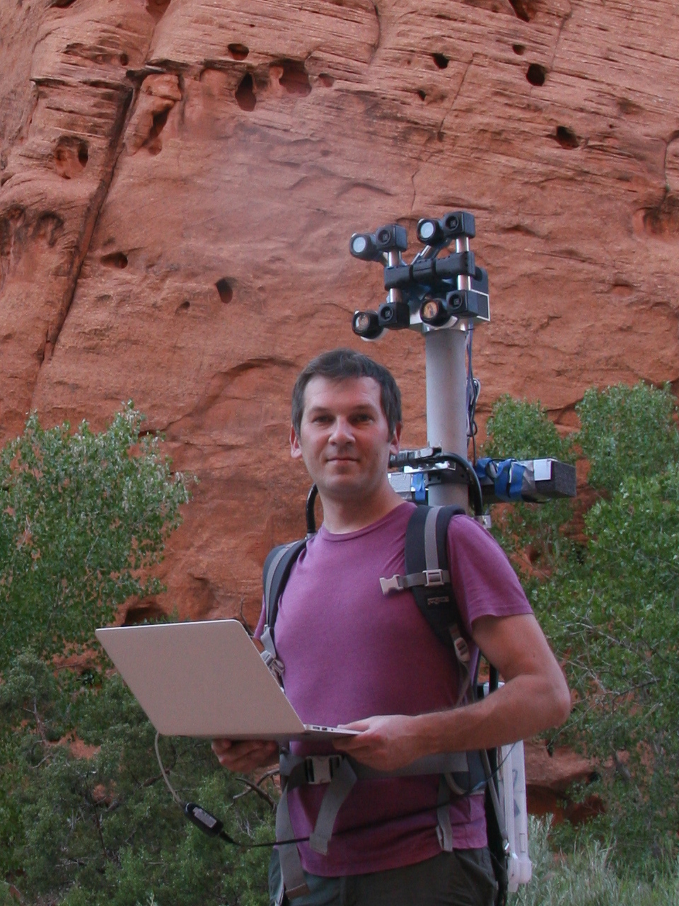
Figure 1: Dual quadocular LWIR +RGB experimental camera.

Advances in uncooled LWIR detectors based on microbolometer arrays made thermal imaging (TI) practical in multiple application areas where remote object’s temperature is important itself or where the temperature gradients and differences can be used for localization, object detection, and tracking, 3D scene reconstruction. Temperature measurements combined with 3D data are needed in medical applications (Chernov et al. [6], Cao et al. [4]), energy auditing (Vidas and Moghadam [32], [4]). High thermal contrast of live objects facilitates foreground (FG)/background (BG) separation in 3D models for counting pedestrians (Kristoffersen et al. [17]). The main application of the TI fused with the other data sources remains autonomous and assisted driving. While not considering specifically TI 3D, Miethig et al. [20] compare it with other sensors (LIDARs, radars, sonars, and RGB camera) arguing that the use of TI could have prevented some fatalities that were caused by autonomously driven cars. They mention high contrast for the living organisms in any weather conditions, resilience to fog, as well as the fact that LWIR sensors are not saturated by the headlights of the incoming traffic.

Most of the known 3D perception systems rely on multimodal data, such as RGB, TI, and depth. Treible et al. [30] created a 3-modal benchmark set, where synchronized binocular RGB and LWIR are combined with a ground truth image captured with a LIDAR. LWIR-only 3D perception is beneficial for the military applications where active ranging methods (LIDAR, time-of-flight (ToF) or structured light) are easily detectable by the properly equipped adversary. 3D perception for unmanned ground vehicle (UGV) was researched by Lee et al. [18], Zapf et al. [34], and while the experimental rig was tri-modal, they evaluated LWIR-only performance too while using LIDAR data as a ground truth.

We developed and evaluated a quadocular LWIR 3D perception system (Figure 1) that is paired with another RGB quadocular camera (Elphel MNC393-XCAM) as a source of the ground truth data for the DNN training and evaluation. LWIR system uses four $160\text{\times}120\text{\,}$ FLIR Lepton modules, the RGB cameras have $2592\text{\times}1936\text{\,}$ sensors with $16\times$ higher linear resolution. This ratio and almost identical values for the field of view (FoV), baseline, and mean reprojection error (MRE), measured in pixels for both modalities made it possible to consider the depth map generated from the RGB images as ground truth for the LWIR ones – for every matched object distance the expected range error for LWIR is 13 times larger than that of the RGB modality.

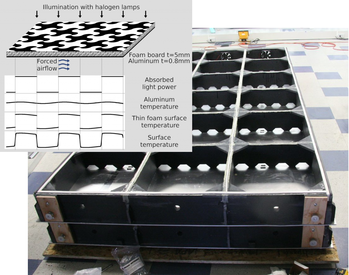
Figure 2: LWIR calibration pattern design and a rear view of the calibration panel.

Our contributions are as follows:

1. Development of a LWIR quadocular camera prototype for wearable and small UGV applications;

2. Development of the large format ($7\text{\times}3\text{\,}\mathrm{m}$) dual-modal calibration system for high resolution photogrammetric and radiometric applications;

3. Adaptation of the long range RGB image processing open source software (Filippov and Dzhimiev [11]) to LWIR, evaluation of the prototype system and comparing its performance to state of the art.

The rest of the paper is organized as follows. In Section 2 we overview existing methods of the LWIR cameras calibration and describe our contribution. In Section 3 we explain our system hardware, image sets acquisition, low-level preprocessing, and training of the DNN to improve depth map accuracy. Finally, in Section 4 we compare our results with the prior ones.

2. Calibration

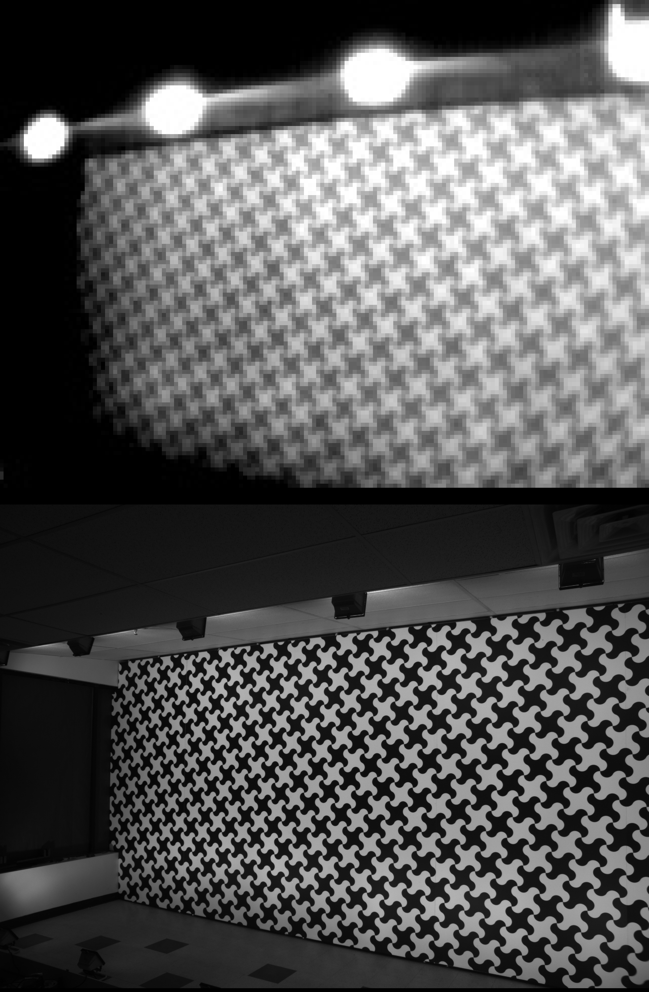
Figure 3: Calibration pattern views: LWIR (top), visible range (bottom).

2.1 Existing LWIR and Multimodal Calibration

Photogrammetric camera calibration is an important precondition to achieve an accurate depth map in the stereo application, and most methods use special calibration setups to perform this task. It is convenient to use a standard OpenCV calibration procedure, another popular (over 13,000 citations) approach was presented by Zhang [36], it is used by many TI and multimodal calibration systems. This method involves capturing an image of a checkerboard or a pattern of squares rotated at several angles (or moving the camera around), matching the corners of the squares and then using Levenberg-Marquardt algorithm (LMA) to simultaneously find camera extrinsic and intrinsic parameters by minimizing reprojection error. The challenge of the LWIR and multimodal calibrations is to make this pattern to be reliably registered by a thermal or all modalities.

Rangel et al. [23] provide a classification of the TI calibration for both active (heated by powered wires, resistors or LEDs) and passive (printed or cut pattern heated by a floodlight or sun) designs. They tested several targets and selected cardboard with the circular holes in front of a heated surface. Vidas et al. [31] used an A4-sized cardboard pattern with $20\text{\times}20\text{\,}\mathrm{mm}$ holes and a computer monitor as a heated BG, reporting no blurring of the corners. Skala et al. [27] used Styrofoam panel with cut square holes that worked well for both LWIR and depth sensors.

Just for the TI alone Ng et al. [21] suggested a heated wire net with plastic BG on a turntable, Prakash et al. [22] used printed checkerboard on paper with a flood lamp. Saponaro et al. [25] made the checkerboard corners sharper by attaching the paper pattern to a ceramic tile, they also measured the change of the target contrast over time after turning off the floodlight. LWIR image blur that makes matching points registration difficult was targeted by several other works. Harguess and Strange [14] made a pattern with $3\text{\times}5\text{\,}$ circles ($170\text{\,}\mathrm{mm}$ pitch) printed on $3\text{\,}\mathrm{mm}$ aluminum composite Dibond consisting of two $0.3\text{\,}\mathrm{mm}$ aluminum layers with the polyethylene core between them.

St-Laurent et al. [28] used a thermally conductive substrate – $2.4\text{\,}\mathrm{mm}$ solid aluminum instead of the aluminum laminate and achieved sharp LWIR images suitable for automatic corner detection with OpenCV and used it with tri-modal LWIR, Short Wave Infrared (SWIR), and visible range. Similar to the previous work this pattern required high irradiance power as the thermal difference was developed in the thin paint layer and was usable only outdoors under the bright sunlight. Rankin et al. [24] evaluated multiple calibration targets for LWIR and Middle Wave Infrared (MWIR), passive ones (heated by the sunlight) had $5\text{\times}5\text{\,}$ black dots printed on foamcore board attached to aluminum honeycomb, they also used heated plastic inserts on a metal frame and a large $1.3\text{\times}1.5\text{\,}\mathrm{m}$ checkerboard with heated wires along the edges developed by General Dynamics.

Other active methods depend on heated elements, such as light bulbs (Yang et al. [33], Zoetgnand et al. [37]), resistors (Gschwandtner et al. [13]) or overheated LEDs (Beauvisage and Aouf [2], Li et al. [19]).

Most of the referenced works report MRE in the range of few tenths of a pixel (0.41 pix [25], 0.2..0.8 pix [14], 0.1..0.2 pix [28], 0.22..0.25 pix [2], 0.36 pix [19], 0.3 pix,  [13], 0.25 pix [37]), but Ellmauthaler et al. [7] report much lower MRE or 0.036 pix and even 0.0287 pix in Ellmauthaler et al. [8]. While they are using an iterative process that calculates centers of mass of the rectified image of light bulbs instead of just coordinates of the corners, the reported MRE may be too optimistic because the target pattern image in each frame is too small. We would expect significantly higher MRE if the pattern was registered over the full frame.

Long range depth measurements require high disparity resolution, therefore, calibration has to provide low MRE over the full FoV. We achieve $\lx@glossaries@gls@link{main}{mre}{\leavevmode{\color[rgb]{0.23,0.27,0.29}{\color[rgb]{0.23,0.27,0.29}MRE}}}_{LWIR}=0.067~{}pix,\lx@glossaries@gls@link{main}{mre}{\leavevmode{\color[rgb]{0.23,0.27,0.29}{\color[rgb]{0.23,0.27,0.29}MRE}}}_{RGB}=0.036~{}pix$ by using a very large calibration pattern, bundle-adjusting the pattern nodes 3D coordinates simultaneously with calibrating of a multi-sensor high-resolution camera, and use of the accurate phase correlation matching of the registered patterns.

2.2 Dual-modality Calibration Target

Our dual-modality visible/LWIR $7.0\text{\times}3.0\text{\,}\mathrm{m}$ calibration target consists of five separate panels fitted together. The black-and-white pattern resembles the checkerboard one with each straight edge replaced by a combination of two arcs – such layout makes spatial spectrum uniform compared to a plain checkerboard pattern and facilitates point spread function (PSF) measurement of the cameras.

Figure 2 shows the construction and a back view of a $1.5\text{\times}3.0\text{\,}\mathrm{m}$ panel. This design provides a definite correspondence between the image registered by the visible range cameras and the surface temperature, resulting in time-invariant images for both modalities. The pattern illuminated by ten of $500\text{\,}\mathrm{W}$ halogen floodlights is printed on a $5\text{\,}\mathrm{mm}$ foamcore board glued to an $0.8\text{\,}\mathrm{mm}$ aluminum sheet. We found that it is important to use both inks – black and white because the unpainted paper surface of the white foamcore board behaves almost like a mirror showing flood light reflection in LWIR spectral range, while the paint bumps provide sufficient diffusion to mitigate this effect.

The pattern temperature does not depend much on uncontrolled convection as the back side of the pattern is cooled by the forced airflow. In our current experiments, we used the full power of the fans, but it is easy to control the airflow in each target segment and precisely maintain the temperature of the aluminum backing for radiometric calibration. High thermal conductance of the aluminum and low conductance of the foamcore board together with the small board thickness relative to the cell edge ($5\text{\,}\mathrm{mm}$ vs. $180\text{\,}\mathrm{mm}$) result in sharp and uniform LWIR images. For precise radiometric calibration, the residual non-uniformity and blur can be modeled to calculate the temperature from the light intensity registered by a visible range camera. Each target segment is made mechanically rigid by the structural elements cut from the thicker foamcore material. Additionally, when calibration is in progress, the fans provide negative air pressure holding the panels tightly against the wall.

During the calibration process several hundred image sets (4 RGB and 4 LWIR) are acquired using the robotic fixture, scanning $\pm 40\text{\,}\mathrm{\SIUnitSymbolDegree}$ horizontally and $\pm 25\text{\,}\mathrm{\SIUnitSymbolDegree}$ vertically with 80% overlap from three locations: $7.4\text{\,}\mathrm{m}\mathrm{e}\mathrm{t}\mathrm{e}\mathrm{r}\mathrm{s}$ along the pattern axis and then from the 2 (right and left) locations $4.5\text{\,}\mathrm{m}$ from the target and $2.2\text{\,}\mathrm{m}$ from the center, Figure 3 shows example of the registered LWIR (top) and visible (bottom) images. The dark lower left of the LWIR image is still processed – dynamic range is limited only in this preview.

While the accuracy of the camera rotation fixture is insufficient to output camera pose for fitting, it resolves pattern ambiguity for automatic matching of the images.

2.3 Processing of the Calibration Image Sets

Acquired sets of 8 images and two camera rotation angles each are processed with the open source Java code organized as a plugin to the popular ImageJ framework in three stages. The first one takes hours to complete but is fully automatic. The program operates on each image individually and generates coordinates of the pattern nodes that correspond to the corners of the checkerboard pattern.

The pattern detection in the image is in turn handled in the following steps:

1. Image is scanned in 2D reversed binary order (skipping areas where the pattern is already detected) for potential pattern fragments using FD representation of patches containing 10-50 grid cells.

2. If a potential match is found, the two grid vectors are determined, the corresponding synthetic grid patch is calculated, the phase correlation is found for the registered and synthetic grids, and if the result exceeds the specified threshold, then the cell is marked.

3. Neighbor cells are searched by the wave algorithm around the newly found cells, each time calculating grid vectors from the known cells around. When the wave dies, the search is continued from Step 1 until exhausting all possible locations.

4. The found pattern grid is refined by re-calculating phase correlation between the registered image and simulated patches for each detected node. This time the simulated pattern is built using second degree polynomials instead of just linear transformation used in the previous steps.

For the convenience of development and visualization the produced data is saved as a 4-slice 32-bpp Tiff file: X pixel coordinate as a float value, Y coordinate, and the corresponding U, V indexes of the grid.

The next stage runs in a semi-automatic mode, it determines intrinsic and extrinsic (relative to the composite 8-sensor system) parameters of the camera using LMA.

First, only visible range cameras data is used to determine parameters of the high resolution visible range subsystem and simultaneously determine the pose of the system as a whole. Mechanical model of the camera rotation fixture is considered: the camera can be tilted $\pm 90\text{\,}\mathrm{\SIUnitSymbolDegree}$ and then panned around its vertical axis. Images are registered from 3 locations, the corresponding constraints on the extrinsic parameters are imposed. Fitting starts with the most intrinsic parameters frozen, they are enabled in the process. Initially, the target is assumed to be ideal: flat and having equidistant grid, later each grid node location is corrected in 3D space simultaneously with the camera parameters adjustment. This is important as the individual panels of the pattern can not be perfectly matched to each other, and the surface is not flat. Figure 4a) shows mounting of the pattern panels (four of $1.5\text{\times}3.0\text{\,}\mathrm{m}$ and the leftmost $1.0\text{\times}3.0\text{\,}\mathrm{m}$), 4b) represents per-node in-plane horizontal correction. The image is tilted by $15\text{\,}\mathrm{\SIUnitSymbolDegree}$ angle corresponding to the pattern orientation. Red dashed lines indicate seams between the panels, and the yellow line represents pattern half-height – a profile line of the 4c). Steps of approximately $0.5\text{\,}\mathrm{mm}$ are caused by the corresponding gaps between the mounted panels.

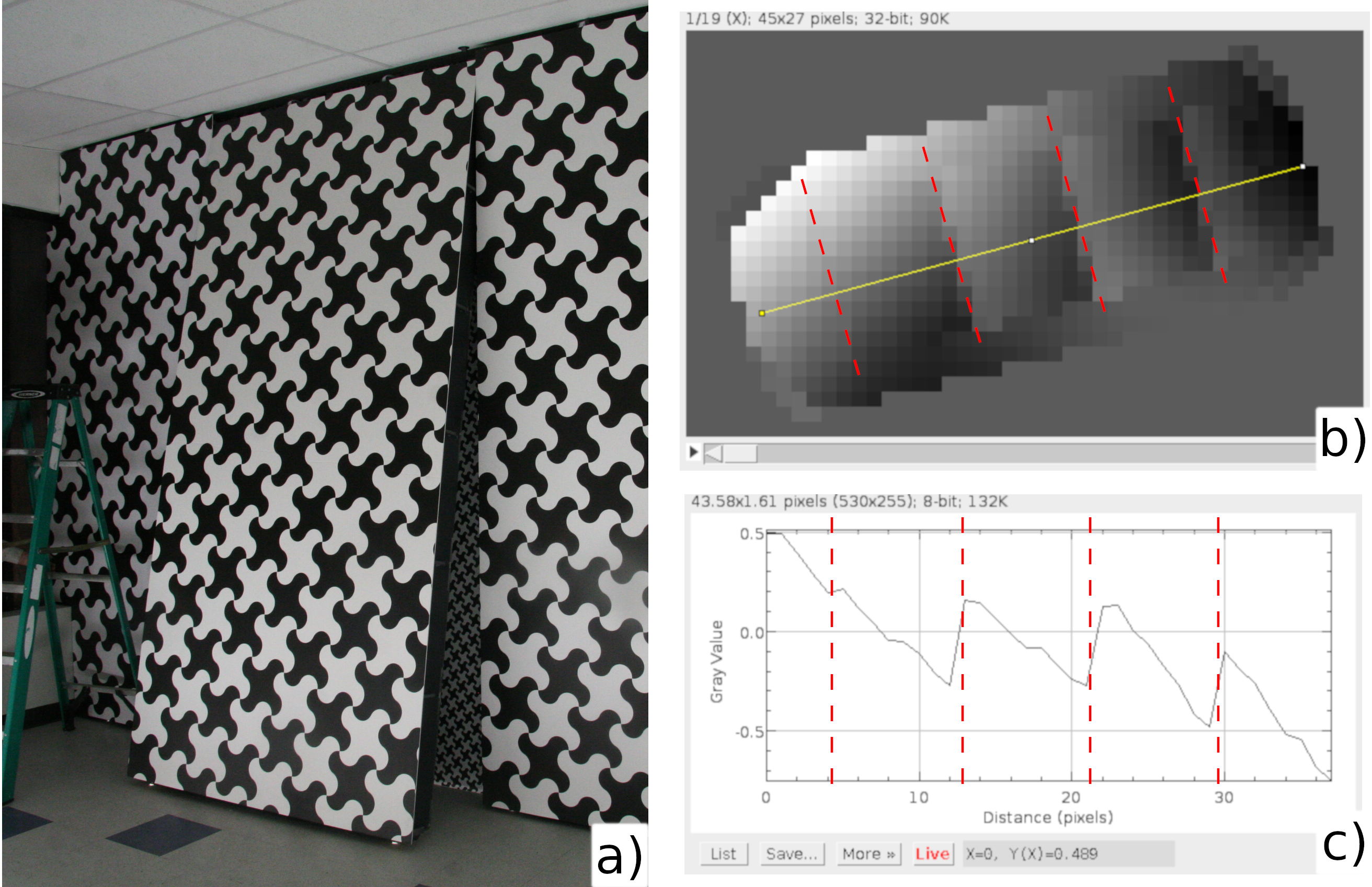
Figure 4: Refining pattern nodes coordinates: a) Mounting of the calibration pattern panels; b) Measured deviation of the nodes in the X direction (pixel values), tiles correspond to integer grid nodes indexes; c) Profile along the half-height of the pattern (vertical units are millimeters).

When the composite camera extrinsic parameters are determined from the visible range quadocular subsystem, intrinsic and extrinsic (relative to the composite camera) parameters of the LWIR modules are calculated.

The third calibration stage is fully automatic again. Here the space-variant PSFs are calculated for each sensor, each color channel and each of the overlapping by 50% $256\text{\times}256\text{\,}$ area of the RGB and $32\text{\times}32\text{\,}$ area of the LWIR image. These PSFs are subsequently inverted and used as deconvolution kernels to compensate optical aberrations of the lenses. The PSF kernels are calculated by co-processing of the acquired images and the synthetic ones generated by applying intrinsic and extrinsic parameters, and calibration pattern geometric corrections calculated in stage 2 to the ideal pattern model. In addition to accounting for the optical aberrations such as spherical or chromatic (for RGB modality), these kernels absorb deviations of the actual lens distortion from the radial model described by each sub-camera intrinsic parameters. This is especially important for the differential rectification (DR) proposed by Filippov [9].

2.4 Differential Rectification of the Stereo Images

While long range stereo depends on high disparity resolution, it does not need to process image sets with large disparities. There are other efficient algorithms for 3D reconstruction for shorter ranges, such as semi-global matching by Hirschmuller [15] that has field-programmable gate array (FPGA) and ASIC implementations. It is possible to combine the proposed long range approach with other algorithms to handle near objects.

DR is partial rectification of the stereo images to the common for all stereo set distortion model rather than full rectification to a rectilinear projection. When DR is applicable it avoids image re-sampling that either introduces sampling noise or requires up-sampling that leads to an increase in memory footprint and computational resources.

Limitations of the DR compared to the full rectification are estimated below, defining maximal disparity that can be processed as well as requirements to the camera lenses.

Considering the worst correlation case where patch data is all zero except at the very end ($w/2$ for 1-D correlation), disparity error $d_{err}$ caused by the scale mismatch $K_{diff}$ between the same object projection in two cameras is

$$d_{err}=\frac{K_{diff}\cdot w}{2}$$ (1)

and so for the specified disparity error

$$K_{diff}=\frac{2\cdot d_{err}}{w}$$ (2)

for $w=8pix$ and target error of $0.05pix$ $K_{diff}=1.25\%$.

There are two main sources of the $K_{diff}$ considering that the axes of the camera modules in a rig are properly aligned during factory calibration.

One of them, $K_{lens}$ depends on the differences between the lenses, primarily on their focal length and can be estimated as relative standard deviation (RSD) of the lens focal length $f$. In our case for the RGB subsystem $\lx@glossaries@gls@link{main}{rsd}{\leavevmode{\color[rgb]{0.23,0.27,0.29}{\color[rgb]{0.23,0.27,0.29}RSD}}}_{f}=0.027\%\ll 1.25\%$, for the LWIR subsystem $\lx@glossaries@gls@link{main}{rsd}{\leavevmode{\color[rgb]{0.23,0.27,0.29}{\color[rgb]{0.23,0.27,0.29}RSD}}}_{f}=1.7\%>1.25\%$ and may limit disparity resolution in some cases. $\lx@glossaries@gls@link{main}{rsd}{\leavevmode{\color[rgb]{0.23,0.27,0.29}{\color[rgb]{0.23,0.27,0.29}RSD}}}_{f}$ can be significantly improved in production by measuring and binning lenses to select matching ones for each rig. In our experiments, we did not have extra LWIR modules and had to use available ones.

Disparity term $K_{disp}$ depends on disparity value and the lens distortion. For the simple case of the barrel/pincushion distortion specified in percents $D_{perc}$, sensor FoV radius $r$ and disparity $d$ in pixels

$$K_{disp}=\frac{D_{perc}}{100\%}\cdot\frac{d}{r}$$ (3)

and so maximal disparity for which DR remains valid

$$d_{max}=r\cdot\frac{100\%}{D_{perc}}\cdot K_{disp}$$ (4)

For the RGB cameras $D_{perc}=10\%$, $r=1296~{}pix$ and so $d_{max}(RGB)=162~{}pix$, for LWIR $D_{perc}=15\%$, $r=80~{}pix$ and so $d_{max}(\lx@glossaries@gls@link{main}{lwir}{\leavevmode{\color[rgb]{0.23,0.27,0.29}{\color[rgb]{0.23,0.27,0.29}LWIR}}})=6.7~{}pix$.

FoV of the visible range cameras in the experimental rig is 20% larger than that of the LWIR one, and with the $16\times$ lower sensor resolution one LWIR pixel corresponds to 12.8 pixels of the RGB cameras, so maximal disparity of $6.7\text{\,}\mathrm{pix}$ corresponds for the same objects to $86.8~{}pix<d_{max}(RGB)=162~{}pix$ of the RGB cameras.

The above estimation proves that DR is justified for our experimental system with LWIR disparities up to $6.7\text{\,}\mathrm{pix}$ corresponding to the minimum object distance of $4.0\text{\,}\mathrm{m}$. Other existing algorithms may be employed to measure shorter distances, but it is possible to relax the above limitations of the DR for short distances. At a short distance, larger disparity errors are often acceptable as they cause smaller depth errors, and the images themselves will be degraded anyway by the depth of field limitation.

3. Experimental Setup, Image Sets Acquisition and Processing

3.1 Dual Quadocular Camera Rig

The experimental camera setup (Figure 1) consists of the rigidly assembled quadocular $2592\text{\times}1936\text{\,}$ RGB camera and another quadocular $160\text{\times}120\text{\,}$ LWIR one. The rig is mounted on a backpack frame, it is powered by a 48VDC Li Po battery providing several hours of operation.

The whole rig was calibrated as described in Sections 2.2, 2.3, using the DR method. Common sets of the intrinsic parameters were calculated separately for each of the two modalities. Residual deviations of the same modality cameras from the respective distortion models where absorbed by the 2D arrays of space-variant deconvolution kernels saved as the FD coefficients. Each of the 8 cameras was synchronized. Inter-modality offset was measured by the filming of the rotating object; the result was added to the color channels to compensate for the latency of the LWIR modules. FLIR Lepton 3.5 does not have provisions for external synchronization so we used the genlock approach with simultaneous reset and simultaneous radiometric calibration. The measured mismatch between the 4 modules was less than $10\text{\,}\mathrm{\SIUnitSymbolMicro s}$ and it did not change over tens of hours cameras were running without a reboot. Color cameras were configured to run in slave mode triggered by the LWIR ones, the whole system was operating at $9\text{\,}\mathrm{Hz}$ limited by Lepton modules.

3.2 Image Sets Acquisition

Image sets were recorded in raw mode to cameras internal SSD memory, 14 available bits of the LWIR data were recorded as Tiff files together with the provided telemetry metadata. Each image file name contains master camera timestamp and a channel number – this information allows to arranging of the image sets of 4 of RGB and 4 LWIR each for later processing. Image sets were captured in the natural environment and contain trees, rocks, snow patches, people and cars - parked and passing by at highway speed. Examples of both modality images are shown in Figure 5, more are available online [10] in an interactive table.

While processing the captured sets we found that the 3D-printed camera cases of the LWIR modules yielded under pressure of the tightened screws, and we perform field calibration of the extrinsic parameters. We captured far mounting ridges for the RGB modality calibration and used an RGB-derived depth map to calibrate the LWIR subsystem.

3.3 Image Sets Processing

Processing of each modality image quads is performed separately, it is based on the correlation of the $16\text{\times}16\text{\,}$ overlapping by 50% tiles. Subpixel disparity resolution for matching image patches maybe be influenced by the pixel-locking effect especially when the number of participating pixels is small. This effect is described for Particle Image Velocimetry (PIV) applications by Fincham and Spedding [12], Chen and Katz [5] proposed a method of reducing this effect for clusters over $4\text{\times}4\text{\,}$. Pixel locking for the stereo disparity may occur even for large patches: Shimizu and Okutomi [26] measured this effect by moving the target away from the camera and proposed a correction.

We use phase correlation for accurate subpixel matching of the image patches. DR eliminates sampling errors, the subpixel-accurate initial alignment of the patches is implemented by integer pixel shift followed by the transformation to the FD and phase rotation that is equivalent to the pixel domain shift. Phase correlation in the FD is proven to be free of pixel locking effect, Balci and Foroosh[1] implemented plane fitting to the FD view of the phase correlation. Hoge[16] calculated disparity from the phase correlation using the singular value decomposition (SVD) approach.

The overall method of depth map generation for both modalities involves a fast converging iterative process where the expected disparity is estimated for each depth sample, and this value is used for lossless calculation of the FD representation of the corresponding source images patches. This disparity estimation and corresponding pre-shift of the patches is analogous to the eye convergence in the human binocular vision. Initial disparity estimation methods depend on specific application – expected disparity may be calculated from the previous sample when a continuous video stream is available. Other methods use intra-scene neighbors or just simple but time-consuming disparity sweep. After the residual disparity is calculated from the correlation, the refined disparity is used in the next iteration step. There are 6 pairs to be correlated in the quadocular system. For the cameras located in the corners of a square, there are two horizontal pairs, two vertical ones and two diagonal. For the ground truth depth measurement with color cameras that have over $13\times$ higher resolution than the LWIR modality we combine those six 2D phase correlation results and calculate subpixel disparity by the polynomial approximation around the integer argmax. Figure 5b) shows one of the four color images and 5c) illustrates the disparity map calculated from it, subsequently used to derive the ground truth for LWIR subsystem evaluation and training/testing of the DNN.

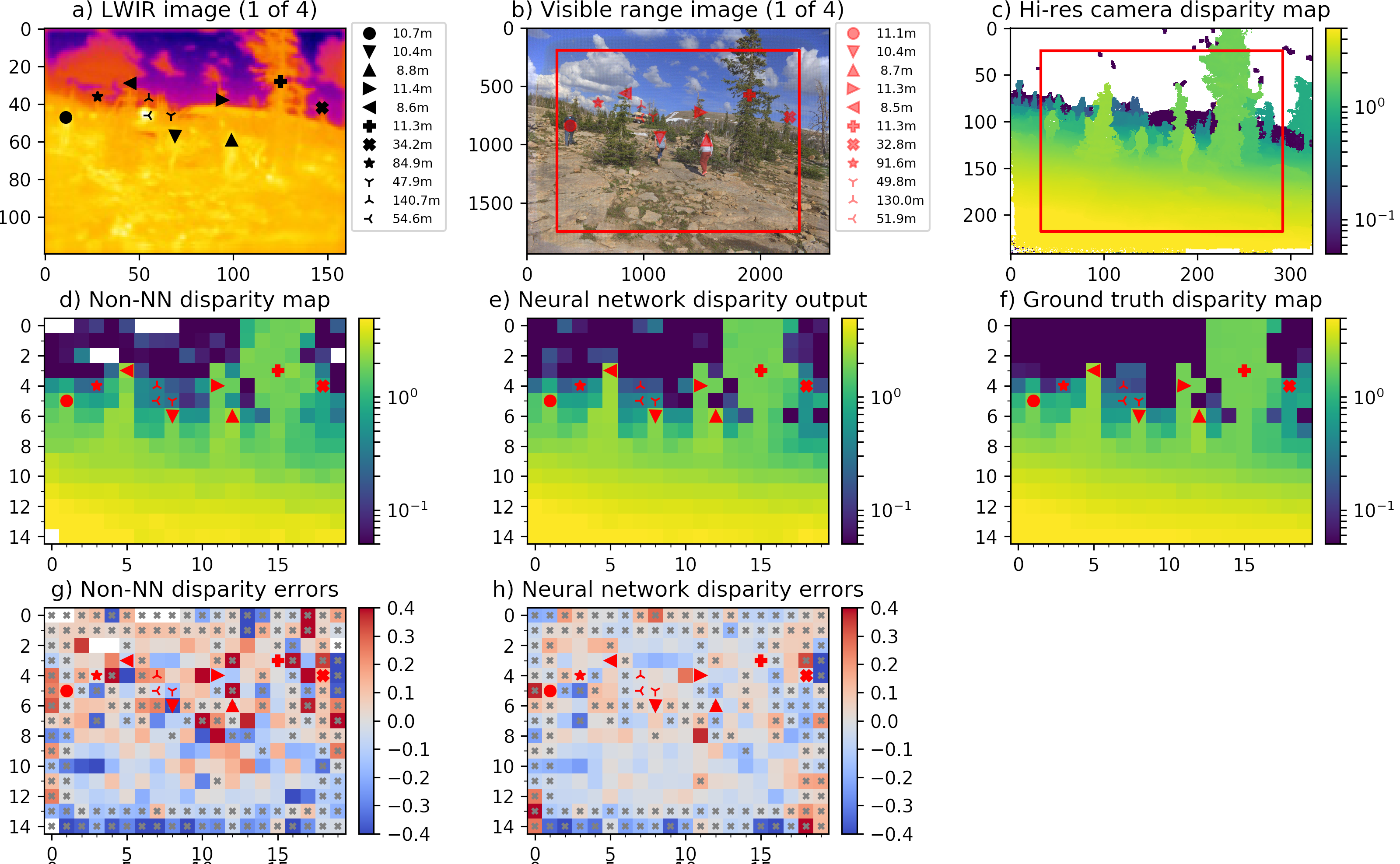
Figure 5: LWIR depth map generation and comparison to the ground truth data for Scene 7 listed in Table 1.

We used the same method as described above to process the 2D correlation outputs into the disparity map for the LWIR modality that is the subject of this research. Figure 5a) shows registered LWIR image in pseudo-colors, and 5d) – corresponding disparity map. Ground truth for LWIR shown in 5f) is calculated from the high-res disparity map 5c). As the resolution of the color modality depth map is higher than that of LWIR, multiple source tiles map to the same destination one. Many destination tiles fall on the edges and get data from both the FG and the BG objects. Averaging disparity values in the destination tiles would result in false objects at some intermediate between FG and BG disparity. Instead, the disparity data for each destination tile is sorted and if the distribution is found to be bimodal, only the larger disparity values corresponding to the FG object are preserved as the FG objects are more important in most cases.

3.4 Neural Network Training and Inference

The use of the DNNs for the fusion of the multimodal stereo images is now a popular approach, especially when the application area is defined in advance, e.g. DNN is used for pedestrian detection (Zhang et al. [35]). In our work, we do not target any specific scene types but rather aim to improve subpixel argmax of the 2D correlation, using a minimal amount of prior information - just that we need long range 3D perception. We adapted TPNET described by Filippov and Dzhimiev [11] to use with the LWIR camera. That adaptation gave us $2\times$ depth accuracy improvement over the NN-less method. Application-specific networks can be built on top of the proposed system. The network has two stages connected in series: the first stage consisting of 4 fully connected (FC) layers (256-128-32-16) with leaky ReLU activation for all but the last layer is fed with the correlation data from all pairs of a single tile together with the amount of applied pre-shift of the image patches; the second (convolutional with $5\times 5$ kernel, stride 1) stage receives $20\times 12\times 16$ output from the first stage and outputs $20\times 12$ disparity predictions. Such 2-stage architecture, where the first stage processes individual tiles separately, and the second one adds neighbors context improves training and reduces computations when only a small fraction of the input tiles are updated during iteration. The neighbors’ context is used to fill the gaps in the textureless areas and to follow the edges of the FG objects.

For training and corresponding testing, the network was reconfigured to a 25-head Siamese one with 25 instances of Stage 1 fed with $5\text{\times}5\text{\,}$ patches of correlation tiles data followed by a Stage 2 instance that outputs a single disparity prediction corresponding to the center tile of $5\text{\times}5\text{\,}$ input group. We used 1100 image sets split as 80%/20% for training and testing as a source of $5\text{\times}5\text{\,}$ tile clusters. For the cost function, we used the L2 norm weighted by the ground truth confidence and supplemented it by extra terms to improve prediction quality and training convergence. Typical 3D scene reconstructed from the long range stereo images when disparity resolution is insufficient to resolve depth variations across individual far objects can be better approximated by a set of fronto-parallel patches corresponding to different objects than by a smooth surface. The only common exception is the ground surface that is close to the line of sight, usually horizontal. When just the L2 cost is used the disparity prediction looks blurred. If the correlated tiles simultaneously contain both FG and BG features the result may correspond to the nonexistent object at intermediate range, it would be more useful if the prediction for such ambiguous tiles would be either FG or BG, so we added a cost term for the predictions falling between the FG and the BG.

Another cost terms were added to reduce overfitting. Stage 2 prediction for each tile depends on that tile data and the tiles around it (up to $\pm 2$) in each direction, and while these other tiles improve prediction by following edges and filling the low-textured gaps, in most cases just a single tile correlation data should provide reasonably good prediction, and being a much simpler network it is less prone to overfitting and plays regularization role when mixed to the cost function. We added two modified Stage 2 networks with the weights shared with the original Stage 2 – one with all but the center Stage 1 output zeroed out, the second one preserved inner $3\text{\times}3\text{\,}$ tile cluster. The L2 norms from these additional outputs are multiplied by hyperparameters and added to the cost function, output disparity prediction still uses only the full $5\text{\times}5\text{\,}$ Stage 2 outputs.

After the network was trained and tested on the $5\text{\times}5\text{\,}$ tile clusters without a larger context we manually selected a 19-scene subset of the test image sets. These scenes represent different objects (people, trees, rocks, parked and moving cars), with or without significant motion blur during image capturing. In addition to the calculation of the root mean square error (RMSE) for all sets, we marked some features of interest and evaluated the measured distance. RMSE calculated for the whole image would be dominated by the ambiguity in the attribution of the FG tiles to the BG (or vice versa) for the tiles on the object edges, so we removed 10% outliers from each scene in Table 1. This table lists LWIR disparity errors calculated directly from the interpolated argmax of combined 2D phase correlation tiles in column 3, the last column contains errors of the network prediction.

#	Scene timestamp	Non-DNN disparity RMSE (pix)	DNN disparity RMSE (pix)
1	1562390202.933097	0.136	0.060
2	1562390225.269784	0.147	0.065
3	1562390225.839538	0.196	0.105
4	1562390243.047919	0.136	0.060
5	1562390251.025390	0.152	0.074
6	1562390257.977146	0.146	0.074
7	1562390260.370347	0.122	0.058
8	1562390260.940102	0.135	0.064
9	1562390317.693673	0.157	0.078
10	1562390318.833313	0.136	0.065
11	1562390326.354823	0.144	0.090
12	1562390331.483132	0.209	0.100
13	1562390333.192523	0.153	0.067
14	1562390402.254007	0.140	0.077
15	1562390407.382326	0.130	0.065
16	1562390409.661607	0.113	0.063
17	1562390435.873048	0.153	0.057
18	1562390456.842237	0.211	0.102
19	1562390460.261151	0.201	0.140
	Average	0.154	0.077

Table 1: Disparity RMSE calculated between LWIR and pseudo-ground truth data measured with high resolution visible range cameras for 90% of the depth samples. Traditional (non-DNN) and DNN results are presented. Scene 7 details are shown in Figure 5.

Figure 5 illustrates Scene 7 (shown in bold in Table 1), other listed scenes with animated views are available online [10]. Scenes 3 and 5 were captured with large horizontal motion blur, scenes 18 and 19 contain objects closer than the near clipping plane for disparities.

4. Discussion

Similar to other researches who work in the area of LWIR 3D perception we had to develop a multimodal camera rig to register ground truth data, develop the calibration pattern, capture and process imagery. There are multimodal stereo image sets available, such as Treible et al. [30] that they subsequently used for WILDCAT network development Treible et al. [29] and LITIV (Bilodeau et al. [3]) with annotated human silhouettes. These benchmark datasets are very useful for evaluation of higher-level DNNs, but they assume specific calibration methods and so are not suitable for comparison of end-to-end systems that mix hardware, calibration, and software components. The ultimate test of the 3D perception system is how well it performs its task, how reliable is the autonomous driving, but such tests (Zapf et al. [34]) require specific test sites and so are difficult to reproduce when different hardware is involved.

Comparison of just the calibration methods has its limitations too – measured MRE value may be misleading when not verified by the actual disparity accuracy in 3D scene reconstruction performed independently from the calibration. This is why the calibration quality is often evaluated by the accuracy of the stereo 3D reconstruction, with the result presented as disparity resolution in pixels – parameter that is invariant of the sensor resolution, focal length to pixel size ratio (angular resolution), and the camera baseline.

We follow this path and compare our results with those published in Lee et al. [18]. They used a pair of the FLIR Tau 11 $640\text{\times}512\text{\,}$ cameras at a baseline of $0.75\text{\,}\mathrm{m}$ with the ground truth data provided by a LIDAR. During processing, they used a two-level representation with L0 having full $640\text{\times}512\text{\,}$ resolution and L1 – reduced to $320\text{\times}256\text{\,}$. They compared theoretical models of range accuracy for distances of up to $40\text{\,}\mathrm{m}$ range for $0.25\text{\,}\mathrm{pix}$ disparity resolution of L0 and L1 and the measured range accuracy at up to $25\text{\,}\mathrm{m}$, their graphs show match for L1 with $0.25\text{\,}\mathrm{pix}$ resolution, corresponding to $0.5\text{\,}\mathrm{pix}$ of the registered images. Our results are $0.154\text{\,}\mathrm{pix}$ with polynomial argmax interpolation and $0.077\text{\,}\mathrm{pix}$ with a trained DNN– 6.5 times improvement. While our system uses lower resolution LWIR sensors, the dual-modal calibration method, and quadocular camera design demonstrate that disparity accuracy in pixels remains approximately constant even for much higher resolution visible range cameras.

Comparison of our disparity density results with their published disparity map examples (63%-70.5%) shows our system advantage (Table 1 summarizes 90% of the best tiles), but such comparison is less strict as the density is highly dependent on the scene details.

5. Acknowledgments

We thank Tolga Tasdizen for his suggestions on the network architecture and implementation. This work is funded by SBIR Contract FA8652-19-P-WI19 (topic AF191-010).

References

- [1] Murat Balci and Hassan Foroosh. Inferring motion from the rank constraint of the phase matrix. In Acoustics, Speech, and Signal Processing, 2005. Proceedings.(ICASSP’05). IEEE International Conference on, volume 2, pages ii–925. IEEE, 2005.
- [2] Axel Beauvisage and Nabil Aouf. Low cost and low power multispectral thermal-visible calibration. In 2017 IEEE SENSORS, pages 1–3. IEEE, 2017.
- [3] Guillaume-Alexandre Bilodeau, Atousa Torabi, Pierre-Luc St-Charles, and Dorra Riahi. Thermal–visible registration of human silhouettes: A similarity measure performance evaluation. Infrared Physics & Technology, 64:79–86, 2014.
- [4] Yanpeng Cao, Baobei Xu, Zhangyu Ye, Jiangxin Yang, Yanlong Cao, Christel-Loic Tisse, and Xin Li. Depth and thermal sensor fusion to enhance 3D thermographic reconstruction. Optics express, 26(7):8179–8193, 2018.
- [5] J Chen and J Katz. Elimination of peak-locking error in piv analysis using the correlation mapping method. Measurement Science and Technology, 16(8):1605, 2005.
- [6] G Chernov, V Chernov, and M Barboza Flores. 3D dynamic thermography system for biomedical applications. In Application of Infrared to Biomedical Sciences, pages 517–545. Springer, 2017.
- [7] Andreas Ellmauthaler, Eduardo AB da Silva, Carla L Pagliari, Jonathan N Gois, and Sergio R Neves. A novel iterative calibration approach for thermal infrared cameras. In 2013 IEEE International Conference on Image Processing, pages 2182–2186. IEEE, 2013.
- [8] Andreas Ellmauthaler, Carla L Pagliari, Eduardo AB da Silva, Jonathan N Gois, and Sergio R Neves. A visible-light and infrared video database for performance evaluation of video/image fusion methods. Multidimensional Systems and Signal Processing, 30(1):119–143, 2019.
- [9] Andrey Filippov. Method for the FPGA-based long range multi-view stereo with differential image rectification, Sept. 14 2018. US Patent App. 16/132,343.
- [10] Andrey Filippov. TPNET with LWIR. https://blog.elphel.com/2019/08/tpnet-with-lwir/, 2019. Technical blog post.
- [11] Andrey Filippov and Oleg Dzhimiev. See far with TPNET: a tile processor and a CNN symbiosis. arXiv preprint arXiv:1811.08032, 2018.
- [12] AM Fincham and GR Spedding. Low cost, high resolution dpiv for measurement of turbulent fluid flow. Experiments in Fluids, 23(6):449–462, 1997.
- [13] Michael Gschwandtner, Roland Kwitt, Andreas Uhl, and Wolfgang Pree. Infrared camera calibration for dense depth map construction. In 2011 IEEE Intelligent Vehicles Symposium (IV), pages 857–862. IEEE, 2011.
- [14] Josh Harguess and Shawn Strange. Infrared stereo calibration for unmanned ground vehicle navigation. In Unmanned Systems Technology XVI, volume 9084, page 90840S. International Society for Optics and Photonics, 2014.
- [15] Heiko Hirschmuller. Accurate and efficient stereo processing by semi-global matching and mutual information. In Computer Vision and Pattern Recognition, 2005. CVPR 2005. IEEE Computer Society Conference on, volume 2, pages 807–814. IEEE, 2005.
- [16] William Scott Hoge. A subspace identification extension to the phase correlation method [mri application]. IEEE transactions on medical imaging, 22(2):277–280, 2003.
- [17] Miklas Kristoffersen, Jacob Dueholm, Rikke Gade, and Thomas Moeslund. Pedestrian counting with occlusion handling using stereo thermal cameras. Sensors, 16(1):62, 2016.
- [18] Daren Lee, Arturo Rankin, Andres Huertas, Jeremy Nash, Gaurav Ahuja, and Larry Matthies. LWIR passive perception system for stealthy unmanned ground vehicle night operations. In Unmanned Systems Technology XVIII, volume 9837, page 98370D. International Society for Optics and Photonics, 2016.
- [19] Yan Li, Jindong Tan, Yinlong Zhang, Wei Liang, and Hongsheng He. Spatial calibration for thermal-rgb cameras and inertial sensor system. In 2018 24th International Conference on Pattern Recognition (ICPR), pages 2295–2300. IEEE, 2018.
- [20] Ben Miethig, Ash Liu, Saeid Habibi, and Martin v Mohrenschildt. Leveraging thermal imaging for autonomous driving. In 2019 IEEE Transportation Electrification Conference and Expo (ITEC), pages 1–5. IEEE, 2019.
- [21] Harry Ng, R Du, et al. Acquisition of 3D surface temperature distribution of a car body. In 2005 IEEE International Conference on Information Acquisition, pages 5–pp. IEEE, 2005.
- [22] Surya Prakash, Pei Yean Lee, and Terry Caelli. 3D mapping of surface temperature using thermal stereo. In 2006 9th International Conference on Control, Automation, Robotics and Vision, pages 1–4. IEEE, 2006.
- [23] Johannes Rangel, Samuel Soldan, and A Kroll. 3D thermal imaging: Fusion of thermography and depth cameras. In International Conference on Quantitative InfraRed Thermography, 2014.
- [24] Arturo Rankin, Andres Huertas, Larry Matthies, Max Bajracharya, Christopher Assad, Shane Brennan, Paolo Bellutta, and Gary W Sherwin. Unmanned ground vehicle perception using thermal infrared cameras. In Unmanned Systems Technology XIII, volume 8045, page 804503. International Society for Optics and Photonics, 2011.
- [25] Philip Saponaro, Scott Sorensen, Stephen Rhein, and Chandra Kambhamettu. Improving calibration of thermal stereo cameras using heated calibration board. In 2015 IEEE International Conference on Image Processing (ICIP), pages 4718–4722. IEEE, 2015.
- [26] Masao Shimizu and Masatoshi Okutomi. Sub-pixel estimation error cancellation on area-based matching. International Journal of Computer Vision, 63(3):207–224, 2005.
- [27] Karolj Skala, Tomislav Lipić, Ivan Sović, Luko Gjenero, and Ivan Grubišić. 4d thermal imaging system for medical applications. Periodicum biologorum, 113(4):407–416, 2011.
- [28] L St-Laurent, M Mikhnevich, A Bubel, and D Prévost. Passive calibration board for alignment of VIS-NIR, SWIR and LWIR images. Quantitative InfraRed Thermography Journal, 14(2):193–205, 2017.
- [29] Wayne Treible, Philip Saponaro, and Chandra Kambhamettu. Wildcat: In-the-wild color-and-thermal patch comparison with deep residual pseudo-siamese networks. In 2019 IEEE International Conference on Image Processing (ICIP), pages 1307–1311. IEEE, 2019.
- [30] Wayne Treible, Philip Saponaro, Scott Sorensen, Abhishek Kolagunda, Michael O’Neal, Brian Phelan, Kelly Sherbondy, and Chandra Kambhamettu. Cats: A color and thermal stereo benchmark. In Proceedings of the IEEE Conference on Computer Vision and Pattern Recognition, pages 2961–2969, 2017.
- [31] Stephen Vidas, Ruan Lakemond, Simon Denman, Clinton Fookes, Sridha Sridharan, and Tim Wark. A mask-based approach for the geometric calibration of thermal-infrared cameras. IEEE Transactions on Instrumentation and Measurement, 61(6):1625–1635, 2012.
- [32] Stephen Vidas and Peyman Moghadam. Heatwave: A handheld 3D thermography system for energy auditing. Energy and Buildings, 66:445–460, 2013.
- [33] Rongqian Yang, Wei Yang, Yazhu Chen, and Xiaoming Wu. Geometric calibration of ir camera using trinocular vision. Journal of Lightwave technology, 29(24):3797–3803, 2011.
- [34] Josh Zapf, Gaurav Ahuja, Jeremie Papon, Daren Lee, Jeremy Nash, and Arturo Rankin. A perception pipeline for expeditionary autonomous ground vehicles. In Unmanned Systems Technology XIX, volume 10195, page 101950F. International Society for Optics and Photonics, 2017.
- [35] Lu Zhang, Xiangyu Zhu, Xiangyu Chen, Xu Yang, Zhen Lei, and Zhiyong Liu. Weakly aligned cross-modal learning for multispectral pedestrian detection. In Proceedings of the IEEE International Conference on Computer Vision, pages 5127–5137, 2019.
- [36] Zhengyou Zhang. A flexible new technique for camera calibration. IEEE Transactions on pattern analysis and machine intelligence, 22, 2000.
- [37] Yannick Wend Kuni Zoetgnandé, Alain-Jérôme Fougères, Geoffroy Cormier, and Jean-Louis Dillenseger. Robust low resolution thermal stereo camera calibration. In Eleventh International Conference on Machine Vision (ICMV 2018), volume 11041, page 110411D. International Society for Optics and Photonics, 2019.