Inductive Relation Prediction by Subgraph Reasoning

Abstract

The dominant paradigm for relation prediction in knowledge graphs involves learning and operating on latent representations (i.e., embeddings) of entities and relations. However, these embedding-based methods do not explicitly capture the compositional logical rules underlying the knowledge graph, and they are limited to the transductive setting, where the full set of entities must be known during training. Here, we propose a graph neural network based relation prediction framework, GraIL, that reasons over local subgraph structures and has a strong inductive bias to learn entity-independent relational semantics. Unlike embedding-based models, GraIL is naturally inductive and can generalize to unseen entities and graphs after training. We provide theoretical proof and strong empirical evidence that GraIL can represent a useful subset of first-order logic and show that GraIL outperforms existing rule-induction baselines in the inductive setting. We also demonstrate significant gains obtained by ensembling GraIL with various knowledge graph embedding methods in the transductive setting, highlighting the complementary inductive bias of our method.

1 Introduction

Knowledge graphs (KGs) are a collection of facts which specify relations (as edges) among a set of entities (as nodes). Predicting missing facts in KGs—usually framed as relation prediction between two entities—is a widely studied problem in statistical relational learning (Nickel et al., 2016).

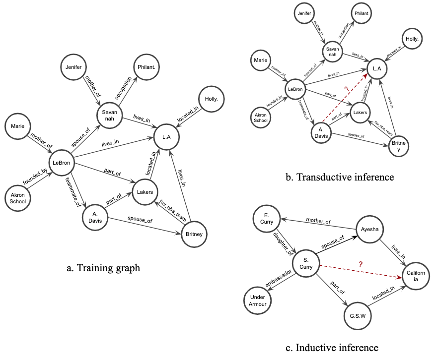
Figure 1: Illustration of transductive and inductive settings for relation prediction in knowledge graphs.

The most dominant paradigm, in recent times, has been to learn and operate on latent representations (i.e., embeddings) of entities and relations. These methods condense each entity’s neighborhood connectivity pattern into an entity-specific low-dimensional embedding, which can then be used to predict missing edges (Bordes et al., 2013; Trouillon et al., 2017; Dettmers et al., 2018; Sun et al., 2019). For example, in Figure 1a, the embeddings of LeBron and A.Davis will contain the information that they are both part of the Lakers organization, which could later be retrieved to predict that they are teammates. Similarly, the pattern that anyone closely associated with the Lakers would live in L.A with high probability could be encoded in the embedding space. Embedding-based methods have enjoyed great success by exploiting such local connectivity patterns and homophily. However, it is not clear if they effectively capture the relational semantics of knowledge graphs—i.e., the logical rules that hold among the relations underlying the knowledge graph.

Indeed, the relation prediction task can also be viewed as a logical induction problem, where one seeks to derive probabilistic logical rules (horn clauses) underlying a given KG. For example, from the KG shown in Figure 1a one can derive the simple rule

$$\exists Y.(X,\texttt{spouse\_of},Y)\wedge(Y,\texttt{lives\_in},Z)\\ \rightarrow(X,\texttt{lives\_in},Z).$$ (1)

Using the example from Figure 1b, this rule can predict the relation (A.Davis, lives_in, L.A). While the embedding-based methods encode entity-specific neighborhood information into an embedding, these logical rules capture entity-independent relational semantics.

One of the key advantages of learning entity-independent relational semantics is the inductive ability to generalise to unseen entities. For example, the rule in Equation (1) can naturally generalize to the unseen KG in Fig 1c and predict the relation (S.Curry, lives_in, California).

Whereas embedding-based approaches inherently assume a fixed set of entities in the graph—an assumption that is generally referred to as the transductive setting (Figure 1) (Yang et al., 2016)—in many cases, we seek algorithms with the inductive capabilities afforded by inducing entity-independent logical rules. Many real-world KGs are ever-evolving, with new nodes or entities being added over time—e.g., new users and products on e-commerce platforms or new molecules in biomedical knowledge graphs— the ability to make predictions on such new entities without expensive re-training is essential for production-ready machine learning models. Despite this crucial advantage of rule induction methods, they suffer from scalability issues and lack the expressive power of embedding-based approaches.

Present work. We present a Graph Neural Network (GNN) (Scarselli et al., 2008; Bronstein et al., 2017) framework (GraIL: Graph Inductive Learning) that has a strong inductive bias to learn entity-independent relational semantics. In our approach, instead of learning entity-specific embeddings we learn to predict relations from the subgraph structure around a candidate relation. We provide theoretical proof and strong empirical evidence that GraIL can represent logical rules of the kind presented above (e.g., Equation (1)). Our approach naturally generalizes to unseen nodes, as the model learns to reason over subgraph structures independent of any particular node identities.

In addition to the GraIL framework, we also introduce a series of benchmark tasks for the inductive relation prediction problem. Existing benchmark datasets for knowledge graph completion are set up for transductive reasoning, i.e., they ensure that all entities in the test set are present in the training data. Thus, in order to test models with inductive capabilities, we construct several new inductive benchmark datasets by carefully sampling subgraphs from diverse knowledge graph datasets. Extensive empirical comparisons on these novel benchmarks demonstrate that GraIL is able to substantially outperform state-of-the-art inductive baselines, with an average relative performance increase of $5.25\%$ and $6.75\%$ in AUC-PR and Hits@10, respectively, compared to the strongest inductive baseline.

Finally, we compare GraIL against existing embedding-based models in the transductive setting. In particular, we hypothesize that our approach has an inductive bias that is complementary to the embedding-based approaches, and we investigate the power of ensembling GraIL with embedding-based methods. We find that ensembling with GraIL leads to significant performance improvements in this setting.

2 Related Work

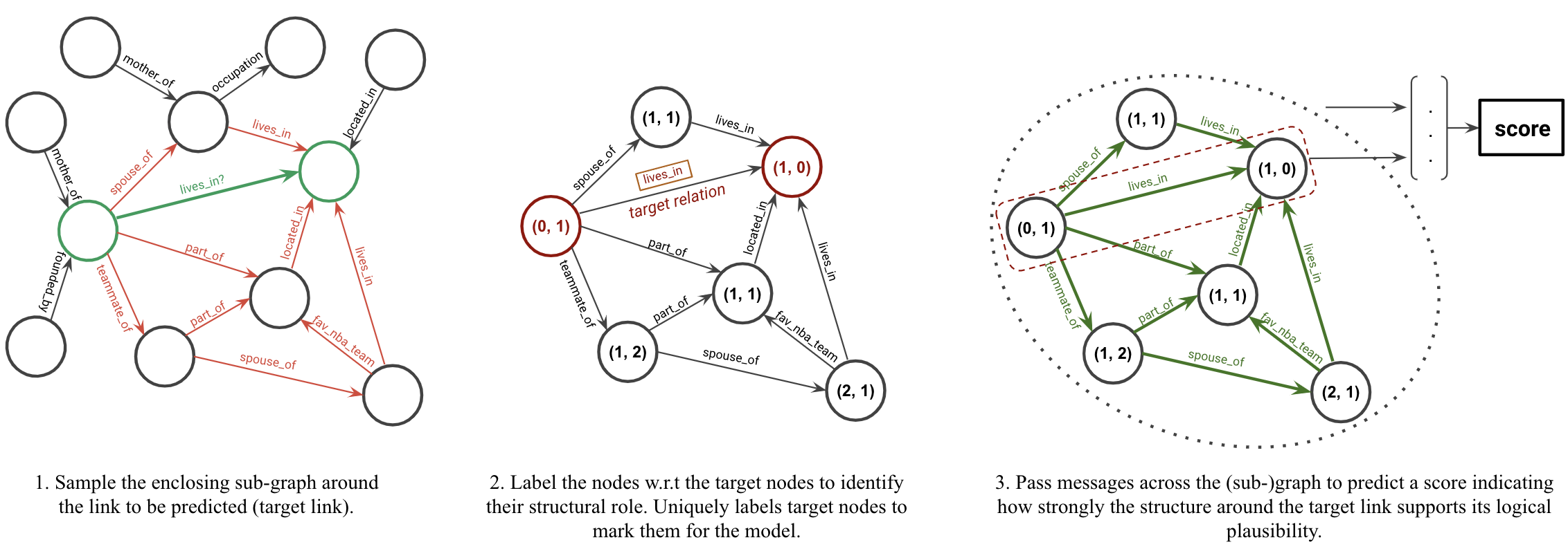
Figure 2: Visual illustration of GraIL for inductive relation prediction.

Embedding-based models. As noted earlier, most existing KG completion methods fall under the embedding-based paradigm. RotatE (Sun et al., 2019), ComplEx (Trouillon et al., 2017), ConvE (Dettmers et al., 2018) and TransE (Bordes et al., 2013) are some of the representative methods that train shallow embeddings (Hamilton et al., 2017a) for each node in the training set, such that these low-dimensional embeddings can retrieve the relational information of the graph. Our approach embodies an alternative inductive bias to explicitly encode structural rules. Moreover, while our framework is naturally inductive, adapting the embedding methods to make predictions in the inductive setting requires expensive re-training of embeddings for the new nodes.

Similar to our approach, the R-GCN model uses a GNN to perform relation prediction (Schlichtkrull et al., 2017). Although this approach, as originally proposed, is transductive in nature, it has the potential for inductive capabilities if given some node features (Hamilton et al., 2017b). Unlike our approach though, R-GCN still requires learning node-specific embeddings, whereas we treat relation prediction as a subgraph reasoning problem.

Inductive embeddings. There have been promising works for generating embeddings for unseen nodes, though they are limited in some ways. Hamilton et al. (2017b) and Bojchevski & Günnemann (2018) rely on the presence of node features which are not present in many KGs. (Wang et al., 2019) and (Hamaguchi et al., 2017) learn to generate embeddings for unseen nodes by aggregating neighboring node embeddings using GNNs. However, both of these approaches need the new nodes to be surrounded by known nodes and can not handle entirely new graphs.

Rule-induction methods. Unlike embedding-based methods, statistical rule-mining approaches induce probabilistic logical-rules by enumerating statistical regularities and patterns present in the knowledge graph (Meilicke et al., 2018; Galárraga et al., 2013). These methods are inherently inductive since the rules are independent of node identities, but these approaches suffer from scalability issues and lack expressive power due to their rule-based nature. Motivated by these statistical rule-induction approaches, the NeuralLP model learns logical rules from KGs in an end-to-end differentiable manner (Yang et al., 2017) using TensorLog (Cohen, 2016) operators. Building on NeuralLP, Sadeghian et al. (2019) recently proposed DRUM, which learns more accurate rules. This set of methods constitute our baselines in the inductive setting.

Link prediction using GNNs. Finally, outside of the KG literature, Zhang & Chen (2018) have theoretically proven that GNNs can learn common graph heuristics for link prediction in simple graphs. Zhang & Chen (2020) have used a similar approach to achieve competitive results on inductive matrix completion. Our proposed approach can be interpreted as an extension of Zhang & Chen (2018)s’ method to directed multi-relational knowledge graphs.

3 Proposed Approach

The key idea behind our approach is to predict relation between two nodes from the subgraph structure around those two nodes. Our method is built around the Graph Neural Network (GNN) (Hamilton et al., 2017a) (or Neural Message Passing (Gilmer et al., 2017)) formalism. We do not use any node attributes in order to test GraIL’s ability to learn and generalize solely from structure. Since it only ever receives structural information (i.e., the subgraph structure and structural node features) as input, the only way GraIL can complete the relation prediction task is to learn the structural semantics that underlie the knowledge graph. The overall task is to score a triplet $(u,r_{t},v)$, i.e., to predict the likelihood of a possible relation $r_{t}$ between a head node $u$ and tail node $v$ in a KG, where we refer to nodes $u$ and $v$ as target nodes and to $r_{t}$ as the target relation. Our approach to scoring such triplets can be roughly divided into three sub-tasks (which we detail below): (i) extracting the enclosing subgraph around the target nodes, (ii) labeling the nodes in the extracted subgraph, and (iii) scoring the labeled subgraph using a GNN (Figure 2).

3.1 Model Details

Step 1: subgraph extraction. We assume that local graph neighborhood of a particular triplet in the KG will contain the logical evidence needed to deduce the relation between the target nodes. In particular, we assume that the paths connecting the two target nodes contain the information that could imply the target relation. Hence, as a first step, we extract the enclosing subgraph around the target nodes. We define the enclosing subgraph between nodes $u$ and $v$ as the graph induced by all the nodes that occur on a path between $u$ and $v$. It is given by the intersection of neighbors of the two target nodes followed by a pruning procedure. More precisely, let $\mathcal{N}_{k}(u)$ and $\mathcal{N}_{k}(v)$ be set of nodes in the $k$-hop (undirected) neighborhood of the two target nodes in the KG. We compute the enclosing subgraph by taking the intersection, $\mathcal{N}_{k}(u)\cap\mathcal{N}_{k}(v)$, of these $k$-hop neighborhood sets and then prune nodes that are isolated or at a distance greater than $k$ from either of the target nodes. Following the Observation 1, this would give us all the nodes that occur on a path of length at most $k+1$ between nodes $u$ and $v$.

Observation 1. In any given graph, let the nodes on a path of length $\lambda$ between two different nodes $x$ and $y$ constitute the set $P_{xy}(\lambda)$. The maximum distance of any node on such a path, $v\in P_{xy}(\lambda)$, from either $x$ or $y$ is $\lambda-1$.

Note that while extracting the enclosing subgraph we ignore the direction of the edges. However, the direction is preserved while passing messages with Graph Neural Network, a point re-visited later. Also, the target tuple/edge $(u,r_{t},v)$ is added to the extracted subgraph to enable message passing between the two target nodes.

Step 2: Node labeling. GNNs require a node feature matrix, $\mathbf{X}\in\mathbb{R}^{|\mathcal{V}|\times d_{i}}$, as input, which is used to initialize the neural message passing algorithm (Gilmer et al., 2017). Since we do not assume any node attributes in our input KGs, we follow Zhang & Chen (2018) and extend their double radius vertex labeling scheme to our setting. Each node, $i$, in the subgraph around nodes $u$ and $v$ is labeled with the tuple $(d(i,u),d(i,v))$, where $d(i,u)$ denotes the shortest distance between nodes $i$ and $u$ without counting any path through $v$ (likewise for $d(i,v)$). This captures the topological position of each node with respect to the target nodes and reflects its structural role in the subgraph. The two target nodes, $u$ and $v$, are uniquely labeled $(0,1)$ and $(1,0)$ so as to be identifiable by the model. The node features are thus $[\text{one-hot}(d(i,u))\oplus\text{one-hot}(d(i,v))]$, where $\oplus$ denotes concatenation of two vectors. Note that as a consequence of Observation 1, the dimension of node features constructed this way is bounded by the number of hops considered while extracting the enclosing subgraph.

Step 3: GNN scoring. The final step in our framework is to use a GNN to score the likelihood of tuple $(u,r_{t},v)$ given $\mathcal{G}_{(u,v,r_{t})}$—the extracted and labeled subgraph around the target nodes. We adopt the general message-passing scheme described in Xu et al. (2019) where a node representation is iteratively updated by combining it with aggregation of it’s neighbors’ representation. In particular, the $k^{th}$ layer of our GNN is given by,

$$\mathbf{a}_{t}^{k} =\text{AGGREGATE}^{k}\left(\left\{\mathbf{h}_{s}^{k-1}:s\in\mathcal{N}(t)\right\},\mathbf{h}^{k-1}_{t}\right),$$ (2)

$$\mathbf{h}_{t}^{k} =\text{COMBINE}^{k}\left(\mathbf{h}_{t}^{k-1},\mathbf{a}_{t}^{k}\right),$$ (3)

where $\mathbf{a}_{t}^{k}$ is the aggregated message from the neighbors, $\mathbf{h}_{t}^{k}$ denotes the latent representation of node $t$ in the $k$-th layer, and $\mathcal{N}(t)$ denotes the set of immediate neighbors of node $t$. The initial latent node representation of any node $i$, $\mathbf{h}_{i}^{0}$, is initialized to the node features, $\mathbf{X}_{i}$, built according to the labeling scheme described in Step 2. This framework gives the flexibility to plug in different AGGREGATE and COMBINE functions resulting in various GNN architectures.

Inspired by the multi-relational R-GCN (Schlichtkrull et al., 2017) and edge attention, we define our AGGREGATE function as

$$\mathbf{a}_{t}^{k}=\sum_{r=1}^{R}\sum_{s\in\mathcal{N}_{r}(t)}\alpha_{rr_{t}st}^{k}\mathbf{W}_{r}^{k}\mathbf{h}_{s}^{k-1},$$

where $R$ is the total number of relations present in the knowledge graph; $\mathcal{N}_{r}(t)$ denotes the immediate outgoing neighbors of node $t$ under relation $r$; $\mathbf{W}_{r}^{k}$ is the transformation matrix used to propagate messages in the $k$-th layer over relation $r$; $\alpha_{rr_{t}st}^{k}$ is the edge attention weight at the $k$-th layer corresponding to the edge connecting nodes $s$ and $t$ via relation $r$. This attention weight, a function of the source node $t$, neighbor node $s$, edge type $r$ and the target relation to be predicted $r_{t}$, is given by

$$\mathbf{s} =\text{ReLU}\left(\mathbf{A}_{1}^{k}[\mathbf{h}_{s}^{k-1}\oplus\mathbf{h}_{t}^{k-1}\oplus\mathbf{e}_{r}^{a}\oplus\mathbf{e}_{r_{t}}^{a}]+\mathbf{b}_{1}^{k}\right)$$

$$\alpha_{rr_{t}st}^{k} =\sigma\left(\mathbf{A}_{2}^{k}\mathbf{s}+\mathbf{b}_{2}^{k}\right).$$

Here $\mathbf{h}^{k}_{s}$ and $\mathbf{h}^{k}_{t}$ denote the latent node representation of respective nodes at $k$-th layer of the GNN, $\mathbf{e}_{r}^{a}$ and $\mathbf{e}_{r_{t}}^{a}$ denote learned attention embeddings of respective relations. Note that the attention weights are not normalized and instead come out of a sigmoid gate which regulates the information aggregated from each neighbor. As a regularization measure, we adopt the basis sharing mechanism, introduced by (Schlichtkrull et al., 2017), among the transformation matrices of each layer, $\mathbf{W}_{r}^{k}$. We also implement a form of edge dropout, where edges are randomly dropped from the graph while aggregating information from the neighborhood.

The COMBINE function that yielded the best results is also derived from the R-GCN architecture. It is given by

$$\mathbf{h}_{t}^{k}=\text{ReLU}\left(\mathbf{W}_{self}^{k}\mathbf{h}_{t}^{k-1}+\mathbf{a}_{t}^{k}\right).$$ (4)

With the GNN architecture as described above, we obtain the node representations after $L$ layers of message passing. A subgraph representation of $\mathcal{G}_{(u,v,r_{t})}$ is obtained by average-pooling of all the latent node representations:

$$\mathbf{h}^{L}_{\mathcal{G}_{(u,v,r_{t})}}=\frac{1}{|\mathcal{V}|}\sum_{i\in\mathcal{V}}\mathbf{h}_{i}^{L},$$ (5)

where $\mathcal{V}$ denotes the set of vertices in graph $\mathcal{G}_{(u,v,r_{t})}$.

Finally, to obtain the score for the likelihood of a triplet $(u,r_{t},v)$, we concatenate four vectors—the subgraph representation ($\mathbf{h}^{L}_{\mathcal{G}_{(u,v,r_{t})}}$), the target nodes’ latent representations ($\mathbf{h}^{L}_{u}$ and $\mathbf{h}^{L}_{v}$), and a learned embedding of the target relation ($\mathbf{e}_{r_{t}}$)—and pass these concatenated representations through a linear layer:

$$\text{score}(u,r_{t},v)=\mathbf{W}^{T}[\mathbf{h}^{L}_{\mathcal{G}_{(u,v,r_{t})}}\oplus\mathbf{h}^{L}_{u}\oplus\mathbf{h}^{L}_{v}\oplus\mathbf{e}_{r_{t}}].$$ (6)

In our best performing model, in addition to using the node representations from the last layer, we also make use of representations from intermittent layers. This is inspired by the JK-connection mechanism introduced by Xu et al. (2018), which allows for flexible neighborhood ranges for each node. Addition of such JK-connections made our model’s performance robust to the number of layers of the GNN. Precise implementation details of basis sharing, JK-connections and other model variants that were experimented with can be found in the Appendix.

3.2 Training Regime

Following the standard and successful practice, we train the model to score positive triplets higher than the negative triplets using a noise-contrastive hinge loss (Bordes et al., 2013). More precisely, for each triplet present in the training graph, we sample a negative triplet by replacing the head (or tail) of the triplet with a uniformly sampled random entity. We then use the following loss function to train our model via stochastic gradient descent:

$$\mathcal{L}=\sum_{i=1}^{|\mathcal{E}|}\text{max}(0,\text{score}(n_{i})-\text{score}(p_{i})+\gamma),$$ (7)

where $\mathcal{E}$ is the set of all edges/triplets in the training graph; $p_{i}$ and $n_{i}$ denote the positive and negative triplets respectively; $\gamma$ is the margin hyperparameter.

3.3 Theoretical Analysis

We can show that the GraIL architecture is capable of encoding the same class of path-based logical rules that are used in popular rule induction models, such as RuleN (Meilicke et al., 2018) and NeuralLP (Yang et al., 2017) and studied in recent work on logical reasoning using neural networks (Sinha et al., 2019). For the sake of exposition, we equate edges $(u,r,v)$ in the knowledge graph with binary logical predicates $r(u,v)$ where an edge $(u,r,v)$ exists in the graph iff $r(u,v)=true$.

Theorem 1.

Let $\mathcal{R}$ be any logical rule (i.e., clause) on binary predicates of the form:

$$r_{t}(X,Y)\leftarrow r_{1}(X,Z_{1})\land r_{2}(Z_{1},Z_{2})\land...\land r_{k}(Z_{k-1},Y),$$

where $r_{t},r_{1},...,r_{k}$ are (not necessarily unique) relations in the knowledge graph, $X,Z_{1},...,Z_{k},Y$ are free variables that can be bound by arbitrary unique entities. For any such $\mathcal{R}$ there exists a parameter setting $\Theta$ for a GraIL model with $k$ GNN layers and where the dimension of all latent embeddings are $d=1$ such that

$$\textrm{score}(u,r_{t},v)\neq 0$$

if and only if $\exists Z_{1},...,Z_{k}$ where the body of $\mathcal{R}$ is satisfied with $X=u$ and $Y=v$.

Theorem 1 states that any logical rule corresponding to a path in the knowledge graph can be encoded by the model. GraIL will output a non-zero value if and only if the body of this logical rule evaluates to true when grounded on a particular set of query entities $X=u$ and $Y=v$. The full proof of Theorem 1 is detailed in the Appendix, but the key idea is as follows: Using the edge attention weights it is possible to set the model parameters so that the hidden embedding for a node is non-zero after one round of message passing (i.e., $\mathbf{h}_{s}^{i}\neq 0$) if and only if the node $s$ has at least one neighbor by a relation $r_{i}$. In other words, the edge attention mechanism allows the model to indicate whether a particular relation is incident to a particular entity, and—since we have uniquely labeled the targets nodes $u$ and $v$—we can use this relation indicating property to detect the existence of a particular path between nodes $u$ and $v$.

We can extend Theorem 1 in a straightforward manner to also show the following:

Corollary 1.

Let $\mathcal{R}_{1}...,\mathcal{R}_{m}$ be a set of logical rules with the same structure as in Theorem 1 where each rule has the same head $r_{t}(X,Y)$. Let

$$\beta=|\{\mathcal{R}_{i}\>:\> \exists Z_{1},...,Z_{k} \mathcal{R}_{i}=true$$ where

$$\textrm{with $X=u$ and $Y=v$}\}|.$$

Then there exists a parameter setting for GraIL with the same assumptions as Theorem 1 such that

$$\textrm{score}(u,r_{t},v)\propto\beta.$$

This corollary shows that given a set of logical rules that implicate the same target relation, GraIL can count how many of these rules are satisfied for a particular set of query entities $u$ and $v$. In other words, similar to rule-induction models such as RuleN, GraIL can combine evidence from multiple rules to make a prediction.

Interestingly, Theorem 1 and Corollary 1 indicate that GraIL can learn logical rules using only one-dimensional embeddings of entities and relations, which dovetails with our experience that GraIL’s performance is reasonably stable for dimensions in the range $d=1,...,64$. However, the above analysis only corresponds to a fixed class of logical rules, and we expect that GraIL can benefit from a larger latent dimensionality to learn different kinds of logical rules and more complex compositions of these rules.

3.4 Inference Complexity

Unlike traditional embedding-based approaches, inference in the GraIL model requires extracting and processing a subgraph around a candidate edge $(u,r_{t},v)$ and running a GNN on this extracted subgraph. Given that our processing requires evaluating shortest paths from the target nodes to all other nodes in the extracted subgraph, we have that the inference time complexity of GraIL to score a candidate edge $(u,r_{t},v)$ is

$$O(\log(\mathcal{V})\mathcal{E}+\mathcal{R}dk),$$

where $\mathcal{V}$, $\mathcal{R}$, and $\mathcal{E}$ are the number of nodes, relations and edges, respectively, in the enclosing subgraph induced by $u$ and $v$. $d$ is the dimension of the node/relation embeddings.

Thus, the inference cost of GraIL depends largely on the size of the extracted subgraphs, and the runtime in practice is usually dominated by running Dijkstra’s algorithm on these subgraphs.

4 Experiments

Table 1: Inductive results (AUC-PR)

	WN18RR				FB15k-237				NELL-995
	v1	v2	v3	v4	v1	v2	v3	v4	v1	v2	v3	v4
Neural-LP	86.02	83.78	62.90	82.06	69.64	76.55	73.95	75.74	64.66	83.61	87.58	85.69
DRUM	86.02	84.05	63.20	82.06	69.71	76.44	74.03	76.20	59.86	83.99	87.71	85.94
RuleN	90.26	89.01	76.46	85.75	75.24	88.70	91.24	91.79	84.99	88.40	87.20	80.52
GraIL	94.32	94.18	85.80	92.72	84.69	90.57	91.68	94.46	86.05	92.62	93.34	87.50

Table 2: Inductive results (Hits@10)

	WN18RR				FB15k-237				NELL-995
	v1	v2	v3	v4	v1	v2	v3	v4	v1	v2	v3	v4
Neural-LP	74.37	68.93	46.18	67.13	52.92	58.94	52.90	55.88	40.78	78.73	82.71	80.58
DRUM	74.37	68.93	46.18	67.13	52.92	58.73	52.90	55.88	19.42	78.55	82.71	80.58
RuleN	80.85	78.23	53.39	71.59	49.76	77.82	87.69	85.60	53.50	81.75	77.26	61.35
GraIL	82.45	78.68	58.43	73.41	64.15	81.80	82.83	89.29	59.50	93.25	91.41	73.19

We perform experiments on three benchmark knowledge completion datasets: WN18RR (Dettmers et al., 2018), FB15k-237 (Toutanova et al., 2015), and NELL-995 (Xiong et al., 2017) (and other variants derived from them). Our empirical study is motivated by the following questions:

1. Inductive relation prediction. By Theorem 1, we know that GraIL can encode inductive logical rules. How does it perform in comparison to existing statistical and differentiable methods which explicitly do rule induction in the inductive setting?

2. Transductive relation prediction. Our approach has a strong structural inductive bias which, we hypothesize, is complementary to existing state-of-the-art knowledge graph embedding methods. Can this complementary inductive bias give any improvements over the existing state-of-the-art KGE methods in the traditional transductive setting?

3. Ablation study. How important are the various components of our proposed framework? For example, Theorem 1 relies on the use of attention and the node-labeling scheme, but how important are these model aspects in practice?

The code and the data for all the following experiments is available at: https://github.com/kkteru/grail.

4.1 Inductive Relation Prediction

As illustrated in Figure 1c, an inductive setting evaluates a models’ ability to generalize to unseen entities. In a fully inductive setting the sets of entities seen during training and testing are disjoint. More generally, the number of unseen entities can be varied from only a few new entities being introduced to a fully-inductive setting (Figure 1c). The proposed framework, GraIL, is invariant to the node identities so long as the underlying semantics of the relations (i.e., the schema of the knowledge graph) remains the same. We demonstrate our inductive results in the extreme case of having an entirely new test graph with new set of entities.

Datasets. The WN18RR, FB15k-237, and NELL-995 benchmark datasets were originally developed for the transductive setting. In other words, the entities of the standard test splits are a subset of the entities in the training splits (Figure1b). In order to facilitate inductive testing, we create new fully-inductive benchmark datasets by sampling disjoint subgraphs from the KGs in these datasets. In particular, each of our datasets consist of a pair of graphs: train-graph and ind-test-graph. These two graphs (i) have disjoint set of entities and (ii) train-graph contains all the relations present in ind-test-graph. The procedure followed to generate such pairs is detailed in the Appendix. For robust evaluation, we sample four different pairs of train-graph and ind-test-graph with increasing number of nodes and edges for each benchmark knowledge graph. The statistics of these inductive benchmarks is given in Table 13 in the Appendix. In the inductive setting, a model is trained on train-graph and tested on ind-test-graph. We randomly select 10% of the edges/tuples in ind-test-graph as test edges.

Baselines and implementation details. We compare GraIL with two other end-to-end differentiable methods, NeuralLP (Yang et al., 2017) and DRUM (Sadeghian et al., 2019). To the best of our knowledge, these are the only differentiable methods capable of inductive relation prediction. We use the implementations publicly provided by the authors with their best configurations. We also compare against a state-of-the-art statistical rule mining method, RuleN (Meilicke et al., 2018), which performs competitively with embedding-based methods in the transductive setting. RuleN represents the current state-of-the-art in inductive relation prediction on KGs. It explicitly extracts path-based rules of the kind as shown in Equation (1). Using the original terminology of RuleN, we train it to learn rules of length up to 4. By Observation 1 this corresponds to 3-hop neighborhoods around the target nodes. In order to maintain a fair comparison, we sample 3-hop enclosing subgraphs around the target links for our GNN approach. We employ a 3-layer GNN with the dimension of all latent embeddings equal to 32. The basis dimension is set to 4 and the edge dropout rate to $0.5$. In our experiments, GraIL was relatively robust to hyperparameters and had a stable performance across a wide range of settings. Further hyperparameter choices are detailed in the Appendix.

Results. We evaluate the models on both classification and ranking metrics, i.e., area under precision-recall curve (AUC-PR) and Hits@10 respectively. To calculate the AUC-PR, along with the triplets present in the test set, we score an equal number of negative triplets sampled using the standard practice of replacing head (or tail) with a random entity. To evaluate Hits@10, we rank each test triplet among 50 other randomly sampled negative triplets. In Table 1 and Table 2 we report the mean AUC-PR and Hits@10, respectively, averaged over 5 runs. (The variance was very low in all the settings, so the standard errors are omitted in these tables.)

As we can see, GraIL significantly outperforms the inductive baselines across all datasets in both metrics. This indicates that GraIL is not only able to learn path-based logical rules, which are also learned by RuleN, but that GraIL is able to also exploit more complex structural patterns. For completeness, we also report the transductive performance on these generated datasets in the Appendix. Note that the inductive performance (across all datasets and models) is relatively lower than the transductive performance, highlighting the difficulty of the inductive relation prediction task.

4.2 Transductive Relation Prediction

As demonstrated, GraIL has a strong inductive bias to encode the logical rules and complex structural patterns underlying the knowledge graph. This, we believe, is complementary to the current state-of-the-art transductive methods for knowledge graph completion, which rely on embedding-based approaches. Based on this observation, in this section we explore (i) how GraIL performs in the transductive setting and (ii) the utility of ensembling GraIL with existing embedding-based approaches. Given GraIL’s complementary inductive bias compared to embedding-based methods, we expect significant gains to be obtained by ensembling it with existing embedding-based approaches.

Our primary ensembling strategy is late fusion i.e., ensembling the output scores of the constituent methods. We score each test triplet with the methods that are to be ensembled. The scores output by each method form the feature vector for each test point. This feature vector is input to a linear classifier which is trained to score the true triplets higher than the negative triplets. We train this linear classifier using the validation set.

Datasets. We use the standard WN18RR, FB15k-237, and NELL-995 benchmarks. For WN18RR and FB15k-237, we use the splits as available in the literature. For NELL-995, we split the whole dataset into train/valid/test set by the ratio 70/15/15, making sure all the entities and relations in the valid and test splits occur at least once in the train set.

Baselines and implementation details. We ensemble GraIL with each of TransE (Bordes et al., 2013), DistMult (Yang et al., 2014), ComplEx (Trouillon et al., 2017), and RotatE (Sun et al., 2019) which constitute a representative set of KGE methods. For all the methods we use the implementation and hyperparameters provided by Sun et al. (2019) which gives state-of-the-art results on all methods. For a fair comparison of all the methods, we disable the self-adversarial negative sampling proposed by Sun et al. (2019). For GraIL, we use 2-hop neighborhood subgraphs for WN18RR and NELL-995, and 1-hop neighborhood subgraphs for FB15k-237. All the other hyperparameters for GraIL remain the same as in the inductive setting.

Table 3: Late fusion ensemble results on WN18RR (AUC-PR)

	TransE	DistMult	ComplEx	RotatE	GraIL
T	93.73	93.12	92.45	93.70	94.30
D		93.08	93.12	93.16	95.04
C			92.45	92.46	94.78
R				93.55	94.28
G					90.91

Table 4: Late fusion ensemble results on NELL-995 (AUC-PR)

	TransE	DistMult	ComplEx	RotatE	GraIL
T	98.73	98.77	98.83	98.71	98.87
D		97.73	97.86	98.60	98.79
C			97.66	98.66	98.85
R				98.54	98.75
G					97.79

Table 5: Late fusion ensemble results on FB15k-237 (AUC-PR)

	TransE	DistMult	ComplEx	RotatE	GraIL
T	98.54	98.41	98.45	98.55	97.95
D		97.63	97.87	98.40	97.45
C			97.99	98.43	97.72
R				98.53	98.04
G					92.06

Results. Tables 3, 5, and 4 show the AUC-PR performance of pairwise ensembling of different KGE methods among themselves and with GraIL. A specific entry in these tables corresponds to the ensemble of pair of methods denoted by the row and column labels, with the individual performance of each method on the diagonal. As can be seen from the last column of these tables, ensembling with GraIL resulted in consistent performance gains across all transductive methods in two out of the three datasets. Moreover, ensembling with GraIL resulted in more gains than ensembling any other two methods. Precisely, we define the gain obtained by ensembling two methods, $G(M_{1},M_{2})$, as follows

$$G(M_{1},M_{2})=\frac{P(M_{1},M_{2})-max(P(M_{1}),P(M_{2}))}{max(P(M_{1}),P(M_{2})}.$$

Table 6: Early fusion ensemble with TrasnE results (AUC-PR)

	WN18RR	FB15k-237	NELL-995
GraIL	90.91	92.06	97.79
GraIL++	96.20	93.91	98.11

In other words, it is the percentage improvement achieved relative to the best of the two methods. Thus, the average gain obtained by ensembling with GraIL is given by

$$G_{\text{avg}}^{\text{GraIL}}=\frac{1}{4}\sum_{|M_{1}|\in KGE}G(M_{1},\text{GraIL}),$$

and the average gain obtained by pairwise ensembling among the KGE methods is given by,

$$G_{\text{avg}}^{\text{KGE}}=\frac{1}{12}\sum_{(|M_{1}|,|M_{2}|)\in KGE}G(M_{1},M_{2}).$$

The average gain obtained by GraIL on WN18RR and NELL-995 are $1.5\%$ and $0.62\%$, respectively. This is orders of magnitude better than the average gains obtained by KGE ensembling: $0.007\%$ and $0.08\%$. Surprisingly, none of the ensemblings resulted in significant gains on FB15k-237. Thus, while GraIL on its own is optimized for the inductive setting and not state-of-the-art for transductive prediction, it does give a meaningful improvement over state-of-the-art transductive methods via ensembling.

On a tangential note, Table 6 shows the performance of GraIL when the node features, as computed by our original node-labeling scheme, are concatenated with node-embeddings learnt by a TransE model. The addition of these pre-trained embeddings results in as much as $18.2\%$ performance boost. Thus, while late fusion demonstrates the complementary inductive bias that GraIL embodies, this kind of early fusion demonstrates the natural ability of GraIL to leverage any node embeddings/features available. All the Hits@10 results which display similar trends are reported in the Appendix.

4.3 Ablation Study

In this section, we emphasize the importance of the three key components of GraIL: i) enclosing subgraph extraction ii) double radius node labeling scheme, and iii) attention in the GNN. The results are summarized in Table 7.

Table 7: Ablation study of the proposed framework (AUC-PR)

	FB (v3)	NELL (v3)
GraIL	91.68	93.34
GraIL w/o enclosing subgraph	84.25	85.89
GraIL w/o node labeling scheme	82.07	84.46
GraIL w/o attention in GNN	90.27	87.30

Enclosing subgraph extraction. As mentioned earlier, we assume that the logical evidence for a particular link can be found in the subgraph surrounding the two target nodes of the link. Thus we proposed to extract the subgraph induced by all the nodes occurring on a path between the two target nodes. Here, we want to emphasize the importance of extracting only the paths as opposed to a more naive choice of extracting the subgraph induced by all the $k$-hop neighbors of the target nodes. The performance drastically drops in such a configuration. In fact, the model catastrophically overfits to the training data with training AUC of over 99%. This pattern holds across all the datasets.

Double radius node labeling. Proof of Theorem 1 assumes having uniquely labeled target nodes, $u$ and $v$. We highlight the importance of this by evaluating GraIL with constant node labels of $(1,1)$ instead of the originally proposed node labeling scheme. The drop in performance emphasizes the importance of our node-labeling scheme.

Attention in the GNN. As noted in the proof of Theorem 1, the attention mechanism is a vital component of our model in encoding the path rules. We evaluate GraIL without the attention mechanism and note significant performance drop, which echos with our theoretical findings.

5 Conclusion

We proposed a GNN-based framework, GraIL, for inductive knowledge graph reasoning. Unlike embedding-based approaches, GraIL model is able to predict relations between nodes that were unseen during training and achieves state-of-the-art results in this inductive setting. Moreover, we showed that GraIL brings an inductive bias complementary to the current state-of-the-art knowledge graph completion methods. In particular, we demonstrated, with a thorough set of experiments, performance boosts to various knowledge graph embedding methods when ensembled with GraIL. In addition to these empirical results, we provide theoretical insights into the expressive power of GNNs in encoding a useful subset of logical rules.

This work—with its comprehensive study of existing methods for inductive relation prediction and a set of new benchmark datasets—opens a new direction for exploration on inductive reasoning in the context of knowledge graphs. For example, obvious directions for further exploration include extracting interpretable rules and structural patterns from GraIL, analyzing how shifts in relation distributions impact inductive performance, and combining GraIL with meta learning strategies to handle the few-shot learning setting.

Acknowledgements

This research was funded in part by an academic grant from Microsoft Research, as well as a Canada CIFAR Chair in AI, held by Prof. Hamilton. Additionally, IVADO provided support to Etienne through the Undergraduate Research Scholarship.

Appendix A JK Connections

As mentioned earlier, our best performing model uses a JK-Connections in the scoring function, as given by,

$$\text{score}(u,r_{t},v)=\mathbf{W}^{T}\bigoplus_{i=1}^{L}[h^{i}_{\mathcal{G}_{(u,v,r_{t})}}\oplus h^{i}_{u}\oplus h^{i}_{v}\oplus e_{r_{t}}].$$ (8)

This is inspired by (Xu et al., 2018) which lets the model adapt the effective neighborhood size for each node as needed. Empirically, this made our model’s performance more robust to other number of GNN layers.

Table 8: Transductive results (AUC-PR)

	WN18RR				FB15k-237				NELL-995
	v1	v2	v3	v4	v1	v2	v3	v4	v1	v2	v3	v4
RuleN	81.79	83.97	81.51	82.63	87.07	92.49	94.26	95.18	80.16	87.87	86.89	84.45
GraIL	89.00	90.66	88.61	90.11	88.97	93.78	95.04	95.68	83.95	92.73	92.30	89.29

Table 9: Transductive results (Hits@10)

	WN18RR				FB15k-237				NELL-995
	v1	v2	v3	v4	v1	v2	v3	v4	v1	v2	v3	v4
RuleN	63.42	68.09	63.05	65.55	67.53	88.00	91.47	92.35	62.82	82.82	80.72	58.84
GraIL	65.59	69.36	64.63	67.28	71.93	86.30	88.95	91.55	64.08	86.88	84.19	82.33

Appendix B Other Model Variants

As mentioned in Section 3.1, the formulation of our GNN scoring model allows for flexibility to plug in different AGGREGATE and COMBINE functions. We experimented with pooling AGGRAGATE function Hamilton et al. (2017b) and two other COMBINE function (similar to CONCAT operation from Hamilton et al. (2017b) and using a GRU as in Li et al. (2016)). None of these variants gave significant improvements in the performance.

Appendix C Hyperparameter Settings

The model was implemented in PyTorch. Experiments were run for 50 epochs on a GTX 1080 Ti with 12 GB RAM. The Adam optimizer was used with a learning rate of 0.01, L2 penalty of 5e-4, and default values for other parameters. The margin in the loss was set to 10. Gradient were clipped at a norm of 1000. The model was evaluated on the validation and saved every three epochs with the best performing checkpoint used for testing.

Appendix D Transductive Results

The transductive results, as mentioned in the discussion on inductive results (Section 4.1), were obtained using the the same methodology of the aforementioned evaluations. In particular, GraIL was trained on the train-graph and tested n the same. We randomly selected $10\%$ of the links in train-graph as test links. Tables 8 and 9 showcase the transductive results. The AUC-PR and Hits@10 in the transductive setting are significantly better than in the inductive setting, establishing the difficulty of the inductive task. GraIL performs significantly better than RuleN in most cases and is competitive in others.

Appendix E Inductive Setting Hits@10

The Hits@10 results for the late fusion models in the transductive setting complementing the tables 3, 5 and 4 are given below. Similar trends, as discussed in Section 4.2, hold here as well.

Table 10: Late fusion ensemble results on WN18RR (Hits@10)

	TransE	DistMult	ComplEx	RotatE	GraIL
T	88.74	85.31	83.84	88.61	89.71
D		85.35	86.07	85.64	87.70
C			83.98	84.30	86.73
R				88.85	89.84
G					73.12

Table 11: Late fusion ensemble results on NELL-995 (Hits@10)

	TransE	DistMult	ComplEx	RotatE	GraIL
T	98.50	98.32	98.43	98.54	98.45
D		95.68	95.92	97.77	97.79
C			95.43	97.88	97.86
R				98.09	98.24
G					94.54

Table 12: Late fusion ensemble results on FB15k-237 (Hits@10)

	TransE	DistMult	ComplEx	RotatE	GraIL
T	98.87	98.96	99.05	98.87	98.71
D		98.67	98.84	98.86	98.41
C			98.88	98.94	98.64
R				98.81	98.66
G					75.87

Table 13: Statistics of inductive benchmark datasets

		WN18RR			FB15k-237			NELL-995
		#relations	#nodes	#links	#relations	#nodes	#links	#relations	#nodes	#links
v1	train	9	2746	6678	183	2000	5226	14	10915	5540
	ind-test	9	922	1991	146	1500	2404	14	225	1034
v2	train	10	6954	18968	203	3000	12085	88	2564	10109
	ind-test	10	2923	4863	176	2000	5092	79	4937	5521
v3	train	11	12078	32150	218	4000	22394	142	4647	20117
	ind-test	11	5084	7470	187	3000	9137	122	4921	9668
v4	train	9	3861	9842	222	5000	33916	77	2092	9289
	ind-test	9	7208	15157	204	3500	14554	61	3294	8520

Appendix F Inductive Graph Generation

The inductive train and test graphs examined in this paper do not have overlapping entities. To generate the train graph we sampled several entities uniformly to serve as roots then took the union of the k-hop neighborhoods surrounding the roots. We capped the number of new neighbors at each hop to prevent exponential growth. We remove the samples training graph from the whole graph and sample the test graph using the same procedure. The parameters of the above process are adjusted to obtain a series of graphs of increasing size. The statistics of different datasets collected in this manner are summarized in Table 13. Overall, we generate four versions of inductive datasets from each knowledge graph with increasing sizes.

Appendix G Proof of Theorem 1

We restate the main Theorem for completeness.

Theorem 2.

Let $\mathcal{R}$ be any logical rule (i.e., clause) on binary predicates of the form:

$$r_{t}(X,Y)\leftarrow r_{1}(X,Z_{1})\land r_{2}(Z_{1},Z_{2})\land...\land r_{k}(Z_{k-1},Y),$$ (9)

where $r_{t},r_{1},...,r_{k}$ are (not necessarily unique) relations in the knowledge graph, $X,Z_{1},...,Z_{k},Y$ are free variables that can be bound by arbitrary unique entities. For any such $\mathcal{R}$ there exists a parameter setting $\Theta$ for a GraIL model with $k$ GNN layers and where the dimension of all latent embeddings are $d=1$ such that

$$\textrm{score}(u,r^{*},v)\neq 0$$

if and only if $r_{t}(x,y)$ is the head of rule $\mathcal{R}$ and $\exists Z_{1},...,Z_{k}$ where the body of $\mathcal{R}$ is satisfied with $X=u$ and $Y=v$.

We prove this Theorem by first proving the following two lemmas.

Lemma 1.

Given a logical rule $\mathcal{R}$ as in 9, we have $r_{t}$ in the head and $r_{i}$ is any relation in the body at a distance $i$ from the head. Then the attention weight between any node nodes, $s$ and $t$, connected via relation $r$, $\alpha_{rr_{t}st}^{l}$, at layer $l$ can be learnt such that

$$\alpha_{rr_{t}st}^{l}>0$$

if and only if $r=r_{l}$.

Proof. For simplicity, let us assume a simpler version of $\alpha_{rr_{t}st}^{l}$ as follows

$$\alpha_{rr_{t}st}^{l}=\text{MLP}(r,r_{t}).$$

When $r$ and $r_{t}$ are 1-dimensional scalars (as we assume in Theorem 1), to prove the stated lemma we need the MLP to learn a decision boundary between the true pair $\mathcal{S}^{l}:\{(r_{l},r_{t})\}$ and the induced set of false pairs $\bar{S}^{l}:\{(r_{i},r_{j})\enskip\forall(r_{i},r_{j})\notin\mathcal{S}^{l}\}$. We also have the flexibility of learning appropriate embeddings of the relations in 1-dimensional space.

This is possible to an arbitrary degree of precision given that MLP with non-linear activation, as is our case, is a universal function approximator (Hornik, 1991).

Lemma 2.

For a given rule $\mathcal{R}$ as in 9 which holds true for a pair of nodes, $X=u$ and $Y=v$, it is possible to learn a set of parameters for a GraIL model such that

$$\mathbf{h}_{t}^{l}>0$$

if and only if node $t$ is connected to node $u$ by a path,

$$r_{1}(u,Z_{1})\land r_{2}(Z_{1},Z_{2})\land...\land r_{k}(Z_{l-1},t),$$

of length $l$.

Proof. The overall message passing scheme of best performing GraIL model is given by

$$\mathbf{h}_{t}^{l}=\text{ReLU}\left(\mathbf{W}_{self}^{l}\mathbf{h}_{t}^{l-1}+\sum_{r=1}^{R}\sum_{s\in\mathcal{N}_{r}(t)}\alpha_{rr_{t}st}^{l}\mathbf{W}_{r}^{l}\mathbf{h}_{s}^{l-1}\right)$$ (10)

Without loss of generality, we assume all the nodes are labeled with 0, except the node, $u$, which is labeled $1$. Under this node label assignment, for any node $t$, at a distance $d$ from the node $u$, $\mathbf{h}_{t}^{l}=0\enskip\forall l<d$.

With no loss of generality, also assume $W_{r}^{k}=1,W_{self}^{k}=1\enskip\forall k,r$. With these assumptions, Equation (10) simplifies to

$$\mathbf{h}_{t}^{l}=\text{ReLU}\left(\sum_{r=1}^{R}\sum_{s\in\mathcal{N}_{r}(t)}\alpha_{rr_{t}st}^{l}\mathbf{h}_{s}^{l-1}\right).$$ (11)

We will now prove our Lemma using induction.

Base case. We will first prove the base case for $l=1$, i.e., $\mathbf{h}_{t}^{1}>0$ if and only if $t$ is connected to $u$ via path $r_{1}(u,t)$

From Equation 11, we have that

$$\mathbf{h}_{t}^{1}=\text{ReLU}\left(\sum_{r=1}^{R}\sum_{s\in\mathcal{N}_{r}(t)}\alpha_{rr_{t}}^{1}\mathbf{h}_{s}^{0}\right).$$

According to our simplified node labeling scheme $\mathbf{h}_{s}^{0}\neq 0$ only if $s=u$. And by Lemma 1, $\alpha_{rr_{t}st}^{1}>0$ only if $r=r_{1}$. Hence, $t$ must be connected to $u$ via relation $r_{1}$ for $\mathbf{h}_{t}^{1}$ to be non-zero.

Induction step. Assume the induction hypothesis is true for some $\lambda$, i.e., $\mathbf{h}_{t}^{\lambda}>0$ if and only if $t$ is connected to source $u$ by a path $r_{1}(u,Z_{1})\land...\land r_{\lambda}(Z_{\lambda-1},t)$.

From Equation 11 we have that $\mathbf{h}_{t}^{\lambda+1}>0$ when the following two conditions are simultaneously satisfied.

1. $\mathbf{h}_{s}^{\lambda}>0$ for some $s$

2. $\alpha_{rr_{t}st}^{\lambda+1}>0$ for some $r$

As a consequence of our induction hypothesis, Condition 1 directly implies that node $s$ should be connected to source node $u$ by a path $r_{1}(u,Z_{1})\land...\land r_{\lambda}(Z_{\lambda-1},s)$.

By Lemma 1, Condition 2 implies that $r=r_{\lambda+1}$. This means that node $t$ is connected to node $s$ via relation $r_{\lambda+1}$.

The above two arguments directly imply that $\mathbf{h}_{t}^{\lambda+1}>0$ if and only if node $t$ is connected to source node by a path $r_{1}(u,Z_{1})\land...\land r_{\lambda}(Z_{\lambda-1},s)\land r_{\lambda+1}(s,t)$.

Hence, assuming the lemma holds true for $\lambda$, we proved that holds it true for $\lambda+1$. Thus, Lemma 1 is proved by induction.

Proof of Theorem 1. This is a direct consequence of Lemma 2. In particular, without any loss of generality we simplify the final scoring of GraIL to directly be the embedding of the target node $v$ at the last layer $k$, i.e,

$$\text{score}(u,r_{t},v)=\mathbf{h}^{k}_{v}$$

According to Lemma 2, $\mathbf{h}_{v}^{k}$ is non-zero only when $v$ is connected to $u$ by the body of rule $\mathcal{R}$, hence proving the above stated theorem.

References

- Bojchevski & Günnemann (2018) Bojchevski, A. and Günnemann, S. Deep gaussian embedding of attributed graphs: Unsupervised inductive learning via ranking. In ICLR, 2018.
- Bordes et al. (2013) Bordes, A., Usunier, N., García-Durán, A., Weston, J., and Yakhnenko, O. Translating embeddings for modeling multi-relational data. In NIPS, 2013.
- Bronstein et al. (2017) Bronstein, M. M., Bruna, J., LeCun, Y., Szlam, A., and Vandergheynst, P. Geometric deep learning: going beyond euclidean data. IEEE Signal Processing Magazine, 2017.
- Cohen (2016) Cohen, W. W. Tensorlog: A differentiable deductive database. ArXiv, abs/1605.06523, 2016.
- Dettmers et al. (2018) Dettmers, T., Pasquale, M., Pontus, S., and Riedel, S. Convolutional 2d knowledge graph embeddings. In AAAI, 2018.
- Galárraga et al. (2013) Galárraga, L. A., Teflioudi, C., Hose, K., and Suchanek, F. Amie: Association rule mining under incomplete evidence in ontological knowledge bases. In WWW ’13, 2013.
- Gilmer et al. (2017) Gilmer, J., Schoenholz, S. S., Riley, P. F., Vinyals, O., and Dahl, G. E. Neural message passing for quantum chemistry. In ICML, 2017.
- Hamaguchi et al. (2017) Hamaguchi, T., Oiwa, H., Shimbo, M., and Matsumoto, Y. Knowledge transfer for out-of-knowledge-base entities: A graph neural network approach. In IJCAI, 2017.
- Hamilton et al. (2017a) Hamilton, W. L., Ying, R., and Leskovec, J. Representation learning on graphs: Methods and applications. IEEE Data Eng. Bull., 2017a.
- Hamilton et al. (2017b) Hamilton, W. L., Ying, R., and Leskovec, J. Inductive representation learning on large graphs. In NIPS, 2017b.
- Hornik (1991) Hornik, K. Approximation capabilities of multilayer feedforward networks. Neural networks, 1991.
- Li et al. (2016) Li, Y., Tarlow, D., Brockschmidt, M., and Zemel, R. Gated graph sequence neural networks. In ICLR, 2016.
- Meilicke et al. (2018) Meilicke, C., Fink, M., Wang, Y., Ruffinelli, D., Gemulla, R., and Stuckenschmidt, H. Fine-grained evaluation of rule- and embedding-based systems for knowledge graph completion. In ISWC, 2018.
- Nickel et al. (2016) Nickel, M., Murphy, K., Tresp, V., and Gabrilovich, E. A review of relational machine learning for knowledge graphs. IEEE, 2016.
- Sadeghian et al. (2019) Sadeghian, A., Armandpour, M., Ding, P., and Wang, D. Z. Drum: End-to-end differentiable rule mining on knowledge graphs. In NeurIPS. 2019.
- Scarselli et al. (2008) Scarselli, F., Gori, M., Tsoi, A. C., Hagenbuchner, M., and Monfardini, G. The graph neural network model. IEEE Transactions on Neural Networks, 2008.
- Schlichtkrull et al. (2017) Schlichtkrull, M. S., Kipf, T. N., Bloem, P., van den Berg, R., Titov, I., and Welling, M. Modeling relational data with graph convolutional networks. In ESWC, 2017.
- Sinha et al. (2019) Sinha, K., Sodhani, S., Dong, J., Pineau, J., and Hamilton, W. L. CLUTRR: A diagnostic benchmark for inductive reasoning from text. In EMNLP, 2019.
- Sun et al. (2019) Sun, Z., Deng, Z.-H., Nie, J.-Y., and Tang, J. Rotate: Knowledge graph embedding by relational rotation in complex space. In ICLR, 2019.
- Toutanova et al. (2015) Toutanova, K., Chen, D., Pantel, P., Poon, H., Choudhury, P., and Gamon, M. Representing text for joint embedding of text and knowledge bases. In EMNLP, 2015.
- Trouillon et al. (2017) Trouillon, T., Dance, C. R., Éric Gaussier, Welbl, J., Riedel, S., and Bouchard, G. Knowledge graph completion via complex tensor factorization. JMLR, 2017.
- Wang et al. (2019) Wang, P., Han, J., Li, C., and Pan, R. Logic attention based neighborhood aggregation for inductive knowledge graph embedding. In AAAI, 2019.
- Xiong et al. (2017) Xiong, W., Hoang, T., and Wang, W. Y. Deeppath: A reinforcement learning method for knowledge graph reasoning. In EMNLP, 2017.
- Xu et al. (2018) Xu, K., Li, C., Tian, Y., Sonobe, T., ichi Kawarabayashi, K., and Jegelka, S. Representation learning on graphs with jumping knowledge networks. In ICML, 2018.
- Xu et al. (2019) Xu, K., Hu, W., Leskovec, J., and Jegelka, S. How powerful are graph neural networks? In ICLR, 2019.
- Yang et al. (2014) Yang, B., tau Yih, W., He, X., Gao, J., and Deng, L. Embedding entities and relations for learning and inference in knowledge bases. CoRR, 2014.
- Yang et al. (2017) Yang, F., Yang, Z., and Cohen, W. W. Differentiable learning of logical rules for knowledge base reasoning. In NIPS, 2017.
- Yang et al. (2016) Yang, Z., Cohen, W. W., and Salakhutdinov, R. Revisiting semi-supervised learning with graph embed dings. In ICML, 2016.
- Zhang & Chen (2018) Zhang, M. and Chen, Y. Link prediction based on graph neural networks. In NeurIPS, 2018.
- Zhang & Chen (2020) Zhang, M. and Chen, Y. Inductive graph pattern learning for recommender systems based on a graph neural network. In ICLR, 2020.