Empirical Study of Off-Policy Policy Evaluation for Reinforcement Learning

Abstract

We offer an experimental benchmark and empirical study for off-policy policy evaluation (OPE) in reinforcement learning, which is a key problem in many safety critical applications. Given the increasing interest in deploying learning-based methods, there has been a flurry of recent proposals for OPE method, leading to a need for standardized empirical analyses. Our work takes a strong focus on diversity of experimental design to enable stress testing of OPE methods. We provide a comprehensive benchmarking suite to study the interplay of different attributes on method performance. We also distill the results into a summarized set of guidelines for OPE in practice. Our software package, the Caltech OPE Benchmarking Suite (COBS), is open-sourced and we invite interested researchers to further contribute to the benchmark.

1 Introduction

Reliably leveraging logged data for decision making is an important milestone for realizing the full potential of reinforcement learning. A key component is the problem of off-policy policy evaluation (OPE), which aims to estimate the value of a target policy using only pre-collected historical (logging) data generated by other policies. Given its importance, the research community actively advances OPE techniques, both for the bandit [15, 3, 49, 56, 32, 36] and reinforcement learning settings [26, 15, 16, 33, 58, 54, 40, 59, 10]. These new developments reflect practical interests in deploying reinforcement learning to safety-critical situations [31, 57, 3, 1], and the increasing importance of off-policy learning and counterfactual reasoning [12, 52, 37, 30, 34, 41]. OPE is also similar to the dynamic treatment regime problem in the causal inference literature [39].

In this paper, we present the Caltech OPE Benchmarking Suite (COBS), which benchmarks OPE techniques via experimental designs that give thorough considerations to factors that influence performance. The reality of method performance, as we will discuss, is nuanced and comparison among different estimators is tricky without pushing the experimental conditions along various dimensions. Our philosophy and contributions can be summarized as follows:

• We establish a benchmarking methodology that considers key factors that influence OPE performance, and design a set of domains and experiments to systematically expose these factors. The proposed experimental domains are complementary to continuous control domains from recent offline RL benchmarks [18, 17]. We differ from these recent benchmarks in two important ways:

  1. COBS allows researchers fine-grained control over experimental design, other than just access to a pre-collected dataset. The offline data can be generated “on-the-fly” based on experimental criteria, e.g., the divergence between behavior and target policies.

  2. We offer significant diversity in experimental domains, covering a wide range of dimensionality and stochasticity. Together, the goal of this greater level of access is to enable a deeper look at when and why certain methods work well.

• As a case study, we select a representative set of established OPE baseline methods, and test them systematically. We further show how to distill the empirical findings into key insights to guide practitioners and inform researchers on directions for future exploration.

• COBS is an extensive software package that can interface with new environments and methods to run new OPE experiments at scale. Given the fast-changing nature of this active area of research, our package is designed to accommodate the rapidly growing body of OPE estimators. COBS is already actively used by multiple research groups to benchmark new algorithms.

Prior Work. Empirical benchmarks have long contributed to the scientific understanding, advancement, and validation of machine learning techniques [8, 6, 7, 46, 14, 13]. Recently, many have called for careful examination of empirical findings of contemporary deep learning and deep reinforcement learning efforts [23, 35]. As OPE is central to real-world applications of reinforcement learning, proper benchmarking is critical to ensure in-depth understanding and accelerate progress. While many recent methods are built on sound mathematical principles, a notable gap in the current literature is a standard for benchmarking empirical studies, with perhaps a notable exception from the recent DOPE [18] and D4RL benchmarks [17].

Compared to prior complementary work on OPE evaluation for reinforcement learning [17, 18], our benchmark offers two main advantages. First, we focus on maximizing reproducibility and nuanced experimental control with minimal effort, covering data generation and fine-grained control over factors such as relative “distance” between the offline data distribution and the distribution induced by evaluation policies. Second, we study a diverse set of environments, spanning range of desiderata such as stochastic-vs-deterministic and different representations for the same underlying environment. Together, these attributes enable our benchmarking suite to conduct systematic analyses of the method performance under different scenarios, and provide a holistic summary of the challenges one may encounter in different scenarios.

Background & Notation. As per RL standard, we represent the environment by $\langle X,A,P,R,\gamma\rangle$. $X$ is the state space (or observation space in the non-Markov case). OPE is typically considered in the episodic RL setting. A behavior policy $\pi_{b}$ generates a historical data set, $D=\{\tau^{i}\}_{i=1}^{N}$, of $N$ trajectories (or episodes), where $i$ indexes over trajectories, and $\tau^{i}=(x^{i}_{0},a^{i}_{0},r^{i}_{0},\ldots,x^{i}_{T-1},a^{i}_{T-1},r^{i}_{T-1})$. The episode length $T$ is assumed to be fixed for notational convenience. Given a desired evaluation policy $\pi_{e}$, the OPE problem is to estimate the value $V(\pi_{e})$, defined as: $V(\pi_{e})=\mathbb{E}_{x\sim d_{0}}\left[\sum_{t=0}^{T-1}\gamma^{t}r_{t}|x_{0}=x\right],$ with $a_{t}\sim\pi_{e}(\cdot|x_{t})$, $x_{t+1}\sim P(\cdot|x_{t},a_{t})$, $r_{t}\sim R(x_{t},a_{t})$, and $d_{0}\subseteq X$ is the initial state distribution.

2 Benchmarking Design & Methodology

2.1 Design Philosophy

The design philosophy of the Caltech OPE Benchmarking Suite (COBS) starts with the most prominent decision factors that can make OPE difficult. These factors come from both the existing literature and our own experimental study, which we will further discuss. We then seek to design experimental conditions that cover a diverse range of these factors. As a sub-problem within the broader reinforcement learning problem class, OPE experiments in existing literature gravitate towards commonly used RL domains. Unsurprisingly, the most common experiments belong to the Mujoco group of deterministic continuous control tasks [53], or discrete domains that operate via OpenAI Gym interface [4]. For OPE, high-dimensional domains such as Atari [2] appear less often, but are also natural candidates for OPE testing. We selectively pick from these domains as well as design new domains, with the goal of establishing refined control over the decision factors.

Design Factors. We consider several domain characteristics that are often major factors in performance of OPE methods:

1. Horizon length. Long horizons can lead to catastrophic failure in some OPE methods due to an exponential blow-up in some of their components [32, 26, 33].

2. Reward sparsity. Sparse rewards represent a difficult credit assignment problem in RL. This factor is often not emphasized in OPE, and arguably goes hand-in-hand with horizon length.

3. Environment stochasticity. Popular RL domains such as Mujoco and Atari are mostly deterministic. This is a fundamental limitation in many existing empirical studies since many theoretical challenges to RL only surface in a stochastic setting. A concrete example is the famous double sampling problem [11], which is not applicable in many contemporary RL benchmarks.

4. Unknown behavior policy. This is related to the source of the collected data. The data may come from one or a more policies which may not be known. For example, existing dataset benchmarks, such as D4RL [17] can be considered to come from an unknown behavior policy. Some methods will require behavior policy estimation, thus introducing some bias.

5. Policy and distribution mismatch. The relative difference between the evaluation and behavior policy can play a critical role in the performance of many OPE methods. This difference induces a distribution mismatch between the dataset $D$ and the dataset that would have been produced had we run the evaluation policy. Performing out-of-distribution estimation is a key challenge for robust OPE. We focus on providing a systematic way to stress test OPE methods under this mismatch, which we accomplish by offering a control knob for flexible data generation to induce various degrees of mismatch.

6. Model misspecification. Model misspecification refers to the insufficient representation power of the function class used to approximate different objects of interest, whether the transition dynamics, value functions, or state distribution density ratio. In realistic applications, it is reasonable to expect at least some degree of misspecification. We study the effect of misspecification via two controlled scenarios: (i) we start with designing simple domains to test OPE methods under tabular representation and (ii) we test the same OPE methods and same tabular data generation process, but the input representation for OPE methods is now modified to expose the impact of choosing a different function class for representation.

2.2 Domains

Figure 1: Depicting one of the dimensions which COBS provides control. For the Mountain Car environment, we can select either a tabular, standard coordinate-based, or pixel-based representation of the state while holding other factors fixed.

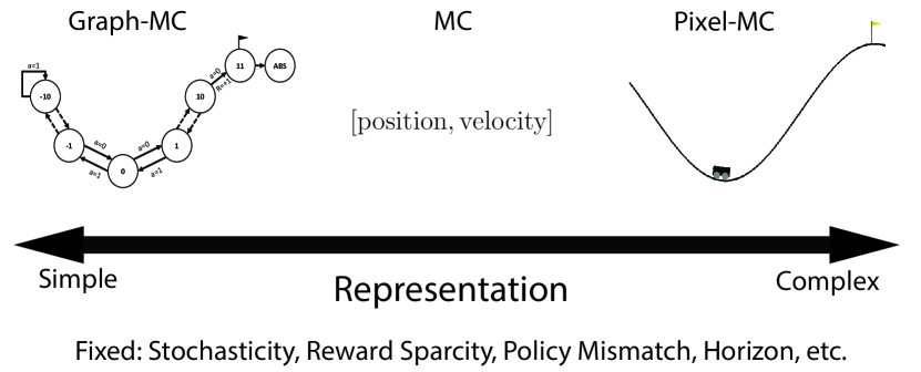
Ultimately, many of the aforementioned factors are intertwined and their usefulness in evaluating OPE performance cannot be considered in isolation. However, they serve as a valuable guide in our selection of benchmark environments. To that end, our benchmark suite includes eight environments. We use two standard RL benchmarks from OpenAI [5]. As many standard RL benchmarks are fixed and deterministic, we design six additional environments that allow control over different design factors. Figure 1 depicts one such design factor: the representation complexity.

Graph: A flexible discrete environment that can vary in horizon, stochasticity, and sparsity.

Graph-POMDP: An extension of Graph to a POMDP setting, where selected information is omitted from the observations that form the behavior data. This enables controlled study of the effect of insufficient representation power relative to other settings in the Graph domain above.

Gridworld (GW): A gridworld design that offers larger state and action space than the Graph domains, longer horizon, and similarly flexible design choices for other environmental factors. Using some version of gridworld is standard across many RL experiments. Gridworld enables simple integration of various designs, and fast data collection.

Pixel-Gridworld (Pix-GW): A scaled-up domain from Gridworld which enables pixel-based representation of the state space. While such usage is not standard in existing literature, this design offers compelling advantage over many existing standard RL benchmarks. First, this domain enables simple controlled experiments to understand the impact of high-dimensional representation on OPE performance, where the ground truth of various quantities to be estimated is readily obtainable thanks to the access to underlying simpler grid representation. Second, this domain effectively simulates high-dimensional experiments with easily tuned experimental conditions, e.g., degree of stochasticity. This design freedom is not available with many currently standard RL benchmarks.

Mountain Car (MC): A standard control domain, which is known to have challenging credit assignment due to sparsity of the reward. Our benchmark for this standard domains allows for function approximation to vary between a linear model and feed-forward neural network, in order to highlight the effects of model misspecification.

Pixel Mountain Car (Pix-MC): A modified version of Mountain Car where the state input is pixel-based, testing the methods’ ability to work in high dimensional settings.

Tabular Mountain Car (Graph-MC) A simplified version of Mountain Car to a graph, allowing us to complete the test for model misspecification by considering the tabular case.

Atari (Enduro) A pixel-based Atari domain. Note that all Atari environments are deterministic and high-dimensional. Instead of choosing many different Atari domains to study, we instead opt to select Enduro as the representative Atari environment, due to its sparsity of reward (and commonly regarded as a highly challenging task). All Atari environments share similar interaction protocol, and can be seamlessly integrated into COBS, if desired.

All together, our benchmark consists of 8 environments with characteristics summarized in Table 1. Complete descriptions can be found in Appendix F. All environments have finite action spaces.

Table 1: Environment characteristics

Environment	Graph	Graph-MC	MC	Pix-MC	Enduro	G-POMDP	GW	Pix-GW
Is MDP?	yes	yes	yes	yes	yes	no	yes	yes
State desc.	pos.	pos.	[pos, vel]	pixels	pixels	pos.	pos.	pixels
$T$	4 or 16	250	250	250	1000	2 or 8	25	25
Stoch Env?	variable	no	no	no	no	no	no	variable
Stoch Rew?	variable	no	no	no	no	no	no	no
Sparse Rew?	variable	terminal	terminal	terminal	dense	terminal	dense	dense
$\hat{Q}$ Class	tabular	tabular	linear/NN	NN	NN	tabular	tabular	NN
Initial state	0	0	variable	variable	gray img	0	variable	variable
Absorb. state	2T	22	[.5,0]	img([.5,0])	zero img	2T	64	zero img
Frame height	1	1	2	2	4	1	1	1
Frame skip	1	1	5	5	1	1	1	1

2.3 Experiment Protocol

Selection of Policies. We use two classes of policies. The first is state-independent with some probability of taking any available action. For example, in the Graph environment with two actions, $\pi(a=0)=p,\pi(a=1)=1-p$ where $p$ is a parameter we can control. The second is a state-dependent $\epsilon-$Greedy policy. We train a policy $Q^{\ast}$ (using value iteration or DDQN [22]) and then vary the deviation away from the policy. Hence $\epsilon-Greedy(Q^{\ast})$ implies we follow a mixed policy $\pi=\operatorname*{arg\,max}_{a}Q^{\ast}(x,a)$ with probability $1-\epsilon$ and uniform with probability $\epsilon$. Here $\epsilon$ is a parameter we can control.

Most OPE methods explicitly require absolute continuity among the policies ($\pi_{b}>0$ whenever $\pi_{e}>0$). Thus, all policies will remain stochastic with this property maintained.

Data Generation & Metrics. Each experiment depends on specifying an environment and its properties, behavior policy $\pi_{b}$, evaluation policy $\pi_{e}$, and number of trajectories $N$ from rolling-out $\pi_{b}$ for historical data. The true on-policy value $V(\pi_{e})$ is the Monte-Carlo estimate via $10,000$ rollouts of $\pi_{e}$. We repeat each experiment $m=10$ times with different random seeds. We judge the quality of a method via two metrics:

• Relative mean squared error (Relative MSE): $\frac{1}{m}\sum_{i=1}^{m}\frac{(\widehat{V}(\pi_{e})_{i}-\frac{1}{m}\sum_{j=1}^{m}V(\pi_{e})_{j})^{2}}{(\frac{1}{m}\sum_{j=1}^{m}V(\pi_{e})_{j})^{2}}$, which allows a fair comparison across different conditions.

• Near-top Frequency: For each experimental condition, we include the number of times each method is within $10\%$ of the best performing one to facilitate aggregate comparison across domains.

Implementation & Hyperparameters. COBS allows running experiments at scale and easy integration with new domains and techniques for future research. The package consists of many domains and reference implementations of OPE methods.

Hyperparameters are selected based on publication, code release or author consultation. We maintain a consistent set of hyperparameters for each estimator and each environment across experimental conditions (see hyperparameter choice in appendix Table G.5).

2.4 Baselines

OPE methods were historically categorized into importance sampling methods, direct methods, or doubly robust methods. This demarcation was first introduced for contextual bandits [15], and later extended to the RL setting [26]. Some recent methods have blurred the boundary of these categories. Examples include Retrace($\lambda$) [37] that uses a product of importance weights of multiple time steps for off-policy $Q$ correction, and MAGIC [51] that switches between importance weighting and direct methods. In this benchmark, we propose to group OPE into three similar classes of methods, but with expanded definition for each category: Inverse Propensity Scoring, Direct Methods, and Hybrid Methods. For the current benchmark, we select representative established baselines from each category. Appendix E contains a full description of all methods under consideration.

Inverse Propensity Scoring (IPS) We consider the main four variants: Importance Sampling (IS), Per-Decision Importance Sampling (PDIS), Weighted Importance Sampling (WIS) and Per-Decision WIS (PDWIS). IPS has a rich history in statistics [44, 20, 24], with successful crossover to RL [45]. The key idea is to reweight the rewards in the historical data by the importance sampling ratio between $\pi_{e}$ and $\pi_{b}$, i.e., how likely a reward is under $\pi_{e}$ versus $\pi_{b}$.

Direct Methods (DM) While some direct methods make use of importance weight adjustments, a key distinction of direct methods is the focus on regression-based techniques to (more) directly estimate the value functions of the evaluation policy ($Q^{\pi_{e}}$ or $V^{\pi_{e}}$). This is an area of very active research with rapidly growing literature. We consider 8 different direct approaches, taken from the following respective families of direct estimators:

Model-based estimators Perhaps the most commonly used DM is Model-based (also called approximate model, denoted AM), where the transition dynamics, reward function and termination condition are directly estimated from historical data [26, 43]. The resulting learned MDP is then used to compute the value of $\pi_{e}$, e.g., by Monte-Carlo policy evaluation. There are also some recent variants of the model-based estimator, e.g., [60].

Value-based estimators Fitted Q Evaluation (FQE) is a model-free counterpart to AM, and is functionally a policy evaluation counterpart to batch Q learning [30]. $\mathbf{Q^{\pi}(\lambda)}$ & Retrace($\mathbf{\lambda}$) & Tree-Backup($\mathbf{\lambda}$) Several model-free methods originated from off-policy learning settings, but are also natural for OPE. $Q^{\pi}(\lambda)$ [21] can be viewed as a generalization of FQE that looks to the horizon limit to incorporate the long-term value into the backup step. Retrace($\lambda$) [37] and Tree-Backup($\lambda$) [45] also use full trajectories, but additionally incorporate varying levels of clipped importance weights adjustment. The $\lambda$-dependent term mitigates instability in the backup step, and is selected based on experimental findings of [37].

Regression-based estimators Direct Q Regression (Q-Reg) & More Robust Doubly-Robust (MRDR) [16] propose two direct methods that make use of cumulative importance weights in deriving the regression estimate for $Q^{\pi_{e}}$, solved through a quadratic program. MRDR changes the objective of the regression to that of directly minimizing the variance of the Doubly-Robust estimator.

Minimax-style estimators [33] recently proposed a method for the infinite horizon setting - we refer to this estimator as IH. While IH can be viewed as a Rao-Blackwellization of the IS estimator, we include it in the DM category because it solves the Bellman equation for state distributions and requires function approximation, which are more characteristic of DM. IH shifts the focus from importance sampling over action sequences to importance ratio between state density distributions induced by $\pi_{b}$ and $\pi_{e}$. Starting with IH, this style of minimax estimator has recently attracted significant attention in OPE literature, including state-action extension of IH [54, 25] and DICE family of estimators [40, 61, 59, 10]. For our benchmarking purpose, we choose IH as the representative of this family.

Hybrid Methods (HM) Hybrid methods subsume doubly robust-like approaches, which combine aspects of both IPS and DM. Standard doubly robust OPE (denoted DR) [26] is an unbiased estimator that leverages DM to decrease the variance of the unbiased estimates produced by importance sampling techniques: Other HM include Weighted Doubly-Robust (WDR) and MAGIC. WDR replaces the importance weights with self-normalized importance weights (similar to WIS). MAGIC introduces adaptive switching between DR and DM; in particular, one can imagine using DR to estimate the value for part of a trajectory and then using DM for the remainder. Using this idea, MAGIC [51] finds an optimal linear combination among a set that varies the switch point between WDR and DM. Note that any DM that returns $\widehat{Q}^{\pi_{e}}(x,a;\theta)$ yields a set of corresponding DR, WDR, and MAGIC estimators. As a result, we consider $21$ hybrid approaches in our experiments.

3 Empirical Evaluation

We evaluate $33$ different OPE methods by running thousands of experiments across the $8$ domains. Due to limited space, we show only the results from selected environmental conditions in the next section. The full detailed results, with highlighted best method in each class, are available in the appendix. The goal of the evaluation is to demonstrate the flexibility of the benchmark suite to systematically test the different factors of influence. We synthesize the results, and then present further considerations and directions for research in Section 4.

3.1 What is the best method?

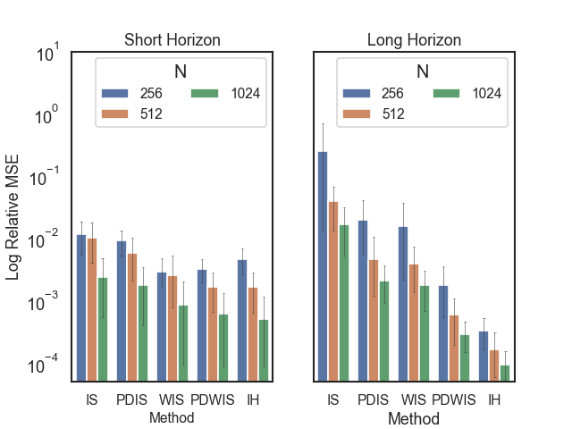
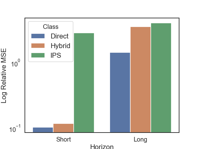
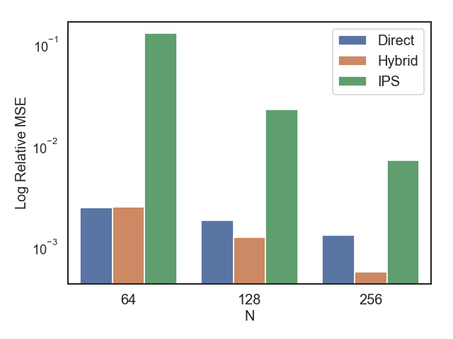
The first important takeaway is that there is no clear-cut winner: no single method or method class is consistently the best performer, as multiple environmental factors can influence the accuracy of each estimator. With that caveat in mind, based on the aggregate top performance metrics, we can recommend from our selected methods the following for each method class (See Figure 3 right, appendix Table D, and appendix Table B).

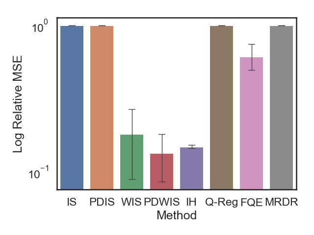
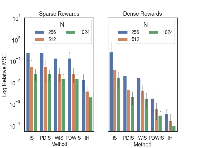
Inverse propensity scoring (IPS). In practice, weighted importance sampling, which is biased, tends to be more accurate and data-efficient than unbiased basic importance sampling methods. Among the four IPS-based estimators, PDWIS tends to perform best (Figure 3 left).

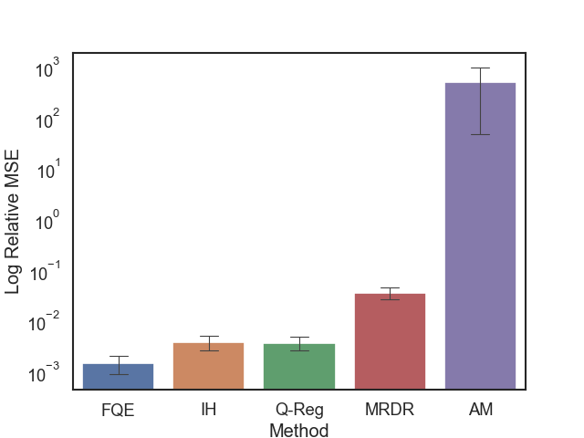
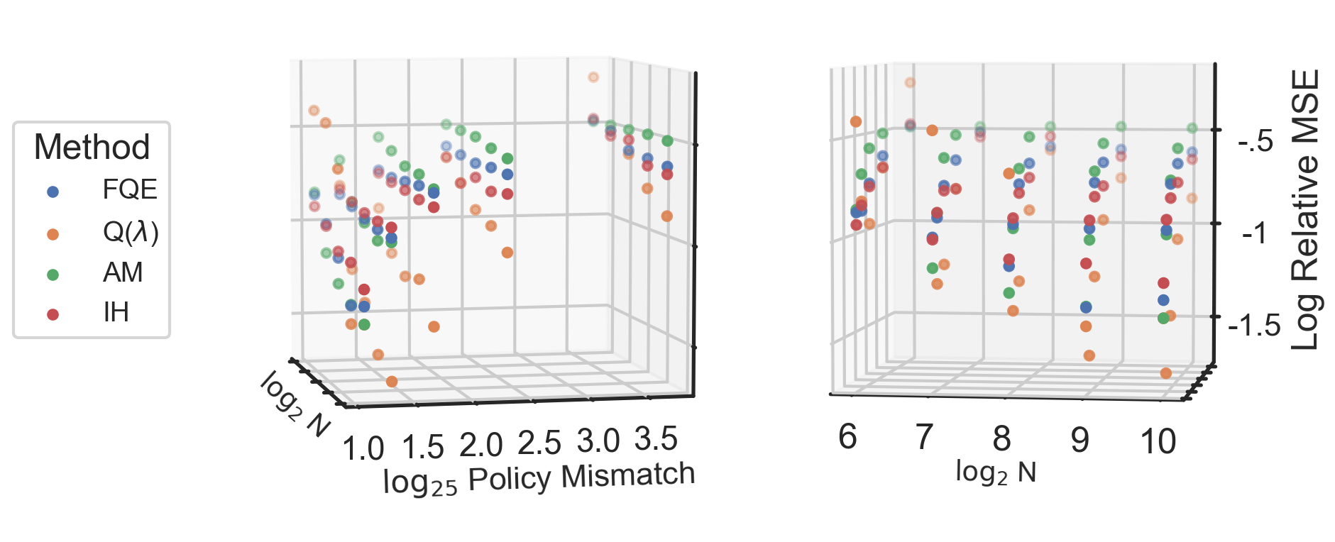
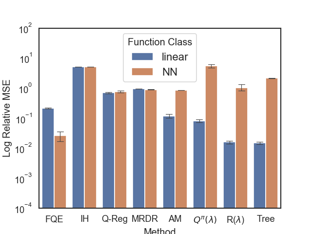
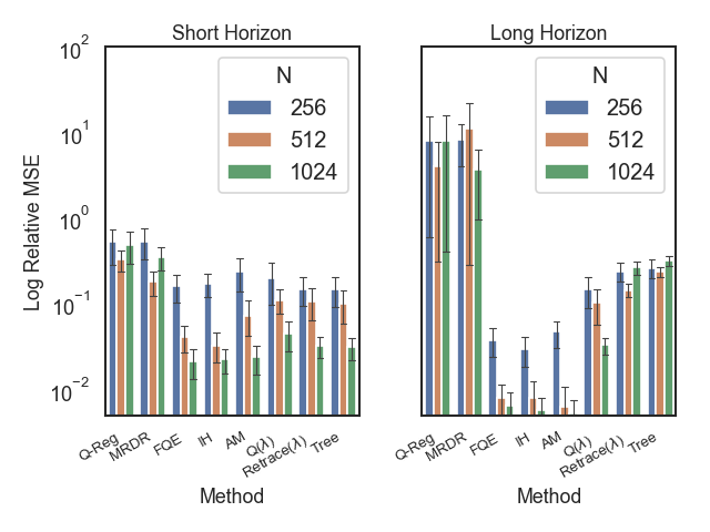
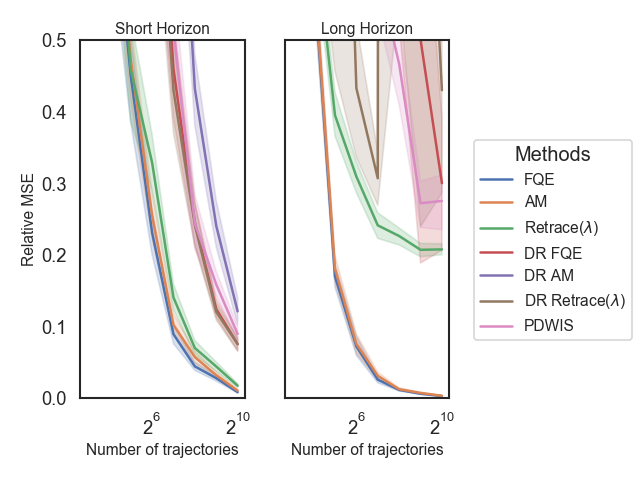
Direct methods (DM). Generally, FQE, $Q^{\pi}(\lambda)$, and IH tend to perform the best among DM (appendix Table B). FQE tends to be more data efficient and is the best method when data is limited (Figure 5). $Q^{\pi}(\lambda)$ generalizes FQE to multi-step backup, and works particularly well with more data, but is computationally expensive in complex domains. IH is highly competitive in long horizons and with high policy mismatch in a tabular setting (appendix Tables B.1, B.1). In pixel-based domains, however, choosing a good kernel function for IH is not straightforward, and IH can underperform other DM (appendix Table B.1). We provide a numerical comparison among direct methods for tabular (appendix Figure H) and complex settings (Figure 3 center).

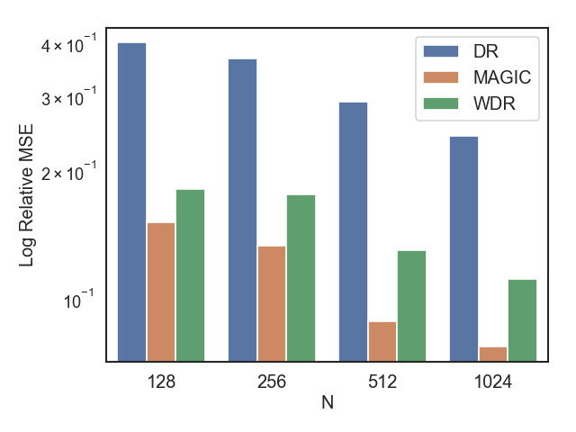
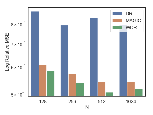
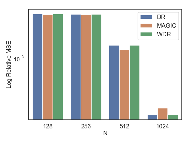
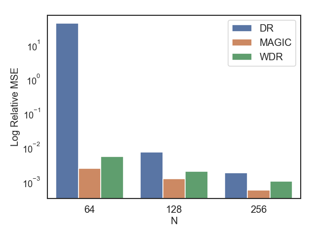
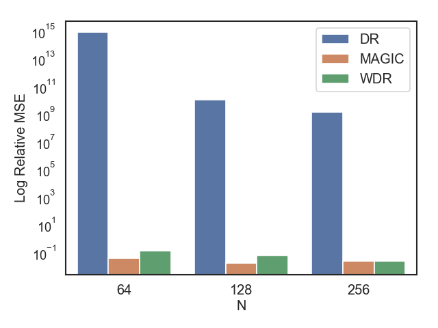
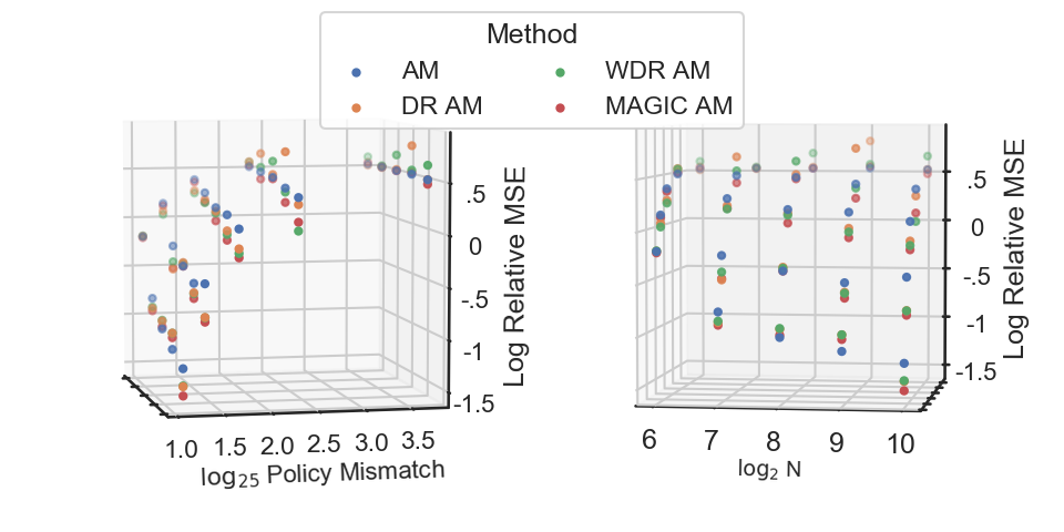
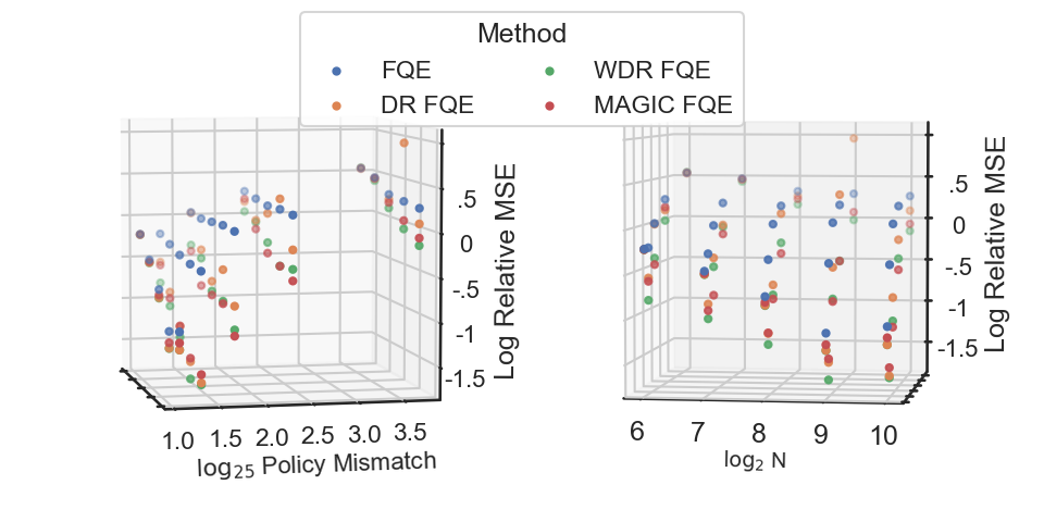
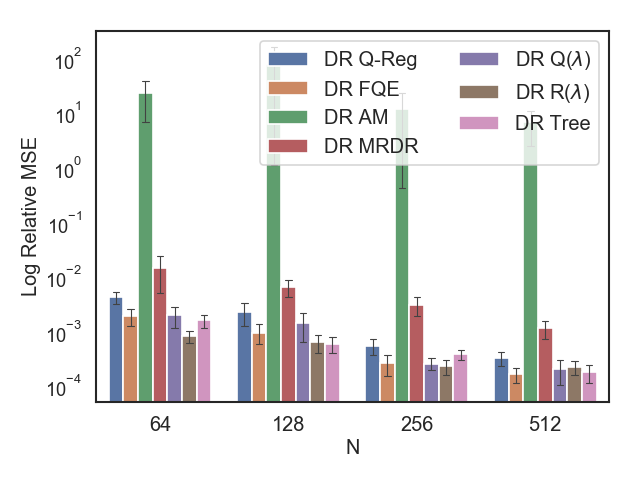
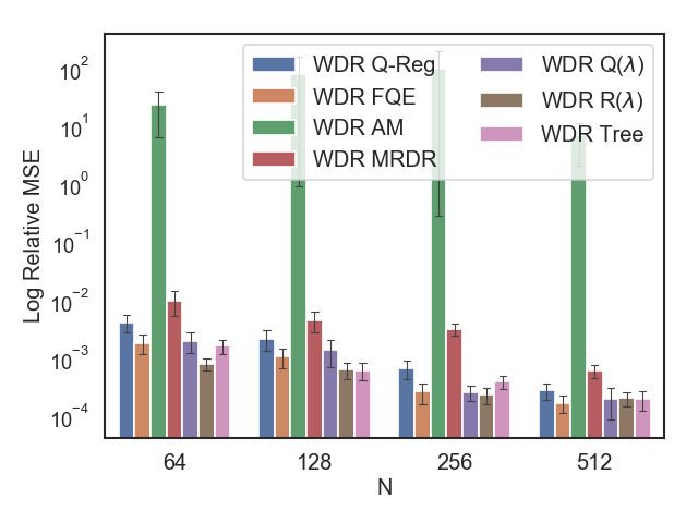
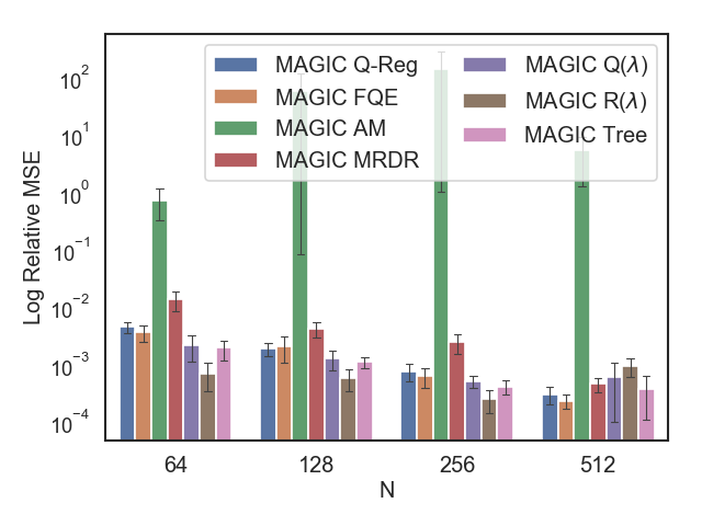
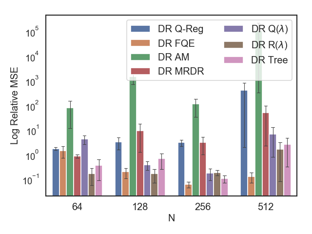
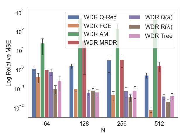
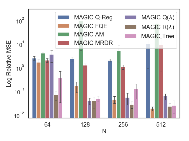
Hybrid methods (HM). With the exception of IH, each DM corresponds to three HM: standard doubly robust (DR), weighted doubly robust (WDR), and MAGIC. For each DM, its WDR version often outperforms its DR version. MAGIC can often outperform WDR and DR. However, MAGIC comes with additional hyperparameters, as one needs to specify the set of partial trajectory length to be considered. Unsurprisingly, their performance highly depends on the underlying DM. In our experiments, FQE and $Q^{\pi}(\lambda)$ are typically the most reliable: MAGIC with FQE or MAGIC with $Q^{\pi}(\lambda)$ tend to be among the best hybrid methods (see appendix Figures H - H).

Figure 2: General Guideline Decision Tree.

3.2 A recipe for method selection

Figure 2 summarizes our general guideline for navigating key factors that affect the accuracy of different estimators. To guide the readers through the process, we now dive further into our experimental design to test various factors, and discuss the resulting insights.

Do we potentially have representation mismatch? Representation mismatch comes from two sources: model misspecification and poor generalization. Model misspecification refers to the insufficient representation power of the function class used to approximate either the transition dynamics (AM), value function (other DM), or state distribution density ratio (in IH).

Having a tabular representation controls for representation mismatch by ensuring adequate function class capacity, as well as zero inherent Bellman error (left branch, Fig 2). In such cases, we may still suffer from poor generalization without sufficient data coverage, which depends on other factors in the domain settings.

The effect of representation mismatch (right branch, Fig 2) can be understood via two scenarios:

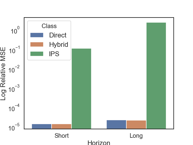
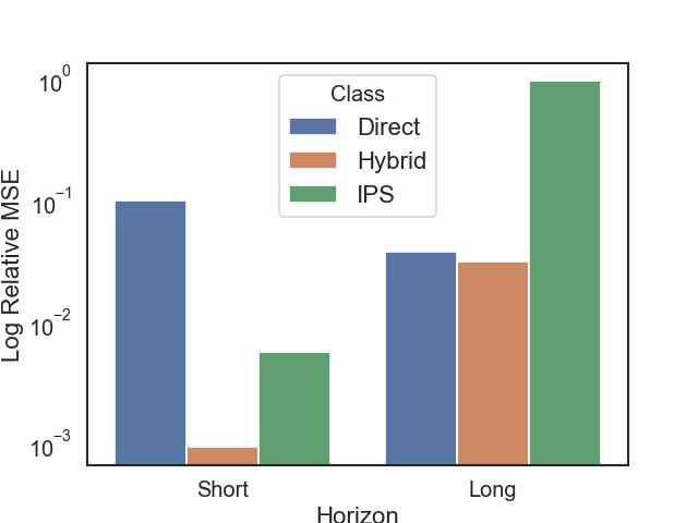
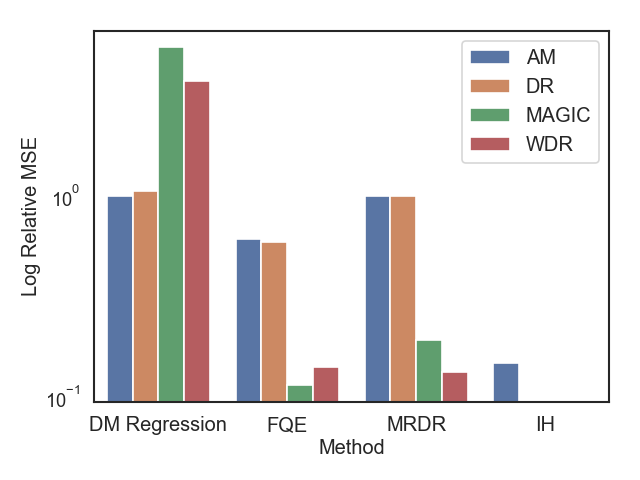
• Misspecified and poor generalization: We expose the impact of this severe mismatch scenario via the Graph POMDP construction, where selected information are omitted from an otherwise equivalent Graph MDP. Here, HM substantially outperforms DM (Figure 4 right versus left).

• Misspecified but good generalization: Function classes such as neural networks have powerful generalization ability, but may introduce bias and inherent Bellman error [38, 9] (see linear vs. neural networks comparison for Mountain Car in appendix Fig H). Still, powerful function approximation makes (biased) DM very competitive with HM, especially under limited data and in complex domains (see pixel-Gridworld in appendix Fig H-H). However, function approximation bias may cause serious problems for high dimensional and long horizon settings. In the extreme case of Enduro (very long horizon and sparse rewards), all DM fail to convincingly outperform a naïve average of behavior data (appendix Fig H).

Method	Near-top Freq.
MAGIC FQE	30.0%
DM FQE	23.7%
IH	19.0%
WDR FQE	17.8%
MAGIC $Q^{\pi}(\lambda)$	17.3%

Figure 3: Left: (Graph domain) Comparing IPS (and IH) under short and long horizon. Mild policy mismatch setting. PDWIS is often best among IPS. But IH outperforms in long horizon. Center: (Pixel-MC) Comparing direct methods in high-dimensional, long horizon setting. Relatively large policy mismatch. FQE and IH tend to outperform. AM is significantly worse in complex domains. Retrace($\lambda$), Q($\lambda$) and Tree-Backup($\lambda$) are very computationally expensive and thus excluded. Right: (Top Methods) The top 5 methods which perform the best across all conditions and domains.

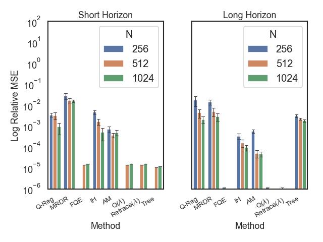
Short horizon vs. Long horizon? It is well-known that IPS methods are sensitive to trajectory length [32]. Long horizon leads to an exponential blow-up of the importance sampling term, and is exacerbated by significant mismatch between $\pi_{b}$ and $\pi_{e}$. This issue is inevitable for any unbiased estimator [26] (a.k.a., the curse of horizon [33]). Similar to IPS, DM relying on importance weights also suffer in long horizons (appendix Fig H), though to a lesser degree. IH aims to bypass the effect of cumulative weighting in long horizons, and indeed performs substantially better than IPS methods in very long horizon domains (Fig 3 left).

A frequently ignored aspect in previous OPE work is a proper distinction between fixed, finite horizon tasks (IPS focus), infinite horizon tasks (IH focus), and indefinite horizon tasks, where the trajectory length is finite but varies depending on the policy. Many applications should properly belong to the indefinite horizon category. Applying HM in this setting requires proper padding of the rewards (without altering the value function in the infinite horizon limit) as DR correction typically assumes fixed length trajectories.

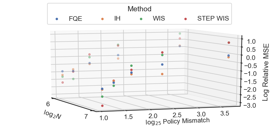
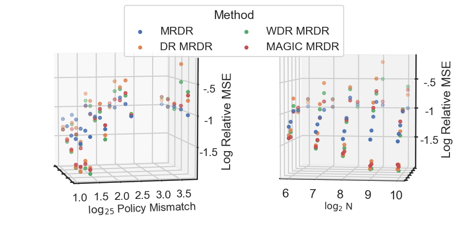
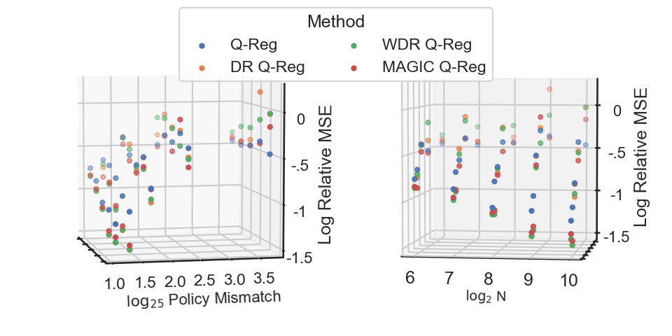
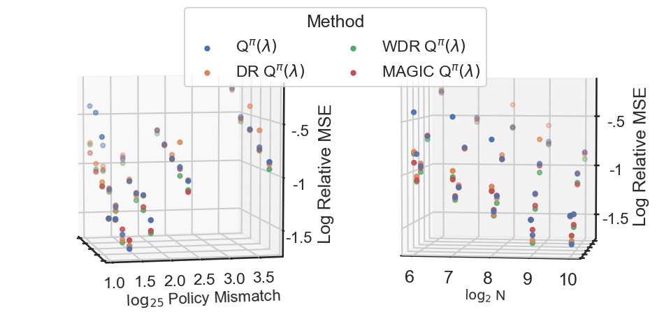
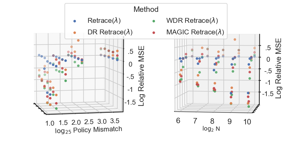
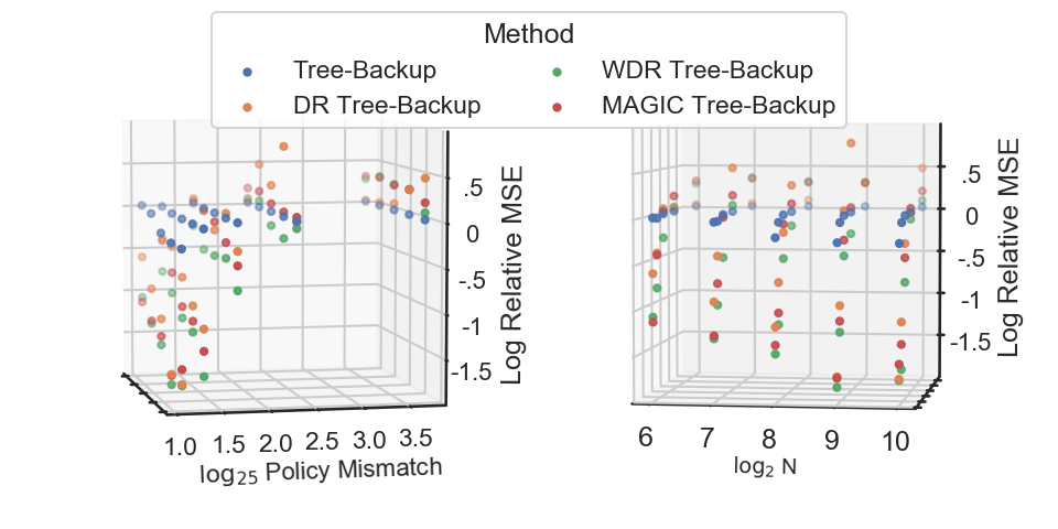
How different are behavior and target policies? Similar to IPS, the performance of DM is negatively correlated with the degree of policy mismatch. Figure 5 shows the interplay of increasing policy mismatch and historical data size, on the top DM in the deterministic gridworld. We use $(\sup_{a\in A,x\in X}{\frac{\pi_{e}(a|x)}{\pi_{b}(a|x)}})^{T}$ as an environment-independent metric of mismatch between the two policies. The performance of the top DM (FQE, $Q^{\pi}(\lambda)$, IH) tend to hold up better than IPS methods when the policy gap increases (appendix Figure H). FQE and IH are best in the small data regime, and $Q^{\pi}(\lambda)$ performs better as data size increases (Figure 5). Increased policy mismatch weakens the DM that use importance weights (Q-Reg, MRDR, Retrace($\lambda$) and Tree-Backup($\lambda$)).

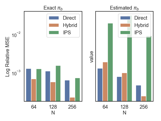
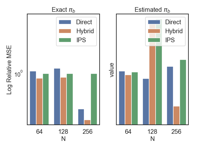
Do we have a good estimate of the behavior policy? Often the behavior policy may not be known exactly and requires estimation, which can introduce bias and cause HM to underperform DM, especially in low data regime (e.g., pixel gridworld appendix Figure H-H). Similar phenomenon was observed in the statistics literature [29]. As the data size increases, HMs regain the advantage as the quality of the $\pi_{b}$ estimate improves.

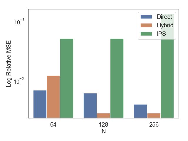
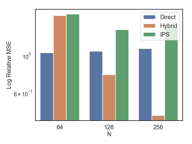
Is the environment stochastic or deterministic? While stochasticity affects all methods by straining the data requirement, HM are more negatively impacted than DM (Figure 4 center, Figure H). This can be justified by e.g., the variance analysis of DR, which shows that the variance of the value function with respect to stochastic transitions will be amplified by cumulative importance weights and then contribute to the overall variance of the estimator; see [26, Theorem 1] for further details. We empirically observe that DM frequently outperform their DR versions in the small data case (Figure H). In a stochastic environment and tabular setting, HM do not provide significant edge over DM, even in short horizon case. The gap closes as the data size increases (Figure H).

Figure 4: Comparing IPS versus Direct methods versus Hybrid methods under short and long horizon, large policy mismatch and large data. Left: (Graph domain) Deterministic environment. Center: (Graph domain) Stochastic environment and rewards. Right: (Graph-POMDP) Model misspecification (POMDP). Minimum error per class is shown.

Figure 5: (Gridworld domain) Errors are directly correlated with policy mismatch but inversely correlated with data size. We pick the best direct methods for illustration. The two plots represent the same figure from two different vantage points.

3.3 Challenging common wisdom

To illustrate the value of a flexible benchmarking tool, in this section we further synthesize the empirical findings and stress-test several commonly held beliefs about the high-level performance of OPE methods.

Is HM always better than DM? No. Overall, DM are surprisingly competitive with HM. Under high-dimensionality, long horizons, estimated behavior policies, or reward/environment stochasticity, HM can underperform simple DM, sometimes significantly (e.g., see appendix Figure H).

Concretely, HM can perform worse than DM in the following scenarios that we tested:

• Tabular with large policy mismatch, or stochastic environments (appendix Figure H, Table B.1, B.1).

• Complex domains with long horizon and unknown behavior policy (app. Figure H-H, Table B.1).

When data is sufficient, or model misspecification is severe, HM provides consistent gains over DM.

Is horizon length the most important factor? No. Despite conventional wisdom suggesting IPS methods are most sensitive to horizon length, we find that this is not always the case. Policy divergence $\sup_{a\in A,x\in X}\frac{\pi_{e}(a|x)}{\pi_{b}(a|x)}$ can be just as, if not more, meaningful. For comparison, we designed two scenarios with identical mismatch $(\sup_{a\in A,x\in X}\frac{\pi_{e}(a|x)}{\pi_{b}(a|x)})^{T}$ as defined in Section 3.2 (see appendix Tables C, C). Starting from a baseline scenario of short horizon and small policy divergence (appendix Table C), extending horizon length leads to $10\times$ degradation in accuracy, while a comparable increase in policy divergence causes a $100\times$ degradation.

How good is model-based direct method (AM)? AM can be among the worst performing direct methods (appendix Table B). While AM performs well in tabular setting in the large data case (appendix Figure H), it tends to perform poorly in high dimensional settings with function approximation (e.g., Figure 3 center). Fitting the transition model $P(x^{\prime}|x,a)$ is often more prone to small errors than directly approximating $Q(x,a)$. Model fitting errors also compound with long horizons.

4 Discussion and Future Directions

Finally, we close with a brief discussion on some limitations common to recent OPE benchmarks and more generally OPE experimental studies, and point to areas of development for future studies.

Lack of short-horizon benchmark in high-dimensional settings. Evaluation of other complex RL tasks with short horizon is currently beyond the scope of our study, due to the lack of a natural benchmark. For contextual bandits, it has been shown that while DR is highly competitive, it is sometimes substantially outperformed by DM [56]. New benchmark tasks should have longer horizon than contextual bandits, but shorter than typical Atari games. We also currently lack natural stochastic environments in high-dimensional RL benchmarks. An example candidate for medium horizon, complex OPE domain is NLP tasks such as dialogue.

Other OPE settings. We outline practically relevant settings that can benefit from benchmarking:

• Missing data coverage. A common assumption in the analysis of OPE is a full support assumption: $\pi_{e}(a|x)>0$ implies $\pi_{b}(a|x)>0$, which often ensure unbiasedness of estimators [45, 33, 15]. This assumption is often not verifiable in practice. Practically, violation of this assumption requires regularization of unbiased estimators to avoid ill-conditioning [33, 16]. One avenue to investigate is to optimize the bias-variance trade-off when the full support is not applicable.

• Confounding variables. Existing OPE research often assumes that the behavior policy chooses actions solely based on the state. This assumption is often violated when the decisions in the historical data are made by humans instead of algorithms, who may base their decisions on variables not recorded in the data, causing confounding effects. Tackling this challenge, possibly using techniques from causal inference [50, 42], is an important future direction.

• Strategic Environmental Behavior. Most OPE methods have focused exclusively on single-agent scenarios under well-defined MDP. Realitic applications of offline RL may have to deal with nonstationary and partial observability induced by strategic behavior from multiple agents [62]. There is currently a lack of a compelling domain to study such a setting.

Evaluating new OPE estimators. For our empirical evaluation, we selected a representative set of established baseline approaches from multiple OPE method families. Currently this area of research is very active and as such, new OPE estimators have been and will continue to be proposed. We discuss several new minimax style estimators, notably the DICE family in section 2.4. A minimax-style estimator has also been recently proposed for the model-based regime [55]. Among the ideas that use marginalized state distribution [58] to improve over standard IPS, [27, 28] analyze double reinforcement learning estimator that makes use of both estimates for $Q$ function and state density ratio. While we have not included all estimators in our current benchmark, our software implementation is highly modular and can easily accommodate new estimators and environments.

Algorithmic approach to method selection. Using COBS, we showed how to distill a general guideline for selecting OPE methods. However, it is often not easy to judge whether some decision criteria are satisfied (e.g., quantifying model misspecification, degree of stochasticity, or appropriate data size). As more OPE methods continue to be developed, an important missing piece is a systematic technique for model selection, given a relatively high degree of variability among existing techniques.

Appendix A Glossary of Terms

See Table A for a description of the terms used in this paper.

Table 2: Glossary of terms

Acronym	Term
OPE	Off-Policy Policy Evaluation
$X$	State Space
$A$	Action Space
$P$	Transition Function
$R$	Reward Function
$\gamma$	Discount Factor
$d_{0}$	Initial State Distribution
$D$	Dataset
$\tau$	Trajectory/Episode
$T$	Horizon/Episode Length
$N$	Number of episodes in $D$
$\pi_{b}$	Behavior Policy
$\pi_{e}$	Evaluation Policy
$V$	Value, ex: $V(x)$
$Q$	Action-Value, ex: $Q(x,a)$
$\rho_{j:j^{\prime}}^{i}$	Cumulative Importance Weight, $\prod_{t=j}^{\min(j^{\prime},T-1)}\frac{\pi_{e}(a_{t}^{i}|x_{t}^{i})}{\pi_{b}(a_{t}^{i}|x_{t}^{i})}$. If $j>j^{\prime}$ then default is $\rho=1$
IPS	Inverse Propensity Scoring
DM	Direct Method
HM	Hybrid Method
IS	Importance Sampling
PDIS	Per-Decision Importance Sampling
WIS	Weighted Importance Sampling
PDWIS	Per-Decision Weighted Importance Sampling
FQE	Fitted Q Evaluation [30]
IH	Infinite Horizon [33]
Q-Reg	Q Regression [16]
MRDR	More Robust Doubly Robst [16]
AM	Approximate Model (Model Based)
$Q(\lambda)$	$Q^{\pi}(\lambda)$ [21]
$R(\lambda)$	Retrace$(\lambda)$ [37]
Tree	Tree-Backup$(\lambda)$ [45]
DR	Doubly-Robust [26, 15]
WDR	Weighted Doubly-Robust [15]
MAGIC	Model And Guided Importance Sampling Combining (Estimator) [51]
Graph	Graph Environment
Graph-MC	Graph Mountain Car Environment
MC	Mountain Car Environment
Pix-MC	Pixel-Based Mountain Car Environment
Enduro	Enduro Environment
Graph-POMDP	Graph-POMDP Environment
GW	Gridworld Environment
Pix-GW	Pixel-Based Gridworld Environment

Appendix B Ranking of Methods

A method that is within $10\%$ of the method with the lowest Relative MSE is counted as a top method, called Near-top Frequency, and then we aggregate across all experiments. See Table B for a sorted list of how often the methods appear within $10\%$ of the best method.

Table 3: Fraction of time among the top estimators across all experiments

Method	Near-top Frequency
MAGIC FQE	0.300211
DM FQE	0.236786
IH	0.190275
WDR FQE	0.177590
MAGIC $Q^{\pi}(\lambda)$	0.173362
WDR $Q^{\pi}(\lambda)$	0.173362
DM $Q^{\pi}(\lambda)$	0.150106
DR $Q^{\pi}(\lambda)$	0.135307
WDR R($\lambda$)	0.133192
DR FQE	0.128964
MAGIC R($\lambda$)	0.107822
WDR Tree	0.105708
DR R($\lambda$)	0.105708
DM R($\lambda$)	0.097252
DM Tree	0.084567
MAGIC Tree	0.076110
DR Tree	0.073996
DR MRDR	0.073996
WDR Q-Reg	0.071882
DM AM	0.065539
IS	0.063425
WDR MRDR	0.054968
PDWIS	0.046512
DR Q-Reg	0.044397
MAGIC AM	0.038055
MAGIC MRDR	0.033827
DM MRDR	0.033827
PDIS	0.033827
MAGIC Q-Reg	0.027484
WIS	0.025370
NAIVE	0.025370
DM Q-Reg	0.019027
DR AM	0.012685
WDR AM	0.006342

B.1 Decision Tree Support

Tables B.1-B.1 provide a numerical support for the decision tree in the main paper (Figure 2). Each table refers to a child node in the decision tree, ordered from left to right, respectively. For example, Table B.1 refers to the left-most child node (propery specified, short horizon, small policy mismatch) while Table B.1 refers to the right-most child node (misspecified, good representation, long horizon, good $\pi_{b}$ estimate).

Table 4: Near-top Frequency among the properly specified, short horizon, small policy mismatch experiments

	DM	Hybrid
	Direct	DR	WDR	MAGIC
AM	4.7%	4.7%	3.1%	4.7%
Q-Reg	0.0%	4.7%	6.2%	4.7%
MRDR	7.8%	14.1%	7.8%	7.8%
FQE	40.6%	23.4%	21.9%	34.4%
R$(\lambda)$	17.2%	20.3%	20.3%	14.1%
Q${}^{\pi}(\lambda)$	21.9%	18.8%	18.8%	17.2%
Tree	15.6%	12.5%	12.5%	14.1%
IH	17.2%	-	-	-

	IPS
	Standard	Per-Decision
IS	4.7%	4.7%
WIS	3.1%	3.1%
NAIVE	1.6%	-

Table 5: Near-top Frequency among the properly specified, short horizon, large policy mismatch experiments

	DM	Hybrid
	Direct	DR	WDR	MAGIC
AM	20.3%	1.6%	0.0%	7.8%
Q-Reg	1.6%	1.6%	3.1%	1.6%
MRDR	3.1%	1.6%	6.2%	1.6%
FQE	35.9%	14.1%	17.2%	37.5%
R$(\lambda)$	23.4%	14.1%	20.3%	23.4%
Q${}^{\pi}(\lambda)$	15.6%	15.6%	14.1%	20.3%
Tree	21.9%	12.5%	18.8%	21.9%
IH	29.7%	-	-	-

	IPS
	Standard	Per-Decision
IS	0.0%	0.0%
WIS	0.0%	1.6%
NAIVE	3.1%	-

Table 6: Near-top Frequency among the properly specified, long horizon, small policy mismatch experiments

	DM	Hybrid
	Direct	DR	WDR	MAGIC
AM	6.9%	0.0%	0.0%	5.6%
Q-Reg	0.0%	1.4%	1.4%	1.4%
MRDR	1.4%	0.0%	1.4%	2.8%
FQE	50.0%	22.2%	23.6%	50.0%
R$(\lambda)$	13.9%	12.5%	11.1%	9.7%
Q${}^{\pi}(\lambda)$	20.8%	18.1%	18.1%	18.1%
Tree	2.8%	1.4%	0.0%	2.8%
IH	29.2%	-	-	-

	IPS
	Standard	Per-Decision
IS	0.0%	0.0%
WIS	0.0%	0.0%
NAIVE	5.6%	-

Table 7: Near-top Frequency among the properly specified, long horizon, large policy mismatch, deterministic env/rew experiments

	DM	Hybrid
	Direct	DR	WDR	MAGIC
AM	3.5%	3.5%	1.8%	1.8%
Q-Reg	3.5%	1.8%	0.0%	0.0%
MRDR	3.5%	1.8%	0.0%	0.0%
FQE	15.8%	17.5%	29.8%	28.1%
R$(\lambda)$	1.8%	3.5%	0.0%	0.0%
Q${}^{\pi}(\lambda)$	22.8%	15.8%	38.6%	24.6%
Tree	3.5%	3.5%	1.8%	1.8%
IH	21.1%	-	-	-

	IPS
	Standard	Per-Decision
IS	5.3%	3.5%
WIS	0.0%	8.8%
NAIVE	0.0%	-

Table 8: Near-top Frequency among the properly specified, long horizon, large policy mismatch, stochastic env/rew experiments

	DM	Hybrid
	Direct	DR	WDR	MAGIC
AM	14.6%	0.0%	0.0%	8.3%
Q-Reg	4.2%	2.1%	0.0%	2.1%
MRDR	4.2%	2.1%	0.0%	0.0%
FQE	31.2%	2.1%	0.0%	25.0%
R$(\lambda)$	4.2%	6.2%	0.0%	0.0%
Q${}^{\pi}(\lambda)$	2.1%	0.0%	0.0%	2.1%
Tree	4.2%	6.2%	0.0%	0.0%
IH	41.7%	-	-	-

	IPS
	Standard	Per-Decision
IS	25.0%	4.2%
WIS	0.0%	0.0%
NAIVE	2.1%	-

Table 9: Near-top Frequency among the potentially misspecified, insufficient representation experiments

	DM	Hybrid
	Direct	DR	WDR	MAGIC
AM	-	-	-	-
Q-Reg	3.9%	13.7%	25.5%	6.9%
MRDR	0.0%	18.6%	15.7%	5.9%
FQE	0.0%	5.9%	13.7%	24.5%
R$(\lambda)$	-	-	-	-
Q${}^{\pi}(\lambda)$	-	-	-	-
Tree	-	-	-	-
IH	6.9%	-	-	-

	IPS
	Standard	Per-Decision
IS	10.8%	8.8%
WIS	9.8%	13.7%
NAIVE	3.9%	-

Table 10: Near-top Frequency among the potentially misspecified, sufficient representation, poor $\pi_{b}$ estimate experiments

	DM	Hybrid
	Direct	DR	WDR	MAGIC
AM	0.0%	0.0%	0.0%	0.0%
Q-Reg	0.0%	0.0%	3.3%	0.0%
MRDR	13.3%	6.7%	0.0%	0.0%
FQE	0.0%	3.3%	6.7%	10.0%
R$(\lambda)$	16.7%	0.0%	6.7%	20.0%
Q${}^{\pi}(\lambda)$	6.7%	0.0%	0.0%	3.3%
Tree	20.0%	0.0%	6.7%	6.7%
IH	0.0%	-	-	-

	IPS
	Standard	Per-Decision
IS	3.3%	0.0%
WIS	0.0%	0.0%
NAIVE	0.0%	-

Table 11: Near-top Frequency among the potentially misspecified, sufficient representation, good $\pi_{b}$ estimate experiments

	DM	Hybrid
	Direct	DR	WDR	MAGIC
AM	0.0%	0.0%	0.0%	2.8%
Q-Reg	0.0%	0.0%	0.0%	0.0%
MRDR	0.0%	5.6%	0.0%	5.6%
FQE	8.3%	8.3%	25.0%	11.1%
R$(\lambda)$	2.8%	8.3%	8.3%	19.4%
Q${}^{\pi}(\lambda)$	5.6%	5.6%	8.3%	0.0%
Tree	5.6%	8.3%	16.7%	5.6%
IH	0.0%	-	-	-

	IPS
	Standard	Per-Decision
IS	0.0%	0.0%
WIS	0.0%	0.0%
NAIVE	0.0%	-

Appendix C Supplementary Folklore Backup

The following tables represent the numerical support for how horizon and policy difference affect the performance of the OPE estimators when policy mismatch is held constant. Notice that the policy mismatch for table C and C are identical: $\left(\frac{.124573\ldots}{.1}\right)^{100}=\left(\frac{.9}{.1}\right)^{10}$. What we see here is that despite identical policy mismatch, the longer horizon does not impact the error as much (compared to the baseline, Table C) as moving $\pi_{e}$ to $.9$, far from $.1$ and keeping the horizon the same.

Table 12: Graph, relative MSE. $T=10,N=50,\pi_{b}(a=0)=0.1,\pi_{e}(a=0)=0.1246$. Dense rewards. Baseline.

	DM	Hybrid
	Direct	DR	WDR	MAGIC
AM	1.9E-3	4.9E-3	5.0E-3	3.4E-3
Q-Reg	2.4E-3	4.3E-3	4.2E-3	4.5E-3
MRDR	5.8E-3	8.9E-3	9.4E-3	9.2E-3
FQE	1.8E-3	1.8E-3	1.8E-3	1.8E-3
R$(\lambda)$	1.8E-3	1.8E-3	1.8E-3	1.8E-3
Q${}^{\pi}(\lambda)$	1.8E-3	1.8E-3	1.8E-3	1.8E-3
Tree	1.8E-3	1.8E-3	1.8E-3	1.8E-3
IH	1.6E-3	-	-	-

	IPS
	Standard	Per-Decision
IS	5.6E-4	8.4E-4
WIS	1.4E-3	1.4E-3
NAIVE	6.1E-3	-

Table 13: Graph, relative MSE. $T=100,N=50,\pi_{b}(a=0)=0.1,\pi_{e}(a=0)=0.1246$. Dense rewards. Increasing horizon compared to baseline, fixed $\pi_{e}$.

	DM	Hybrid
	Direct	DR	WDR	MAGIC
AM	5.6E-2	5.9E-2	5.9E-2	5.3E-2
Q-Reg	3.4E-3	1.1E-1	1.2E-1	9.2E-2
MRDR	1.1E-2	2.5E-1	2.9E-1	3.1E-1
FQE	6.0E-2	6.0E-2	6.0E-2	6.0E-2
R$(\lambda)$	6.0E-2	6.0E-2	6.0E-2	6.0E-2
Q${}^{\pi}(\lambda)$	6.0E-2	6.0E-2	6.0E-2	6.0E-2
Tree	3.4E-1	7.0E-3	1.6E-3	2.3E-3
IH	4.7E-4	-	-	-

	IPS
	Standard	Per-Decision
IS	1.7E-2	2.5E-3
WIS	9.5E-4	4.9E-4
NAIVE	5.4E-3	-

Table 14: Graph, relative MSE. $T=10,N=50,\pi_{b}(a=0)=0.1,\pi_{e}(a=0)=0.9$. Dense rewards. Increasing $\pi_{e}$ compared to baseline, fixed horizon.

	DM	Hybrid
	Direct	DR	WDR	MAGIC
AM	6.6E-1	6.7E-1	6.6E-1	6.6E-1
Q-Reg	5.4E-1	6.3E-1	1.3E0	9.3E-1
MRDR	5.4E-1	7.3E-1	2.0E0	2.0E0
FQE	6.6E-1	6.6E-1	6.6E-1	6.6E-1
R$(\lambda)$	6.7E-1	6.6E-1	9.3E-1	1.0E0
Q${}^{\pi}(\lambda)$	6.6E-1	6.6E-1	6.6E-1	6.6E-1
Tree	6.7E-1	6.6E-1	9.4E-1	1.0E0
IH	1.4E-2	-	-	-

	IPS
	Standard	Per-Decision
IS	1.0E0	5.4E-1
WIS	2.0E0	9.7E-1
NAIVE	4.0E0	-

Appendix D Model Selection Guidelines

For the definition of near-top frequency, see the definition in Section 2.3. For support of the guideline, see Table B)

Table 15: Model Selection Guidelines.

Class	Recommendation	When to use	Prototypical env.	Near-top Freq.
Direct	FQE	Stochastic env, severe policy mismatch	Graph, MC, Pix-MC	23.7%
	$Q(\lambda)$	Compute non-issue, moderate policy mismatch	GW/Pix-GW	15.0%
	IH	Long horizon, mild policy mismatch, good kernel	Graph-MC	19.0%
IPS	PDWIS	Short horizon, mild policy mismatch	Graph	4.7%
Hybrid	MAGIC FQE	Severe model misspecification	Graph-POMDP, Enduro	30.0%
	MAGIC $Q(\lambda)$	Compute non-issue, severe model misspecification	Graph-POMDP	17.3%

Appendix E Methods

Below we include a description of each of the methods we tested. Let $\tilde{T}=T-1$.

E.1 Inverse Propensity Scoring (IPS) Methods

Table 16: IPS methods. [15, 26]

	Standard	Per-Decision
IS	$\sum_{i=1}^{N}\frac{\rho^{i}_{0:\tilde{T}}}{N}\sum_{t=0}^{\tilde{T}}\gamma^{t}r_{t}$	$\sum_{i=1}^{N}\sum_{t=0}^{\tilde{T}}\gamma^{t}\frac{\rho^{i}_{0:t}}{N}r_{t}$
WIS	$\sum_{i=1}^{N}\frac{\rho^{i}_{0:\tilde{T}}}{w_{0:\tilde{T}}}\sum_{t=0}^{\tilde{T}}\gamma^{t}r_{t}$	$\sum_{i=1}^{N}\sum_{t=0}^{\tilde{T}}\gamma^{t}\frac{\rho^{i}_{0:t}}{w_{0:t}}r_{t}$

Table E.1 shows the calculation for the four traditional IPS estimators: $V_{IS},V_{PDIS},V_{WIS},V_{PDWIS}$. In addition, we include the following method as well since it is a Rao-Blackwellization [33] of the IPS estimators:

E.2 Hybrid Methods

Hybrid rely on being supplied an action-value function $\widehat{Q}$, an estimate of $Q$, from which one can also yield $\widehat{V}(x)=\sum_{a\in A}\pi(a|x)\widehat{Q}(x,a)$. Doubly-Robust (DR): [51, 26]

$$V_{DR}=\frac{1}{N}\sum_{i=1}^{N}\widehat{V}(x_{0}^{i})+\\ \frac{1}{N}\sum_{i=1}^{N}\sum_{t=0}^{\infty}\gamma^{t}\rho_{0:t}^{i}[r_{t}^{i}-\widehat{Q}(x_{t}^{i},a_{t}^{i})+\gamma\widehat{V}(x_{t+1}^{i})]$$

Weighted Doubly-Robust (WDR): [51]

$$V_{WDR}=\frac{1}{N}\sum_{i=1}^{N}\widehat{V}(x_{0}^{i})+\\ \sum_{i=1}^{N}\sum_{t=0}^{\infty}\gamma^{t}\frac{\rho^{i}_{0:t}}{w_{0:t}}[r_{t}^{i}-\widehat{Q}(x_{t}^{i},a_{t}^{i})+\gamma\widehat{V}(x_{t+1}^{i})]$$

MAGIC: [51] Given $g_{J}=\{g^{i}|i\in J\subseteq\mathbb{N}\cup\{-1\}\}$ where

$$g^{j}(D)=\sum_{i=1}^{N}\sum_{t=0}^{j}\gamma^{t}\frac{\rho^{i}_{0:t}}{w_{0:t}}r_{t}^{i}+\sum_{i=1}^{N}\gamma^{j+1}\frac{\rho^{i}_{0:t}}{w_{0:t}}\widehat{V}(x_{j+1}^{i})-\\ \sum_{i=1}^{N}\sum_{t=0}^{j}\gamma^{t}(\frac{\rho^{i}_{0:t}}{w_{0:t}}\widehat{Q}(x_{t}^{i},a_{t}^{i})-\frac{\rho^{i}_{0:\tilde{T}}}{w_{0:\tilde{T}}}\widehat{V}(x_{t}^{i})),$$

then define $dist(y,Z)=\min_{z\in Z}|y-z|$ and

$$\widehat{b}_{n}(j) =dist(g^{J}_{j}(D),CI(g^{\infty}(D),0.5))$$

$$\widehat{\Omega}_{n}(i,j) =Cov(g^{J}_{i}(D),g^{J}_{j}(D))$$

then, for a $|J|-$simplex $\Delta^{|J|}$ we can calculate

$$\widehat{x}^{\ast}\in\arg\min_{x\in\Delta^{|J|}}x^{T}[\widehat{\Omega}_{n}+\widehat{b}\widehat{b}^{T}]x$$

which, finally, yields

$$V_{MAGIC}=(\widehat{x}^{\ast})^{T}g_{J}.$$

MAGIC can be thought of as a weighted average of different blends of the DM and Hybrid. In particular, for some $i\in J$, $g^{i}$ represents estimating the first $i$ steps of $V(\pi_{e})$ according to DR (or WDR) and then estimating the remaining steps via $\widehat{Q}$. Hence, $V_{MAGIC}$ finds the most appropriate set of weights which trades off between using a direct method and a Hybrid.

E.3 Direct Methods (DM)

E.3.1 Model-Based

Approximate Model (AM): [26] An approach to model-based value estimation is to directly fit the transition dynamics $P(x_{t+1}|x_{t},a_{t})$, reward $R(x_{t},a_{t})$, and terminal condition $P(x_{t+1}\in X_{terminal}|x_{t},a_{t})$ of the MDP using some for of maximum likelihood or function approximation. This yields a simulation environment from which one can extract the value of a policy using an average over rollouts. Thus, $V(\pi)=\mathbb{E}[\sum_{t=1}^{T}\gamma^{t}r(x_{t},a_{t})|x_{0}=x,a_{0}=\pi(x_{0})]$ where the expectation is over initial conditions $x\sim d_{0}$ and the transition dynamics of the simulator.

E.3.2 Model-Free

Every estimator in this section will approximate $Q$ with $\widehat{Q}(\cdot;\theta)$, parametrized by some $\theta$. From $\widehat{Q}$ the OPE estimate we seek is

$$V=\frac{1}{N}\sum_{i=1}^{N}\sum_{a\in A}\pi_{e}(a|s)\widehat{Q}(s_{0}^{i},a;\theta)$$

Note that $\mathbb{E}_{\pi_{e}}Q(x_{t+1},\cdot)=\sum_{a\in A}\pi_{e}(a|x_{t+1})Q(x_{t+1},a)$.

Direct Model Regression (Q-Reg): [16]

$$\widehat{Q}(\cdot,\theta) =\min_{\theta}\frac{1}{N}\sum_{i=1}^{N}\sum_{t=0}^{\tilde{T}}\gamma^{t}\rho_{0:t}^{i}\left(R^{i}_{t:\tilde{T}}-\widehat{Q}(x^{i}_{t},a^{i}_{t};\theta)\right)^{2}$$

$$R^{i}_{t:\tilde{T}} =\sum_{t^{\prime}=t}^{\tilde{T}}\gamma^{t^{\prime}-t}\rho_{(t+1):t^{\prime}}^{i}r^{i}_{t^{\prime}}$$

Fitted Q Evaluation (FQE): [30] $\widehat{Q}(\cdot,\theta)=\lim_{k\to\infty}\widehat{Q}_{k}$ where

$$\widehat{Q}_{k} =\min_{\theta}\frac{1}{N}\sum_{i=1}^{N}\sum_{t=0}^{\tilde{T}}(\widehat{Q}_{k-1}(x^{i}_{t},a^{i}_{t};\theta)-y^{i}_{t})^{2}$$

$$y^{i}_{t} \equiv r^{i}_{t}+\gamma\mathbb{E}_{\pi_{e}}\widehat{Q}_{k-1}(x_{t+1}^{i},\cdot;\theta)$$

Retrace($\lambda$) (R($\lambda$)), Tree-Backup (Tree), $Q^{\pi}(\lambda)$: [37, 45, 21] $\widehat{Q}(\cdot,\theta)=\lim_{k\to\infty}\widehat{Q}_{k}$ where

$$\widehat{Q}_{k}(x,a;\theta)=\widehat{Q}_{k-1}(x,a;\theta)+\\ \mathbb{E}_{\pi_{b}}[\sum_{t\geq 0}\gamma^{t}\prod_{s=1}^{t}c_{s}y_{t}|x_{0}=x,a_{0}=a]$$

and

$$y_{t}=r^{t}+\gamma\mathbb{E}_{\pi_{e}}\widehat{Q}_{k-1}(x_{t+1},\cdot;\theta)-\widehat{Q}_{k-1}(x_{t},a_{t};\theta)$$

$$c_{s}=\begin{cases}\lambda\min(1,\frac{\pi_{e}(a_{s}|x_{s})}{\pi_{b}(a_{s}|x_{s})})&R(\lambda)\\ \lambda\pi_{e}(a_{s}|x_{s})&Tree\\ \lambda&Q^{\pi}(\lambda)\\ \end{cases}$$

More Robust Doubly-Robust (MRDR): [16] Given

$$\Omega_{\pi_{b}}(x) =diag[1/\pi_{b}(a|x)]_{a\in A}-ee^{T}$$

$$e =[1,\ldots,1]^{T}$$

$$R^{i}_{t:\tilde{T}} =\sum_{j=t}^{\tilde{T}}\gamma^{j-t}\rho_{(t+1):j}^{i}r(x^{i}_{j},a^{i}_{j})$$

and

$$q_{\theta}(x,a,r)=diag[\pi_{e}(a^{\prime}|x)]_{a^{\prime}\in A}[\widehat{Q}(x,a^{\prime};\theta)]_{a^{\prime}\in A}\\ -r[\mathbf{1}\{a^{\prime}=a\}]_{a^{\prime}\in A}$$

where $\mathbf{1}$ is the indicator function, then

$$\widehat{Q}(\cdot,\theta)=\min_{\theta}\frac{1}{N}\sum_{i=1}^{N}\sum_{t=0}^{\tilde{T}}\gamma^{2t}(\rho^{i}_{0:{\tilde{T}}})^{2}\times\\ \rho^{i}_{t}q_{\theta}(x_{t}^{i},a_{t}^{i},R^{i}_{t:\tilde{T}})^{T}\Omega_{\pi_{b}}(x_{t}^{i})q_{\theta}(x_{t}^{i},a_{t}^{i},R^{i}_{t:\tilde{T}})$$

State Density Ratio Estimation (IH): [33]

$$V_{IH} =\sum_{i=1}^{N}\sum_{t=0}^{\tilde{T}}\frac{\gamma^{t}\omega(s_{t}^{i})\rho_{t:t}r_{t}^{i}}{\sum_{i^{\prime}=0}^{N}\sum_{t^{\prime}=1}^{\tilde{T}}\gamma^{t^{\prime}}\omega(s_{t^{\prime}}^{i^{\prime}})\rho_{t^{\prime}:t^{\prime}}}$$

$$\omega(s_{t}^{i}) =\lim_{t\to\infty}\frac{\sum_{t=0}^{T}\gamma^{t}d_{\pi_{e}}(s_{t}^{i})}{\sum_{t=0}^{T}\gamma^{t}d_{\pi_{b}}(s_{t}^{i})}$$

where $\pi_{b}$ is assumed to be a fixed data-generating policy, and $d_{\pi}$ is the distribution of states when executing $\pi$ from $s_{0}\sim d_{0}$. The details for how to find $\omega$ can be found in Algorithm $1$ and $2$ of [33].

Appendix F Environments

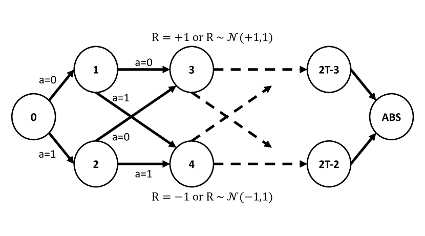
For every environment, we initialize the environment with a fixed horizon length $T$. If the agent reaches a goal before $T$ or if the episode is not over by step $T$, it will transition to an environment-dependent absorbing state where it will stay until time $T$. For a high level description of the environment features, see Table 1.

Figure 6: Graph Environment

Figure 7: Graph-MC Environment

Figure 8: MC Environment, pixel-version. The non-pixel version involves representing the state of the car as the position and velocity.

Figure 9: Enduro Environment

Figure 10: Graph-POMDP Environment. Model-Fail [51] is a special case of this environment where T=2. We also extend the environment to arbitrary horizon which makes it a semi-mdp.

Figure 11: Gridworld environment. Blank spaces indicate areas of a small negative reward, S indicates the starting states, F indicates a field of slightly less negative reward, H indicates a hole of severe penalty, G indicates the goal of positive reward.

F.1 Environment Descriptions

F.1.1 Graph

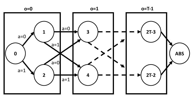
Figure 11 shows a visualization of the Toy-Graph environment. The graph is initialized with horizon $T$ and with absorbing state $x_{abs}=2T$. In each episode, the agent starts at a single starting state $x_{0}=0$ and has two actions, $a=0$ and $a=1$. At each time step $t<T$, the agent can enter state $x_{t+1}=2t+1$ by taking action $a=0$, or $x_{t+1}=2t+2$ by taking action $a=1$. If the environment is stochastic, we simulate noisy transitions by allowing the agent to slip into $x_{t+1}=2t+2$ instead of $x_{t+1}=2t+1$ and vice-versa with probability $.25$. At the final time $t=T$, the agent always enters the terminal state $x_{abs}$. The reward is $+1$ if the agent transitions to an odd state, otherwise is $-1$. If the environment provides sparse rewards, then $r=+1$ if $x_{T-1}$ is odd, $r=-1$ if $x_{T-1}$ is even, otherwise $r=0$. Similarly to deterministic rewards, if the environment’s rewards are stochastic, then the reward is $r\sim N(1,1)$ if the agent transitions to an odd state, otherwise $r\sim N(-1,1)$. If the rewards are sparse and stochastic then $r\sim N(1,1)$ if $x_{T-1}$ is odd, otherwise $r\sim N(-1,1)$ and $r=0$ otherwise.

F.1.2 Graph-POMDP

Figure 11 shows a visualization of the Graph-POMDP environment. The underlying state structure of Graph-POMDP is exactly the Graph environment. However, the states are grouped together based on a choice of Graph-POMDP horizon length, $H$. This parameter groups states into $H$ observable states. The agent only is able to observe among these states, and not the underlying MDP structure. Model-Fail [51] is a special case of this environment when $H=T=2$.

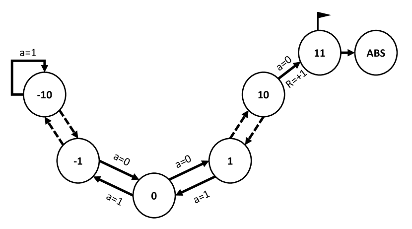
F.1.3 Graph Mountain Car (Graph-MC)

Figure 11 shows a visualization of the Toy-MC environment. This environment is a 1-D graph-based simplification of Mountain Car. The agent starts at $x_{0}=0$, the center of the valley and can go left or right. There are $21$ total states, $10$ to the left of the starting position and $11$ to the right of the starting position, and a terminal absorbing state $x_{abs}=22$. The agent receives a reward of $r=-1$ at every timestep. The reward becomes zero if the agent reaches the goal, which is state $x=+11$. If the agent reaches $x=-10$ and continues left then the agent remains in $x=-10$. If the agent does not reach state $x=+11$ by step $T$ then the episode terminates and the agent transitions to the absorbing state.

F.1.4 Mountain Car (MC)

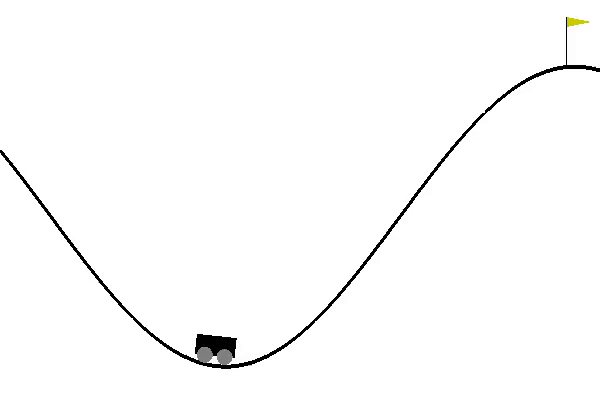
We use the OpenAI version of Mountain Car with a few simplifying modifications [5, 48]. The car starts in a valley and has to go back and forth to gain enough momentum to scale the mountain and reach the end goal. The state space is given by the position and velocity of the car. At each time step, the car has the following options: accelerate backwards, forwards or do nothing. The reward is $r=-1$ for every time step until the car reaches the goal. While the original trajectory length is capped at $200$, we decrease the effective length by applying every action $a_{t}$ five times before observing $x_{t+1}$. Furthermore, we modify the random initial position from being uniformly between $[-.6,-.4]$ to being one of $\{-.6,-.5,-.4\}$, with no velocity. The environment is initialized with a horizon $T$ and absorbing state $x_{abs}=[.5,0],$ position at $.5$ and no velocity.

F.1.5 Pixel-based Mountain Car (Pix-MC)

This environment is identical to Mountain Car except the state space has been modified from position and velocity to a pixel based representation of a ball, representing a car, rolling on a hill, see Figure 11. Each frame $f_{t}$ is a $80\times 120$ image of the ball on the mountain. One cannot deduce velocity from a single frame, so we represent the state as $x_{t}=\{f_{t-1},f_{t}\}$ where $f_{-1}=f_{0},$ the initial state. Everything else is identical between the pixel-based version and the position-velocity version described earlier.

F.1.6 Enduro

We use OpenAI’s implementation of Enduro-v0, an Atari 2600 racing game. We downsample the image to a grayscale of size (84,84). We apply every action one time and we represent the state as $x_{t}=\{f_{t-3},f_{t-2},f_{t-1},f_{t}\}$ where $f_{i}=f_{0},$ the initial state, for $i<0$. See Figure 11 for a visualization.

F.1.7 Gridworld (GW)

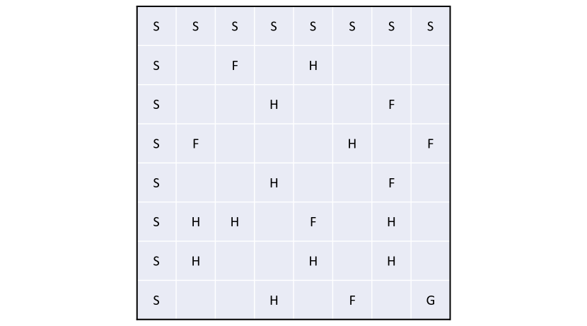
Figure 11 shows a visualization of the Gridworld environment. The agent starts at a state in the first row or column (denoted S in the figure), and proceeds through the grid by taking actions, given by the four cardinal directions, for $T=25$ timesteps. An agent remains in the same state if it chooses an action which would take it out of the environment. If the agent reaches the goal state $G$, in the bottom right corner of the environment, it transitions to a terminal state $x=64$ for the remainder of the trajectory and receives a reward of $+1$. In the grid, there is a field (denoted F) which gives the agent a reward of $-.005$ and holes (denoted H) which give $-.5$. The remaining states give a reward of $-.01$.

F.1.8 Pixel-Gridworld (Pixel-GW)

This environment is identical to Gridworld except the state space has been modified from position to a pixel based representation of the position: 1 for the agent’s location, 0 otherwise. We use the same policies as in the Gridworld case.

Table 17: Environment parameters - Full description

Environment	Graph	Graph-MC	MC	Pix-MC	Enduro	Graph-POMDP	GW	Pix-GW
Is MDP?	yes	yes	yes	yes	yes	no	yes	yes
State desc.	position	position	[pos, vel]	pixels	pixels	position	position	pixels
$T$	4 or 16	250	250	250	1000	2 or 8	25	25
Stoch Env?	variable	no	no	no	no	no	no	variable
Stoch Rew?	variable	no	no	no	no	no	no	no
Sparse Rew?	variable	terminal	terminal	terminal	dense	terminal	dense	dense
$\hat{Q}$ Func. Class	tabular	tabular	linear/NN	NN	NN	tabular	tabular	NN
Initial state	0	0	variable	variable	gray img	0	variable	variable
Absorb. state	2T	22	[.5,0]	img([.5,0])	zero img	2T	64	zero img
Frame height	1	1	2	2	4	1	1	1
Frame skip	1	1	5	5	1	1	1	1

Appendix G Experimental Setup

G.1 Description of the policies

Graph, Graph-POMDP and Graph-MC use static policies with some probability of going left and another probability of going right, ex: $\pi(a=0)=p,\pi(a=1)=1-p$, independent of state. We vary $p$ in our experiments.

GW, Pix-GW, MC, Pixel-MC, and Enduro all use an $\epsilon-$Greedy policy. In other words, we train a policy $Q^{\ast}$ (using value iteration or DDQN) and then vary the deviation away from the policy. Hence $\epsilon-Greedy(Q^{\ast})$ implies we follow a mixed policy $\pi=\operatorname*{arg\,max}_{a}Q^{\ast}(x,a)$ with probability $1-\epsilon$ and uniform with probability $\epsilon$. We vary $\epsilon$ in our experiments.

G.2 Enumeration of Experiments

G.2.1 Graph

See Table G.2.1 for a description of the parameters of the experiment we ran in the Graph Environment. The experiments are the Cartesian product of the table.

Table 18: Graph parameters

	Parameters
$\gamma$	.98
N	$2^{3:11}$
T	$\{4,16\}$
$\pi_{b}(a=0)$	$\{.2,.6\}$
$\pi_{e}(a=0)$	$.8$
Stochastic Env	{True, False}
Stochastic Rew	{True, False}
Sparse Rew	{True, False}
Seed	{10 random}
ModelType	Tabular
Regress $\pi_{b}$	False

G.2.2 Graph-POMDP

See Table G.2.2 for a description of the parameters of the experiment we ran in the Graph-POMDP Environment. The experiments are the Cartesian product of the table.

Table 19: Graph-POMDP parameters

	Parameters
$\gamma$	.98
N	$2^{8:11}$
(T,H)	$\{(2,2),(16,6)\}$
$\pi_{b}(a=0)$	$\{.2,.6\}$
$\pi_{e}(a=0)$	$.8$
Stochastic Env	{True, False}
Stochastic Rew	{True, False}
Sparse Rew	{True, False}
Seed	{10 random}
ModelType	Tabular
Regress $\pi_{b}$	False

G.2.3 Gridworld

See Table G.2.3 for a description of the parameters of the experiment we ran in the Gridworld Environment. The experiments are the Cartesian product of the table.

Table 20: Gridworld parameters

	Parameters
$\gamma$	.98
N	$2^{6:11}$
T	$25$
$\epsilon-\text{Greedy},\pi_{b}$	$\{.2,.4,.6,.8,1.\}$
$\epsilon-\text{Greedy},\pi_{e}$	$.1$
Stochastic Env	False
Stochastic Rew	False
Sparse Rew	False
Seed	{10 random}
ModelType	Tabular
Regress $\pi_{b}$	True

G.2.4 Pixel-Gridworld (Pix-GW)

See Table G.2.4 for a description of the parameters of the experiment we ran in the Pix-GW Environment. The experiments are the Cartesian product of the table.

Table 21: Pix-GW parameters

	Parameters
$\gamma$	.96
N	$2^{6:9}$
T	$25$
$\epsilon-\text{Greedy},\pi_{b}$	$\{.2,.4,.6,.8,1.\}$
$\epsilon-\text{Greedy},\pi_{e}$	$.1$
Stochastic Env	{True, False}
Stochastic Rew	False
Sparse Rew	False
Seed	{10 random}
ModelType	NN
Regress $\pi_{b}$	{True, False}

G.2.5 Graph-MC

See Table G.2.5 for a description of the parameters of the experiment we ran in the TMC Environment. The experiments are the Cartesian product of the table.

Table 22: Graph-MC parameters

	Parameters
$\gamma$	.99
N	$2^{7:11}$
T	$250$
$(\pi_{b}(a=0),\pi_{e}(a=0))$	$\{(.45,.45),(.6,.6),(.45.6)$
	$(.6,.45),(.8,.2),(.2,.8)\}$
Stochastic Env	False
Stochastic Rew	False
Sparse Rew	False
Seed	{10 random}
ModelType	Tabular
Regress $\pi_{b}$	False

G.2.6 Mountain Car (MC)

See Table G.2.6 for a description of the parameters of the experiment we ran in the MC Environment. The experiments are the Cartesian product of the table.

Table 23: MC parameters

	Parameters
$\gamma$	.99
N	$2^{7:10}$
T	$250$
$\epsilon-\text{Greedy},(\pi_{b},\pi_{e})$	$\{(.1,0),(1,0)$
	$(1,.1),(.1,1)\}$
Stochastic Env	False
Stochastic Rew	False
Sparse Rew	False
Seed	{10 random}
ModelType	{Tabular, NN}
Regress $\pi_{b}$	False

G.2.7 Pixel-Mountain Car (Pix-MC)

See Table G.2.7 for a description of the parameters of the experiment we ran in the Pix-MC Environment. The experiments are the Cartesian product of the table.

Table 24: Pix-MC parameters

	Parameters
$\gamma$	.97
N	$512$
T	$500$
$\epsilon-\text{Greedy},(\pi_{b},\pi_{e})$	$\{(.25,0),(.1,0)$
	$(.25,.1)\}$
Stochastic Env	False
Stochastic Rew	False
Sparse Rew	False
Seed	{10 random}
ModelType	{Tabular, NN}
Regress $\pi_{b}$	False

G.2.8 Enduro

See Table G.2.8 for a description of the parameters of the experiment we ran in the Enduro Environment. The experiments are the Cartesian product of the table.

Table 25: Enduro parameters

	Parameters
$\gamma$	.9999
N	$512$
T	$500$
$\epsilon-\text{Greedy},(\pi_{b},\pi_{e})$	$\{(.25,0),(.1,0)$
	$(.25,.1)\}$
Stochastic Env	False
Stochastic Rew	False
Sparse Rew	False
Seed	{10 random}
ModelType	{Tabular, NN}
Regress $\pi_{b}$	False

G.3 Representation and Function Class

For the simpler environments, we use a tabular representation for all the methods. AM amounts to solving for the transition dynamics, rewards, terminal state, etc. through maximum likelihood. FQE, Retrace($\lambda$), $Q^{\pi}(\lambda)$, and Tree-Backup are all implemented through dynamics programming with Q tables. MRDR and Q-Reg used the Sherman Morrison [47] method to solve the weighted-least square problem, using a basis which spans a table.

In the cases where we needed function approximation, we did not directly fit the dynamics for AM; instead, we fit on the difference in states $P(x^{\prime}-x|x,a)$, which is common practice.

For the MC environment, we ran experiments with both a linear and NN function class. In both cases, the representation of the state was not changed and remained [position, velocity]. The NN architecture was dense with [16,8,4,2] as the layers. The layers had relu activations (except the last, with a linear activation) and were all initialized with truncated normal centered at 0 with a standard deviation of 0.1.

For the pixel-based environments (MC, Enduro), we use a convolutional NN. The architechure is a layer of size 8 with filter (7,7) and stride 3, followed by maxpooling and a layer of size 16 with filter (3,3) and stride 1, followed by max pooling, flattening and a dense layer of size 256. The final layer is a dense layer with the size of the action space, with a linear activation. The layers had elu activations and were all initialized with truncated normal centered at 0 with a standard deviation of 0.1. The layers also have kernel L2 regularizers with weight 1e-6.

When using NNs for the IH method, we used the radial-basis function and a shallow dense network for the kernel and density estimate respectively.

G.4 Datasets

Datasets are not included as part of COBS since our benchmark is completely simulation based. To recreate any dataset, select the appropriate choice of environment parameters from the experiments enumerated in Section G.2.

G.5 Choice of hyperparameters

Many methods require selection of convergence criteria, regularization parameters, batch sizes, and a whole host of other hyperparameters. Often there is a trade-off between computational cost and the accuracy of the method. Hyperparameter search is not feasible in OPE since there is no proper validation (like game score in learning). See Table G.5 for a list of hyperparameters that were chosen for the experiments.

Figure 12: Hyperparameters for each model by Environment

Method	Parameter	Graph	TMC	MC	Pix-MC	Enduro	Graph-POMDP	GW	Pix-GW
AM	Max Traj Len	T	T	50	50	-	T	T	T
	NN Fit Epochs	-	-	100	100	-	-	-	100
	NN Batchsize	-	-	32	32	-	-	-	25
	NN Train size	-	-	.8	.8	-	-	-	.8
	NN Val size	-	-	.2	.2	-	-	-	.2
	NN Early Stop delta	-	-	1e-4	1e-4	-	-	-	1e-4
Q-Reg	Omega regul.	1	1	-	-	-	1	1	-
	NN Fit Epochs	-	-	80	80	80	-	-	80
	NN Batchsize	-	-	32	32	32	-	-	32
	NN Train size	-	-	.8	.8	.8	-	-	.8
	NN Val size	-	-	.2	.2	.2	-	-	.2
	NN Early Stop delta	-	-	1e-4	1e-4	1e-4	-	-	1e-4
FQE	Convergence $\epsilon$	1e-5	1e-5	1e-4	1e-4	1e-4	1e-5	4e-4	1e-4
	Max Iter	-	-	160	160	600	-	50	80
	NN Batchsize	-	-	32	32	32	-	-	32
	Optimizer Clipnorm	-	-	1.	1.	1.	-	-	1.
IH	Quad. prog. regular.	1e-3	1e-3	-	-	-	1e-3	1e-3	-
	NN Fit Epochs	-	-	10001	10001	10001	-	-	1001
	NN Batchsize	-	-	1024	128	128	-	-	128
MRDR	Omega regul.	1	1	-	-	-	1	1	-
	NN Fit Epochs	-	-	80	80	80	-	-	80
	NN Batchsize	-	-	1024	1024	1024	-	-	32
	NN Train size	-	-	.8	.8	.8	-	-	.8
	NN Val size	-	-	.2	.2	.2	-	-	.2
	NN Early Stop delta	-	-	1e-4	1e-4	1e-4	-	-	1e-4
$R(\lambda)$	$\lambda$	.9	.9	.9	-	-	.9	.9	.9
	Convergence $\epsilon$	1e-3	2e-3	1e-3	-	-	1e-3	2e-3	1e-3
	Max Iter	500	500	-	-	-	500	50	-
	NN Fit Epochs	-	-	80	-	-	-	-	80
	NN Batchsize	-	-	4	-	-	-	-	4
	NN Train Size	-	-	.03	-	-	-	-	.03
	NN ClipNorm	-	-	1.	-	-	-	-	1.
$Q^{\pi}(\lambda)$	$\lambda$	.9	.9	.9	-	-	.9	.9	.9
	Convergence $\epsilon$	1e-3	2e-3	1e-3	-	-	1e-3	2e-3	1e-3
	Max Iter	500	500	-	-	-	500	50	-
	NN Fit Epochs	-	-	80	-	-	-	-	80
	NN Batchsize	-	-	4	-	-	-	-	4
	NN Train Size	-	-	.03	-	-	-	-	.03
	NN ClipNorm	-	-	1.	-	-	-	-	1.
Tree	$\lambda$	.9	.9	.9	-	-	.9	.9	.9
	Convergence $\epsilon$	1e-3	2e-3	1e-3	-	-	1e-3	2e-3	1e-3
	Max Iter	500	500	-	-	-	500	50	-
	NN Fit Epochs	-	-	80	-	-	-	-	80
	NN Batchsize	-	-	4	-	-	-	-	4
	NN Train Size	-	-	.03	-	-	-	-	.03
	NN ClipNorm	-	-	1.	-	-	-	-	1.

Appendix H Additional Supporting Figures

Figure 13: Enduro DM vs IPS. $\pi_{b}$ is a policy that deviates uniformly from a trained policy $25\%$ of the time, $\pi_{e}$ is a policy trained with DDQN. IH has relatively low error mainly due to tracking the simple average, since the kernel function did not learn useful density ratio. The computational time required to calculate the multi-step rollouts of AM, Retrace($\lambda$), $Q^{\pi}(\lambda)$, Tree-Backup($\lambda$) exceeded our compute budget and were thus excluded.

Figure 14: MC comparison. $N=256$. $\pi_{b}$ is a uniform random policy, $\pi_{e}$ is a policy trained with DDQN

Figure 15: Enduro DM vs HM. $\pi_{b}$ is a policy that deviates uniformly from a trained policy $25\%$ of the time, $\pi_{e}$ is a policy trained with DDQN.

Figure 16: Comparison of Direct methods’ performance across horizon and number of trajectories in the Toy-Graph environment. Small policy mismatch under a deterministic environment.

Figure 17: (Graph domain) Comparing DMs across horizon length and number of trajectories. Large policy mismatch and a stochastic environment setting.

Figure 18: Comparing DM to DR in a stochastic environment with large policy mismatch. (Graph)

Figure 19: Comparison between FQE, IH and WIS in a low data regime. For low policy mismatch, IPS is competitive to DM in low data, but as the policy mismatch grows, the top DM outperform. Experiments ran in the Gridworld Environment.

Figure 20: Comparison between IPS methods and IH with dense vs sparse rewards. Per-Decision IPS methods see substantial improvement when the rewards are dense. Experiments ran in the Toy-Graph environment with $\pi(a=0)=.6,\pi_{e}(a=0)=.8$

Figure 21: Exact vs Estimated $\pi_{b}$. Exact $\pi_{b}=.2-$Greedy(optimal), $\pi_{e}=.1-$Greedy(optimal). Min error per class. (Pixel Gridworld, deterministic)

Figure 22: Exact vs Estimated $\pi_{b}$. Exact $\pi_{b}=$uniform, $\pi_{e}=.1-$Greedy(optimal). Min error per class. (Pixel Gridworld, deterministic)

Figure 23: Hybrid Method comparison. $\pi_{b}(a=0)=.2,\pi_{e}(a=0)=.8$. Min error per class. (Graph-MC)

Figure 24: Hybrid Method comparison. $\pi_{b}(a=0)=.8,\pi_{e}(a=0)=.2$. Min error per class. (Graph-MC)

Figure 25: Hybrid Method comparison. $\pi_{b}(a=0)=.6,\pi_{e}(a=0)=.6$. Min error per class. (Graph-MC)

Figure 26: Hybrid Method comparison. Exact $\pi_{b}=.2-$Greedy(optimal), $\pi_{e}=.1-$Greedy(optimal). Min error per class. (Pixel Gridworld)

Figure 27: Hybrid Method comparison. $\pi_{b}=.8-$Greedy(optimal), $\pi_{e}=.1-$Greedy(optimal). Min error per class. (Pixel Gridworld)

Figure 28: Class comparison with unknown $\pi_{b}$. At first, HM underperform DM because $\pi_{b}$ is more difficult to calculate leading to imprecise importance sampling estimates. Exact $\pi_{b}=.2-$Greedy(optimal), $\pi_{e}=.1-$Greedy(optimal). Min error per class. (Pixel Gridworld, stochastic env with .2 slippage)

Figure 29: Class comparison with unknown $\pi_{b}$. At first, HM underperform DM because $\pi_{b}$ is more difficult to calculate leading to imprecise importance sampling estimates. Exact $\pi_{b}=.6-$Greedy(optimal), $\pi_{e}=.1-$Greedy(optimal). Min error per class. (Pixel Gridworld, stochastic env with .2 slippage)

Figure 30: Class comparison with unknown $\pi_{b}$. At first, HM underperform DM because $\pi_{b}$ is more difficult to calculate leading to imprecise importance sampling estimates. Exact $\pi_{b}=$uniform, $\pi_{e}=.1-$Greedy(optimal). Min error per class. (Pixel Gridworld, stochastic env with .2 slippage)

Figure 31: AM Direct vs Hybrid comparison for AM. (Gridworld)

Figure 32: FQE Direct vs Hybrid comparison. (Gridworld)

Figure 33: MRDR Direct vs Hybrid comparison. (Gridworld)

Figure 34: Q-Reg Direct vs Hybrid comparison. (Gridworld)

Figure 35: $Q^{\pi}(\lambda)$ Direct vs Hybrid comparison. (Gridworld)

Figure 36: Retrace$(\lambda)$ Direct vs Hybrid comparison. (Gridworld)

Figure 37: Tree-Backup Direct vs Hybrid comparison. (Gridworld)

Figure 38: DR comparison with $\pi_{b}=.2-$Greedy(optimal), $\pi_{e}=1.-$Greedy(optimal). (Pixel Gridworld)

Figure 39: WDR comparison with $\pi_{b}=.2-$Greedy(optimal), $\pi_{e}=1.-$Greedy(optimal). (Pixel Gridworld)

Figure 40: MAGIC comparison with $\pi_{b}=.2-$Greedy(optimal), $\pi_{e}=1.-$Greedy(optimal). (Pixel Gridworld)

Figure 41: DR comparison with $\pi_{b}=.8-$Greedy(optimal), $\pi_{e}=1.-$Greedy(optimal). (Pixel Gridworld)

Figure 42: WDR comparison with $\pi_{b}=.8-$Greedy(optimal), $\pi_{e}=1.-$Greedy(optimal). (Pixel Gridworld)

Figure 43: MAGIC comparison with $\pi_{b}=.8-$Greedy(optimal), $\pi_{e}=1.-$Greedy(optimal). (Pixel Gridworld)

Appendix I Complete Results

For tables of the complete results of the experiments, please see the COBS github page: https://github.com/clvoloshin/COBS.

References

- [1] Heejung Bang and James M. Robins. Doubly robust estimation in missing data and causal inference models. Biometrics, 61(4):962–973, 2005.
- [2] Marc G Bellemare, Yavar Naddaf, Joel Veness, and Michael Bowling. The arcade learning environment: An evaluation platform for general agents. Journal of Artificial Intelligence Research, 47:253–279, 2013.
- [3] Léon Bottou, Jonas Peters, Joaquin Qui nonero Candela, Denis X. Charles, D. Max Chickering, Elon Portugaly, Dipankar Ray, Patrice Simard, and Ed Snelson. Counterfactual reasoning and learning systems: The example of computational advertising. Journal of Machine Learning Research (JMLR), 14:3207–3260, 2013.
- [4] Greg Brockman, Vicki Cheung, Ludwig Pettersson, Jonas Schneider, John Schulman, Jie Tang, and Wojciech Zaremba. Openai gym. arXiv preprint arXiv:1606.01540, 2016.
- [5] Greg Brockman, Vicki Cheung, Ludwig Pettersson, Jonas Schneider, John Schulman, Jie Tang, and Wojciech Zaremba. Openai gym, 2016.
- [6] Rich Caruana, Nikos Karampatziakis, and Ainur Yessenalina. An empirical evaluation of supervised learning in high dimensions. In Proceedings of the 25th international conference on Machine learning, pages 96–103, 2008.
- [7] Rich Caruana and Alexandru Niculescu-Mizil. An empirical comparison of supervised learning algorithms. In Proceedings of the 23rd international conference on Machine learning, pages 161–168, 2006.
- [8] Olivier Chapelle and Lihong Li. An empirical evaluation of thompson sampling. In Advances in neural information processing systems, pages 2249–2257, 2011.
- [9] Jinglin Chen and Nan Jiang. Information-theoretic considerations in batch reinforcement learning. In International Conference on Machine Learning (ICML), 2019.
- [10] Bo Dai, Ofir Nachum, Yinlam Chow, Lihong Li, Csaba Szepesvári, and Dale Schuurmans. Coindice: Off-policy confidence interval estimation. arXiv preprint arXiv:2010.11652, 2020.
- [11] Christoph Dann, Gerhard Neumann, Jan Peters, et al. Policy evaluation with temporal differences: A survey and comparison. Journal of Machine Learning Research, 15:809–883, 2014.
- [12] Thomas Degris, Martha White, and Richard S Sutton. Off-policy actor-critic. 2012.
- [13] Jia Deng, Wei Dong, Richard Socher, Li-Jia Li, Kai Li, and Li Fei-Fei. Imagenet: A large-scale hierarchical image database. In IEEE Conference on Computer Vision and Pattern Recognition (CVPR), pages 248–255, 2009.
- [14] Yan Duan, Xi Chen, Rein Houthooft, John Schulman, and Pieter Abbeel. Benchmarking deep reinforcement learning for continuous control. In International Conference on Machine Learning (ICML), 2016.
- [15] Miroslav Dudík, John Langford, and Lihong Li. Doubly robust policy evaluation and learning. In International Conference on Machine Learning (ICML), 2011.
- [16] Mehrdad Farajtabar, Yinlam Chow, and Mohammad Ghavamzadeh. More robust doubly robust off-policy evaluation. In International Conference on Machine Learning (ICML), 2018.
- [17] Justin Fu, Aviral Kumar, Ofir Nachum, George Tucker, and Sergey Levine. D4rl: Datasets for deep data-driven reinforcement learning, 2020.
- [18] Justin Fu, Mohammad Norouzi, Ofir Nachum, George Tucker, ziyu wang, Alexander Novikov, Mengjiao Yang, Michael R Zhang, Yutian Chen, Aviral Kumar, Cosmin Paduraru, Sergey Levine, and Thomas Paine. Benchmarks for deep off-policy evaluation. In International Conference on Learning Representations, 2021.
- [19] Jason Gauci, Edoardo Conti, Yitao Liang, Kittipat Virochsiri, Zhengxing Chen, Yuchen He, Zachary Kaden, Vivek Narayanan, and Xiaohui Ye. Horizon: Facebook’s open source applied reinforcement learning platform. arXiv preprint arXiv:1811.00260, 2018.
- [20] John Michael Hammersley and David Christopher Handscomb. Monte carlo methods. 1964.
- [21] Anna Harutyunyan, Marc G. Bellemare, Tom Stepleton, and Rémi Munos. Q(lambda) with off-policy corrections. In Conference on Algorithmic Learning Theory (ALT), 2016.
- [22] Hado van Hasselt, Arthur Guez, and David Silver. Deep reinforcement learning with double q-learning. In Proceedings of the Thirtieth AAAI Conference on Artificial Intelligence, AAAI’16, page 2094–2100. AAAI Press, 2016.
- [23] Peter Henderson, Riashat Islam, Philip Bachman, Joelle Pineau, Doina Precup, and David Meger. Deep reinforcement learning that matters. In Thirty-Second AAAI Conference on Artificial Intelligence, 2018.
- [24] Daniel G Horvitz and Donovan J Thompson. A generalization of sampling without replacement from a finite universe. Journal of the American statistical Association, 47(260):663–685, 1952.
- [25] Nan Jiang and Jiawei Huang. Minimax value interval for off-policy evaluation and policy optimization. In H. Larochelle, M. Ranzato, R. Hadsell, M. F. Balcan, and H. Lin, editors, Advances in Neural Information Processing Systems, volume 33, pages 2747–2758. Curran Associates, Inc., 2020.
- [26] Nan Jiang and Lihong Li. Doubly robust off-policy value evaluation for reinforcement learning. In International Conference on Machine Learning (ICML), 2016.
- [27] Nathan Kallus and Masatoshi Uehara. Double reinforcement learning for efficient off-policy evaluation in markov decision processes. arXiv preprint arXiv:1908.08526, 2019.
- [28] Nathan Kallus and Masatoshi Uehara. Efficiently breaking the curse of horizon: Double reinforcement learning in infinite-horizon processes. arXiv preprint arXiv:1909.05850, 2019.
- [29] Joseph DY Kang, Joseph L Schafer, et al. Demystifying double robustness: A comparison of alternative strategies for estimating a population mean from incomplete data. Statistical science, 22(4):523–539, 2007.
- [30] Hoang M Le, Cameron Voloshin, and Yisong Yue. Batch policy learning under constraints. In International Conference on Machine Learning (ICML), 2019.
- [31] Lihong Li, Wei Chu, John Langford, and Xuanhui Wang. Unbiased offline evaluation of contextual-bandit-based news article recommendation algorithms. In ACM Conference on Web Search and Data Mining (WSDM), 2011.
- [32] Lihong Li, Rémi Munos, and Csaba Szepesvári. Toward minimax off-policy value estimation. In Artificial Intelligence and Statistics, pages 608–616, 2015.
- [33] Qiang Liu, Lihong Li, Ziyang Tang, and Dengyong Zhou. Breaking the curse of horizon: Infinite-horizon off-policy estimation. In Neural Information Processing Systems (NeurIPS), 2018.
- [34] Yao Liu, Adith Swaminathan, Alekh Agarwal, and Emma Brunskill. Off-policy policy gradient with state distribution correction. arXiv preprint arXiv:1904.08473, 2019.
- [35] Francesco Locatello, Stefan Bauer, Mario Lucic, Gunnar Raetsch, Sylvain Gelly, Bernhard Schölkopf, and Olivier Bachem. Challenging common assumptions in the unsupervised learning of disentangled representations. In International Conference on Machine Learning, pages 4114–4124, 2019.
- [36] Jiaqi Ma, Zhe Zhao, Xinyang Yi, Ji Yang, Minmin Chen, Jiaxi Tang, Lichan Hong, and Ed H Chi. Off-policy learning in two-stage recommender systems. In International World Wide Web Conference (WWW), 2020.
- [37] Remi Munos, Tom Stepleton, Anna Harutyunyan, and Marc Bellemare. Safe and efficient off-policy reinforcement learning. In Neural Information Processing Systems (NeurIPS). 2016.
- [38] Rémi Munos and Csaba Szepesvári. Finite-time bounds for fitted value iteration. Journal of Machine Learning Research (JMLR), 9(May):815–857, 2008.
- [39] Susan A Murphy, Mark J van der Laan, James M Robins, and Conduct Problems Prevention Research Group. Marginal mean models for dynamic regimes. Journal of the American Statistical Association, 96(456):1410–1423, 2001.
- [40] Ofir Nachum, Yinlam Chow, Bo Dai, and Lihong Li. Dualdice: Behavior-agnostic estimation of discounted stationary distribution corrections. In Advances in Neural Information Processing Systems, pages 2315–2325, 2019.
- [41] Xinkun Nie, Emma Brunskill, and Stefan Wager. Learning when-to-treat policies. arXiv preprint arXiv:1905.09751, 2019.
- [42] Michael Oberst and David Sontag. Counterfactual off-policy evaluation with gumbel-max structural causal models. In International Conference on Machine Learning, pages 4881–4890, 2019.
- [43] Cosmin Paduraru. Off-policy evaluation in Markov decision processes. PhD thesis, McGill University Libraries, 2013.
- [44] Michael JD Powell and J Swann. Weighted uniform sampling—a monte carlo technique for reducing variance. IMA Journal of Applied Mathematics, 2(3):228–236, 1966.
- [45] Doina Precup, Richard S. Sutton, and Satinder P. Singh. Eligibility traces for off-policy policy evaluation. In International Conference on Machine Learning (ICML), 2000.
- [46] Yuta Saito, Shunsuke Aihara, Megumi Matsutani, and Yusuke Narita. A large-scale open dataset for bandit algorithms. arXiv preprint arXiv:2008.07146, 2020.
- [47] Jack Sherman and Winifred J. Morrison. Adjustment of an inverse matrix corresponding to a change in one element of a given matrix. Ann. Math. Statist., 21(1):124–127, 03 1950.
- [48] Richard S Sutton and Andrew G Barto. Reinforcement learning: An introduction. MIT press, 2018.
- [49] Adith Swaminathan, Akshay Krishnamurthy, Alekh Agarwal, Miro Dudik, John Langford, Damien Jose, and Imed Zitouni. Off-policy evaluation for slate recommendation. In Neural Information Processing Systems (NeurIPS). 2017.
- [50] Guy Tennenholtz, Shie Mannor, and Uri Shalit. Off-policy evaluation in partially observable environments. arXiv preprint arXiv:1909.03739, 2019.
- [51] Philip Thomas and Emma Brunskill. Data-efficient off-policy policy evaluation for reinforcement learning. In International Conference on Machine Learning (ICML), 2016.
- [52] Philip S Thomas, Georgios Theocharous, Mohammad Ghavamzadeh, Ishan Durugkar, and Emma Brunskill. Predictive off-policy policy evaluation for nonstationary decision problems, with applications to digital marketing. In AAAI Conference on Innovative Applications (IAA), 2017.
- [53] Emanuel Todorov, Tom Erez, and Yuval Tassa. Mujoco: A physics engine for model-based control. In 2012 IEEE/RSJ International Conference on Intelligent Robots and Systems, pages 5026–5033. IEEE, 2012.
- [54] Masatoshi Uehara, Jiawei Huang, and Nan Jiang. Minimax weight and q-function learning for off-policy evaluation. In International Conference on Machine Learning, pages 9659–9668. PMLR, 2020.
- [55] Cameron Voloshin, Nan Jiang, and Yisong Yue. Minimax model learning. In International Conference on Artificial Intelligence and Statistics, pages 1612–1620. PMLR, 2021.
- [56] Yu-Xiang Wang, Alekh Agarwal, and Miroslav Dudík. Optimal and adaptive off-policy evaluation in contextual bandits. In International Conference on Machine Learning (ICML), 2017.
- [57] MA Wiering. Multi-agent reinforcement learning for traffic light control. In International Conference on Machine Learning (ICML), 2000.
- [58] Tengyang Xie, Yifei Ma, and Yu-Xiang Wang. Towards optimal off-policy evaluation for reinforcement learning with marginalized importance sampling. In Advances in Neural Information Processing Systems, pages 9665–9675, 2019.
- [59] Mengjiao Yang, Ofir Nachum, Bo Dai, Lihong Li, and Dale Schuurmans. Off-policy evaluation via the regularized lagrangian. Advances in Neural Information Processing Systems, 33, 2020.
- [60] Michael R Zhang, Tom Le Paine, Ofir Nachum, Cosmin Paduraru, George Tucker, Ziyu Wang, and Mohammad Norouzi. Autoregressive dynamics models for offline policy evaluation and optimization. arXiv preprint arXiv:2104.13877, 2021.
- [61] Shangtong Zhang, Bo Liu, and Shimon Whiteson. Gradientdice: Rethinking generalized offline estimation of stationary values. arXiv preprint arXiv:2001.11113, 2020.
- [62] Stephan Zheng, Alexander Trott, Sunil Srinivasa, Nikhil Naik, Melvin Gruesbeck, David C Parkes, and Richard Socher. The ai economist: Improving equality and productivity with ai-driven tax policies. arXiv preprint arXiv:2004.13332, 2020.