GFiRe Gauge Field integrator for Reheating

Abstract

We present a new numerical algorithm and code, ${\sf GFiRe}$, for solving the non-linear evolution of Abelian gauge fields coupled to complex scalar fields in homogeneous and isotropic spacetimes. We adopt a hybrid approach to solving the system: the spatial derivatives are discretized using standard Lattice Gauge Field Theory techniques, whereas the time evolution of the fields and scale factor is implemented with explicit, composite, symplectic integrators. An important property of our compound algorithm is that the discretized Gauss constraint is respected exactly, regardless of the order of the symplectic integrator. This remains true even when the background expansion is computed “self-consistently”; that is, when the expansion history is computed using spatial averaged components of the energy momentum tensor in the simulation volume. Hence, our code can also be used in cases where the fields dominate the energy density of the universe, for example, during reheating after inflation.

We test the algorithm in scenarios of reheating where the inflaton is a complex scalar field with a potential $\propto(2|\varphi|^{2}-v^{2})^{2}$ and is coupled to an Abelian gauge field. Tracing the evolution of the system through complex dynamics (including resonant excitation of fields, backreaction, formation of solitons, and changes in the equation of state) in a self-consistently expanding universe, we find the energy conservation violation ($<10^{-4}$) to be very stable and the Gauss constraint violation ($<10^{-6}$) to be dominated by differencing noise.

1 Introduction

Reheating after inflation is an integral part of the inflationary scenario (see, for example, [1, 2, 3, 4, 5, 6, 7, 8, 9, 10]). Non-nonlinear dynamics during reheating can lead to novel phenomenon such as: (i) changes in the post-inflationary equation of state (e.g., [11, 12, 13]), (ii) formation of defects (for example, cosmic strings [14, 15]) and solitons (e.g., oscillons, [15, 16, 17], and related structures [18, 19, 20, 21]), (iii) production of non-gaussian gravitational perturbations (e.g., [22, 23, 24]), (iv) stochastic gravitational waves (e.g., [25, 26, 27, 28, 29, 30, 31, 32, 33, 34, 35, 36, 37, 38, 39, 40, 41, 42, 43, 44]), and (v) formation of primordial black holes (e.g., [45, 46, 47, 48, 49, 50, 51, 52, 53, 54]). Many non-thermal and nonlinear phenomena during reheating can potentially change abundances of relics such as dark matter and baryon asymmetry (e.g., [55, 56, 57, 58]).

The details of the nonlinear phenomena are often hard to infer directly from from analytic considerations, making numerical simulations necessary in many cases. The non-trivial scale dependence arising from non-perturbative dynamics can provide insights into the best observational strategies to probe new physics from this era. To have confidence in new phenomena discovered in the simulations, and their observational implications, the numerical algorithms and simulations must satisfy known analytic constraints and the numerical errors must be under control. It is therefore important to develop techniques for studying the nonlinear evolution of fields as accurately as possible. Moreover, many techniques developed for studying nonlinear dynamics of fields in reheating, can be applied to other eras in the early universe including phase transitions (e.g. [59]), moduli dynamics (e.g [60, 61]) and also to the dynamics of axion/axion-like fields (e.g. [62, 63, 19, 64, 65, 66]) and even in the context of resolving the Hubble tension [67].

Gauge fields are present in the Standard Model and its extensions, for example the photon, $W$ and $Z$ bosons. They can have highly nonlinear dynamics during reheating, partly due to their Bosonic nature. Their simulations, however, are challenging – first because of the increase in the number of dynamical degrees of freedom, but more importantly, because of the requirement of preserving certain additional constraints (for example, the Gauss constraint) during the time evolution. In this work, we provide an algorithm and code, ${\sf GFiRe}$ – a Gauge Field Integrator for Reheating which is capable of simulating a system of charged scalar fields and Abelian Gauge fields on a lattice in an homogeneous and isotropic, expanding universe. ${\sf GFiRe}$ preserves the Gauss constraint and energy constraint exceptionally well; this remains true even when the expansion is determined self-consistently by the spatially averaged energy momentum tensor at each time step. Our time evolution is symplectic and explicit in time.

Below, we briefly review some relevant literature on nonlinear dynamics of cosmological fields (mostly in the context of reheating), and put our current work in context of the existing literature – highlighting the new and useful aspects of our present work.

Exploring the nonlinear dynamics of scalar fields during reheating is not new. Soon after the importance of non-adiabatic particle production in the oscillating inflaton background was appreciated (a phenomenon known as preheating [2, 3, 4, 5]), it was realized that the subsequent backreaction can lead to a complex, non-linear evolution of the combined inflaton-daughter fields system. For some of the earliest scalar field simulations in the reheating context, see [68, 69]. Since then, a number of dedicated lattice codes have been developed for scalar field models. Most of them are based on finite-differencing techniques, e.g., LatticeEasy [70], Defrost [71], HLattice [72], PyCool [73], Gabe [74], but there are also pseudo-spectral ones, e.g., PSpectRe [75] and Stella [76]. Usually, the codes solve the evolution of a system of spatially inhomogeneous, (self-)interacting scalar-field(s) in a spatially homogeneous and isotropic spacetime. In many cases, the expansion rate is determined self-consistently from the acceleration equation, with appropriate preservation of the energy constraint (i.e., the Friedmann equation is satisfied).

Beyond scalar fields, lattice simulations of gauge fields have also been carried out. These scenarios can be split into two groups depending on the nature of the scalar coupled to the gauge fields: (i) the scalar is uncharged ($\chi$), and (ii) the scalar is charged ($\varphi$).

For an uncharged scalar + Abelian gauge fields systems, Lagrangians which include couplings of the form $\chi F\tilde{F}$ [85, 86, 87, 88, 89, 90, 91], and $f(\chi)F^{2}$ [92] have been simulated in the context of reheating. For non-Abelian fields, $\mathcal{L}\supset f(\chi)\rm{tr\boldsymbol{F}^{2}}$ [93] has been explored. In [88, 89, 90], gauge invariance at the level of the spatially discretized action is guaranteed by the use of slightly modified Link Variables [94], and the Gauss constraint is preserved during the time evolution. The expansion of the universe is obtained from the spatially averaged energy density. However, their algorithm (which works in the temporal gauge), required that the integration in time is implicit. On the other hand, the authors in [85, 86, 87] use an explicit time evolution scheme. A Lorenz gauge is used, where all gauge degrees of freedom are made dynamical. Gauge invariance at the level of the spatially discretized action, and the preservation of the Lorenz gauge condition by time evolution is not guaranteed, however, the Lorenz gauge condition is carefully checked a-posteriori after solving the equations of motion on the lattice. The expansion of the universe is once again determined self-consistently.

For the case of charged scalar and gauge fields, lattice simulations with Abelian [95, 27, 96, 97, 98] and non-Abelian [99, 100, 101, 102, 103, 104, 105, 106] gauge fields have been carried where the spatially discretized action, and the time evolution respects the Gauss constraint by using standard Link Variables. However, these simulations assume that the scalar and gauge fields are spectators (i.e., energetically subdominant). The energy constraint in an expanding universe is not relevant in these studies since they assume that the Friedmann-Robertson-Walker (FRW) expansion is determined by an unrelated component of the Universe, e.g., a dark matter component or a thermal bath. The evolution of the scale factor is set to a fixed power-law, $a(\tau)\propto\tau^{p}$ (for example, with $p=1$ for radiation domination).

Our present algorithm and code, GFiRe, includes and adds to the desirable features that appear separately in the above mentioned works. In particular, some of its attractive features include:

• Our discretized action respects a residual gauge invariance related to time-independent gauge transformations (we work in a gauge where the time component of the gauge field is set to zero). This is achieved by using Link Variables for the spatial discretization. The Gauss constraint follows naturally from residual symmetries of the spatially discretized action.

• Our time evolution scheme is explicit in time, and also symplectic. This scheme treats the time evolution of the scale factor (whose equations of motion involve spatial averaging of the energy momentum tensor) in the same way it treats the time evolution of the fields.

• We show that our symplectic time evolution scheme (of the scale factor and fields) preserves the Gauss constraint. We show explicitly that the Gauss constraint is respected exactly by non-linear symplectic integrators of arbitrary order. This result allows us to take advantage of the properties of high order symplectic integrators, for example, excellent stability and conservation for relatively large time steps without the need to worry about spurious gauge modes.

We note that when the charged scalar is the inflaton, or more generally, when the fields dominate the energy density of the universe, solving accurately for the FRW expansion and the equation-of-state can be important for the observational consequences of reheating [13, 12, 29, 30]. Such calculations can substantially reduce uncertainties in inflationary observables such as the tensor-to-scalar ratio, $r$, and the spectral index $n_{\rm s}$ [13]. Self-consistent expansion with good energy-constraint preservation can also be important for studies of non-gaussianity [22, 23].

The paper is organized as follows. In Section 2 we set the scene for the symplectic integrators. After reviewing the generic equations of motion of the model, we rewrite the system in a Hamiltonian form and discretize it on a spatial lattice. In Section 3 we introduce the symplectic integrator algorithm and apply it to the Hamiltonian lattice system. We present the results from two test studies with our new algorithm in Section 4. Section 5 is devoted to concluding remarks and a discussion. Throughout the paper we use natural units in which $c=\hbar=1$ and the reduced Planck mass is $m_{\mbox{\tiny{Pl}}}=1/\sqrt{8\pi G}$. For the metric, we use the $+---$ signature.

2 Scalar Electrodynamics

We consider classical scalar Electrodynamics, also known as the Abelian-Higgs or the Ginzburg-Landau model, with a general Higgs potential. The action for this theory is

$$S=\int d^{4}x\sqrt{-g}\mathcal{L}=\int d^{4}x\sqrt{-g}\left[-\frac{m_{\mbox{\tiny{Pl}}}^{2}}{2}R+|\mathcal{D}\varphi|^{2}-\frac{1}{4e^{2}}F_{\mu\nu}F^{\mu\nu}-\mathcal{V}(|\varphi|)\right]\,,$$ (2.1)

where $\varphi$ is a complex valued scalar field, $g$ is the determinant of the metric, and $R$ is the Ricci scalar. The covariant derivative and the field tensor are

$$\mathcal{D}_{\mu}\equiv\partial_{\mu}+iA_{\mu}\,,\quad F_{\mu\nu}\equiv\mathcal{D}_{\mu}A_{\nu}-\mathcal{D}_{\nu}A_{\mu}=\partial_{\mu}A_{\nu}-\partial_{\nu}A_{\mu}\,,$$ (2.2)

with $A_{\mu}$ being a Lorentz vector field. The Lagrangian density in Eq. (2.1) is invariant under the local (gauge) symmetry transformation

$$\varphi\rightarrow\exp[-i\alpha(x^{\nu})]\varphi\,,\quad A_{\mu}\rightarrow A_{\mu}+\partial_{\mu}\alpha(x^{\nu})\,,$$ (2.3)

where $\alpha(x^{\nu})$ is an arbitrary, real valued function of spacetime.

Varying the action with respect to $g_{\mu\nu}$ yields the Einstein Equations:

$$\mathcal{G}_{\mu\nu}=R_{\mu\nu}-\frac{1}{2}g_{\mu\nu}R=\frac{T_{\mu\nu}}{m_{\mbox{\tiny{Pl}}}^{2}}\,,$$ (2.4)

$$T_{\mu\nu}=2\left(\mathcal{D}_{(\mu}\varphi\right)^{*}\mathcal{D}_{\nu)}\varphi-e^{-2}F_{\mu\alpha}F_{\nu}^{\,\,\,\alpha}-g_{\mu\nu}\left[\left(\mathcal{D}^{\alpha}\varphi\right)^{*}\mathcal{D}_{\alpha}\varphi-\mathcal{V}-\frac{F_{\alpha\beta}F^{\alpha\beta}}{4e^{2}}\right]\,,$$

where $\mathcal{G}_{\mu\nu}$ is the Einstein tensor, $R_{\mu\nu}$ is the Ricci tensor and $T_{\mu\nu}$ is the energy momentum tensor that includes contributions from $\varphi$ and $A_{\mu}$. Varying the action (2.1) with respect to $\varphi$ and $A_{\mu}$ yields the Euler Lagrange equations of motion for $\varphi$ and $A_{\mu}$:

$$\mathcal{D}_{\mu}\mathcal{D}^{\mu}\varphi+\frac{\partial\mathcal{V}}{\partial\varphi^{*}}=0\,,$$ (2.5)

$$\nabla_{\mu}F^{\mu\nu}-2e^{2}\Im\left[\varphi\left(\mathcal{D}^{\nu}\varphi\right)^{*}\right]=0\,.$$

In particular, the $0$ component of the second equation was obtained by varying the action with respect to $A_{0}$. This is the Gauss constraint. For future convenience we define

$$\mathcal{C}_{\rm G}\equiv\sqrt{-g}\left\{\nabla_{\mu}F^{\mu 0}-2e^{2}\Im\left[\varphi\left(\mathcal{D}^{0}\varphi\right)^{*}\right]\right\}=0\,.$$ (2.6)

Note that $\mathcal{C}_{\rm G}=0$ follows from the $0$th component of the second line of (LABEL:eq:EoMLagr). Moreover, even without using $\mathcal{C}_{\rm G}=0$, the equation of motion for $\varphi$ and spatial part of the second line of (LABEL:eq:EoMLagr), implies

$$\partial_{0}\mathcal{C}_{\rm G}=0\,.$$ (2.7)

What if we had fixed $A_{0}=0$ at the level of the action? In this case, the Euler-Lagrange equations do not yield the Gauss constraint ($\mathcal{C}_{\rm G}=0$). Nevertheless, there is an alternate route to arrive at the correct expression for $\mathcal{C}_{\rm G}$, and also show that $\partial_{0}\mathcal{C}_{\rm G}=0$. In this route, we can make use of the residual symmetry $A_{i}\rightarrow A_{i}+\partial_{i}\alpha({\bf x})$ and $\varphi\rightarrow\varphi e^{-i\alpha({\bf x})}$ of the action (left over even after $A_{0}=0$ is fixed) to arrive at an infinite number of Noether charges $q({\bf x})=\mathcal{C}_{\rm G}$ with $\partial_{0}\mathcal{C}_{\rm G}=0$ on the equations of motion (see Ch. 10 in [109]). The key thing we miss out on is that we now need to set $\mathcal{C}_{\rm G}=0$ “by hand” at some initial time.

We now restrict ourselves to a homogeneous and isotropic universe where

$$g_{\mu\nu}=a^{2}(\tau)\eta_{\mu\nu}\,,\quad{\rm with}\qquad\eta_{\mu\nu}={\rm diag}[1,-1,-1,-1]\,.$$ (2.8)

Here, $\tau$ is conformal time, and $a(\tau)$ is the scale factor. Furthermore, we chose to work in the temporal gauge with $A_{0}=0$. In this case, the equations of motion (LABEL:eq:EoMLagr) become

$$\partial_{\tau}^{2}\varphi+2\mathcal{H}\partial_{\tau}\varphi-\Delta\varphi-2iA_{j}\partial_{j}\varphi-i\varphi\partial_{j}A_{j}+A_{j}A_{j}\varphi+a^{2}\frac{\partial\mathcal{V}}{\partial\varphi^{*}}=0\,,$$ (2.9)

$$\partial_{\tau}^{2}A_{j}-\Delta A_{j}+\partial_{j}\partial_{i}A_{i}-2e^{2}a^{2}\Im\left[\varphi\left(\mathcal{D}_{j}\varphi\right)^{*}\right]=0\,,$$

$$\mathcal{C}_{\rm G}=\partial_{\tau}\partial_{j}A_{j}-2e^{2}a^{2}\Im\left[\varphi\left(\mathcal{D}_{0}\varphi\right)^{*}\right]=0\,,$$

where the last equation is the Gauss constraint. The trace, and the $00$ component of the Einstein equations (LABEL:eq:EinsEq) (assuming FRW spacetimes) yield:

$$\frac{a^{\prime\prime}}{a} =\frac{1}{2m_{\rm Pl}^{2}}a^{2}\left(\rho-3p\right)\,,$$ (2.11)

$$\mathcal{C}_{\mathcal{E}} \equiv\mathcal{H}^{2}-\frac{1}{3m_{\rm Pl}^{2}}a^{2}\rho=0\,,$$

where $\mathcal{H}\equiv a^{\prime}/a$, and we have defined the spatially averaged density and pressure as $\rho\equiv\langle T_{00}\rangle/a^{2}$ and $p\equiv\delta^{ij}\langle T_{ij}\rangle/(3a^{2})$. In analogy with the Gauss constraint, the energy constraint $\mathcal{C}_{\mathcal{E}}=0$.

There is an alternative treatment for arriving at the evolution equation for the scale factor by first approximating the spacetime to be FRW at the level of the action (rather than at the level of the equations of motion). Explicitly, we first integrate the FRW Einstein-Hilbert term in the action by parts and then extremize the action with respect to the scale factor, to arrive at the first equation in (2.11). Note that this time, the spatial averaging follows directly from extremizing the action.

In summary, we have shown that even if $A_{0}=0$ is enforced at the level of the action, we arrive at $\partial_{0}\mathcal{C}_{\rm G}=0$ via the equations of motion. Separately, assuming an FRW universe at the level of the action yields the same equation of motion for the scale factor as the one obtained by imposing the FRW symmetries at the level of the equations of motion. Below, we will arrive at the same results in the Hamiltonian formulation.

2.1 Hamiltonian formalism in $A_{0}=0$ gauge and FRW spacetimes

Our algorithm and code is developed from a Hamiltonian formulation of the equations of motion, which we derive in this section. Here, we will work directly in the $A_{0}=0$ gauge, and assume an FRW universe from the beginning. We will also be laboriously explicit in our expressions since it will ease the route to their corresponding discretized versions.

2.1.1 Action and Hamiltonian

The action (2.1) becomes

$$S_{0} =\int d\tau\,\,L_{0}(\tau)=\int d^{4}x\,\,\mathcal{L}_{0}(\tau,{\bf x})$$ (2.12)

$$=\int d^{4}x\left[-3m_{\mbox{\tiny{Pl}}}^{2}a^{\prime 2}+\frac{(a\varphi_{1}^{\prime})^{2}}{2}+\frac{(a\varphi_{2}^{\prime})^{2}}{2}-a^{2}|\boldsymbol{\mathcal{D}}\varphi|^{2}-a^{4}V+\frac{\textbf{A}\!^{\prime 2}}{2e^{2}}-\frac{(\boldsymbol{\nabla}\times\textbf{A})^{2}}{2e^{2}}\right]\,,$$

where the $0$ subscript reminds us that we are in the temporal gauge and in an FRW universe. The complex field $\varphi$ is written in terms of two real fields,

$$\varphi=\frac{1}{\sqrt{2}}(\varphi_{1}+i\varphi_{2})\,,\quad\textrm{with}\quad\mathcal{V}(|\varphi|)=V\left(\sqrt{\varphi_{1}^{2}+\varphi_{2}^{2}}\right)\,.$$ (2.13)

Our gauge choice allows us to apply the Hamiltonian formalism readily, since all variables

$$\varphi_{1}(\tau,\textbf{x})\,,\quad\varphi_{2}(\tau,\textbf{x})\,,\quad\textbf{A}(\tau,\textbf{x})=[A_{1}(\tau,\textbf{x})\,,A_{2}(\tau,\textbf{x})\,,A_{3}(\tau,\textbf{x})]^{T}\,\quad\textrm{and}\quad a(\tau)$$ (2.14)

are dynamical. Their conjugate momenta are

$$\pi_{1}(\tau,\textbf{x})=\frac{\partial}{{\partial\varphi_{1}}^{\prime}}\mathcal{L}_{0}\,,\quad\pi_{2}(\tau,\textbf{x})=\frac{\partial}{{\partial\varphi_{2}}^{\prime}}\mathcal{L}_{0}\,,\quad\boldsymbol{\pi}_{A}(\tau,\textbf{x})=\frac{\partial}{\partial\textbf{A}\!^{\prime}}\mathcal{L}_{0}\,,\quad p_{a}(\tau)=\frac{\partial}{{\partial a}^{\prime}}L_{0}\,,$$ (2.15)

which reduce to

$$\pi_{1}=a^{2}\varphi_{1}^{\prime}\,,\quad\pi_{2}=a^{2}\varphi_{2}^{\prime}\,,\quad\boldsymbol{\pi}_{\!A}=e^{-2}\textbf{A}\!^{\prime}\,,\quad p_{a}=-6m_{\mbox{\tiny{Pl}}}^{2}a^{\prime}(2\pi)^{3}\delta^{3}(0)\,.$$ (2.16)

The Hamiltonian is found from the Legendre transformation

$$H_{0}(\tau) =p_{a}a^{\prime}+\int d^{3}x\left[\pi_{1}\varphi_{1}^{\prime}+\pi_{2}\varphi_{2}^{\prime}+\boldsymbol{\pi}_{A}\cdot\textbf{A}^{\prime}\right]-\int d^{3}x\mathcal{L}_{0}$$ (2.17)

$$=-\frac{1}{(2\pi)^{3}\delta^{3}(0)}\frac{p_{a}^{2}}{12m_{\mbox{\tiny{Pl}}}^{2}}+\int d^{3}x\Big{[}\frac{\pi_{1}^{2}}{2a^{2}}+\frac{\pi_{2}^{2}}{2a^{2}}+\frac{(e\boldsymbol{\pi}_{A})^{2}}{2}$$

$$\qquad\qquad\qquad\qquad\qquad\qquad\qquad\qquad+a^{2}|\boldsymbol{\mathcal{D}}\varphi|^{2}+a^{4}V+\frac{(\boldsymbol{\nabla}\times\textbf{A})^{2}}{2e^{2}}\Big{]}\,.$$

2.1.2 Hamilton’s equations

The action in Eq. (2.12) is extremised when the Hamilton’s equations of motion are satisfied. To write the equations of motion compactly, we use Poisson brackets $\{\cdot,\cdot\}_{\rm P}$, defined in our case as

$$\{\mathcal{A(\tau,\textbf{x}^{\prime})},\mathcal{B(\tau,\textbf{x}^{\prime\prime})}\}_{\rm P}\equiv \frac{\partial\mathcal{A}(\tau,\textbf{x}^{\prime})}{\partial a(\tau)}\frac{\partial\mathcal{B(\tau,\textbf{x}^{\prime\prime})}}{\partial p_{a}(\tau)}-\frac{\partial\mathcal{B}(\tau,\textbf{x}^{\prime\prime})}{\partial a(\tau)}\frac{\partial\mathcal{A}(\tau,\textbf{x}^{\prime})}{\partial p_{a}(\tau)}$$ (2.18)

$$+\int d^{3}x\sum_{i}\left[\frac{\delta\mathcal{A}(\tau,\textbf{x}^{\prime})}{\delta\Psi_{i}(\tau,\textbf{x})}\frac{\delta\mathcal{B}(\tau,\textbf{x}^{\prime\prime})}{\delta\Pi_{i}(\tau,\textbf{x})}-\frac{\delta\mathcal{B}(\tau,\textbf{x}^{\prime\prime})}{\delta\Psi_{i}(\tau,\textbf{x})}\frac{\delta\mathcal{A}(\tau,\textbf{x}^{\prime})}{\delta\Pi_{i}(\tau,\textbf{x})}\right]\,,$$

where $i$ runs from $1$ to $5$, $\Psi=[\varphi_{1},\varphi_{2},A_{1},A_{2},A_{3}]^{T}$, $\Pi=[\pi_{1},\pi_{2},\pi_{A_{1}},\pi_{A_{2}},\pi_{A_{3}}]^{T}$. The $\mathcal{A}$ and $\mathcal{B}$ are functions (not functionals) of the fields, fields momenta and their spatial derivaties, i.e.,

$$\mathcal{A}(\tau,\textbf{x}) \equiv\mathcal{A}(a(\tau),\Psi_{i}(\tau,\textbf{x}),\nabla\Psi_{i}(\tau,\textbf{x}),p_{a}(\tau),\Pi_{i}(\tau,\textbf{x}),\nabla\Pi_{i}(\tau,\textbf{x}))\,,$$ (2.19)

$$\mathcal{B}(\tau,\textbf{x}) \equiv\mathcal{B}(a(\tau),\Psi_{i}(\tau,\textbf{x}),\nabla\Psi_{i}(\tau,\textbf{x}),p_{a}(\tau),\Pi_{i}(\tau,\textbf{x}),\nabla\Pi_{i}(\tau,\textbf{x}))\,,$$

and we also define

$$\frac{\delta\mathcal{A}(\tau,\textbf{x}^{\prime})}{\delta\Psi_{i}(\tau,\textbf{x})}\equiv\left[\frac{\partial\mathcal{A}(\tau,\textbf{x})}{\partial\Psi_{i}(\tau,\textbf{x})}-\partial_{j}\frac{\partial\mathcal{A}(\tau,\textbf{x})}{\partial\partial_{j}\Psi_{i}(\tau,\textbf{x})}\right]\delta({\bf x}^{\prime}-{\bf x})\,,$$ (2.20)

etc. We can now express Hamilton’s equations as

$$\partial_{\tau}a =\left\{a,H_{0}\right\}_{\rm P}\,,$$ (2.21)

$$\partial_{\tau}p_{a} =\left\{p_{a},H_{0}\right\}_{\rm P}\,,$$

$$\partial_{\tau}\Psi_{i} =\left\{\Psi_{i},H_{0}\right\}_{\rm P}\,,$$

$$\partial_{\tau}\Pi_{i} =\left\{\Pi_{i},H_{0}\right\}_{\rm P}\,,$$

and note that the Hamiltonian from Eq. (2.17) can be rewritten as

$$H_{0} =\int d^{3}x\mathcal{H}_{0}(\textbf{x})$$ (2.22)

$$=\int d^{3}x\Big{[}-\frac{1}{((2\pi)^{3}\delta^{3}(0))^{2}}\frac{p_{a}^{2}}{12m_{\mbox{\tiny{Pl}}}^{2}}+\frac{\pi_{1}^{2}}{2a^{2}}+\frac{\pi_{2}^{2}}{2a^{2}}+\frac{(e\boldsymbol{\pi}_{A})^{2}}{2}$$

$$\qquad\qquad\qquad\qquad\qquad\qquad\qquad\qquad+a^{2}|\boldsymbol{\mathcal{D}}\varphi|^{2}+a^{4}V+\frac{(\boldsymbol{\nabla}\times\textbf{A})^{2}}{2e^{2}}\Big{]}\,.$$

The first and third lines in Eq. (2.21) are the definitions of the conjugate momenta given in Eq. (2.16). The second line in Eq. (2.21) yields the evolution of the scale factor and is identical to the first equation in (2.11), i.e., the trace of the Einstein equations (note that the spatial averaging follows directly from the Hamilton’s equations). The last line in Eq. (2.21) gives the dynamical equations of motion for the real and imaginary parts of the Higgs and the spatial components of the gauge field, i.e., the first two lines in Eq. (LABEL:eq:FRWEulLagr) (with $A_{0}=0$).

2.1.3 Gauss constraint

Where is the Gauss constraint in this Hamiltonian prescription? As discussed earlier, the residual symmetry $A_{i}\rightarrow A_{i}+\partial_{i}\alpha({\bf x})$ and $\varphi\rightarrow\varphi e^{-i\alpha({\bf x})}$ of the action (2.12) left over after setting $A_{0}=0$, leads to an infinite number of Noether charges which essentially leads us to the Gauss constraint [109]. Explicitly, the infinitesimal symmetry transformations are

$$\delta\varphi_{1}=\varphi_{2}\alpha\,,\quad\delta\varphi_{2}=-\varphi_{1}\alpha\,,\quad\delta\textbf{A}=\boldsymbol{\nabla}\alpha\,,$$ (2.23)

where $|\alpha(\textbf{x})|\ll 1$. The conserved Noether current is given by

$$j^{\mu}=\sum_{i}\frac{\partial\mathcal{L}_{A_{0}}^{{}^{\rm FRW}}}{\partial_{\mu}\Psi_{i}}\delta\Psi_{i}\,.$$ (2.24)

The corresponding constant charge is

$$Q=\int d^{3}x\,j^{0} =\int d^{3}x\left[\boldsymbol{\pi}_{\!A}\cdot\boldsymbol{\nabla}\alpha+(\pi_{1}\varphi_{2}-\pi_{2}\varphi_{1})\alpha\right]$$ (2.25)

$$=\oint\alpha\boldsymbol{\pi}_{\!A}\cdot\textbf{dS}-\int d^{3}x\,\alpha\left[\boldsymbol{\nabla}\cdot\boldsymbol{\pi}_{\!A}-(\pi_{1}\varphi_{2}-\pi_{2}\varphi_{1})\right]\,.$$

Since $Q=\text{const}.$ for arbitrary $\alpha(\textbf{x})$, then

$$e^{-2}\mathcal{C}_{\rm G}(\tau,\textbf{x})=\boldsymbol{\nabla}\cdot\boldsymbol{\pi}_{\!A}(\tau,\textbf{x})-\left[\pi_{1}(\tau,\textbf{x})\varphi_{2}(\tau,\textbf{x})-\pi_{2}(\tau,\textbf{x})\varphi_{1}(\tau,\textbf{x})\right]=\text{const}\,,$$ (2.26)

provided $\lim_{|\boldsymbol{x}|\rightarrow\infty}\alpha(\textbf{x})\boldsymbol{\pi}_{\!A}(\tau,\textbf{x})=\boldsymbol{0}$, which must hold, since $\alpha$ and $\boldsymbol{\pi}_{A}$ vanish separately at infinity – the former according to the definition of a gauge transformation and the latter trivially. Hence, the gauge fixed action, (2.12), enforces $\partial_{\tau}\mathcal{C}_{\rm G}=0$ and so do its Hamiltonian equations.

As a final remark we recall that when the Gauss constraint was derived in the case where the gauge was fixed after deriving the equations of motion, we ended up with $\mathcal{C}_{\rm G}(\tau,{\bf x})=0$. In our Hamiltonian formulation, we arrived at $\partial_{\tau}\mathcal{C}_{\rm G}(\tau,{\bf x})=0$. We can readily restrict ourselves to $\mathcal{C}_{\rm G}(\tau,{\bf x})=0$ at all times in our Hamiltonian formulation by simply imposing the Gauss constraint on the initial time slice, $\mathcal{C}_{\rm G}(\tau_{\rm in},\textbf{x})=0$, and then use Hamiltonian equations to get $\mathcal{C}_{\rm G}(\tau,\textbf{x})=0$.

2.2 Hamiltonian formalism in $A_{0}=0$ gauge on a comoving lattice

The next step towards solving the Abelian-Higgs model numerically is the discretization of the fields on three dimensional spatial lattice. We assume a comoving cubic grid with periodic boundary conditions and $N^{3}$ points. The comoving length of the edge of the unit cell is equal to

$$b\equiv\Delta x.$$ (2.27)

The scalar fields, $\{\varphi_{1,\textbf{x}},\varphi_{2,\textbf{x}}\}$, are defined on the lattice points with discrete spatial coordinates x and the gauge fields, $A_{j,\textbf{x}}$, are defined on the lattice links, connecting the adjacent points x and $\textbf{x}+\textbf{n}_{j}$. The unit vectors are

$$\textbf{n}_{1}=[1,0,0]^{T}\,,\quad\textbf{n}_{2}=[0,1,0]^{T}\,,\quad\textbf{n}_{3}=[0,0,1]^{T}\,.$$ (2.28)

The standard links, $U_{j,\textbf{x}}$, and plaquettes, $P_{ij,\textbf{x}}$, are [94]

$$U_{j,\textbf{x}}=\exp[ibA_{j,\textbf{x}}]\,,\quad P_{ij,\textbf{x}}=U_{i,\textbf{x}}U_{j,\textbf{x}+\textbf{n}_{i}b}U_{i,\textbf{x}+\textbf{n}_{j}b}^{*}U_{j,\textbf{x}}^{*}\,,\quad P_{ij,\textbf{x}}=P_{ji,\textbf{x}}^{*}\,.$$ (2.29)

See Fig. 1 for a visual representation. We can now use these variables to define a lattice action in the $A_{0}=0$ gauge, which still has a residual time-independent gauge symmetry. Similarly to the continuous case from the previous section, we will show that in the Hamiltonian formalism, the lattice version of the Gauss constraint is recovered from the conserved charges corresponding to the residual gauge invariance of the lattice action.

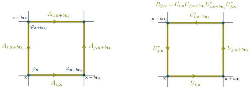
Figure 1: A visual representation of our spatial discretization scheme. Here $b=\Delta x$. The fields $\varphi$ live on the lattice nodes, whereas the gauge fields ${\bf A}$ live on the links.

2.2.1 Lattice action and Hamiltonian

The links and the plaquettes from Eq. (2.29) can be used to define spatial derivates on the lattice (no summation is assumed over repeated indices)

$$(\mathcal{D}_{j}\varphi)_{(\textbf{x})}\rightarrow\frac{U_{j,\textbf{x}}\varphi_{\textbf{x}+\textbf{n}_{j}b}-\varphi_{\textbf{x}}}{b}\,,\quad(F_{ij}F^{ij})_{(\textbf{x})}\rightarrow\frac{2-P_{ij,\textbf{x}}-P_{ji,\textbf{x}}}{b^{4}}\,.$$ (2.30)

Hence, the lattice version of the continuous action from Eq. (2.12) becomes

$$S_{0}^{\rm latt} =\int d\tau\,L_{0}^{\rm latt}$$ (2.31)

$$=\int d\tau\Bigg{\{}-3m_{\mbox{\tiny{Pl}}}^{2}a^{\prime 2}N^{3}+\sum_{\textbf{x}}^{N^{3}}\Bigg{(}\frac{(a\varphi_{1,\textbf{x}}^{\prime})^{2}}{2}+\frac{(a\varphi_{2,\textbf{x}}^{\prime})^{2}}{2}-a^{4}V_{\textbf{x}}+\frac{1}{2e^{2}}\sum_{j}^{1,2,3}A_{j,\textbf{x}}^{\prime 2}$$

$$\qquad-\frac{1}{2e^{2}b^{4}}\sum_{i,j}^{1,2,3}\left[1-P_{ij,\textbf{x}}\right]-\frac{a^{2}}{2b^{2}}\sum_{j}^{1,2,3}\bigg{[}(\varphi_{1,\textbf{x}+\textbf{n}_{j}b}^{2}+\varphi_{2,\textbf{x}+\textbf{n}_{j}b}^{2})+(\varphi_{1,\textbf{x}}^{2}+\varphi_{2,\textbf{x}}^{2})$$

$$\qquad-\left((\varphi_{1,\textbf{x}}-i\varphi_{2,\textbf{x}})U_{j,\textbf{x}}(\varphi_{1,\textbf{x}+\textbf{n}_{j}b}+i\varphi_{2,\textbf{x}+\textbf{n}_{j}b})+{\rm c.c.}\right)\bigg{]}\Bigg{)}\Bigg{\}}\,,$$

where “c.c” refers to complex conjugate. Notice that the three-dimensional integral over space has become a summation over the lattice points $\int d^{3}x\rightarrow\sum_{\textbf{x}}^{N^{3}}b^{3}$, and that the action has been rescaled by a factor of $b^{3}$ – a rescaling of the total action has no effect on the Euler-Lagrange or Hamilton’s equations of motions. The continuous system of five fields capturing infinitely many degrees of freedom and the scale factor has now become one having $5\times N^{3}+1$ generalized coordinates, with conjugate momenta (c.f. (2.16))

$$\pi_{1,\textbf{x}}=a^{2}\varphi_{1,\textbf{x}}^{\prime}\,,\quad\pi_{2,\textbf{x}}=a^{2}\varphi_{2,\textbf{x}}^{\prime}\,,\quad\pi_{\!Aj,\textbf{x}}=e^{-2}A_{j,\textbf{x}}^{\prime}\,,\quad\pi_{a}=-6m_{\mbox{\tiny{Pl}}}^{2}a^{\prime}N^{3}\,.$$ (2.32)

The Legendre transformation yields the lattice Hamiltonian (c.f. (2.17))

$$H_{0}^{\rm latt}(\tau) =\pi_{a}a^{\prime}+\sum_{\textbf{x}}^{N^{3}}\left[\pi_{1}\varphi_{1,\textbf{x}}^{\prime}+\pi_{2}\varphi_{2,\textbf{x}}^{\prime}+\sum_{j}^{1,2,3}\pi_{\!Aj,\textbf{x}}A_{j,\textbf{x}}^{\prime}\right]-L_{0}^{\rm latt}(\tau)$$ (2.33)

$$=-\frac{\pi_{a}^{2}}{12m_{\mbox{\tiny{Pl}}}^{2}N^{3}}+\sum_{\textbf{x}}^{N^{3}}\Bigg{\{}\frac{\pi_{1,\textbf{x}}^{2}}{2a^{2}}+\frac{\pi_{2,\textbf{x}}^{2}}{2a^{2}}+e^{2}\sum_{j}^{1,2,3}\frac{\pi_{Aj,\textbf{x}}^{2}}{2}+\frac{1}{2e^{2}b^{4}}\sum_{i,j}^{1,2,3}\left[1-P_{ij,\textbf{x}}\right]$$

$$\qquad\qquad\qquad+a^{4}V_{\textbf{x}}+\frac{a^{2}}{2b^{2}}\sum_{j}^{1,2,3}\bigg{[}(\varphi_{1,\textbf{x}+\textbf{n}_{j}b}^{2}+\varphi_{2,\textbf{x}+\textbf{n}_{j}b}^{2})+(\varphi_{1,\textbf{x}}^{2}+\varphi_{2,\textbf{x}}^{2})$$

$$\qquad\qquad\qquad-\bigg{(}(\varphi_{1,\textbf{x}}-i\varphi_{2,\textbf{x}})U_{j,\textbf{x}}(\varphi_{1,\textbf{x}+\textbf{n}_{j}b}+i\varphi_{2,\textbf{x}+\textbf{n}_{j}b})+c.c.\bigg{)}\bigg{]}\Bigg{\}}\,.$$

2.2.2 Hamilton’s equations

To extremise the lattice action in Eq. (2.31) we need to use the corresponding Hamilton’s equations. We can again write them concisely in terms of the lattice Poisson brackets (c.f. (2.18))

$$\{\mathcal{A}_{\textbf{x}^{\prime}},\mathcal{B}_{\textbf{x}^{\prime\prime}}\}^{\rm latt}_{\rm P}\equiv\frac{\partial\mathcal{A}_{\textbf{x}^{\prime}}}{\partial a}\frac{\partial\mathcal{B}_{\textbf{x}^{\prime\prime}}}{\partial\pi_{a}}-\frac{\partial\mathcal{B}_{\textbf{x}^{\prime\prime}}}{\partial a}\frac{\partial\mathcal{A}_{\textbf{x}^{\prime}}}{\partial\pi_{a}}+\sum_{\textbf{x}}^{N^{3}}\sum_{i=1}^{5}\left[\frac{\partial\mathcal{A}_{\textbf{x}^{\prime}}}{\partial Q_{\textbf{x},i}}\frac{\partial\mathcal{B}_{\textbf{x}^{\prime\prime}}}{\partial P_{\textbf{x},i}}-\frac{\partial\mathcal{B}_{\textbf{x}^{\prime\prime}}}{\partial Q_{\textbf{x},i}}\frac{\partial\mathcal{A}_{\textbf{x}^{\prime}}}{\partial P_{\textbf{x},i}}\right]\,,$$ (2.34)

where $Q_{\textbf{x}}=[\varphi_{1,\textbf{x}},\varphi_{2,\textbf{x}},A_{1,\textbf{x}},A_{2,\textbf{x}},A_{3,\textbf{x}}]^{T}$, $P_{\textbf{x}}=[\pi_{1,\textbf{x}},\pi_{2,\textbf{x}},\pi_{A1,\textbf{x}},\pi_{A2,\textbf{x}},\pi_{A3,\textbf{x}}]^{T}$ and all quantities are evaluated at equal times. $\mathcal{A}$ and $\mathcal{B}$ are functions of the lattice fields and lattice momenta, i.e.,

$$\mathcal{A}_{\textbf{x}} \equiv\mathcal{A}(a,Q_{\textbf{x},i},\pi_{a},P_{\textbf{x},i})\,,$$ (2.35)

$$\mathcal{B}_{\textbf{x}} \equiv\mathcal{B}(a,Q_{\textbf{x},i},\pi_{a},P_{\textbf{x},i})\,.$$

The lattice Hamilton’s equations can be now expressed as

$$\partial_{\tau}a =\left\{a,H_{0}^{\rm latt}\right\}_{\rm P}^{\rm latt}\,,$$ (2.36)

$$\partial_{\tau}\pi_{a} =\left\{p_{a},H_{0}^{\rm latt}\right\}_{\rm P}^{\rm latt}\,,$$

$$\partial_{\tau}Q_{\textbf{x},i} =\left\{Q_{\textbf{x},i},H_{0}^{\rm latt}\right\}_{\rm P}^{\rm latt}\,,$$

$$\partial_{\tau}P_{\textbf{x},i} =\left\{P_{\textbf{x},i},H_{0}^{\rm latt}\right\}_{\rm P}^{\rm latt}\,,$$

where again the first and third lines are the definitions of the lattice conjugate momenta from Eq. (2.32), whilst the second and fourth lines are the evolution equations for the scale factor and the lattice fields, respectively. We are again missing the (lattice version of the) Gauss constraint. Just like before, it can be recovered from a residual gauge symmetry of the lattice action, Eq. (2.31), as we show in the following section.

2.2.3 Gauss constraint

Thanks to the links and plaquettes the lattice action given in Eq. (2.31) is invariant under the time-independent symmetry transformations

$$\varphi_{\textbf{x}}\rightarrow\Omega_{\textbf{x}}\varphi_{\textbf{x}}\,,\quad U_{j,\textbf{x}}\rightarrow\Omega_{\textbf{x}}U_{j,\textbf{x}}\Omega_{\textbf{x}+\textbf{n}_{j}b}^{*}\,\quad{\rm where}\quad\Omega_{\textbf{x}}=\exp[-i\alpha_{\textbf{x}}]\,.$$ (2.37)

In their infinitesimal form ($\alpha_{\textbf{x}}\ll 1$),

$$\delta\varphi_{1,\textbf{x}}=\varphi_{2,\textbf{x}}\alpha_{\textbf{x}}\,,\quad\delta\varphi_{2,\textbf{x}}=-\varphi_{1,\textbf{x}}\alpha_{\textbf{x}}\,,\quad\delta A_{j,\textbf{x}}=\frac{\alpha_{\textbf{x}+\textbf{n}_{j}b}-\alpha_{\textbf{x}}}{b}\,.$$ (2.38)

The Noether theorem then implies that for arbitrary $\alpha_{\textbf{x}}$, there is a conserved charge

$$J(\tau) =\sum_{\textbf{x}}^{N^{3}}\sum_{i=1}^{5}\frac{\partial L_{0}^{\rm latt}}{\partial Q^{\prime}_{\textbf{x},i}}\delta Q_{\textbf{x},i}$$ (2.39)

$$=\sum_{\textbf{x}}^{N^{3}}\left[\alpha_{\textbf{x}}(\pi_{1,\textbf{x}}(\tau)\varphi_{2,\textbf{x}}(\tau)-\pi_{2,\textbf{x}}(\tau)\varphi_{1,\textbf{x}}(\tau))+\sum_{j}^{1,2,3}\pi_{Aj,\textbf{x}}(\tau)\frac{\alpha_{\textbf{x}+\textbf{n}_{j}b}-\alpha_{\textbf{x}}}{b}\right]$$

$$=\text{const}\,.$$

It reduces to

$$J(\tau)=\sum_{\textbf{x}}^{N^{3}}\alpha_{\textbf{x}}\left[\left(\pi_{1,\textbf{x}}(\tau)\varphi_{2,\textbf{x}}(\tau)-\pi_{2,\textbf{x}}(\tau)\varphi_{1,\textbf{x}}(\tau)\right)-\sum_{j}^{1,2,3}\frac{\pi_{Aj,\textbf{x}}(\tau)-\pi_{Aj,\textbf{x}-\textbf{n}_{j}b}(\tau)}{b}\right]=\text{const}\,.$$ (2.40)

Note that $J^{\prime}(\tau)=0$ holds for arbitrary $\alpha_{\textbf{x}}$. Hence, at each lattice point

$$e^{-2}\mathcal{C}_{\rm G,\textbf{x}}^{\rm latt}(\tau)=\sum_{j}^{1,2,3}\left[\frac{\pi_{Aj,\textbf{x}}(\tau)-\pi_{Aj,\textbf{x}-\textbf{n}_{j}b}(\tau)}{b}\right]-\left(\pi_{1,\textbf{x}}(\tau)\varphi_{2,\textbf{x}}(\tau)-\pi_{2,\textbf{x}}(\tau)\varphi_{1,\textbf{x}}(\tau)\right)=\text{const}\,.$$ (2.41)

This is the lattice counterpart to the Gauss constraint given in Eq. (2.26). Thus, the gauge-fixed lattice action, Eq. (2.31), again enforces $\partial_{\tau}\mathcal{C}_{\rm G,\textbf{x}}^{\rm latt}=0$ and so do its Hamilton’s equations. The desired Abelian-Higgs theory with $\mathcal{C}_{\rm G,\textbf{x}}^{\rm latt}(\tau)=0$ is recovered by imposing the Gauss constraint on the initial conditions and then using the lattice Hamilton’s equations to evolve the system.

The remaining question is whether there is a way to discretize in time the lattice fields, so that their evolution (according to the corresponding discretized in time lattice Hamilton’s equations) still respects the Gauss constraint in Eq. (2.41). We show in the next section, that there is a scheme based on symplectic discretization which does that.

3 GFiRe implementation

As we argue below, we can numerically time-evolve the Abelian-Higgs system prescribed by the lattice action in (2.31) and meet the Gauss constraint (2.41) everywhere on the lattice using symplectic integrators.

In ${\sf GFiRe}$, we use a symplectic prescription to integrate the Hamilton’s equations on the lattice (Eqns. (2.36)), which we write compactly as

$$z_{j}^{\prime}(\tau) =\left\{z_{j}(\tau),H_{0}^{\rm latt}\Big{(}z_{j}(\tau)\Big{)}\right\}_{\rm P}^{\rm latt}\,,$$ (3.1)

where $z=[a,\varphi_{1,\textbf{x}},\varphi_{2,\textbf{x}},A_{1,\textbf{x}},A_{2,\textbf{x}},A_{3,\textbf{x}},p_{a},\pi_{1,\textbf{x}},\pi_{2,\textbf{x}},\pi_{A1,\textbf{x}},\pi_{A2,\textbf{x}},\pi_{A3,\textbf{x}}]^{T}$, i.e., the integer $j$ index of $z$ runs over the $2\times\left(1+5\times N^{3}\right)$ phase space variables. In the rest of the section we give the details of the numerical integrator.

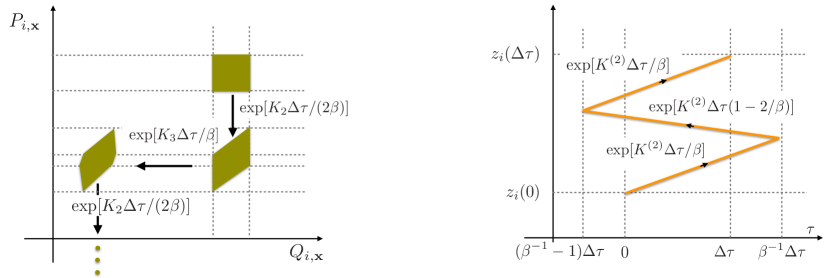
Figure 2: A visual representation our composite symplectic time integrator. The left panel shows the symplectic nature of the integrator, whereas the right panel describes the composition of the building block of the symplectic integrator.

3.1 Symplectic integrators

We first present the structure of the symplectic integrator used by ${\sf GFiRe}$ in an abstract form. It might be useful to refer to Fig. 2 for a schematic picture of the integrator.

We need two assumptions about the form of the Hamiltonian. First, we assume that the Hamiltonian splits into three mutually non-commuting terms

$$H=H_{1}+H_{2}+H_{3}\,,$$ (3.2)

$$\left\{H_{i},H_{j}\right\}_{{}_{\text{P}}}\neq 0\,.$$

Second, we also assume that each Hamiltonian term is a function of only one variable from each pair of generalized coordinate and corresponding conjugate momentum. In other words, for a given $j$ we have either $\partial H_{i}/\partial q_{j}=0$ or $\partial H_{i}/\partial p_{j}=0$ or both (here $p_{j}$ is the conjugate momentum to the generalised coordinate $q_{j}$). This assumption allows us to use standard symplectic integrator techniques [107].

The formal solution to the Hamilton’s equations (3.1), can be written as

$$z_{j}(\tau+\Delta\tau)=\exp[\left\{\cdot,H\right\}_{{}_{\text{P}}}\Delta\tau]z_{j}(\tau)\,,$$ (3.3)

for an arbitrary time interval $\Delta\tau$. The numerical approximation for any finite time interval $\Delta\tau$ is (see [107]):

$$z_{j}(\tau+\Delta\tau)=\exp[K^{(k)}\Delta\tau]z_{j}(\tau)\,,$$ (3.4)

where $\Delta\tau$ is the time step and $K^{(k)}$ is an operator involving Poisson brackets with the Hamiltonian terms from Eq. (LABEL:eq:HamiltonSpli). The choice of the integrator order, $k$, determines the exact form of the operator. Thanks to our two assumptions, we can use a symplectic method of integration based on operator splitting techniques [107]. The integrator of lowest order, $k=2$, is

$$\exp[K^{(2)}\Delta\tau] \equiv\exp[K_{1}\Delta\tau/2]\exp[K_{2}\Delta\tau/2]\exp[K_{3}\Delta\tau]\exp[K_{2}\Delta\tau/2]\exp[K_{1}\Delta\tau/2]$$ (3.5)

$$=\exp[\{\cdot,H\}_{{}_{\text{P}}}\Delta\tau]+\mathcal{O}(\Delta\tau^{3})\,,$$

$$K_{i} =\{\cdot,H_{i}\}_{{}_{\text{P}}}\,,$$

whereas higher-order operators are obtained recursively

$$\exp[K^{(k+2)}\Delta\tau] \equiv\exp[K^{(k)}\Delta\tau/\beta]\exp[K^{(k)}\Delta\tau(1-2\beta^{-1})]\exp[K^{(k)}\Delta\tau/\beta]$$ (3.6)

$$=\exp[\{\cdot,H\}_{{}_{\text{P}}}\Delta\tau]+\mathcal{O}(\Delta\tau^{k+3})\,,$$

$$\beta =2-2^{1/(k+1)}\,.$$

The numerical solution can be made arbitrarily close to the true one as one increases $k$ and/or decreases $\Delta\tau$. Hence, an integrator of arbitrary accuracy has been reduced to the operation of $\exp[K_{1}\Delta\tau]$, $\exp[K_{2}\Delta\tau]$ and $\exp[K_{3}\Delta\tau]$ in some particular combination and taking the appropriate values for the time interval $\Delta\tau$ for each operation. Let’s see how this can be implemented for the Abelian-Higgs system.

3.2 Evolution on the lattice

The lattice Hamiltonian, $H_{0}^{\rm latt}$, from Eq. (2.33), splits into three non-commuting terms, just like in Eq. (LABEL:eq:HamiltonSpli),

$$H_{0}^{\rm latt}=H_{1}+H_{2}+H_{3}\,,$$ (3.7)

$$H_{1}=-\frac{\pi_{a}^{2}}{12m_{\mbox{\tiny{Pl}}}^{2}N^{3}}\,,\qquad H_{2}=\sum_{\textbf{x}}^{N^{3}}\left[\frac{\pi_{1,\textbf{x}}^{2}}{2a^{2}}+\frac{\pi_{2,\textbf{x}}^{2}}{2a^{2}}+e^{2}\sum_{j}^{1,2,3}\frac{\pi_{Aj,\textbf{x}}^{2}}{2}\right]\,,$$

$$H_{3}=\sum_{\textbf{x}}^{N^{3}}\Bigg{\{}a^{4}V_{\textbf{x}}+\frac{1}{2e^{2}b^{4}}\sum_{i,j}^{1,2,3}\left[1-P_{ij,\textbf{x}}\right]+\frac{a^{2}}{2b^{2}}\sum_{j}^{1,2,3}\bigg{[}(\varphi_{1,\textbf{x}+\textbf{n}_{j}b}^{2}+\varphi_{2,\textbf{x}+\textbf{n}_{j}b}^{2})$$

$$\qquad\qquad+(\varphi_{1,\textbf{x}}^{2}+\varphi_{2,\textbf{x}}^{2})-\bigg{(}(\varphi_{1,\textbf{x}}-i\varphi_{2,\textbf{x}})U_{j,\textbf{x}}(\varphi_{1,\textbf{x}+\textbf{n}_{j}b}+i\varphi_{2,\textbf{x}+\textbf{n}_{j}b})+c.c.\bigg{)}\bigg{]}\Bigg{\}}\,.$$

Note that each of the terms is a function either of a generalised coordinate or its conjugate momentum, but never of both consistent with our second assumption in the previous, more formal subsection.

We can now use Eqs. (3.4), (3.5) and (3.6) to evolve the complex scalar, 3-vector gauge field, scale factor and their conjugate momenta. To this end we must find the action of each $\exp[K_{i}\Delta\tau]$ on the lattice phase space variables. In deriving the expressions below, we make an extensive use of the operator identity for our Hamiltonian (2.33):

$$\exp[K_{i}\Delta\tau]z_{j}=(1+K_{i}\Delta\tau)z_{j}\,,$$ (3.8)

when applied to any $z_{j}$. Note that this is not an approximation in the context of our Hamiltonian.

After acting with $\exp[K_{1}\Delta\tau/2]$ on all $z_{j}$ we get (see Eq. (3.4))

$$a\rightarrow a-\left(\frac{\Delta\tau}{2}\right)\frac{\pi_{a}}{6m_{\mbox{\tiny{Pl}}}^{2}N^{3}}\,,$$ (3.9)

with the rest of $z_{j}$ unchanged. Similarly, the action of $\exp[K_{2}\Delta\tau/2]$ yields

$$\varphi_{1,\textbf{x}} \rightarrow\varphi_{1,\textbf{x}}+\left(\frac{\Delta\tau}{2}\right)\frac{\pi_{1,\textbf{x}}}{a^{2}}\,,\quad\varphi_{2,\textbf{x}}\rightarrow\varphi_{2,\textbf{x}}+\left(\frac{\Delta\tau}{2}\right)\frac{\pi_{2,\textbf{x}}}{a^{2}}\,,$$ (3.10)

$$A_{j,\textbf{x}} \rightarrow A_{j,\textbf{x}}+\left(\frac{\Delta\tau}{2}\right)e^{2}\pi_{Aj,\textbf{x}}\,,\quad\pi_{a}\rightarrow\pi_{a}+\left(\frac{\Delta\tau}{2}\right)\sum_{\textbf{x}}^{N^{3}}\left[\frac{\pi_{1,\textbf{x}}^{2}}{a^{3}}+\frac{\pi_{2,\textbf{x}}^{2}}{a^{3}}\right]\,,$$

leaving the rest of the generalized coordinates and momenta unchanged. Finally, the action of $\exp[K_{3}\Delta\tau]$ gives

$$\pi_{1,\textbf{x}} \rightarrow\pi_{1,\textbf{x}}+\Delta\tau\Bigg{\{}-a^{4}\frac{\partial V_{\textbf{x}}}{\partial\varphi_{1,\textbf{x}}}-\frac{6a^{2}\varphi_{1,\textbf{x}}}{b^{2}}+\frac{a^{2}}{2b^{2}}\sum_{j}^{1,2,3}\Bigg{[}U_{j,\textbf{x}}(\varphi_{1,\textbf{x}+\textbf{n}_{j}b}+i\varphi_{2,\textbf{x}+\textbf{n}_{j}b})$$ (3.11)

$$\qquad\qquad\qquad\qquad\qquad\qquad\qquad\qquad\qquad+(\varphi_{1,\textbf{x}-\textbf{n}_{j}b}-i\varphi_{2,\textbf{x}-\textbf{n}_{j}b})U_{j,\textbf{x}-\textbf{n}_{j}b}+c.c.\Bigg{]}\Bigg{\}}\,,$$

$$\pi_{2,\textbf{x}} \rightarrow\pi_{2,\textbf{x}}+\Delta\tau\Bigg{\{}-a^{4}\frac{\partial V_{\textbf{x}}}{\partial\varphi_{2,\textbf{x}}}-\frac{6a^{2}\varphi_{2,\textbf{x}}}{b^{2}}+\frac{a^{2}}{2b^{2}}\sum_{j}^{1,2,3}\Bigg{[}-iU_{j,\textbf{x}}(\varphi_{1,\textbf{x}+\textbf{n}_{j}b}+i\varphi_{2,\textbf{x}+\textbf{n}_{j}b})$$

$$\qquad\qquad\qquad\qquad\qquad\qquad\qquad\qquad\qquad+i(\varphi_{1,\textbf{x}-\textbf{n}_{j}b}-i\varphi_{2,\textbf{x}-\textbf{n}_{j}b})U_{j,\textbf{x}-\textbf{n}_{j}b}+c.c.\Bigg{]}\Bigg{\}}\,,$$

$$\pi_{Aj,\textbf{x}} \rightarrow\pi_{Aj,\textbf{x}}+\Delta\tau\Bigg{\{}\frac{a^{2}}{2b}\left[i(\varphi_{1,\textbf{x}}-i\varphi_{2,\textbf{x}})U_{j,\textbf{x}}(\varphi_{1,\textbf{x}+\textbf{n}_{j}b}+i\varphi_{2,\textbf{x}+\textbf{n}_{j}b})+c.c.\right]$$

$$\qquad\qquad\qquad\qquad\qquad\qquad\qquad\qquad\qquad+\frac{1}{2e^{2}b^{3}}\sum_{l}^{1,2,3}\left[iP_{jl,\textbf{x}}+iP_{lj,\textbf{x}-\textbf{n}_{l}b}+c.c.\right]\Bigg{\}}\,,$$

$$\pi_{a} \rightarrow\pi_{a}+\Delta\tau\sum_{\textbf{x}}^{N^{3}}\Bigg{\{}-4a^{3}V_{\textbf{x}}-\frac{a}{b^{2}}\sum_{j}^{1,2,3}\bigg{[}(\varphi_{1,\textbf{x}+\textbf{n}_{j}b}^{2}+\varphi_{2,\textbf{x}+\textbf{n}_{j}b}^{2})+(\varphi_{1,\textbf{x}}^{2}+\varphi_{2,\textbf{x}}^{2})$$

$$\qquad\qquad\qquad\qquad\qquad\qquad-\bigg{(}(\varphi_{1,\textbf{x}}-i\varphi_{2,\textbf{x}})U_{j,\textbf{x}}(\varphi_{1,\textbf{x}+\textbf{n}_{j}b}+i\varphi_{2,\textbf{x}+\textbf{n}_{j}b})+c.c.\bigg{)}\bigg{]}\Bigg{\}}\,,$$

with no changes in the generalised coordinates. Below, we state one of the main benefits of using the above scheme for time evolution.

3.3 Preservation of the Gauss constraint

We verify explicitly that after each individual step, Eq. (3.9) and/or Eq. (3.10) and/or Eq. (3.11), the lattice Gauss constraint, Eq. (2.41), is respected exactly, $\mathcal{C}_{\rm G,\textbf{x}}^{\rm latt}(\tau)=\text{const}$.

To see this, first note that the action of $\exp[K_{1}\Delta\tau/2]$ (see Eq. (3.9)) trivially yields $\mathcal{C}_{\rm G,\textbf{x}}^{\rm latt}\rightarrow\mathcal{C}_{\rm G,\textbf{x}}^{\rm latt}$. The $\exp[K_{2}\Delta\tau/2]$ step (see Eq. (3.10)) gives

$$\mathcal{C}_{\rm G,\textbf{x}}^{\rm latt}\rightarrow\mathcal{C}_{\rm G,\textbf{x}}^{\rm latt}-e^{2}\left[\pi_{1,\textbf{x}}\left(\frac{\Delta\tau}{2}\right)\frac{\pi_{2,\textbf{x}}}{a^{2}}-\pi_{2,\textbf{x}}\left(\frac{\Delta\tau}{2}\right)\frac{\pi_{1,\textbf{x}}}{a^{2}}\right]=\mathcal{C}_{\rm G,\textbf{x}}^{\rm latt}\,.$$ (3.12)

Finally, the $\exp[K_{3}\Delta\tau]$ (see Eq. (3.11)) operation yields

$$\mathcal{C}_{\rm G,\textbf{x}}^{\rm latt} \rightarrow\mathcal{C}_{\rm G,\textbf{x}}^{\rm latt}+\frac{e^{2}}{b}\sum_{j}^{1,2,3}\Delta\tau\Bigg{\{}\frac{a^{2}}{2b}\left[i(\varphi_{1,\textbf{x}}-i\varphi_{2,\textbf{x}})U_{j,\textbf{x}}(\varphi_{1,\textbf{x}+\textbf{n}_{j}b}+i\varphi_{2,\textbf{x}+\textbf{n}_{j}b})+c.c.\right]$$ (3.13)

$$\qquad\qquad\qquad\qquad\qquad\qquad\qquad\qquad+\frac{1}{2e^{2}b^{3}}\sum_{l}^{1,2,3}\left[iP_{jl,\textbf{x}}+iP_{lj,\textbf{x}-\textbf{n}_{l}b}+c.c.\right]\Bigg{\}}$$

$$-\frac{e^{2}}{b}\sum_{j}^{1,2,3}\Delta\tau\Bigg{\{}\frac{a^{2}}{2b}\left[i(\varphi_{1,\textbf{x}-\textbf{n}_{j}b}-i\varphi_{2,\textbf{x}-\textbf{n}_{j}b})U_{j,\textbf{x}-\textbf{n}_{j}b}(\varphi_{1,\textbf{x}}+i\varphi_{2,\textbf{x}})+c.c.\right]$$

$$\qquad\qquad\qquad\qquad\qquad\qquad+\frac{1}{2e^{2}b^{3}}\sum_{l}^{1,2,3}\left[iP_{jl,\textbf{x}-\textbf{n}_{j}b}+iP_{lj,\textbf{x}-\textbf{n}_{j}b-\textbf{n}_{l}b}+c.c.\right]\Bigg{\}}$$

$$-e^{2}\varphi_{2,\textbf{x}}\Delta\tau\Bigg{\{}-a^{4}\frac{\partial V_{\textbf{x}}}{\partial\varphi_{1,\textbf{x}}}-\frac{6a^{2}\varphi_{1,\textbf{x}}}{b^{2}}+\frac{a^{2}}{2b^{2}}\sum_{j}^{1,2,3}\Bigg{[}U_{j,\textbf{x}}(\varphi_{1,\textbf{x}+\textbf{n}_{j}b}+i\varphi_{2,\textbf{x}+\textbf{n}_{j}b})$$

$$\qquad\qquad\qquad\qquad\qquad\quad\qquad\qquad+(\varphi_{1,\textbf{x}-\textbf{n}_{j}b}-i\varphi_{2,\textbf{x}-\textbf{n}_{j}b})U_{j,\textbf{x}-\textbf{n}_{j}b}+c.c.\Bigg{]}\Bigg{\}}$$

$$+e^{2}\varphi_{1,\textbf{x}}\Delta\tau\Bigg{\{}-a^{4}\frac{\partial V_{\textbf{x}}}{\partial\varphi_{2,\textbf{x}}}-\frac{6a^{2}\varphi_{2,\textbf{x}}}{b^{2}}+\frac{a^{2}}{2b^{2}}\sum_{j}^{1,2,3}\Bigg{[}-iU_{j,\textbf{x}}(\varphi_{1,\textbf{x}+\textbf{n}_{j}b}+i\varphi_{2,\textbf{x}+\textbf{n}_{j}b})$$

$$\qquad\qquad\qquad\qquad\qquad\qquad\quad\qquad+i(\varphi_{1,\textbf{x}-\textbf{n}_{j}b}-i\varphi_{2,\textbf{x}-\textbf{n}_{j}b})U_{j,\textbf{x}-\textbf{n}_{j}b}+c.c.\Bigg{]}\Bigg{\}}$$

$$=\mathcal{C}_{\rm G,\textbf{x}}^{\rm latt}\,,$$

where the $\partial V$ terms cancel due to the $U(1)$ symmetry of the potential, the links, $U_{j}$, terms in the first two big brackets cancel with the links terms in the other two big brackets, whereas the sums of the Plaquette terms vanish by virtue of the identity $\sum_{j,l}^{1,2,3}\Big{[}iP_{jl,\textbf{x}}+c.c.\Big{]}=0$. (also see Eq. (2.29)).

Another, perhaps more impressive way of stating our result is that when we evaluate $\mathcal{C}^{\rm latt}_{G}$ at $\tau+\Delta\tau$ by using the above expressions for time evolved $z_{j}$, all terms proportional to $\Delta\tau^{n}$ for arbitrary $n$ vanish. Thus, regardless of the order of the time integrator, k, the Gauss constraint is always satisfied to machine precision at each lattice site. As we showed above, for physical consistency, initially we must set the constant on the right hand side in the Gauss constraint equation, Eq. (2.41), to zero everywhere on the lattice. The symplectic evolution now guarantees that it remains zero at later times.

3.4 Approximate post-inflationary initial conditions

Within the inflationary paradigm, the (almost) homogeneous inflaton field dominates the Universe during and shortly after the end of inflation. One can assume that the inflaton is the real part of the complex salar (i.e., slow-roll inflation is realized along the real axis in the complex field space, towards the minimum of the scalar field potential, see Fig. 3). At the beginning of our simulations of preheating, the initial variables on the lattice are

$$\varphi_{1,\textbf{x}}=\bar{\varphi}_{1}+\delta\varphi_{1,\textbf{x}}\,,\quad\varphi_{2,\textbf{x}}=\delta\varphi_{2,\textbf{x}}\,,\quad\pi_{1,\textbf{x}}=\bar{\pi}_{1}+\delta\pi_{1,\textbf{x}}\,,\quad\pi_{2,\textbf{x}}=\delta\pi_{2,\textbf{x}}\,,$$ (3.14)

$$A_{j,\textbf{x}}=\delta A_{j,\textbf{x}}\,,\quad\pi_{Aj,\textbf{x}}=\delta\pi_{Aj,\textbf{x}}\,,\quad a=1\,,\quad\pi_{a}=-2\sqrt{3}m_{\mbox{\tiny{Pl}}}N^{3}\sqrt{\frac{H_{2}+H_{3}}{N^{3}}}\,,$$

where the choice for the initial value of $a$ is conventional and the expression for $\pi_{a}$ is simply the Friedmann equation. At later times, we use this expression to check the ‘energy conservation’ of our integrators. We observe violations that scale correctly with the time step – $\mathcal{O}(\Delta\tau^{k})$ for k-th order integrators. The $\bar{\varphi}_{1}$ and $\bar{\pi}_{1}$ variables are determined from the homogeneous inflationary dynamics, whereas the $\delta$-field perturbations have a power spectrum set by the quantum vacuum fluctuations.

The initial fluctuations for each lattice field can be expanded in terms of Fourier modes. These can be then written in terms of products of mode functions and ‘stochastic’ complex numbers. The stochasticity in the initial field perturbations is what allows the classical simulations to approximately capture aspects of the quantum uncertainty in the actual vacuum fluctuations. We also must satisfy the Gauss constraint, Eq. (2.41), with the constant term

$$\delta\varphi_{1,\textbf{x}} =\frac{(2\pi)^{3/2}}{L^{3/2}_{\text{lat}}}\sum_{\textbf{k}}e^{i\textbf{k}\cdot\textbf{x}}\delta\varphi_{1,\textbf{k}}=\frac{(2\pi)^{3/2}}{L^{3/2}_{\text{lat}}}\sum_{\textbf{k}}e^{i\textbf{k}\cdot\textbf{x}}\Big{[}a_{\textbf{k}}^{1}u_{k}^{1}+a_{-\textbf{k}}^{1*}u_{k}^{1*}\Big{]}\,,$$ (3.16)

$$\delta\pi_{1,\textbf{x}} =\frac{(2\pi)^{3/2}}{L^{3/2}_{\text{lat}}}\sum_{\textbf{k}}e^{i\textbf{k}\cdot\textbf{x}}\delta\pi_{1,\textbf{k}}=\frac{(2\pi)^{3/2}}{L^{3/2}_{\text{lat}}}\sum_{\textbf{k}}e^{i\textbf{k}\cdot\textbf{x}}\Big{[}a_{\textbf{k}}^{1}{u_{k}^{1}}^{\prime}+a_{-\textbf{k}}^{1*}{u_{k}^{1*}}^{\prime}\Big{]}\,,$$

$$\delta\varphi_{2,\textbf{x}} =\frac{(2\pi)^{3/2}}{L^{3/2}_{\text{lat}}}\sum_{\textbf{k}}e^{i\textbf{k}\cdot\textbf{x}}\delta\varphi_{2,\textbf{k}}=\frac{(2\pi)^{3/2}}{L^{3/2}_{\text{lat}}}\sum_{\textbf{k}}e^{i\textbf{k}\cdot\textbf{x}}\Big{[}a_{\textbf{k}}^{2}u_{k}^{2}+a_{-\textbf{k}}^{2*}u_{k}^{2*}\Big{]}\,,$$

$$\delta\pi_{2,\textbf{x}} =\delta\varphi_{2,\textbf{x}}\frac{\bar{\pi}_{1}+\delta\pi_{1,\textbf{x}}}{\bar{\varphi}_{1}+\delta\varphi_{1,\textbf{x}}}\,,$$

$$A_{j,\textbf{x}} =\frac{(2\pi)^{3/2}}{L^{3/2}_{\text{lat}}}\sum_{\textbf{k}}e^{i\textbf{k}\cdot\textbf{x}}A_{j\textbf{k}}=\frac{(2\pi)^{3/2}}{L^{3/2}_{\text{lat}}}\sum_{\textbf{k}}e^{i\textbf{k}\cdot\textbf{x}}\Big{[}a_{\textbf{k}}^{Aj}u_{k}^{Aj}+\left(a_{-\textbf{k}}^{Aj}u_{k}^{Aj}\right)^{*}\Big{]}\,,$$

$$\pi_{Aj,\textbf{x}} =0\,.$$

The random (‘stochastic’) complex numbers provide the classical counterpart of the quantum creation and annihilation operators, and take the values

$$\left|a_{\textbf{k}}^{I}\right|=\sqrt{-\ln\left(X_{\textbf{k}}^{I}\right)/2}\,,\quad\text{arg}\left(a_{\textbf{k}}^{I}\right)=2\pi Y_{\textbf{k}}^{I}\,.$$ (3.17)

Here $X_{\textbf{k}}^{I}$ is a uniform deviate on $(0,1)$ and $Y_{\textbf{k}}^{I}$ is a uniform deviate on $[0,1)$. The mode functions are given by the flat spacetime expressions

$$u^{1}_{k} =\frac{\exp\left(-i\sqrt{k^{2}+(\partial^{2}/\partial\bar{\varphi}_{1}^{2})V}\tau\right)}{\sqrt{2}\left(k^{2}+(\partial^{2}/\partial\bar{\varphi}_{1}^{2})V\right)^{1/4}}\,,$$ (3.18)

$$u^{2}_{k} =\frac{\exp\left(-i\sqrt{k^{2}+(\partial^{2}/\partial\bar{\varphi}_{2}^{2})V}\tau\right)}{\sqrt{2}\left(k^{2}+(\partial^{2}/\partial\bar{\varphi}_{2}^{2})V\right)^{1/4}}\,,$$

$$u^{Aj}_{k} =\frac{\exp\left(-i\sqrt{k^{2}+k_{\!{}_{C}}^{2}}\tau\right)}{\sqrt{2}(k^{2}+k_{\!{}_{C}}^{2})^{1/4}}\,,$$

which approximate well the modes of interest, i.e., subhorizon modes, $k\gg\mathcal{H}$, at the end of inflation, regardless of the coupling strength, parametrised by the comoving Compton wavenumber, $k_{\!{}_{C}}\equiv e\bar{\varphi}_{1}$, for the gauge fields. Note that the normalization factor of $(2\pi)^{3/2}/L^{3/2}_{\text{lat}}$ in Eq. (3.16) is needed to make the (initial) two-point functions of field perturbations, averaged over the lattice volume, independent of the comoving box size, $L_{\text{lat}}=Nb$, and equal to the continuous ones, see for example, [70].

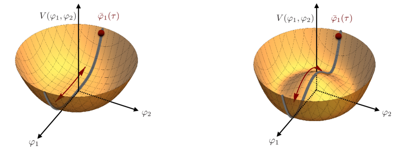
Figure 3: The complex scalar potential profile, see Eq. (4.1), for two separate cases $v=0$ (left panel) and $v\neq 0$ (right panel). After inflation ends, the field is primarily rolling down along $\varphi_{1}$-axis, followed by oscillations about the minimum, which can lead to resonant particle production in the gauge fields as well as the $\varphi$ field. Note that in both cases, we begin with $\bar{\varphi}_{1}(\tau_{\rm in})\gg v$.

4 Numerical studies of the scalar electrodynamics

To test our algorithm, we study the non-linear dynamics in models with the scalar field potential (see Fig. 3)

$$V=\frac{\lambda}{4}\left(\varphi_{1}^{2}+\varphi_{2}^{2}-v^{2}\right)^{2}\,.$$ (4.1)

For concreteness, we assume $\varphi_{1}$ to play the role of the inflaton and set $\lambda=9\times 10^{-14}$. The initial conditions at the start of the simulations (and the end of slow-roll inflation) are of the form given in Section 3.4, with

$$\bar{\varphi}_{1}=\phi_{0}=1.71m_{\mbox{\tiny{Pl}}}\gg v\,.$$ (4.2)

Note that this setup corresponds to the well-known quartic inflationary scenario [110, 111]. As such, this particular shape of the potential is in conflict with CMB observations [112]. Nevertheless, since the main focus of this section is on the post-inflationary dynamics, we content ourselves with interpreting Eq. (4.1) as the effective form of the inflaton potential after inflation, remaining agnostic about the details of $V$ during inflation. For simplicity, we also set $\bar{\pi}_{1}=0$ initially.

Shortly after the end of inflation $\bar{\varphi}_{1}(\tau)$ begins to oscillate. Its oscillations can amplify exponentially fast the initial field fluctuations, $\delta\varphi_{1}$, $\delta\varphi_{2}$ and $\delta\boldsymbol{\rm{A}}$. The phenomenon can be understood in terms of parametric resonance [113] and is more generally known in the context of inflation as preheating [5]. The field fluctuations can grow very quickly, until mode-mode couplings become non-negligible. This marks the end of the linear stage of preheating [9] and the onset of backreaction. The ensuing non-linear dynamics can be quite rich and is strongly dependent on $v$. We now consider two different scenarios – $v=0$ and $v\neq 0$, separately and study the linear and non-linear regimes with our numerical prescription.

For the results below, we typically rely on a $N^{3}=512^{3}$ lattice. We use a fourth order symplectic integrator ($k=2$ in the notation of Eq. (3.6)) with a time step $\Delta\tau=0.028(\sqrt{\lambda}\phi_{0})^{-1}$ and comoving edge length $L_{\rm latt}=60(\sqrt{\lambda}\phi_{0})^{-1}$. The comoving lattice spacing $\Delta x=L_{\rm latt}/N$. Note that we always have $\Delta\tau<\Delta x$. By the end of the simulations $a(\tau_{f})\Delta x<1/(\sqrt{\lambda}v)$ where $\sqrt{\lambda}v$ is the mass scale in the valley of the potential in the $v\neq 0$ case. In the $v=0$ case, the effective inverse mass scale case grows with the scale factor, hence we always resolve the relevant spatial and temporal scales at late times, if we resolve them initially.

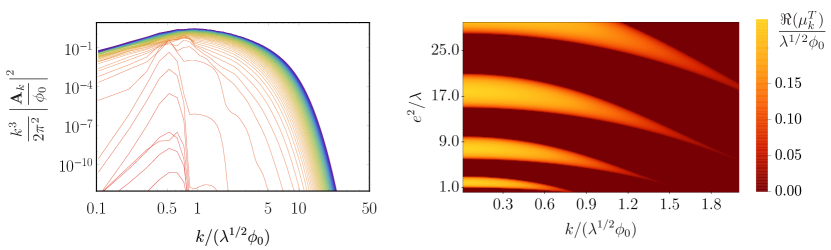
Figure 4: Left panel: The evolution of the gauge field power spectrum for $v=0$, extracted from our lattice simulations. The different colors correspond to different times, going from red to blue. The initial rapid growth of a broad range of comoving momentum, $k$, modes (dark red curves) is a manifestation of resonant particle production. It is eventually shut off by backreaction of the gauge field on the Higgs condensate. At late times the power distribution becomes time-independent. Right panel: The Floquet chart corresponding to the instability in the transverse components of the gauge fields.

4.1 Nonlinear dynamics in the $v=0$ case

We begin with $v=0$, for which the scalar field potential profile takes the form of a quartic bowl, see Fig. 3. At the start of the simulations, the background scalar field oscillates along the real axis in the complex $\varphi$ plane, as shown in the left panel of the figure. Depending on the ratio $e^{2}/\lambda$, these oscillations can lead to the exponential amplification of the complex scalar and/or the gauge field fluctuations. We set

$$e=\sqrt{\lambda}\,.$$ (4.3)

This choice is rather interesting, since it entails significant gauge field, $\delta\boldsymbol{\rm A}$, resonant particle production, but virtually no Higgs particle production^, [113]. Our lattice simulations capture this subtle effect.

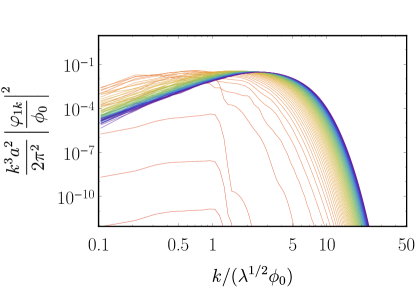
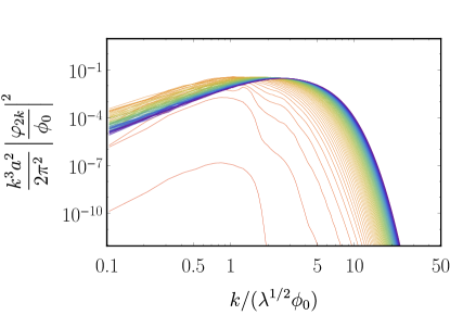
Figure 5: Same as Fig. 4, but for the real (left panel) and imaginary (right panel) components of the complex field $\varphi$. The growth of a broad range of comoving modes depicted by the light red curves is delayed with respect to the growth in the gauge field power spectrum from Fig. 4. It begins only around the time of backreaction of the gauge field on the $\varphi$ condensate. The reason why there is no resonant instability in the real components of $\varphi$ (and only in the gauge field) is our choice of parameters, $e^{2}=\lambda$. For more details see the main text and Ref. [113]. Following backreaction, the power in both components settles to a constant distribution.

Field Power Spectra: In Fig. 4, we plot the evolution of the gauge field power spectrum. Soon after the simulations commence, there is a rapid excitation of a broad range of $\delta\boldsymbol{\rm A}$ comoving wavenumbers, as depicted by the dark red curves in the figure. The power spectrum eventually stops growing, when backreaction kicks in. Later on, non-linear effects such as rescattering excite even a wider range of comoving modes and drive the gauge field power spectrum into a long-lived single-broad-peak configuration.

Unlike the gauge field power spectrum, the power spectra of the two scalar field components, shown in Fig. 5, do not feature the early rapid growth, as expected for our parameter choice, Eq. (4.3). A broad range of comoving $\varphi$ modes starts getting excited only around the time of backreaction of $\delta\boldsymbol{\rm A}$ on $\bar{\varphi}_{1}$, as depicted by the light red and orange curves in Fig. 5. At late times, mode-mode couplings again drive the $\varphi$ power spectra into a long-lived broad single-peaked configuration.

Energy fraction and equation of state evolution: The two-stage evolution (an initial $\bar{\varphi}_{1}$ oscillatory stage with $\delta\boldsymbol{\rm A}$ growing, followed by a long-lived steady-state nonlinear stage) can be also observed in the evolution of the fractional energies

$$f_{i} \equiv\frac{E_{i}}{E_{\rm tot}}\,,\qquad E_{i}=\int d^{3}\boldsymbol{\rm x}\,\rho_{i}(\boldsymbol{\rm x})\,,\qquad E_{\rm tot}=\sum_{i}E_{i}\,,$$ (4.4)

$$\rho_{K} =\frac{\varphi_{1}^{\prime 2}}{2a^{2}}+\frac{\varphi_{2}^{\prime 2}}{2a^{2}}\,,\qquad\rho_{V}=V\,,\qquad\rho_{\rm grad}=\frac{|\mathcal{D}_{i}\varphi|^{2}}{a^{2}}\,,$$

$$\rho_{\rm elec} =\frac{F_{0j}F_{0j}}{2e^{2}a^{4}}\,,\qquad\rho_{\rm magn}=\frac{F_{ij}F_{ij}}{4e^{2}a^{4}}\,,$$

given in the left panel in Fig. 6. For $\tau$ between $0$ and $\sim 70(\sqrt{\lambda}\phi_{0})^{-1}$, most of the total energy, $E_{\rm tot}$ is stored in the oscillating $\bar{\varphi}_{1}$, in the form of kinetic and potential energy. Afterwards, as non-linear effects become important the energy gets quickly redistributed across all components. At around $\tau\sim 200(\sqrt{\lambda}\phi_{0})^{-1}$, the system enters the long-lived non-linear stage, characterized by a steady energy equipartition [96]. Thereafter, the $\varphi$ self-interaction potential energy vanishes, $f_{\rm pot}\approx 0$, whereas $f_{\rm kin}\approx f_{\rm grad}$ and $f_{\rm elec}\approx f_{\rm magn}$.

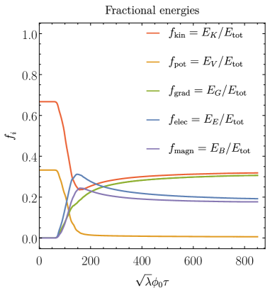
Figure 6: The evolution of the normalized energies (left panel), see Eq. (4.4), and the equation of state (right panel), see Eq. (4.5), for the case of $v=0$. All quantities are rapidly oscillating, so the curves are the smoothed time-averages over several oscillations. In the left panel we clearly see the initial oscillatory phase, during which all of the energy is stored in the oscillating $\bar{\varphi}_{1}$ background in the form of kinetic and potential energy. After backreaction by the gauge fields aournd $\tau\sim 70(\sqrt{\lambda}\phi_{0})^{-1}$, energy quickly gets redistributed across all components and the curves approach horizontal asymptotics. At late times, both the Higgs and the gauge field behave as massless radiation, which is reflected by the equation of state on the right.

Our numerical algorithm also allowed us, for the first time, to compute the self-consistent expansion of the FRW background sourced by an inhomogeneous scalar electrodynamics system. The evolution of the mean equation of state, $w$,

$$w=\frac{p}{\rho}=f_{K}-f_{V}+\frac{1}{3}(f_{\rm elec}+f_{\rm magn}-f_{\rm grad})\,,$$ (4.5)

is shown in the right panel in Fig. 6. We find that $w=1/3$ throughout, which is to be expected. During the initial oscillatory stage, we have a single homogeneous oscillating scalar field with a quartic self-interaction, which implies the well-known result of $1/3$ for the mean equation of state [115] (in our notation, the only non-zero $f_{i}$s are $f_{K}=2f_{V}=2/3$). Later on, since the $\varphi$ self-interaction potential energy vanishes, the real and imaginary parts of $\varphi$, as well as the components of the gauge fields behave as massless radiation, again implying a radiation-like equation of state (in our notation in the radiation limit, $f_{K}+f_{\rm elec}\approx 1/2$, since the magnetic and electromagnetic components are approximately equal, as well as the Higgs kinetic and gradient energies).

Lattice snapshots: Individual snapshots of the field configurations and their energy densities on the lattice at any given time reveal a rich spatial structure in the fields at both the linear and nonlinear stages. In Fig. 7, we provide an example of snapshots of the fractional electric and magnetic field densities at three different times. The initial resonance instability leads to a growth of large length-scale modes with a somewhat larger fraction in electric fields. The third panel reveals a more scrambled configuration at late times (after backreaction). While we do not do so here, plotting the vector field configurations (rather than scalar energy densities), or pseudoscalar quantities such as $({\bf E}\cdot{\bf B})$ also provides useful insight into the complex underlying dynamics.

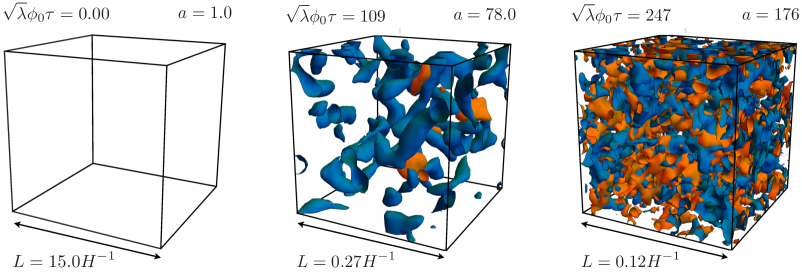
Figure 7: The evolution of the normalized electric (blue) and magnetic (orange) field energy densities for the case where $v=0$ (no symmetry breaking). The contours are drawn at $f_{i}=\rho_{i}/\rho_{\rm tot}=0.4$ where $i=E,B$. The middle panel is close to the time when backreaction begins. The rightmost panel is at late times after the $\varphi$ condensate has fragmented. Note that this figure is produced from half the box compared to the rest of the text.

Energy and Gauss constraint preservation: To keep track of the violation of the energy conservation in our simulations, we consider the quantity

$$\mathcal{E}\equiv\frac{|\mathcal{C}_{\mathcal{E}}|}{a^{2}\rho}=\left|1-\frac{3m_{\mbox{\tiny{Pl}}}^{2}\mathcal{H}^{2}}{a^{2}\rho}\right|\,.$$ (4.6)

where $\mathcal{C}_{\mathcal{E}}$ was defined in section Eq. (2.11). For the simulation whose results we have been discussing so far, the evolution of $\mathcal{E}$ is shown in the left panel in Fig. 8. Note that it is easy to achieve a very small degree of energy violation, $<10^{-5}$, with a fairly large time step, due to the high order of the symplectic time integrator. Furthermore, the energy violation is quite stable and grows very slowly, due to the time-reversability of symplectic integrators.

We characterize the violation of the Gauss constraint with the quantity (see Eq. (2.26))

$$\mathcal{G}(\boldsymbol{\rm x})=\frac{e^{-2}|\mathcal{C}_{\rm G}(\tau,\textbf{x})|}{\sqrt{(\boldsymbol{\nabla}\cdot\boldsymbol{\pi}_{\!A}(\tau,\textbf{x}))^{2}+\left[\pi_{1}(\tau,\textbf{x})\varphi_{2}(\tau,\textbf{x})-\pi_{2}(\tau,\textbf{x})\varphi_{1}(\tau,\textbf{x})\right]^{2}}}\,.$$ (4.7)

We show its evolution at an arbitrary lattice point, $\boldsymbol{\rm x}$, in the right panel in Fig. 8. The algorithm performance is excellent, with the violation never exceeding $10^{-6}$ and for most of the time remaining close to machine precision. The brief increase in the violation is observed only during the oscillatory phase, while the $\varphi$ field is still homogeneous. During this period, the calculation of spatial derivatives and/or differences of products of fields might lead to numerical errors due to attempting to compute small differences between large numbers, a phenomenon known as differencing noise. The observed growth in the violation during the oscillatory stage could be explained by such numerical errors.

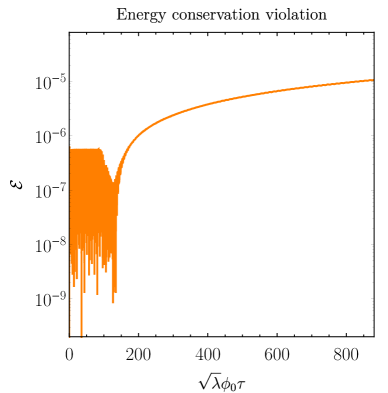
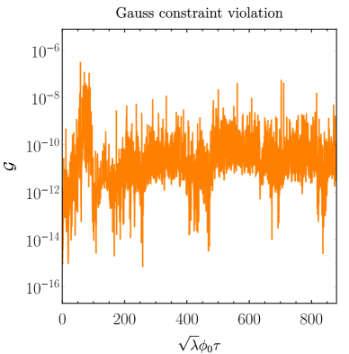
Figure 8: The evolution of the violations of energy conservation (left panel), see Eq. (4.6), and the Gauss constraint (right panel), see Eq. (4.7) for the case where $v=0$. The energy violation is very stable which is a generic property of symplectic integrators. The Gauss constraint violation starts growing from being close to machine precision initially due to finite differencing noise during the initial homogeneous oscillatory stage. As the Higgs fragments, the violation settles down to a constant small value. Note that we have defined $\mathcal{E}$ and $\mathcal{G}$ to be positive definite.

4.2 Nonlinear dynamics in the $v\neq 0$ case

We move on to the $v\neq 0$ case, for which the profile of the Higgs potential, $V(\varphi)$, resembles a sombrero hat, see right panel in Fig. 3. We set

$$v=1.32\times 10^{-2}m_{\mbox{\tiny{Pl}}}\,,$$ (4.8)

which is in agreement with Eq. (4.2). For the coupling constant $e$, we again use the value from Eq. (4.3).

Field Power Spectra: The initial evolution of the system proceeds in the same manner as in the previous case from Section 4.1. Since the $v$ from Eq. (4.8) is much less than the typical amplitude of $\bar{\varphi}_{1}$ oscillations, see Eq. (4.2), the initial parametric resonance phase is unaffected by $v$. We still have significant $\delta\boldsymbol{\rm A}$ resonant particle production. Again parametric resonance does not develop in the Higgs due to our choice of $e$, as explained in Section 4.1. Only once $\delta\boldsymbol{\rm A}$ begins to backreact, there is significant amplification of a broad range of comoving Higgs modes. After backreaction, the power spectra of the Higgs and the gauge fields again settle into stable broad single-peaked configurations. Since the power spectra plot are qualitatively similar to the $v=0$ case, we have relegated them to an appendix.

Cosmic strings: Plotting the evolution of the fields in real space, reveals a phenomenon that cannot be picked out from the evolution of the power spectra. Note that the $v\neq 0$ Higgs potential (right panel in Fig. 3), can support the non-trivial field configurations known as topological strings [116]. They can be generated during thermal phase transitions via the Kibble mechanism in the form of cosmic string networks (for reviews see, e.g., [117, 14, 15, 118]). Strings can be also produced after backreaction due to parametric resonance [119, 120, 121, 27], just like in our case. Since strings are characterized by a non-zero integer topological number, known as the winding number, $n$,

$$n\equiv\frac{1}{2\pi}\oint d{\boldsymbol{l}}\cdot{\boldsymbol{\nabla}}\arg(\varphi)\,,$$ (4.9)

we plot the lattice points with $n\neq 0$ at four different times in Fig. 9.

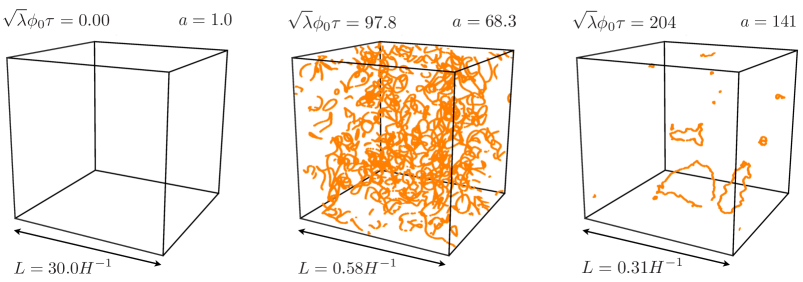
Figure 9: Snapshots of the simulation box at four different times for the case where $V(\varphi)$ has a Sombrero-hat shape. The orange points have non-zero winding number, $n$, see Eq. (4.9). The physical size of the simulation box, $L$, is given in units of the Hubble radius, $H^{-1}$. There is a copious production of subhorizon Nielsen-Olesen string loops around the time of backreaction. The loops eventually start to evaporate away. In the last panel the string core is resolved by $\mathcal{O}[10]$ points per linear dimension.

The first panel in Fig. 9 is at the start of the simulation. All lattice points have $n=0$, consistent with the inflationary initial conditions, see Eqs. (LABEL:eq:InitBckgrnd) and (3.16). Towards the end of the resonant particle production and the onset of backreaction we observe copious formation of strings and string loops with a sub-Hubble correlation length, as shown in the second panel in Fig. 9. The strings then interact, reconnect into loops and gradually evaporate via classical radiation. We see features developing on loops, which split from the larger loop to form smaller loops, which then decay away. The last large loop in our simulation is seen (third panel in Fig. 9) around the time the fields enter the long-lived steady-state non-linear stage. At this stage, the string core is resolved by roughly 10 points per linear dimension. A more dedicated recent study of decay of single loops can be found in [122]. At late times, there are no strings in our box, which is consistent with the conservation of the net winding number and our initial conditions having zero $n$. We note that the string configurations never dominate the energy density in our box.

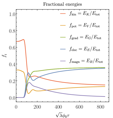
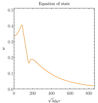
Figure 10: Same as Fig. 6, but for $v\neq 0$. The initial oscillatory phase of homogeneous $\bar{\varphi}_{1}$ is still clearly visible in both panels. However, after backreaction, the complex Higgs falls into the potential valley at $|\varphi|=v/\sqrt{2}$, see Fig. 3. All dynamical components are now massive. The radial component of the Higgs (stuck near the bottom of potential valley) behaves as a massive scalar, as reflected by the red and orange curves in the left panel. The azimuthal component of the Higgs gets ‘eaten up’ by the gauge field, rendering the latter massive, as depicted by the blue and green curves in the left panel. Note that $f_{\rm grad}$ includes the gauge field mass term from the Higgs mechanism. The magnetic energy gets diluted away, since it redshifts faster than the kinetic and potential energies of the massive Higgs and gauge fields, as shown by the purple curve in the left panel. The evolution of the equation of state (right panel) captures this transition from a radiation-like to a matter-like state of expansion.

Energy fraction and equation of state evolution: The evolution of the mean fractional energies, $f_{i}$, is shown in the left panel in Fig. 10. Just like in the case with zero $v$ from Section 4.1, we again have two distinct regimes with a brief transitionary period inbetween. During the initial oscillatory phase, most of the energy is stored in the oscillating $\bar{\varphi}_{1}$, again with $f_{\rm kin}\approx 2f_{\rm pot}$. This approximate equality (which is exact for a quartic Higgs potential) becomes less accurate with time, since the amplitude of $\bar{\varphi}_{1}\propto a^{-1}$ and the $v^{2}$ term in $V$ becomes increasingly important. Backreaction occurs around $\tau\sim 80(\sqrt{\lambda}\phi_{0})^{-1}$ and is followed by a swift redistribution of energy. By $\tau\sim 200(\sqrt{\lambda}\phi_{0})^{-1}$, the last string loops start evaporating and the fields settle on a long and steady approach to equipartition.

After this point, at almost every location on the lattice, the $\varphi$ field has settled into the valley $V(|\varphi|=v/\sqrt{2}$). The radial component of the $\varphi$ field oscillates above the vev with amplitude $\ll v$ in a spatially inhomogeneous manner. Note that the radial Higgs component behaves as a massive scalar, since the bottom of the valley at $|\varphi|=v/\sqrt{2}$ is quadratic. The azimuthal Higgs component (the massless Nambu-Goldstone boson) is ‘eaten up’ by the gauge field like in the conventional Higgs mechanism, rendering the gauge field a massive vector field. Hence, both the radial Higgs degree of freedom and the gauge field behave as massive fields. They have massive non-relativistic modes, whose energy density redshifts as $\propto a^{-3}$, slower than the energy density of the relativistic modes (which scales as $\propto a^{-4}$). This implies that after a few e-folds of expansion, both the radial Higgs component and the gauge field should behave as pressureless matter, with potential and kinetic energies equal to each other and much greater than the gradient and curl energies. In our notation, this means that for the radial component of the Higgs, $f_{\rm kin}\rightarrow f_{\rm pot}$, whereas for the gauge field $f_{\rm elec}\rightarrow f_{\rm grad}$ (recall that the ‘potential’ mass term for the gauge field is contained in $f_{\rm grad}$, see Eq. (4.4)) and $f_{\rm magn}\rightarrow 0$. Indeed, this is the late-time behaviour shown in the left panel in Fig. 10.

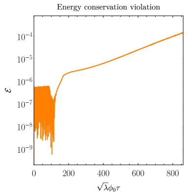
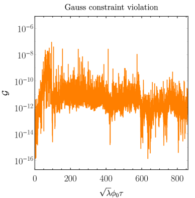
Figure 11: Same as Fig. 8, but for $v\neq 0$. The evolution of the violations of the energy conservation and Gauss constraint are qualitatively similar to the $v=0$ case. The slight difference is a small increase at late times of the energy violation only. It is due to the fact that we integrate in conformal time, whereas at late times the system is dominated by heavy, non-relativistic modes, see Fig. 10. For a possible improvement, see Fig. 12.

The self-consistent evolution of the mean equation of state, $w$ (see Eq. (4.5) for its definition) is given for the first time in the right panel in Fig. 10. Initially, it has a radiation-like value, due to the oscillations of the background $\bar{\varphi}_{1}$. The growing deviation from $1/3$ is due to the $v^{2}$ in $V$ becoming increasingly important as the amplitude of the oscillating $\bar{\varphi}_{1}$ is redshifted. After backreaction, $w$ steadily approaches $0$, since both the gauge field and the radial component of the complex Higgs field are massive. Their relativistic pressures are redshifted away, leaving behind pressureless scalar and vector dust with $w\rightarrow 0$.

Energy and Gauss Constraint: The energy conservation is shown in the left panel in Fig. 11. We have used the same lattice parameters as for the simulation from Section 4.1. The energy conservation is still excellent, $\leq 10^{-4}$. It is almost identical to the one for the $v=0$ case given in the left panel in Fig. 8, worsening only slightly at late times. The reason for this slightly worse performance for $v\neq 0$ can be traced back to the fact that we work with a fixed conformal-time step, $\Delta\tau$. For $v=0$, i.e., a quartic Higgs potential, the typical frequency scales always decrease with time as $\propto a^{-1}$, implying that their product with the cosmic-time step, $a(\tau)\Delta\tau$, is constant.

On the other hand, for the massive case, $v\neq 0$, the typical frequency scales are constant, implying that their product with the cosmic-time step grows like $\propto a(\tau)$, thereby increasing the time-integration error. Even though it was not necessary for this study, this small degradation in energy conservation can be easily alleviated by decreasing the conformal-time step only slightly. This takes advantage of the fact that the order of the time integrator, $k$, is high and the energy conservation is quite sensitive to the time step. The local truncation error in the time integration is $\mathcal{O}(\Delta\tau^{k+1})$, see Eq. (3.6), and the total accumulated error is $\mathcal{O}(\Delta\tau^{k})$. For $k=4$, the energy conservation can be improved by one or two orders of magnitude, when we decrease the conformal-time step only by a factor of $10^{1/4}$ or $10^{1/2}$, respectively, as shown in Fig. 12.

The Gauss constraint violation is shown in the right panel in Fig. 11 for a random lattice point. We find that it is qualitatively identical to the one for the $v=0$ case given in Fig. 8. It is also insensitive to the conformal-time step, which is expected for a quantity dominated by differencing noise.

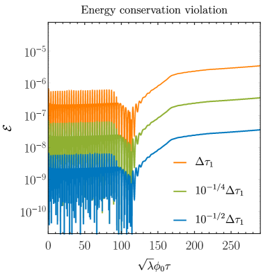
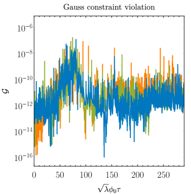
Figure 12: Left panel:The energy conservation for three different conformal time steps. The red curve is for the case from the left panel in Fig. 11. The green and blue curves are for the same simulation and model parameters, but for time steps $10^{1/4}$ and $10^{1/2}$ times smaller. The used symplectic integrator was of fourth order, $k=4$, and the energy conservation scales appropriately with the time step, $\propto\mathcal{O}(\Delta\tau^{k})$. Right panel: As expected from our algorithm, the violation of the Gauss constraint does not depend on the size of the time step.

5 Discussion

We have presented a novel prescription for numerically evolving Scalar Electrodynamics in FRW spacetime (sometimes also referred to Abelian-Higgs system, or explicitly, a charged scalar minimally coupled to Abelian gauge fields) . Our prescription combines two different well-known techniques in numerical simulations of related systems, one for handling the spatial derivatives, and another for temporal derivatives. The spatial discretization is carried out according to the Lattice Gauge Field theory prescription (using the lattice links formalism). The time evolution is performed with symplectic integrators. The algorithm allows for the self-consistent evolution of the FRW scale factor and fields, while respecting the Gauss constraint exactly on the discretized lattice. To the best of our knowledge, this is the first explicit-in-time algorithm which guarantees the preservation of of the Gauss constraint, while solving for the expansion of the universe self-consistently. In addition, the time integrator can be made of arbitrary high order, without violating any of the algorithm’s properties.

The use of symplectic integrators was inspired by already existing scalar field lattice codes such as HLattice [72], Defrost [71] and PyCool [73]. They are known for their excellent energy conservation and stability, when solving for the expansion of the universe self-consistently. Perhaps, one of the reasons why such integrators have not been employed in gauge field studies is the uncertainty of whether they will respect the Gauss constraint equation – a non-dynamical equation which always appears in gauge field theories, but never in pure-scalar models.

The issue with the Gauss constraint equation has long been solved in flat spacetime, by discretizing the Higgs field on a 4d rigid lattice, and defining the gauge fields on the lattice links. This method has been successfully extended to FRW spacetimes, with the scale factor evolving according to some fixed power-law, e.g., $a(\tau)\propto\tau$, not determined by the evolution of the Higgs and gauge fields [27, 96].

Given these successes, we employed a combination of the two approaches to achieve both good self-consistent expansion and preservation of the Gauss constraint. We showed how to combine them in a very straightforward way. To use symplectic integrators, we needed a simple Hamiltonian. The Hamiltonian for Scalar Electrodynamics was simplified substantially by working in the $A_{0}=0$ gauge. This gauge choice made all kinetic terms canonical, which in turn gave use a symplectic integrator for the time evolution. The remaining spatial derivatives were discretized by defining the complex scalar and the 3-components of the gauge field on a 3d spatial lattice, similarly to Lattice Gauge Field theory (with the use of Link variables). This automatically allowed the system to respect the residual gauge freedom in $A_{0}=0$ gauge. More importantly, this spatial discretization yielded a well-defined expression for the lattice version of the Gauss constraint, consistent with the residual symmetries. This version of the Gauss constraint turned out to be respected exactly by the symplectic integrators.

Numerical Studies: To test our algorithm and code, we investigated two different reheating scenarios. In both, the role of the oscillating inflaton was played by the real component of the complex scalar field. In the first scenario, the scalar potential was a simple quartic minimum (i.e., ‘unbroken’), whereas in the second one, the scalar field potential allowed for spontaneous symmetry breaking (a Higgs-like potential). The lattice simulations captured the initial preheating phase in which the gauge field was excited non-perturbatively due to parametric resonance in the oscillating homogeneous scalar field background. They also revealed the subsequent non-linear stage after backreaction and fragmentation of the condensate. All qualitative predictions of linear analyses for the resonant particle production were reproduced. The subsequent non-linear stage included interesting non-linear phenomena such as the formation and disappearance of Nielsen-Olesen strings (in the case with the symmetry breaking potential).

The self-consistent FRW expansion was computed throughout – the energy conservation violation was stable, being always $\leq 10^{-4}$ and scaling appropriately with the size of the time step, $\propto\Delta\tau^{k}$ for a $k$th-order integrator. As expected, the case with unbroken scalar field potential lead to a radiation-like equation of state during the oscillatory as well as the non-linear stages. Similarly, a late-time matter-like state of expansion predicted for the spontaneously broken case (since along with the radial part of the scalar, the gauge fields are now massive), was reproduced during the non-linear stage. In both cases the Gauss constraint was preserved, with violations $<10^{-6}$; these violations were dominated by numerical errors due to subtraction of large quantities with very small differences (differencing noise).

Limitations: We note that the combination of a symplectic time integrator and a Lattice Gauge Field type of discretization does not seem to work for non-Abelian gauge theories, e.g., an $SU(2)$ Yang-Mills theory with a Higgs doublet. In this case, the Gauss constraint is not respected by the symplectic integrator. A reason for that could be the non-linear nature of the Gauss constraint in non-Abelian theories. Another class of gauge field models which is not well-suited for our prescription is the one featuring an axion, $\chi$. Both Abelian and non-Abelian theories with a Chern-Simons type of interaction, $\propto\chi F\tilde{F}$, cannot be integrated symplectically due to the non-canonical structure of the gauge field kinetic term. However, an interaction of the form $\propto\chi F^{2}$ could work at least in Abelian theories, since the kinetic term of the gauge field is canonical up to an axion-dependent rescaling, meeting the conditions for usage of symplectic integrators.

We hope that ${\sf GFiRe}$ will be used for many more cosmological studies of non-linear gauge field dynamics. We plan to make ${\sf GFiRe}$ public in the near future.

Appendix A Power Spectra for $v\neq 0$ case

We provide the time evolution of the power spectra for the gauge fields as well as the real and imaginary components of the $\varphi$ field below in the $v\neq 0$ case. See corresponding discussion in the main text.

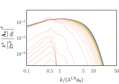
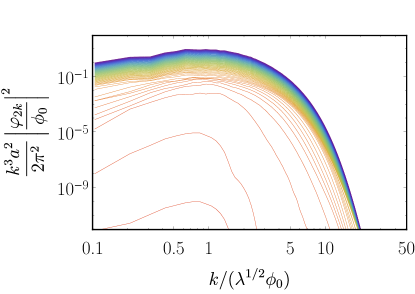
Figure 13: The evolution of the power spectra is qualitatively the same as in the $v=0$ case.

References

- [1] A. D. Dolgov and D. P. Kirilova, ON PARTICLE CREATION BY A TIME DEPENDENT SCALAR FIELD, Sov. J. Nucl. Phys. 51 (1990) 172.
- [2] J. H. Traschen and R. H. Brandenberger, Particle Production During Out-of-equilibrium Phase Transitions, Phys. Rev. D42 (1990) 2491.
- [3] L. Kofman, A. D. Linde and A. A. Starobinsky, Reheating after inflation, Phys. Rev. Lett. 73 (1994) 3195 [hep-th/9405187].
- [4] Y. Shtanov, J. H. Traschen and R. H. Brandenberger, Universe reheating after inflation, Phys. Rev. D51 (1995) 5438 [hep-ph/9407247].
- [5] L. Kofman, A. D. Linde and A. A. Starobinsky, Towards the theory of reheating after inflation, Phys. Rev. D56 (1997) 3258 [hep-ph/9704452].
- [6] B. A. Bassett, S. Tsujikawa and D. Wands, Inflation dynamics and reheating, Rev. Mod. Phys. 78 (2006) 537 [astro-ph/0507632].
- [7] R. Allahverdi, R. Brandenberger, F.-Y. Cyr-Racine and A. Mazumdar, Reheating in Inflationary Cosmology: Theory and Applications, Ann. Rev. Nucl. Part. Sci. 60 (2010) 27 [1001.2600].
- [8] A. V. Frolov, Non-linear Dynamics and Primordial Curvature Perturbations from Preheating, Class. Quant. Grav. 27 (2010) 124006 [1004.3559].
- [9] M. A. Amin, M. P. Hertzberg, D. I. Kaiser and J. Karouby, Nonperturbative Dynamics Of Reheating After Inflation: A Review, Int. J. Mod. Phys. D24 (2014) 1530003 [1410.3808].
- [10] K. D. Lozanov, Lectures on Reheating after Inflation, 1907.04402.
- [11] D. I. Podolsky, G. N. Felder, L. Kofman and M. Peloso, Equation of state and beginning of thermalization after preheating, Phys. Rev. D73 (2006) 023501 [hep-ph/0507096].
- [12] K. D. Lozanov and M. A. Amin, Equation of State and Duration to Radiation Domination after Inflation, Phys. Rev. Lett. 119 (2017) 061301 [1608.01213].
- [13] K. D. Lozanov and M. A. Amin, Self-resonance after inflation: oscillons, transients and radiation domination, Phys. Rev. D97 (2018) 023533 [1710.06851].
- [14] M. B. Hindmarsh and T. W. B. Kibble, Cosmic strings, Rept. Prog. Phys. 58 (1995) 477 [hep-ph/9411342].
- [15] E. J. Copeland and T. W. B. Kibble, Cosmic Strings and Superstrings, Proc. Roy. Soc. Lond. A466 (2010) 623 [0911.1345].
- [16] M. A. Amin, R. Easther, H. Finkel, R. Flauger and M. P. Hertzberg, Oscillons After Inflation, Phys. Rev. Lett. 108 (2012) 241302 [1106.3335].
- [17] M. Gleiser, N. Graham and N. Stamatopoulos, Generation of Coherent Structures After Cosmic Inflation, Phys. Rev. D83 (2011) 096010 [1103.1911].
- [18] K. Enqvist, S. Kasuya and A. Mazumdar, Inflatonic solitons in running mass inflation, Phys. Rev. D 66 (2002) 043505.
- [19] M. A. Amin and P. Mocz, Formation, gravitational clustering, and interactions of nonrelativistic solitons in an expanding universe, Phys. Rev. D100 (2019) 063507 [1902.07261].
- [20] J. C. Niemeyer and R. Easther, Inflaton Clusters and Inflaton Stars, 1911.01661.
- [21] N. Musoke, S. Hotchkiss and R. Easther, Lighting the Dark: The Evolution of the Post-Inflationary Universe, 1909.11678.
- [22] A. Chambers and A. Rajantie, Lattice calculation of non-Gaussianity from preheating, Phys. Rev. Lett. 100 (2008) 041302 [0710.4133].
- [23] J. R. Bond, A. V. Frolov, Z. Huang and L. Kofman, Non-Gaussian Spikes from Chaotic Billiards in Inflation Preheating, Phys. Rev. Lett. 103 (2009) 071301 [0903.3407].
- [24] S. V. Imrith, D. J. Mulryne and A. Rajantie, Primordial curvature perturbation from lattice simulations, Phys. Rev. D100 (2019) 043543 [1903.07487].
- [25] S. Y. Khlebnikov and I. I. Tkachev, Relic gravitational waves produced after preheating, Phys. Rev. D56 (1997) 653 [hep-ph/9701423].
- [26] R. Easther and E. A. Lim, Stochastic gravitational wave production after inflation, JCAP 0604 (2006) 010 [astro-ph/0601617].
- [27] J.-F. Dufaux, D. G. Figueroa and J. Garcia-Bellido, Gravitational Waves from Abelian Gauge Fields and Cosmic Strings at Preheating, Phys. Rev. D82 (2010) 083518 [1006.0217].
- [28] K. D. Lozanov and M. A. Amin, Gravitational perturbations from oscillons and transients after inflation, 1902.06736.
- [29] P. Adshead, J. T. Giblin, M. Pieroni and Z. J. Weiner, Constraining axion inflation with gravitational waves from preheating, 1909.12842.
- [30] P. Adshead, J. T. Giblin, M. Pieroni and Z. J. Weiner, Constraining axion inflation with gravitational waves across 29 decades in frequency, 1909.12843.
- [31] S.-Y. Zhou, E. J. Copeland, R. Easther, H. Finkel, Z.-G. Mou and P. M. Saffin, Gravitational Waves from Oscillon Preheating, JHEP 10 (2013) 026 [1304.6094].
- [32] S. Antusch, F. Cefala and S. Orani, Gravitational waves from oscillons after inflation, Phys. Rev. Lett. 118 (2017) 011303 [1607.01314].
- [33] S. Antusch, F. Cefala, S. Krippendorf, F. Muia, S. Orani and F. Quevedo, Oscillons from String Moduli, JHEP 01 (2018) 083 [1708.08922].
- [34] S. Antusch, F. Cefala and S. Orani, What can we learn from the stochastic gravitational wave background produced by oscillons?, JCAP 1803 (2018) 032 [1712.03231].
- [35] J. Liu, Z.-K. Guo, R.-G. Cai and G. Shiu, Gravitational wave production after inflation with cuspy potentials, Phys. Rev. D99 (2019) 103506 [1812.09235].
- [36] R. Easther, J. T. Giblin, Jr. and E. A. Lim, Gravitational Wave Production At The End Of Inflation, Phys. Rev. Lett. 99 (2007) 221301 [astro-ph/0612294].
- [37] J. Garcia-Bellido, D. G. Figueroa and A. Sastre, A Gravitational Wave Background from Reheating after Hybrid Inflation, Phys. Rev. D77 (2008) 043517 [0707.0839].
- [38] J. F. Dufaux, A. Bergman, G. N. Felder, L. Kofman and J.-P. Uzan, Theory and Numerics of Gravitational Waves from Preheating after Inflation, Phys. Rev. D76 (2007) 123517 [0707.0875].
- [39] J.-F. Dufaux, G. Felder, L. Kofman and O. Navros, Gravity Waves from Tachyonic Preheating after Hybrid Inflation, JCAP 0903 (2009) 001 [0812.2917].
- [40] N. Bartolo et al., Science with the space-based interferometer LISA. IV: Probing inflation with gravitational waves, JCAP 1612 (2016) 026 [1610.06481].
- [41] D. G. Figueroa and F. Torrenti, Gravitational wave production from preheating: parameter dependence, JCAP 1710 (2017) 057 [1707.04533].
- [42] C. Caprini and D. G. Figueroa, Cosmological Backgrounds of Gravitational Waves, Class. Quant. Grav. 35 (2018) 163001 [1801.04268].
- [43] N. Bartolo, V. Domcke, D. G. Figueroa, J. García-Bellido, M. Peloso, M. Pieroni et al., Probing non-Gaussian Stochastic Gravitational Wave Backgrounds with LISA, JCAP 1811 (2018) 034 [1806.02819].
- [44] C. Armendariz-Picon, On the Expected Production of Gravitational Waves During Preheating, JCAP 1908 (2019) 012 [1905.05724].
- [45] M. I. Khlopov, B. A. Malomed and I. B. Zeldovich, Gravitational instability of scalar fields and formation of primordial black holes, Mon. Not. R. Astron. Soc. 215 (1985) 575.
- [46] E. Cotner, A. Kusenko, M. Sasaki and V. Takhistov, Analytic Description of Primordial Black Hole Formation from Scalar Field Fragmentation, 1907.10613.
- [47] J. Martin, T. Papanikolaou and V. Vennin, Primordial black holes from the preheating instability, 1907.04236.
- [48] J. Garcia-Bellido, A. D. Linde and D. Wands, Density perturbations and black hole formation in hybrid inflation, Phys. Rev. D54 (1996) 6040 [astro-ph/9605094].
- [49] A. M. Green and K. A. Malik, Primordial black hole production due to preheating, Phys. Rev. D64 (2001) 021301 [hep-ph/0008113].
- [50] J. C. Hidalgo, L. A. Urena-Lopez and A. R. Liddle, Unification models with reheating via Primordial Black Holes, Phys. Rev. D85 (2012) 044055 [1107.5669].
- [51] E. Torres-Lomas, J. C. Hidalgo, K. A. Malik and L. A. Ureña-López, Formation of subhorizon black holes from preheating, Phys. Rev. D89 (2014) 083008 [1401.6960].
- [52] T. Suyama, T. Tanaka, B. Bassett and H. Kudoh, Are black holes over-produced during preheating?, Phys. Rev. D71 (2005) 063507 [hep-ph/0410247].
- [53] T. Suyama, T. Tanaka, B. Bassett and H. Kudoh, Black hole production in tachyonic preheating, JCAP 0604 (2006) 001 [hep-ph/0601108].
- [54] E. Cotner, A. Kusenko and V. Takhistov, Primordial Black Holes from Inflaton Fragmentation into Oscillons, Phys. Rev. D98 (2018) 083513 [1801.03321].
- [55] M. A. G. Garcia and M. A. Amin, Prethermalization production of dark matter, Phys. Rev. D98 (2018) 103504 [1806.01865].
- [56] K. D. Lozanov and M. A. Amin, End of inflation, oscillons, and matter-antimatter asymmetry, Phys. Rev. D90 (2014) 083528 [1408.1811].
- [57] M. P. Hertzberg and J. Karouby, Baryogenesis from the Inflaton Field, Phys. Lett. B737 (2014) 34 [1309.0007].
- [58] K. Enqvist and J. McDonald, Q balls and baryogenesis in the MSSM, Phys. Lett. B425 (1998) 309 [hep-ph/9711514].
- [59] M. Hindmarsh and A. Rajantie, Phase transition dynamics in the hot Abelian Higgs model, Phys. Rev. D64 (2001) 065016 [hep-ph/0103311].
- [60] J. T. Giblin, G. Kane, E. Nesbit, S. Watson and Y. Zhao, Was the Universe Actually Radiation Dominated Prior to Nucleosynthesis?, Phys. Rev. D96 (2017) 043525 [1706.08536].
- [61] M. A. Amin, J. Fan, K. D. Lozanov and M. Reece, Cosmological dynamics of Higgs potential fine tuning, Phys. Rev. D99 (2019) 035008 [1802.00444].
- [62] E. W. Kolb and I. I. Tkachev, Nonlinear axion dynamics and formation of cosmological pseudosolitons, Phys. Rev. D49 (1994) 5040 [astro-ph/9311037].
- [63] N. Kitajima, J. Soda and Y. Urakawa, Gravitational wave forest from string axiverse, JCAP 1810 (2018) 008 [1807.07037].
- [64] M. Buschmann, J. W. Foster and B. R. Safdi, Early-Universe Simulations of the Cosmological Axion, 1906.00967.
- [65] H. Fukunaga, N. Kitajima and Y. Urakawa, Efficient self-resonance instability from axions, JCAP 1906 (2019) 055 [1903.02119].
- [66] T. Patel, H. Tashiro and Y. Urakawa, Resonant magnetogenesis from axions, 1909.00288.
- [67] T. L. Smith, V. Poulin and M. A. Amin, Oscillating scalar fields and the Hubble tension: a resolution with novel signatures, 1908.06995.
- [68] S. Yu. Khlebnikov and I. I. Tkachev, Classical decay of inflaton, Phys. Rev. Lett. 77 (1996) 219 [hep-ph/9603378].
- [69] T. Prokopec and T. G. Roos, Lattice study of classical inflaton decay, Phys. Rev. D55 (1997) 3768 [hep-ph/9610400].
- [70] G. N. Felder and I. Tkachev, LATTICEEASY: A Program for lattice simulations of scalar fields in an expanding universe, Comput. Phys. Commun. 178 (2008) 929 [hep-ph/0011159].
- [71] A. V. Frolov, DEFROST: A New Code for Simulating Preheating after Inflation, JCAP 0811 (2008) 009 [0809.4904].
- [72] Z. Huang, The Art of Lattice and Gravity Waves from Preheating, Phys. Rev. D83 (2011) 123509 [1102.0227].
- [73] J. Sainio, PyCOOL - a Cosmological Object-Oriented Lattice code written in Python, JCAP 1204 (2012) 038 [1201.5029].
- [74] H. L. Child, J. T. Giblin, Jr, R. H. Ribeiro and D. Seery, Preheating with Non-Minimal Kinetic Terms, Phys. Rev. Lett. 111 (2013) 051301 [1305.0561].
- [75] R. Easther, H. Finkel and N. Roth, PSpectRe: A Pseudo-Spectral Code for (P)reheating, JCAP 1010 (2010) 025 [1005.1921].
- [76] M. A. Amin, J. Braden, E. J. Copeland, J. T. Giblin, C. Solorio, Z. J. Weiner et al., Gravitational waves from asymmetric oscillon dynamics?, Phys. Rev. D98 (2018) 024040 [1803.08047].
- [77] J. T. Giblin and A. J. Tishue, Preheating in Full General Relativity, 1907.10601.
- [78] J. Rubio and E. S. Tomberg, Preheating in Palatini Higgs inflation, JCAP 1904 (2019) 021 [1902.10148].
- [79] R. Nguyen, J. van de Vis, E. I. Sfakianakis, J. T. Giblin and D. I. Kaiser, Nonlinear Dynamics of Preheating after Multifield Inflation with Nonminimal Couplings, 1905.12562.
- [80] J. A. Crespo and H. P. de Oliveira, Aspects of wave turbulence in preheating II: Rebirth of the nonminimal coupled models, 1905.13647.
- [81] J. A. Crespo and H. P. de Oliveira, Aspects of wave turbulence in preheating III: The case of the two-fields models, 1906.00802.
- [82] H.-Y. Schive, T. Chiueh and T. Broadhurst, Cosmic Structure as the Quantum Interference of a Coherent Dark Wave, Nature Phys. 10 (2014) 496 [1406.6586].
- [83] B. Schwabe, J. C. Niemeyer and J. F. Engels, Simulations of solitonic core mergers in ultralight axion dark matter cosmologies, Phys. Rev. D94 (2016) 043513 [1606.05151].
- [84] F. Edwards, E. Kendall, S. Hotchkiss and R. Easther, PyUltraLight: A Pseudo-Spectral Solver for Ultralight Dark Matter Dynamics, JCAP 1810 (2018) 027 [1807.04037].
- [85] P. Adshead, J. T. Giblin, T. R. Scully and E. I. Sfakianakis, Gauge-preheating and the end of axion inflation, JCAP 1512 (2015) 034 [1502.06506].
- [86] P. Adshead, J. T. Giblin, T. R. Scully and E. I. Sfakianakis, Magnetogenesis from axion inflation, JCAP 1610 (2016) 039 [1606.08474].
- [87] P. Adshead, J. T. Giblin and Z. J. Weiner, Gravitational waves from gauge preheating, Phys. Rev. D98 (2018) 043525 [1805.04550].
- [88] J. R. C. Cuissa and D. G. Figueroa, Lattice formulation of axion inflation. Application to preheating, JCAP 1906 (2019) 002 [1812.03132].
- [89] D. G. Figueroa and M. Shaposhnikov, Lattice implementation of Abelian gauge theories with Chern–Simons number and an axion field, Nucl. Phys. B926 (2018) 544 [1705.09629].
- [90] D. G. Figueroa, A. Florio and M. Shaposhnikov, Chiral charge dynamics in Abelian gauge theories at finite temperature, 1904.11892.
- [91] J. Braden, L. Kofman and N. Barnaby, Reheating the Universe After Multi-Field Inflation, JCAP 1007 (2010) 016 [1005.2196].
- [92] J. T. Deskins, J. T. Giblin and R. R. Caldwell, Gauge Field Preheating at the End of Inflation, Phys. Rev. D88 (2013) 063530 [1305.7226].
- [93] P. Adshead, J. T. Giblin and Z. J. Weiner, Non-Abelian gauge preheating, Phys. Rev. D96 (2017) 123512 [1708.02944].
- [94] J. Smit, P. Goddard and J. Yeomans, Introduction to Quantum Fields on a Lattice, Cambridge Lecture Notes in Physics. Cambridge University Press, 2002.
- [95] A. Rajantie and E. J. Copeland, Phase transitions from preheating in gauge theories, Phys. Rev. Lett. 85 (2000) 916 [hep-ph/0003025].
- [96] D. G. Figueroa, J. Garcia-Bellido and F. Torrenti, Decay of the standard model Higgs field after inflation, Phys. Rev. D92 (2015) 083511 [1504.04600].
- [97] D. G. Figueroa, J. Garcia-Bellido and F. Torrenti, Gravitational wave production from the decay of the standard model Higgs field after inflation, Phys. Rev. D93 (2016) 103521 [1602.03085].
- [98] D. G. Figueroa and C. T. Byrnes, The Standard Model Higgs as the origin of the hot Big Bang, Phys. Lett. B767 (2017) 272 [1604.03905].
- [99] J. Garcia-Bellido, M. Garcia-Perez and A. Gonzalez-Arroyo, Chern-Simons production during preheating in hybrid inflation models, Phys. Rev. D69 (2004) 023504 [hep-ph/0304285].
- [100] N. Graham, An Electroweak oscillon, Phys. Rev. Lett. 98 (2007) 101801 [hep-th/0610267].
- [101] A. Diaz-Gil, J. Garcia-Bellido, M. Garcia Perez and A. Gonzalez-Arroyo, Magnetic field production during preheating at the electroweak scale, Phys. Rev. Lett. 100 (2008) 241301 [0712.4263].
- [102] N. Graham, Numerical Simulation of an Electroweak Oscillon, Phys. Rev. D76 (2007) 085017 [0706.4125].
- [103] A. Diaz-Gil, J. Garcia-Bellido, M. Garcia Perez and A. Gonzalez-Arroyo, Primordial magnetic fields from preheating at the electroweak scale, JHEP 07 (2008) 043 [0805.4159].
- [104] K. Enqvist, S. Nurmi, S. Rusak and D. Weir, Lattice Calculation of the Decay of Primordial Higgs Condensate, JCAP 1602 (2016) 057 [1506.06895].
- [105] Z.-G. Mou, P. M. Saffin and A. Tranberg, Simulations of Cold Electroweak Baryogenesis: Hypercharge U(1) and the creation of helical magnetic fields, JHEP 06 (2017) 075 [1704.08888].
- [106] A. Tranberg, S. Tähtinen and D. J. Weir, Gravitational waves from non-Abelian gauge fields at a tachyonic transition, JCAP 1804 (2018) 012 [1706.02365].
- [107] H. Yoshida, Construction of higher order symplectic integrators, Phys. Lett. A150 (1990) 262.
- [108] T. Krajewski, K. Turzynski and M. Wieczorek, On preheating in -attractor models of inflation, Eur. Phys. J. C79 (2019) 654 [1801.01786].
- [109] E. J. Weinberg, Classical solutions in quantum field theory, Cambridge Monographs on Mathematical Physics. Cambridge University Press, 2012, 10.1017/CBO9781139017787.
- [110] A. D. Linde, The inflationary universe, Reports on Progress in Physics 47 (1984) 925.
- [111] A. D. Linde, Particle physics and inflationary cosmology, Contemp. Concepts Phys. 5 (1990) 1 [hep-th/0503203].
- [112] Planck collaboration, Y. Akrami et al., Planck 2018 results. X. Constraints on inflation, 1807.06211.
- [113] K. D. Lozanov and M. A. Amin, The charged inflaton and its gauge fields: preheating and initial conditions for reheating, JCAP 1606 (2016) 032 [1603.05663].
- [114] S. Y. Khlebnikov and I. I. Tkachev, Classical decay of the inflaton, Phys. Rev. Lett. 77 (1996) 219.
- [115] M. S. Turner, Coherent Scalar Field Oscillations in an Expanding Universe, Phys. Rev. D28 (1983) 1243.
- [116] H. B. Nielsen and P. Olesen, Vortex-line models for dual strings, Nuclear Physics B 61 (1973) 45.
- [117] A. Vilenkin and E. P. S. Shellard, Cosmic Strings and Other Topological Defects. Cambridge University Press, 2000.
- [118] A. Drew and E. P. S. Shellard, Radiation from Global Topological Strings using Adaptive Mesh Refinement: Methodology and Massless Modes, 1910.01718.
- [119] G. N. Felder, L. Kofman and A. D. Linde, Tachyonic instability and dynamics of spontaneous symmetry breaking, Phys. Rev. D64 (2001) 123517 [hep-th/0106179].
- [120] I. Tkachev, S. Khlebnikov, L. Kofman and A. D. Linde, Cosmic strings from preheating, Phys. Lett. B440 (1998) 262 [hep-ph/9805209].
- [121] S. Kasuya and M. Kawasaki, Can topological defects be formed during preheating?, Phys. Rev. D56 (1997) 7597 [hep-ph/9703354].
- [122] D. Matsunami, L. Pogosian, A. Saurabh and T. Vachaspati, Decay of Cosmic String Loops Due to Particle Radiation, Phys. Rev. Lett. 122 (2019) 201301 [1903.05102].