Standard-model prediction of $\epsilon_{K}$ with manifest CKM unitarity

Abstract

The parameter $\epsilon_{K}$ describes CP violation in the neutral kaon system and is one of the most sensitive probes of new physics. The large uncertainties related to the charm-quark contribution to $\epsilon_{K}$ have so far prevented a reliable standard-model prediction. We show that CKM unitarity enforces a unique form of the $|\Delta{\rm S}\!=\!2|$ weak effective Lagrangian in which the short-distance theory uncertainty of the imaginary part is dramatically reduced. The uncertainty related to the charm-quark contribution is now at the percent level. We present the updated standard-model prediction $\epsilon_{K}=2.16(6)(8)(15)\times 10^{-3}$, where the errors in brackets correspond to QCD short-distance and long-distance, and parametric uncertainties, respectively.

I Introduction

CP violation in the neutral kaon system, parameterized by $\epsilon_{K}$, is one of the most sensitive precision probes of new physics. For decades, the large perturbative uncertainties related to the charm-quark contributions have been an impediment to fully exploiting the potential of $\epsilon_{K}$. In this letter we demonstrate how to overcome this obstacle.

The parameter $\epsilon_{K}$ can be defined as Anikeev et al. (2001)

$$\epsilon_{K}\equiv e^{i\phi_{\epsilon}}\sin\phi_{\epsilon}\frac{1}{2}\arg\bigg{(}\frac{-M_{12}}{\Gamma_{12}}\bigg{)}\,.$$ (1)

Here, $\phi_{\epsilon}=\arctan(2\Delta M_{K}/\Delta\Gamma_{K})$, with $M_{K}$ and $\Delta\Gamma_{K}$ the mass and lifetime difference of the weak eigenstates $K_{L}$ and $K_{S}$. $M_{12}$ and $\Gamma_{12}$ are the Hermitian and anti-Hermitian parts of the $|\Delta{\rm S}\!=\!2|$ weak effective Hamiltonian. The short-distance contributions to $\epsilon_{K}$ are then contained in the matrix element $M_{12}\equiv\langle K^{0}|\mathcal{H}^{\Delta{\rm S}=2}_{f=3}|\bar{K}^{0}\rangle/(2\Delta M_{K})$. Both $M_{12}$ and $\Gamma_{12}$ depend on the phase convention of the Cabibbo–Kobayashi–Maskawa (CKM) matrix $V$. To make the cancellation of the phase convention in Eq. (1) explicit, we define the effective $|\Delta{\rm S}\!=\!2|$ Hamiltonian in the three-quark theory as

$$\begin{split}&\mathcal{H}_{f=3}^{\Delta{\rm S}=2}=\frac{G_{\rm F}^{2}M_{W}^{2}}{4\pi^{2}}\frac{1}{(\lambda_{u}^{*})^{2}}{Q}_{{{\rm S}}2}\Big{\{}f_{1}\,\mathcal{C}_{1}(\mu)\\ &+iJ\left[f_{2}\,\mathcal{C}_{2}(\mu)+f_{3}\,\mathcal{C}_{3}(\mu)\right]\Big{\}}+\text{h.c.}+\ldots\end{split}$$ (2)

in terms of the real Wilson coefficients $\mathcal{C}_{i}(\mu)$, $i=1,2,3$, and four real, independent, rephasing-invariant parameters $J$, $f_{1}$, $f_{2}$, and $f_{3}$ comprising the CKM matrix elements. Here, we defined $\lambda_{i}\equiv V_{is}^{*}V_{id}$. The local four-quark operator

$$Q_{{{\rm S}}2}=(\overline{s}_{L}\gamma_{\mu}d_{L})\otimes(\overline{s}_{L}\gamma^{\mu}d_{L})\,,$$ (3)

defined in terms of the left-handed $s$- and $d$-quark fields, induces the $|\Delta{\rm S}\!=\!2|$ transitions. The ellipsis in Eq. (2) represents $|\Delta{\rm S}\!=\!1|$ operators that contribute to the dispersive and absorptive parts of the amplitude via non-local insertions, as well as operators of mass dimension higher than six.

The normalization factor $1/(\lambda_{u}^{*})^{2}$ in Eq. (2) ensures that the resulting expression of $\epsilon_{K}$ in Eq. (1) is phase-convention independent if one accordingly extracts the factor $1/\lambda_{u}^{*}$ from the $|\Delta{\rm S}\!=\!1|$ Hamiltonian which contributes to $\Gamma_{12}$ via a double insertion. Moreover, the splitting into the real and imaginary part in Eq. (2) is unique. Explicitly, we have $J=\mathrm{Im}(V_{us}V_{cb}V^{*}_{ub}V^{*}_{cs})$ and $f_{1}=|\lambda_{u}|^{4}+\dots$, where the ellipsis denotes real terms that are suppressed by powers of the Wolfenstein parameter $\lambda$.

By contrast, the splitting of the imaginary part among $f_{2}$ and $f_{3}$ is not unique. A particularly convenient choice is $f_{2}=2\mathrm{Re}(\lambda_{t}\lambda_{u}^{*})$ and $f_{3}=|\lambda_{u}|^{2}$, leading to the Lagrangian

$$\begin{split}\mathcal{L}^{\Delta{\rm S}=2}_{f=3}=-\frac{G_{\rm F}^{2}M_{W}^{2}}{4\pi^{2}}\big{[}&\lambda_{u}^{2}\mathscr{C}_{{{\rm S}}2}^{uu}(\mu)+\lambda_{t}^{2}\mathscr{C}_{{{\rm S}}2}^{tt}(\mu)\\ +&\lambda_{u}\lambda_{t}\mathscr{C}_{{{\rm S}}2}^{ut}(\mu)\big{]}Q_{{{\rm S}}2}+\textrm{h.c.}+\dots\,,\end{split}$$ (4)

where we used CKM unitarity and identified $\mathscr{C}_{{{\rm S}}2}^{uu}\equiv\mathcal{C}_{1}$, $\mathscr{C}_{{{\rm S}}2}^{tt}\equiv\mathcal{C}_{2}$, and $\mathscr{C}_{{{\rm S}}2}^{ut}\equiv\mathcal{C}_{3}$. This form of the effective Lagrangian, where the coefficient of $\mathscr{C}_{{{\rm S}}2}^{uu}$ is real, has been suggested in Ref. Christ et al. (2013) as a better way to compute the matrix elements on the lattice in the four-flavor theory, and it was speculated that also the perturbative part may then converge better. Above, we showed that this minimal form is essentially dictated by CKM unitarity; we will see below that, indeed, both $\mathcal{C}_{2}$ and $\mathcal{C}_{3}$ (as opposed to $\mathcal{C}_{1}$!) have a perfectly convergent perturbative expansion.

Traditionally, however, the effective Lagrangian has been given in a different form Buchalla et al. (1996); Herrlich and Nierste (1996),

$$\begin{split}\mathcal{L}^{\Delta{\rm S}=2}_{f=3}=-\frac{G_{\rm F}^{2}M_{W}^{2}}{4\pi^{2}}\big{[}&\lambda_{c}^{2}C_{{{\rm S}}2}^{cc}(\mu)+\lambda_{t}^{2}C_{{{\rm S}}2}^{tt}(\mu)\\ +&\lambda_{c}\lambda_{t}C_{{{\rm S}}2}^{ct}(\mu)\big{]}Q_{{{\rm S}}2}+\textrm{h.c.}+\dots\,,\end{split}$$ (5)

which can be obtained from Eq. (2) via the choice $f_{2}=\mathrm{Re}(\lambda_{t}\lambda_{u}^{*})$, $f_{3}=\mathrm{Re}(\lambda_{c}\lambda_{u}^{*})$, where we are now lead to identify $C_{{{\rm S}}2}^{cc}\equiv\mathcal{C}_{1}$, $C_{{{\rm S}}2}^{ct}\equiv 2\mathcal{C}_{1}+\mathcal{C}_{3}$, and $2C_{{{\rm S}}2}^{tt}\equiv 2\mathcal{C}_{1}+\mathcal{C}_{2}+\mathcal{C}_{3}$. We see that in this choice $\mathcal{C}_{1}$ artificially enters all three coefficients, which all contribute to $\epsilon_{K}$. This is unfortunate because the perturbative expansion of $\mathcal{C}_{1}$ exhibits bad convergence, as shown in Ref. Brod and Gorbahn (2012).

Clearly, Eq. (4) can be directly obtained from Eq. (2) by the replacement $\lambda_{u}=-\lambda_{c}-\lambda_{t}$. We will refer to Eq. (5) as “$c$-$t$ unitarity” and to Eq. (4) as “$u$-$t$ unitarity”. It is customary to define the renormalization-scale-invariant (RI) Wilson coefficients $\widehat{C}_{{{\rm S}}2}^{ij}\equiv C_{{{\rm S}}2}^{ij}(\mu)b(\mu)$, $ij=cc,ct,tt$, where the scale factor $b(\mu)$ is defined, for instance, in Refs. Herrlich and Nierste (1996); Brod and Gorbahn (2010). QCD corrections are then parameterized by the factors $\eta_{tt}$, $\eta_{ct}$, and $\eta_{cc}$, defined in terms of the Inami–Lim functions $S(x_{i},x_{j})$ (see Ref. Inami and Lim (1981)) by $\widehat{C}_{{{\rm S}}2}^{tt}=\eta_{tt}S(x_{t})$, $\widehat{C}_{{{\rm S}}2}^{ct}=2\eta_{ct}S(x_{c},x_{t})$, and $\widehat{C}_{{{\rm S}}2}^{cc}=\eta_{cc}S(x_{c})$. Here, we defined the mass ratios $x_{i}\equiv m_{i}(m_{i})^{2}/M_{W}^{2}$ with $m_{i}(m_{i})$ denoting the RI $\overline{\rm MS}$ mass. $\eta_{tt}$ is known at next-to-leading-logarithmic (NLL) order in QCD, $\eta_{tt}=0.5765(65)$ Buras et al. (1990), while the other two are known at next-to-next-to-leading-logarithmic (NNLL) order, $\eta_{ct}=0.496(47)$ Brod and Gorbahn (2010) and $\eta_{cc}=1.87(76)$ Brod and Gorbahn (2012).

In the same way, we define the RI Wilson coefficients and the QCD correction factors for the Lagrangian in Eq. (4), namely, $\widehat{\mathscr{C}}_{{{\rm S}}2}^{tt}=\eta_{tt}\mathscr{S}(x_{t})$ and $\widehat{\mathscr{C}}_{{{\rm S}}2}^{ut}=2\eta_{ut}\mathscr{S}(x_{c},x_{t})$. Note that since $\mathscr{C}_{{{\rm S}}2}^{uu}$ is real, it is not required to obtain $\epsilon_{K}$. Using Eqs. (4) and (5) and the unitarity relation $\lambda_{c}=-\lambda_{u}-\lambda_{t}$, it is readily seen that the modified Inami–Lim functions $\mathscr{S}(x_{i},x_{j})$ are given by $\mathscr{S}(x_{c})=S(x_{c})$, $\mathscr{S}(x_{c},x_{t})=S(x_{c})-S(x_{c},x_{t})$, and $\mathscr{S}(x_{t})=S(x_{t})+S(x_{c})-2S(x_{c},x_{t})$. The latter relation implies that $\eta_{tt}$ coincides in $u$-$t$ and $c$-$t$ unitarity up to tiny corrections of order ${\cal O}(m_{c}^{2}/M_{W}^{2})\sim 10^{-4}$, which we neglect. In what follows, we show that $\eta_{ut}=0.402(5)$ at NNLL, with an order-of-magnitude smaller uncertainty than $\eta_{ct}$ and $\eta_{cc}$.

II Analytic results

In this section we will show that all ingredients for the NNLL analysis with manifest CKM unitarity of the charm contribution to $\epsilon_{K}$ are available in the literature. To establish the requisite relations, we display the effective five- and four-flavor Lagrangian using both the traditional $c$-$t$ unitarity, giving Herrlich and Nierste (1996); Brod and Gorbahn (2010)

$$\mathcal{L}_{f=4,5}^{\text{eff}}=$$

$$-\frac{4G_{\rm F}}{\sqrt{2}}\biggl{(}\sum_{k,l=u,c}\!\!V_{ks}^{\ast}V_{ld}(C_{+}Q_{+}^{kl}+C_{-}Q_{-}^{kl})-\lambda_{t}\sum_{i=3,6}C_{i}Q_{i}\biggr{)}$$

$$-\frac{G_{\rm F}^{2}M_{W}^{2}}{4\pi^{2}}\lambda_{t}^{2}{C}_{\text{{{\rm S}}2}}{Q}_{\text{{{\rm S}}2}}-8G_{\rm F}^{2}\lambda_{c}\lambda_{t}\tilde{C}_{7}\tilde{Q}_{7}+\text{h.c.}\,.$$ (6)

and $u$-$t$ unitarity, giving

$$\mathcal{L}_{f=4,5}^{\text{eff}}=$$

$$-\frac{4G_{\rm F}}{\sqrt{2}}\biggl{(}\sum_{k,l=u,c}\!\!\!V_{ks}^{\ast}V_{ld}(\mathscr{C}_{+}Q_{+}^{kl}+\mathscr{C}_{-}Q_{-}^{kl})-\lambda_{t}\sum_{i=3,6}\mathscr{C}_{i}Q_{i}\biggr{)}$$

$$-\frac{G_{\rm F}^{2}M_{W}^{2}}{4\pi^{2}}\lambda_{t}^{2}{\mathscr{C}}_{\text{{{\rm S}}2}}{Q}_{\text{{{\rm S}}2}}-8G_{\rm F}^{2}(\lambda_{u}\lambda_{t}+\lambda_{t}^{2})\tilde{\mathscr{C}}_{7}\tilde{Q}_{7}+\text{h.c.}$$ (7)

The Wilson coefficients in Eqs. (II) and (II) are related via

$$\mathscr{C}_{i}=C_{i}\,, {\mathscr{C}}_{\text{{{\rm S}}2}}={C}_{\text{{{\rm S}}2}}\,, \tilde{\mathscr{C}}_{7}=-\tilde{C}_{7}\,,$$ (8)

where $i=+,-,3,\dots,6$. Here, $\tilde{Q}_{7}\equiv m_{c}^{2}/g_{s}^{2}{Q}_{{{\rm S}}2}$, with $g_{s}$ the strong coupling constant, while the remaining operators (current–current and penguin operators) are defined in Ref. Brod and Gorbahn (2010). The initial conditions for all the $C_{i}$ Wilson coefficients and $\tilde{C}_{7}$, up to NNLO, can be found in Refs. Buras et al. (1992); Bobeth et al. (2000); Buras et al. (2006); Brod and Gorbahn (2010).

It is evident that the renormalization-group evolution of the coefficients $\mathscr{C}_{i}$ and $C_{i}$, as well as of ${\mathscr{C}}_{\text{{{\rm S}}2}}$ and ${C}_{\text{{{\rm S}}2}}$, is identical. We now show that also the mixing of the $\mathscr{C}_{i}$ into $\tilde{C}_{7}$ via double insertions of dimension-six operators can be obtained from results available in the literature. To this end we define the following short-hand notation for the relevant $|\Delta{\rm S}\!=\!2|$ matrix elements of double insertions of local operators $O_{A}$ and $O_{B}$,

$$\langle O_{A},O_{B}\rangle\equiv\frac{i^{2}}{2!}\int d^{4}xd^{4}y\langle T\{O_{A}(x)O_{B}(y)\}\rangle\,.$$ (9)

With the Lagrangian in Eq. (II) and using $(V_{cs}^{*}V_{ud})(V_{us}^{*}V_{cd})=-\lambda_{c}^{2}-\lambda_{c}\lambda_{t}$, the anomalous dimensions for the mixing of two $\mathscr{C}_{i}$s into $\tilde{C}_{7}$ can then be obtained from the divergent part of the amplitude

$${\cal M}_{\text{double insertions}}^{\Delta{\rm S}=2}\big{|}_{\text{div}}$$ (10)

$$\propto ~{}~{}\lambda_{t}^{2}\left(\langle Q_{P},Q_{P}\rangle+\langle Q^{uu},Q^{uu}\rangle+2\langle Q_{P},Q^{uu}\rangle\right)\big{|}_{\text{div}}$$

$$- \lambda_{c}\lambda_{t}\big{(}2\langle Q_{P},Q^{cc}-Q^{uu}\rangle+\langle Q^{cc},Q^{cc}\rangle-\langle Q^{uu},Q^{uu}\rangle\big{)}\big{|}_{\text{div}}$$

$$= ~{}~{}\lambda_{t}^{2}\left(\langle Q_{P},Q_{P}\rangle+\langle Q^{cc},Q^{cc}\rangle+2\langle Q_{P},Q^{cc}\rangle\right)\big{|}_{\text{div}}$$

$$+ \lambda_{u}\lambda_{t}\big{(}2\langle Q_{P},Q^{cc}-Q^{uu}\rangle+\langle Q^{cc},Q^{cc}\rangle-\langle Q^{uu},Q^{uu}\rangle\big{)}\big{|}_{\text{div}}.$$

We introduced the short-hand notations $Q_{P}\equiv\sum_{i=3}^{6}\mathscr{C}_{i}Q_{i}$ and $Q^{qq^{\prime}}\equiv\sum_{i=+,-}\mathscr{C}_{i}Q_{i}^{qq^{\prime}}$. In the first equality we utilized the observation that the divergence of the linear combination of amplitudes proportional to $\lambda_{c}^{2}$ vanishes Witten (1977),

$$\left(\langle Q^{cc}-Q^{uu},Q^{cc}-Q^{uu}\rangle-2\langle Q^{uc},Q^{cu}\rangle\right)\big{|}_{\text{div}}=0\,.$$ (11)

In the second equality we used, in addition, the unitarity relation $\lambda_{c}=-\lambda_{u}-\lambda_{t}$. We see that the divergent parts of the amplitudes proportional to $\lambda_{c}\lambda_{t}$ and $\lambda_{u}\lambda_{t}$ are the same up to a sign. Therefore, the corresponding anomalous dimensions can be extracted from existing literature. In the notation of Ref. Brod and Gorbahn (2010) we have $\tilde{\gamma}_{\pm,7}^{(ut)}=-\tilde{\gamma}_{\pm,7}^{(ct)}$, where the superscripts “$ut$” and “$ct$” denote the results in $u$-$t$ unitarity and $c$-$t$ unitarity, respectively. All other contributing anomalous dimensions remain unchanged.

Note that in the second equality in Eq. (10), the amplitudes proportional to $\lambda_{t}^{2}$ involve the charm-flavored current-current operators. This is related to the appearance of an initial condition of the operator $\tilde{Q}_{7}$ at the weak scale proportional to $\lambda_{t}^{2}$. This charm-quark contribution to ${\mathscr{C}}_{{{\rm S}}2}^{tt}$ will be neglected in this work, as discussed above. In this approximation, ${\mathscr{C}}_{{{\rm S}}2}^{tt}$ is identical to ${C}_{{{\rm S}}2}^{tt}$ and can be directly taken from the literature Buras et al. (1990).

Also the matching of the four- onto the three-flavor effective Lagrangian at $\mu_{c}$ changes in a simple way. Picking the coefficient of $\lambda_{u}\lambda_{t}$, the matching of the Lagrangian in Eq. (II) onto the one in Eq. (4) yields the condition

$$\sum_{i,j=+,-} \mathscr{C}_{i}(\mu_{c})\mathscr{C}_{j}(\mu_{c})\Big{(}2\langle Q_{i}^{cc},Q_{j}^{cc}\rangle$$

$$-2\langle Q_{i}^{uc},Q_{j}^{cu}\rangle-2\langle Q_{i}^{uu},Q_{j}^{cc}\rangle\Big{)}(\mu_{c})$$ (12)

$$+\sum_{i=3}^{6} \sum_{j=+,-}\mathscr{C}_{i}(\mu_{c})\mathscr{C}_{j}(\mu_{c})2\langle Q_{i},Q_{j}^{cc}-Q_{j}^{uu}\rangle(\mu_{c})$$

$$+\tilde{\mathscr{C}}_{7}(\mu_{c})\langle{\tilde{Q}}_{7}\rangle(\mu_{c})=\frac{1}{32\pi^{2}}{\mathscr{C}}_{{{\rm S}}2}^{ut}(\mu_{c})\langle{Q}_{{{\rm S}}2}\rangle(\mu_{c})\,.$$

Alternatively, selecting the coefficient of $\lambda_{c}\lambda_{t}$, the matching of the Lagrangian in Eq. (II) onto the one in Eq. (5) yields the condition

$$\sum_{i,j=+,-} C_{i}(\mu_{c})C_{j}(\mu_{c})\Big{(}2\langle Q_{i}^{uu},Q_{j}^{uu}\rangle$$

$$-2\langle Q_{i}^{uc},Q_{j}^{cu}\rangle-2\langle Q_{i}^{uu},Q_{j}^{cc}\rangle\Big{)}(\mu_{c})$$ (13)

$$+\sum_{i=3}^{6} \sum_{j=+,-}C_{i}(\mu_{c})C_{j}(\mu_{c})2\langle Q_{i},Q_{j}^{uu}-Q_{j}^{cc}\rangle(\mu_{c})$$

$$+{\tilde{C}}_{7}(\mu_{c})\langle{\tilde{Q}}_{7}\rangle(\mu_{c})=\frac{1}{32\pi^{2}}{C}_{{{\rm S}}2}^{ct}(\mu_{c})\langle{Q}_{{{\rm S}}2}\rangle(\mu_{c})\,.$$

and for the coefficient of $\lambda_{c}^{2}$ yields the condition

$$\begin{split}&\sum_{i,j=+,-}C_{i}(\mu_{c})C_{j}(\mu_{c})\big{(}\langle Q_{i}^{cc}-Q_{i}^{uu},Q_{j}^{cc}-Q_{j}^{uu}\rangle\\ &-2\langle Q_{i}^{uc},Q_{j}^{cu}\rangle\big{)}(\mu_{c})=\frac{1}{32\pi^{2}}{C}_{{{\rm S}}2}^{cc}(\mu_{c})\langle{Q}_{{{\rm S}}2}\rangle(\mu_{c})\,.\end{split}$$ (14)

Recalling Eq. (8), we see that ${\mathscr{C}}_{{{\rm S}}2}^{ut}=2{C}_{{{\rm S}}2}^{cc}-{C}_{{{\rm S}}2}^{ct}$, hence we can extract also the matching conditions from the literature.

In order to provide the explicit expressions, we parameterise the operator matrix elements as:

$$\begin{split}\langle{\tilde{Q}}_{7}\rangle=r_{7}\langle{\tilde{Q}}_{7}\rangle^{(0)}\,,\quad\langle{Q}_{{{\rm S}}2}\rangle=r_{{{\rm S}}2}\langle{Q}_{{{\rm S}}2}\rangle^{(0)}\,,\\ \quad\langle Q_{i}Q_{j}\rangle^{qq^{\prime}}(\mu_{c})=\frac{1}{32\pi^{2}}\frac{m_{c}^{2}(\mu_{c})}{M_{W}^{2}}r_{ij,{\rm S}2}^{qq^{\prime}}\langle{Q}_{{{\rm S}}2}\rangle^{(0)}\,.\end{split}$$ (15)

Here, the superscripts $qq^{\prime}=ut,ct,cc$ denote the specific flavor structures appearing in the double insertions in Eqs. (12), (13), and (14), respectively. The matching contributions are then given in terms of the literature results by $r_{ij,{\rm S}2}^{ut}=2r_{ij,{\rm S}2}^{cc}-r_{ij,{\rm S}2}^{ct}$. It is interesting to note that, due to the presence of a large logarithm $\log(m_{c}/M_{W})$ in the function $\mathscr{S}(x_{c},x_{t})$, only the NLO result for $\eta_{cc}$ of Ref. Herrlich and Nierste (1994) is required. The remaining NNLO results can be found in Refs. Herrlich and Nierste (1996); Brod and Gorbahn (2010).

III Numerics

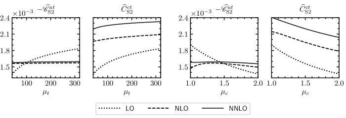
Figure 1: Comparison of Wilson coefficients in $u$-$t$ ($1^{\text{st}}$ and $3^{\text{rd}}$ plot) and $c$-$t$ unitarity ($2^{\text{nd}}$ and $4^{\text{th}}$ plot). Shown is the residual renormalization-scale dependence of the RI Wilson coefficients as a proxy for their theory uncertainty. In the two plots on the left the five-flavour threshold, $\mu_{t}$, is varied, while in the two on the right the three-flavour threshold, $\mu_{c}$, is varied (see text for further details).

In Sec. II we extracted all the necessary quantities to evaluate the $\lambda_{t}^{2}$ and $\lambda_{u}\lambda_{t}$ contributions to $\epsilon_{K}$ at NLL and NNLL accuracy, respectively. Here, we discuss the residual theory uncertainties in $u$-$t$ unitarity and compare them to the traditional approach of $c$-$t$ unitarity. To estimate the uncertainty from missing, higher-order perturbative corrections we vary the unphysical thresholds $\mu_{t}$, $\mu_{b}$, and $\mu_{c}$ in the ranges $40\,\text{GeV}\!\leq\!\mu_{t}\!\leq\!320\,\text{GeV}$, $2.5\,\text{GeV}\!\leq\!\mu_{b}\!\leq\!10\,\text{GeV}$, and $1\,\text{GeV}\!\leq\!\mu_{t}\!\leq\!2\,\text{GeV}$. When varying one scale we keep the other two scales fixed at the values of the RI mass of the fermions, $\mu_{i}=m_{i}(m_{i})$ with $i=t,b,c$. The central values for the $\eta$ parameters are obtained as the average between the lowest and highest value of the three scale variations, and their scale uncertainty as half the difference of the two values. The leading, but small, parametric uncertainties of $\alpha_{s}$ and $m_{c}$ are obtained by varying the parameters at their respective $1\sigma$ ranges. We find

$$\eta_{tt}^{\rm NLL} =\phantom{0}0.55(1\pm 4.2\%_{\text{scales}}\pm 0.1\%_{\alpha_{s}})\,,$$ (16)

$$\eta_{ut}^{\rm NNLL} =0.402(1\pm 1.3\%_{\text{scales}}\pm 0.2\%_{\alpha_{s}}\pm 0.2\%_{m_{c}})\,.$$

Apart from the tiny correction of ${\cal O}(m_{c}^{2}/M_{W}^{2})\sim 10^{-4}$ $\eta_{tt}$ is not affected by the different choice of CKM unitarity. The difference in the scale uncertainty with respect to Ref. Buras et al. (1990) is mainly due to the larger range of scale variation chosen here. By contrast, the residual scale uncertainty of $\eta_{ut}$ is significantly less than the corresponding one in $\eta_{ct}$ and $\eta_{ct}$ in $c$-$t$ unitarity. To illustrate this, we show in Fig. 1 the RI invariant Wilson coefficients $\widehat{\mathscr{C}}^{ut}$ and $\widehat{C}^{ct}$ as a function of the unphysical thresholds $\mu_{t}$ (left two panels) and $\mu_{c}$ (right two panels).

To obtain the standard-model prediction for $\epsilon_{K}$ we employ the Wolfenstein parameterization Tanabashi et al. (2018) of the CKM factors in Eq. (4). In the leading approximation we find $\text{Im}(\lambda_{t}^{2})=-2\lambda^{10}A^{4}\bar{\eta}(1-\bar{\rho})+{\mathcal{O}}(\lambda^{12})$ and $\text{Im}(\lambda_{u}\lambda_{t})=\lambda^{6}A^{2}\bar{\eta}+{\mathcal{O}}(\lambda^{10})$. Numerically, the neglected terms amount to sub-permil effects and can be safely neglected. Therefore, we can use the phenomenological expression (cf. Refs. Buchalla et al. (1996); Buras and Guadagnoli (2008); Buras et al. (2010))

$$\begin{split}|\epsilon_{K}|=&\kappa_{\epsilon}C_{\epsilon}\widehat{B}_{K}|V_{cb}|^{2}\lambda^{2}\bar{\eta}\\ &\times\Big{(}|V_{cb}|^{2}(1-\bar{\rho})\eta_{tt}\mathscr{S}(x_{t})-\eta_{ut}\mathscr{S}(x_{c},x_{t})\Big{)}\,,\end{split}$$ (17)

where

$$C_{\epsilon}=\frac{G_{\rm F}^{2}F_{K}^{2}M_{K^{0}}M_{W}^{2}}{6\sqrt{2}\pi^{2}\Delta M_{K}}\,.$$ (18)

We write $\bar{\eta}=R_{t}\sin\beta$ and $1-\bar{\rho}=R_{t}\cos\beta$, with the quantity $R_{t}$ given by

$$R_{t}\approx\frac{\xi_{s}}{\lambda}\sqrt{\frac{M_{B_{s}}}{M_{B_{d}}}}\sqrt{\frac{\Delta M_{d}}{\Delta M_{s}}}\,.$$ (19)

Here, $\xi_{s}=(F_{B_{s}}\sqrt{\widehat{B}_{s}})/(F_{B_{d}}\sqrt{\widehat{B}_{d}})=1.206(17)$ is a ratio of $B$-meson decay constants and bag factors that is computed on the lattice Aoki et al. (2019). The kaon bag parameter is given by $\widehat{B}_{K}=0.7625(97)$ Aoki et al. (2019). The phenomenological parameter $\kappa_{\epsilon}=0.94(2)$ Buras et al. (2010) comprises long-distance contributions not included in $B_{K}$. As input for the top-quark mass we use RI $\overline{\rm MS}$ mass $m_{t}(m_{t})=163.48(86)\,$GeV. We obtain it by converting the pole mass $M_{t}=173.1(9)\,$GeV Tanabashi et al. (2018) to $\overline{\rm MS}$ at three-loop accuracy using RunDec Chetyrkin et al. (2000). All remaining numerical input is taken from Ref. Tanabashi et al. (2018).

Using the $\eta$ values in Eq. (16) and adding errors in quadrature we find the standard-model prediction

$$\begin{split}|\epsilon_{K}|&=\big{(}2.161\pm 0.153_{\text{param.}}\pm 0.064_{\eta_{tt}}\pm 0.008_{\eta_{ut}}\\ &\qquad\pm 0.027_{\widehat{B}_{K}}\pm 0.052_{\xi_{s}}\pm 0.046_{\kappa_{\epsilon}}\big{)}\times 10^{-3}\,,\\ &=\big{(}2.161\pm 0.153_{\text{param.}}\\ &\qquad\pm 0.076_{\text{non-pert.}}\pm 0.065_{\text{pert.}}\big{)}\times 10^{-3}\,,\\ &=2.16(18)\times 10^{-3}\,.\end{split}$$ (20)

We see that the perturbative uncertainty ($\sim\!\!3.0\%$) is now of the same order as the combined non-perturbative one ($\sim\!\!3.5\%$), while the dominant uncertainties originate from the parametric, experimental uncertainties ($\sim\!\!7.1\%$). Moreover, the dominant perturbative uncertainty no longer originates from $\eta_{ct}$ but from the top-quark contribution, $\eta_{tt}$.

IV Discussion and Conclusions

In this letter, we showed that a manifest implementation of CKM unitarity in the effective $|\Delta{\rm S}\!=\!2|$ Hamiltonian dramatically improves the convergence behaviour of the perturbative series for its imaginary part, by removing a spurious long-distance charm-quark contribution. In this way, and using only known results in the literature, we reduced the residual uncertainty of the short-distance charm-quark contribution to the weak Hamiltonian by more than an order of magnitude. The perturbative uncertainty is now dominated by the missing NNLO corrections to the top-quark contribution, as well as partially known electroweak corrections at the percent level (see Refs. Gambino et al. (1999); Brod and Gorbahn (2008); Brod et al. (2011)). The calculation of these corrections Brod et al. (work in progress) has the potential to bring the perturbative uncertainty of $\epsilon_{K}$ down to the percent level, motivating a renewed effort to compute long-distance effects using lattice QCD.

By contrast, the real part of the $|\Delta{\rm S}\!=\!2|$ Hamiltonian is dominated by up- and charm-quark contributions, and their convergence is not improved. Hence, the calculation of these contributions is a genuine task for lattice QCD, to which a significant effort is devoted Christ et al. (2013); Bai et al. (2014); Blum et al. (2015). However, our results have the potential to supply useful cross checks for part of these calculations: By performing the matching to the hadronic matrix elements for $\epsilon_{K}$ above the charm-quark threshold we can obtain a prediction of these matrix elements that can be directly compared to a future lattice calculation. This could shed additional light onto the lattice calculation of the kaon mass difference.

References

Anikeev et al. (2001)
K. Anikeev et al.,
in Workshop on B Physics at the Tevatron: Run II
and Beyond Batavia, Illinois, September 23-25, 1999
(2001), eprint hep-ph/0201071,
URL http://lss.fnal.gov/cgi-bin/find_paper.pl?pub-01-197.
Christ et al. (2013)
N. H. Christ,
T. Izubuchi,
C. T. Sachrajda,
A. Soni, and
J. Yu
(RBC, UKQCD), Phys. Rev.
D88, 014508
(2013), eprint 1212.5931.
Buchalla et al. (1996)
G. Buchalla,
A. J. Buras, and
M. E. Lautenbacher,
Rev. Mod. Phys. 68,
1125 (1996), eprint hep-ph/9512380.
Herrlich and Nierste (1996)
S. Herrlich and
U. Nierste,
Nucl. Phys. B476,
27 (1996), eprint hep-ph/9604330.
Brod and Gorbahn (2012)
J. Brod and
M. Gorbahn,
Phys. Rev. Lett. 108,
121801 (2012), eprint 1108.2036.
Brod and Gorbahn (2010)
J. Brod and
M. Gorbahn,
Phys. Rev. D82,
094026 (2010), eprint 1007.0684.
Inami and Lim (1981)
T. Inami and
C. S. Lim,
Prog. Theor. Phys. 65,
297 (1981), [Erratum: Prog.
Theor. Phys.65,1772(1981)].
Buras et al. (1990)
A. J. Buras,
M. Jamin, and
P. H. Weisz,
Nucl. Phys. B347,
491 (1990).
Buras et al. (1992)
A. J. Buras,
M. Jamin,
M. E. Lautenbacher,
and P. H. Weisz,
Nucl. Phys. B370,
69 (1992), [Addendum: Nucl.
Phys.B375,501(1992)].
Bobeth et al. (2000)
C. Bobeth,
M. Misiak, and
J. Urban,
Nucl. Phys. B574,
291 (2000), eprint hep-ph/9910220.
Buras et al. (2006)
A. J. Buras,
M. Gorbahn,
U. Haisch, and
U. Nierste,
JHEP 11, 002
(2006), [Erratum: JHEP11,167(2012)],
eprint hep-ph/0603079.
Witten (1977)
E. Witten,
Nucl. Phys. B122,
109 (1977).
Herrlich and Nierste (1994)
S. Herrlich and
U. Nierste,
Nucl. Phys. B419,
292 (1994), eprint hep-ph/9310311.
Tanabashi et al. (2018)
M. Tanabashi
et al. (Particle Data Group),
Phys. Rev. D98,
030001 (2018).
Buras and Guadagnoli (2008)
A. J. Buras and
D. Guadagnoli,
Phys. Rev. D78,
033005 (2008), eprint 0805.3887.
Buras et al. (2010)
A. J. Buras,
D. Guadagnoli,
and G. Isidori,
Phys. Lett. B688,
309 (2010), eprint 1002.3612.
Aoki et al. (2019)
S. Aoki et al.
(Flavour Lattice Averaging Group)
(2019), eprint 1902.08191.
Chetyrkin et al. (2000)
K. G. Chetyrkin,
J. H. Kuhn, and
M. Steinhauser,
Comput. Phys. Commun. 133,
43 (2000), eprint hep-ph/0004189.
Gambino et al. (1999)
P. Gambino,
A. Kwiatkowski,
and N. Pott,
Nucl. Phys. B544,
532 (1999), eprint hep-ph/9810400.
Brod and Gorbahn (2008)
J. Brod and
M. Gorbahn,
Phys. Rev. D78,
034006 (2008), eprint 0805.4119.
Brod et al. (2011)
J. Brod,
M. Gorbahn, and
E. Stamou,
Phys. Rev. D83,
034030 (2011), eprint 1009.0947.
Brod et al. (work in progress)
J. Brod,
M. Gorbahn,
E. Stamou, and
H. Yu (work in
progress).
Bai et al. (2014)
Z. Bai,
N. H. Christ,
T. Izubuchi,
C. T. Sachrajda,
A. Soni, and
J. Yu, Phys.
Rev. Lett. 113, 112003
(2014), eprint 1406.0916.
Blum et al. (2015)
T. Blum et al.,
Phys. Rev. D91,
074502 (2015), eprint 1502.00263.