Non-Monotone Submodular Maximization with Multiple Knapsacks in Static and Dynamic Settings.

Abstract

We study the problem of maximizing a non-monotone submodular function under multiple knapsack constraints. We propose a simple discrete greedy algorithm to approach this problem, and prove that it yields strong approximation guarantees for functions with bounded curvature. In contrast to other heuristics, this does not require problem relaxation to continuous domains and it maintains a constant-factor approximation guarantee in the problem size. In the case of a single knapsack, our analysis suggests that the standard greedy can be used in non-monotone settings.

Additionally, we study this problem in a dynamic setting, in which knapsacks change during the optimization process. We modify our greedy algorithm to avoid a complete restart at each constraint update. This modification retains the approximation guarantees of the static case.

We evaluate our results experimentally on a video summarization and sensor placement task. We show that our proposed algorithm competes with the state-of-the-art in static settings. Furthermore, we show that in dynamic settings with tight computational time budget, our modified greedy yields significant improvements over starting the greedy from scratch, in terms of the solution quality achieved.

1 INTRODUCTION

Many artificial intelligence and machine learning tasks can be naturally approached by maximizing submodular objectives. Examples include subset selection [10], document summarization [24], video summarization [26] and action recognition [37]. Submodular functions are set functions that yield a diminishing return property: it is more helpful to add an element to a smaller collection than to add it to a larger one. This property fully characterizes the notion of submodularity.

Practical applications often require additional side constraints on the solution space, determined by possible feasibility conditions. These constraints can be complex [24, 28, 35]. For instance, when performing video summarization tasks, we might want to select frames that fulfill costs constraints based on qualitative factors, such as resolution and luminance.

In this paper, we study general multiple knapsack constraints. Given a set of solutions, a $k$-knapsack constraint consists of $k$ linear cost functions $c_{i}$ on the solution space and corresponding weights $W_{i}$. A solution is then feasible if the corresponding costs do not exceed the weights. In this paper, we study the problem of maximizing a submodular function under a $k$-knapsack constraint.

Sometimes, real-world optimization problems involve dynamic and stochastic constraints [6]. For instance, resources and costs can exhibit slight frequent changes, leading to changes of the underlying space of feasible solutions. Various optimization problems have been studied under dynamically changing constraints, i.e., facility location problems [17], target tracking [13], and other submodular maximization problems for machine learning [4]. Motivated by these applications, we also study the problem of maximizing a submodular function under a $k$-knapsack constraint, when the set of feasible solutions changes online.

Literature Overview.

Khuller, Moss and Naor [18] show that a simple greedy algorithm achieves a $1/2(1-1/e)$-approximation guarantee, when maximizing a modular function with a single knapsack constraint. They also propose a modified greedy algorithm that achieves a $(1-1/e)$-approximation. Sviridenko [32] shows that this modified greedy algorithm yields a $(1-1/e)$-approximation guarantee for monotone submodular functions under a single knapsack constraint. Its run time is $O(n^{5})$ function evaluations. The optimization of monotone submodular functions under a given chance constraint by an adaptation of these simple greedy algorithm has recently been investigated by Doerr et al. [11].

Lee et al. [23] give a $(1/5-\varepsilon)$-approximation local search algorithm, for maximizing a non-monotone submodular function under multiple knapsack constraints. Its run time is polynomial in the problem size and exponential in the number of constraints. Fadaei, Fazli and Safari [12] propose an algorithm that achieves a ($1/4-\varepsilon$)-approximation algorithm for non-monotone functions. This algorithm requires to compute fractional solutions of a continuous extension of the value oracle function $f$. Chekuri, Vondrák and Zenklusen [5] improve the approximation ratio to $0.325-\varepsilon$, in the case of $k=\mathcal{O}\left(1\right)$ knapsacks. Kulik, Schachnai and Tamir [22] give a $(1-1/e-\varepsilon)$-approximation algorithm when $f$ is monotone and a $(1/e-\varepsilon)$-approximation algorithm when the function is non-monotone. Again, their method uses continuous relaxations of the discrete setting. Fantom is a popular algorithm for non-monotone submodular maximization [27]. It can handle intersections of a variety of constraints. In the case of multiple knapsack constraints, it achieves a $1/((1+\varepsilon)(10+4k))$-approximation in $\mathcal{O}\left(n^{2}\log(n)/\varepsilon\right)$ run time.

Submodular optimization problems with dynamic cost constraints, including knapsack constraints, are investigated in [30, 31]. Rostapoor et al. [31] show that a Pareto optimization approach can implicitly deal with dynamically changing constraint bounds, whereas a simple adaptive greedy algorithm fails.

Our Contribution.

Many of the aforementioned algorithmic results, despite having polynomial run time, seem impractical for large input applications. Following the analysis outlined in [8, 15, 18], we propose a simple and practical discrete algorithm to maximize a submodular function under multiple knapsack constraints. This algorithm, which we call the $\lambda$-Greedy, achieves a $(1-e^{-1/\lambda})/(3\max(1,\alpha))$-approximation guarantee on this problem, with $\alpha$ expressing the curvature of $f$, and $\lambda\in[1,k]$ a constant. It requires at most $\mathcal{O}(n^{\max(k/\lambda,2)})$ function evaluations. To our knowledge this is the first algorithm yielding a trade-off between run-time and approximation ratio.
We also propose a robust variation of our $\lambda$-Greedy, which we call $\lambda$-dGreedy, to handle dynamic changes in the feasibility region of the solution space. We show that this algorithm maintains a $(1-e^{-1/\lambda})/(3\max(1,\alpha))$-approximation without having to do a complete restart of the greedy sequence.

We demonstrate experimentally that our algorithms yield good performance in practise, with two real-world scenarios. First, we consider a video summarization task, which consists of selecting representative frames of a given video [28, 27]. We also consider a sensor placement problem, that asks to select informative thermal stations over a large territory [19].
Our experiments indicate that the $\lambda$-Greedy yields superior performance to commonly used algorithms for the static video summarization problem. We then perform experiments in dynamic settings with both scenarios, to show that the robust variation yields significant improvement in practise.

The paper is structured as follows. In Section 2 we introduce basic definitions and define the problem. In Section 3 we define the algorithms. We present the theoretical analysis in Section 4, and the experimental framework in Section 5. The experimental results are discussed in Section 6 and Section 7. We conclude in Section 8.

2 PRELIMINARIES

Submodularity and Curvature

In this paper, we consider problems with an oracle function that outputs the quality of given solution. We measure performance in terms of calls to this function, since in many practical applications they are difficult to evaluate. We assume that value oracle functions are submodular, as in the following definition.

Definition (Submodularity)

Given a finite set $V$, a set function $f\colon 2^{V}\rightarrow\mathbb{R}$ is submodular if for all $S,\Omega\subseteq V$ we have that $f(S)+f(\Omega)\geq f(S\cup\Omega)+f(S\cap\Omega)$.

For the equivalent intuitive definition described informally in the introduction see [29].

For any submodular function $f\colon 2^{V}\rightarrow\mathbb{R}$ and sets $S,\Omega\subseteq V$, we define the marginal value of $\Omega$ with respect to $S$ as $f_{S}(\Omega)=f(S\cup\Omega)-f(S)$. Note that, if $f$ only attains non-negative values, it holds that $f(\Omega)\geq f_{S}(\Omega)$ for all $S,\Omega\subseteq V$.

Our approximation guarantees use the notion of curvature, a parameter that bounds the maximum rate with which a submodular function changes. We say that a submodular function $f\colon 2^{V}\rightarrow\mathbb{R}_{\geq 0}$ has curvature $\alpha$ if the value $f(S\cup e)-f(S)$ does not change by a factor larger than $1-\alpha$ when varying $S$, for all $e\in V\setminus S$. This parameter was first introduced by [8] and later revisited in [3]. We use the following definition of curvature, which slightly generalizes that proposed in Friedrich et al. [15].

Definition (Curvature)

Let $f\colon 2^{V}\rightarrow\mathbb{R}_{\geq 0}$ be a submodular set function. The curvature is the smallest scalar $\alpha$ such that

$$f_{\omega}((S\cup\Omega)\setminus\{\omega\})\geq(1-\alpha)f_{\omega}(S\setminus\{\omega\}),$$

for all $S,\Omega\subseteq V$ and $\omega\in S\setminus\Omega$.

Note that $\alpha\leq 1$ always holds and that all monotone submodular functions have curvature always bounded as $0\leq\alpha\leq 1$. It follows that all submodular functions with negative curvature are non-monotone.

Problem Description

The problem of maximizing a submodular function under multiple knapsack constraints can be formalized as follows.

Problem

Let $f\colon 2^{V}\rightarrow\mathbb{R}_{\geq 0}$ be a submodular function. Consider linear cost functions $c_{i}\colon 2^{V}\rightarrow\mathbb{R}_{\geq 0}$, and corresponding weights $W_{i}$, for all $i\in[k]$. We search for a set $\textsc{opt}\subseteq V$, such that $\textsc{opt}\in\operatorname*{arg\,max}_{S\subseteq V}\left\{f(S)\colon c_{i}(S)\leq W_{i},\forall i\in[k]\right\}$.

In this setting, one has $k$ knapsacks and wishes to find an optimal set of items such that its total cost, expressed by the functions $c_{i}$, does not violate the capacity of each knapsack. Note that the same set might have different costs for different knapsacks.
We denote with $(c,W)$ the constraint requirements $c_{i}(S)\leq W_{i}$ for all $S\subseteq V$, for all $i\in[k]$. For a ground set $V$ with a fixed ordering on the points and a cost function $c_{i}$, where $i\in[k]$, let $\tau_{i}$ be a permutation on $V$ where $c_{i}(e_{\tau_{i}(1)})\geq\dots\geq c_{i}(e_{\tau_{i}(n)})$. We define the value $\chi(c,W)$ as

$$\chi(c,W)=\min_{i\in[k]}\operatorname*{arg\,max}_{j\in[\left\lvert V\right\rvert]}\left\{\sum_{\ell=1}^{j}c_{i}(e_{\tau_{i}(\ell)})\leq W_{i}\right\}.$$

Note that the value $\chi(c,W)$ is such that each set $U\subseteq V$ with cardinality $\left\lvert U\right\rvert\leq\chi(c,W)$ is feasible for all constraints in $(c,W)$.
We observe that in the case of a single knapsack, if $c_{1}(S)=\left\lvert S\right\rvert$ for all $S\subseteq V$, then Problem 2 consists of maximizing a submodular function under a cardinality constraint, which is known to be NP-hard.

In our analysis we always assume that the following reduction holds.

Reduction

For Problem 2 we may assume that there exists a point $e^{*}\in V$ such that $f(S\cup e^{*})=f(S)$ for all $S\subseteq V$, and $c_{i}(e^{*})=W_{i}$ for all $i\in[k]$. Furthermore, we may assume that $c_{i}(e)\leq W_{i}$ for all $e\in V$, for all $i\in[m]$.

If the conditions of Reduction 2 do not hold, one can remove all points $e\in V$ that violate one of the constraints and add a point $e^{*}$ without altering the function $f$. Intuitively, Reduction 2 requires that each singleton, except for one, is feasible for all knapsack constraints. This ensures that $\operatorname*{arg\,max}_{e\in V}f(e)$ is always feasible in all constraints, since $f(e^{*})=0$, and the optimum solution consists of at least one point. Furthermore, the point $e^{*}\in V$ ensures that the solution quality never decreases throughout a greedy optimization process, until a non-feasible solution is reached.

Additionally, we study a dynamic setting of Problem 2, in which weights $W_{i}$ are repeatedly updated throughout the optimization process, while the corresponding cost functions $c_{i}$ remain unchanged. In this setting, we assume that an algorithm queries a function to retrieve the weights $W_{i}$ which are, sometimes, updated online. We assume that weights changes occur independently of the optimization process and algorithmic operations. Furthermore, we assume that Reduction 2 holds for each dynamic update.

3 ALGORITHMS

input: submodular function $f$, $k$-knapsacks $(c,W)$ and parameter $\lambda$ ;

output: an approximate feasible global maximum of $f$;

$\mathcal{V}\leftarrow\{e\in V\colon c_{j}(e)\leq\lambda W_{j}/k\ \forall j\in[k]\}$;

$S\leftarrow\mathcal{V}$;

$\sigma\leftarrow\emptyset$;

$v^{*}\leftarrow\operatorname*{arg\,max}_{e\in V}f(e)$;

while $S\neq\emptyset$ do

       let $e\in S$ maximizing $f_{\sigma}(e)/\max_{j}c_{j}(e)$;

       $S\leftarrow S\setminus e$;

       if $c_{j}(\sigma\cup e)\leq W_{j},\forall j\in[k]$ then $\sigma\leftarrow\sigma\cup e$;

      

return $\operatorname*{arg\,max}_{\{U\subseteq V\setminus\mathcal{V}\colon c_{i}(U)\leq W_{i}\ \forall i\}}\{f(\sigma),f(v^{*}),f(U)\}$;

Algorithm 1 The $\lambda$-Greedy algorithm.

input: submodular function $f$, $k$-knapsacks $(c,W)$ with dynamic weights and parameter $\lambda$;

output: an approximate feasible global maximum of $f$;

evaluate $f$ over all sets of cardinality at most $k/\lambda$;

$\mathcal{V}\leftarrow\{e\in V\colon c_{j}(e)\leq\lambda W_{j}/k\ \forall j\in[k]\}$;

$S\leftarrow\mathcal{V}$;

$\sigma\leftarrow\emptyset$;

$v^{*}\leftarrow\operatorname*{arg\,max}_{e\in V}f(e)$;

while $S\neq\emptyset$ do

         

       // greedy rule

       let $e\in S$ maximizing $f_{\sigma}(e)/\max_{j}c_{j}(e)$;

       $S\leftarrow S\setminus e$;

       if $c_{i}(\sigma\cup e)\leq W_{i},\forall i\in[k]$ then $\sigma\leftarrow\sigma\cup v$;

         

       // update rule

       if new weights $\{W_{i}^{\prime}\}$ are given then

             $\mathcal{V}^{\prime}\leftarrow\{e\in V\colon c_{j}(e)\leq\lambda W^{\prime}_{j}/k\ \forall j\in[k]\}$;

             while $\left\lvert\sigma\right\rvert>\min\{\chi(c,W),\chi(c,W^{\prime})\}\lor\sigma\not\subseteq\mathcal{V}\cap\mathcal{V}^{\prime}$  do

                   let $e\in\sigma$ be the last point added to $\sigma$;

                   $\sigma\leftarrow\sigma\setminus e$;

                  

            $\mathcal{V}\leftarrow\mathcal{V}^{\prime}$;

             $S\leftarrow\mathcal{V}\setminus\sigma$;

            

      

return $\operatorname*{arg\,max}_{\{U\subseteq V\setminus\mathcal{V}\colon c_{i}(U)\leq W\ \forall i\}}\{f(\sigma),f(v^{*}),f(U)\}$;

Algorithm 2 The $\lambda$-dGreedy algorithm.

We approach Problem 2 with a discrete algorithm based on a greedy technique, commonly used to maximize a submodular function under a single knapsack constraint (see [18, 36]). Given the parameter value $\lambda\in[k]$, our algorithm defines the following partition of the objective space:

1. the set $\mathcal{V}$ containing all $e\in V$ such that $c_{j}\leq\lambda W_{j}/k$ for all $j\in[k]$;

2. the complement $V\setminus\mathcal{V}$ containing all $e\in\mathcal{V}$ such that $c_{j}(e)>\lambda W_{j}/k$ for all $j\in[k]$.

The $\lambda$-Greedy optimizes $f$ over the set $\mathcal{V}$, with a greedy update that depends on all cost functions $c_{j}$. After finding a greedy approximate solution $\sigma$, the $\lambda$-Greedy finds the optimum $\tau$ among feasible subsets of $V\setminus\mathcal{V}$. This step can be performed with a deterministic search over all possible solutions, since the space $V\setminus\mathcal{V}$ always has bounded size. The $\lambda$-Greedy outputs the set with highest $f$-value among $\sigma,\tau$ or the maximum among the singletons.

From the statement of Theorem 4.1 we observe that the parameter $\lambda$ sets a trade-off between solution quality and run time. For small $\lambda$, Algorithm 1 yields better approximation guarantee and worse run time, than for large $\lambda$. This is due to the fact that the size of $\mathcal{V}\setminus V$ depends on this parameter. In practise, the parameter $\lambda$ allows to find the right trade-off between solution quality and run time, depending on available resources. Note that in the case of a single knapsack constraint, for $\lambda=k$ the $\lambda$-Greedy is equivalent to the greedy algorithm studied in [18].

We modify the $\lambda$-Greedy to handle dynamic constraints where weights change overtime. This algorithm, which we refer to as the $\lambda$-dGreedy, is presented in Algorithm 2. It consists of two subroutines, which we call the greedy rule and the update rule. The greedy rule of the $\lambda$-dGreedy uses the same greedy update as the $\lambda$-Greedy does: At each step, find a point $v\in V$ that maximizes the marginal gain over maximum cost, and add $v$ to the current solution, if the resulting set is feasible in all knapsacks. The update rule allows to handle possible changes to the weights, even when the greedy procedure has not terminated, without having to completely restart the algorithm.

Following the notation of Algorithm 2, if new weights $W^{\prime}_{1},\dots,W^{\prime}_{k}$ are given, then the $\lambda$-dGreedy iteratively removes points from the current solution, until the resulting set yields $\sigma\leq\min\{\chi(c,W),\chi(c,W^{\prime})\}$ and $\sigma\subseteq\mathcal{V}\cap\mathcal{V}^{\prime}$. This is motivated by the following facts:

1. every set $U\leq\min\{\chi(c,W),\chi(c,W^{\prime})\}$ is feasible in both the old and the new constraints;

2. every set $U\leq\min\{\chi(c,W),\chi(c,W^{\prime})\}$ such that $U\subseteq\mathcal{V}\cap\mathcal{V}^{\prime}$ obtained with a greedy procedure yields the same approximation guarantee in both constraints;

3. every set $U\subseteq\mathcal{V}\cap\mathcal{V}^{\prime}$ is such that $c_{i}(e)\leq\lambda W^{\prime}_{i}/k$ for all $i\in k$, for all $e\in U$.

All three conditions are necessary to ensure that the approximation guarantee is maintained.

Note that the update rule in Algorithm 2 does not backtrack the execution of the algorithm until the resulting solution is feasible in the new constraint, and then adds elements to the current solution. For instance, consider the following example, due to Roostapour et al. [31]. We are given a set of $n+1$ items $\{e_{1},\dots,e_{n+1}\}$ under a single knapsack $(c,W)$, with the cost function $c$ defined as

$$c(e_{i})=\left\{\begin{array}[]{ll}1,&\mbox{if }1\leq i\leq n/2\mbox{ or }i=n+1;\\ 2,&\mbox{otherwise};\\ \end{array}\right.$$

and $f$-values defined on the singleton as

$$f(e_{i})=\left\{\begin{array}[]{ll}1/n,&\mbox{if }1\leq i\leq n/2;\\ 1,&\mbox{if }n/2<i\leq n;\\ 3,&\mbox{if }i=n+1;\\ \end{array}\right.$$

We define $f(U)=\sum_{e\in U}f(e)$, for all $U\subseteq\{e_{1},\dots,e_{n+1}\}$. Consider Algorithm 2 optimizing $f$ from scratch with $W=2$. We only consider the case $\lambda=1$, since we only consider a single knapsack constraint. Then both Algorithm 2 and the $\lambda$-Greedy return a set of the form $\{e_{n+1},e_{j}\}$ with $1\leq j\leq n/2$. Suppose now that the weight dynamically changes to $W=3$. Then backtracking the execution and adding points to the current solution would result into a solution of the form $\{e_{n+1},e_{i},e_{j}\}$ with $1\leq i,j\leq n/2$ with $f(\{e_{n+1},e_{i},e_{j}\})=3+2/n$. However, in this case it holds $\min\{\chi(c,2),\chi(c,3)\}=1$, since there exists a solution of cardinality $2$ that is not feasible in $(c,2)$. Hence, Algorithm 2 removes the point $e_{j}$ from the solution $\{e_{n+1},e_{j}\}$, before adding new elements to it. Afterwards, it adds a point $e_{j^{\prime}}$ with $n/2<{j^{\prime}}\leq n$ to it, obtaining a solution such that $f(\{e_{n+1},e_{j^{\prime}}\})=3+1=4$.
We remark that on this instance, the $\lambda$-Greedy with a simple backtracking operator yields arbitrarily bad approximation guarantee, as discussed in [31, Theroem 3]. In contrast, Algorithm 2 maintains the approximation guarantee on this instance (see Theorem 4.2).

4 APPROXIMATION GUARANTEES

We prove that Algorithm 1 yields a strong approximation guarantee, when maximizing a submodular function under $k$ knapsack constraints in the static case. This part of the analysis does not consider dynamic weight updates. We use the notion of curvature as in Definition 2.

Theorem 4.1.

Let $f$ be a submodular function with curvature $\alpha$, suppose that $k$ knapsacks are given. For all $\lambda\in[1,k]$, the $\lambda$-Greedy is a $(1-e^{-1/\lambda})/(3\max(1,\alpha))$-approximation algorithm for Problem 2. Its run time is $\mathcal{O}\left(n^{\max(k/\lambda,2)}\right)$.

This proof is based on the work of Khuller et al. [18]. Note that if the function $f$ is monotone, then the approximation guarantee given in Theorem 4.1 matches well-known results [18]. We remark that non-monotone functions with bounded curvature are not uncommon in practise. For instance, all cut functions of directed graphs are non-monotone, submodular and have curvature $\alpha\leq 2$, as discussed in [15].

We perform the run time analysis for the $\lambda$-Greedy in dynamic settings, in which weights $\{W_{i}\}_{i}$ change over time.

Theorem 4.2.

Consider Algorithm 2 optimizing a submodular function with curvature $\alpha>0$ and knapsack constraints $(c,W)$. Suppose that at some point during the optimization process new weights $W^{\prime}_{i}$ are given. Let $\sigma$ be the current solution before the weights update, and let $\sigma_{t}\subseteq\sigma$ consist of the first $t$ points added to $\sigma$. Furthermore, let $t^{*}$ be the largest index such that $\sigma_{t^{*}}\subseteq\mathcal{V}\cap\mathcal{V}^{\prime}$, with $\mathcal{V},\mathcal{V}^{\prime}$ as in Algorithm 2, and define $\chi=\min\left\{\chi(c,W),\chi(c,W^{\prime}),t^{*}\right\}.$ Then after additional $\mathcal{O}\left(n(n-\chi)\right)$ run time the $\lambda$-Greedy finds a $(1-e^{-1/\lambda})/(3\max(1,\alpha))$-approximate optimal solution in the new constraints, for a fixed parameter $\lambda\in[1,k]$.

Intuitively, this proof shows that, given two sets of feasible solutions $\mathcal{V},\mathcal{V}^{\prime}$, the $\lambda$-Greedy follows the same paths on both problem instances, for all solutions with size up to $\chi$. Note that Theorem 4.1 yields the same theoretical approximation guarantee as Theorem 4.2. Hence, if dynamic updates occur at a slow pace, it is possible to obtain identical results by restarting $\lambda$-Greedy every time a constraint update occurs. However, as we show in Section 7, there is significant advantage in using the $\lambda$-dGreedy in settings when frequent noisy constraints updates occur.

5 APPLICATIONS

In this section we present a high-level overview of two possible applications for Problem 2. We describe experimental frameworks and implementations for these applications in Sections 6-7.

Video Summarization.

Determinantal Point Process (DPP), [25], is a probabilistic model, the probability distribution function of which can be characterized as the determinant of a matrix. More formally, consider a sample space $V=[n]$, and let $L$ be a positive semidefinite matrix. We say that $L$ defines a DPP on $V$, if the probability of an event $S\subseteq V$ is given by

$$\mathcal{P}_{L}(S)=\frac{\det(L_{S})}{\det(L+I)},$$

where $L_{S}=(L_{i,j})_{i,j\in S}$ is the submatrix of $L$ indexed by the elements in $S$, and $I$ is the $n\times n$ identity matrix. For a survey on DPPs and their applications see [21].

We model this framework with a matrix $L$ that describes similarities between pairs of frames. Intuitively, if $L$ describes the similarity between two frames, then the DPP prefers diversity.
In this setting, we search for a set of features $S\subseteq V$ such that $\mathcal{P}(S)$ is maximal, among sets of feasible solutions defined in terms of a knapsack constraint. Since $L$ is positive semidefinite, the function $\log\det L_{S}$ is submodular [21].

Sensor Placement.

The maximum entropy sampling problem consists of choosing the most informative subset of random variables subject to side constraints. In this work, we study the problem of finding the most informative set among given Gaussian time series.

Given a sample covariance matrix $\Sigma$ of the time series corresponding to measurements, the entropy of a subset of sensors is then given by the formula

$$f(S)=\frac{1+\ln(2\pi)}{2}\left\lvert S\right\rvert+\frac{1}{2}\ln\det(\Sigma_{S})$$

for any indexing set $S\subseteq\{0,1\}^{n}$ on the variation series, where $\det(\Sigma_{S})$ returns the determinant of the sub-matrix of $\Sigma$ indexed by $S$. It is well-known that the function $f$ is non-monotone and submodular. Its curvature is bounded as $\alpha\leq 1-1/\mu$, where $\mu$ is the largest eigenvalue of $\Sigma$ [33, 19, 15].
We consider the problem of maximizing the entropy $f$ under a partition matroid constraint. This additional side constraint requires upper-bounds on the number of sensors that can be chosen in given geographical areas.

6 STATIC EXPERIMENTS

		run time for each video clip
algorithm	parameter	video (1)	video (2)	video (3)	video (4)	video (5)	video (6)	video (7)
Fantom	$\varepsilon=0.001$	4085317	3529230	3813637	2986719	3368901	3442329	3082814
Fantom	$\varepsilon=0.01$	406960	351321	382342	299444	336670	344619	307726
Fantom	$\varepsilon=0.1$	41008	34309	37232	29249	33343	33146	30235
$\lambda$-Greedy	$\lambda=k$	2895	2895	2895	2709	2895	2709	2522
algorithm	parameter	video (8)	video (9)	video (10)	video (11)	video (12)	video (13)	video (14)
Fantom	$\varepsilon=0.001$	3171467	3781141	3121379	3673776	3603787	3055122	4119203
Fantom	$\varepsilon=0.01$	320738	379420	313975	368617	360265	307399	412247
Fantom	$\varepsilon=0.1$	30605	36608	30809	36242	35682	30223	40543
$\lambda$-Greedy	$\lambda=k$	2709	3080	2895	2895	3080	2709	3080
algorithm	parameter	video (15)	video (16)	video (17)	video (18)	video (19)	video (20)
Fantom	$\varepsilon=0.001$	3727241	3321987	3429387	3555884	3375296	3431653
Fantom	$\varepsilon=0.01$	374322	330994	345333	354694	336718	343419
Fantom	$\varepsilon=0.1$	36073	32377	33357	34741	32370	32187
$\lambda$-Greedy	$\lambda=k$	2895	2895	2895	2895	2709	2709

		solution quality for each video clip
algorithm	parameter	video (1)	video (2)	video (3)	video (4)	video (5)	video (6)	video (7)
Fantom	$\varepsilon=0.001$	19.3818	15.6143	15.4285	10.6228	13.2393	14.0438	9.4999
Fantom	$\varepsilon=0.01$	19.3818	15.6143	15.4285	10.6228	13.2393	12.9851	9.4999
Fantom	$\varepsilon=0.1$	16.9083	13.9868	13.9942	9.1811	13.2393	12.9851	9.4999
$\lambda$-Greedy	$\lambda=k$	23.9323	21.8122	22.5406	15.0203	19.4932	18.6267	15.5678
algorithm	parameter	video (8)	video (9)	video (10)	video (11)	video (12)	video (13)	video (14)
Fantom	$\varepsilon=0.001$	11.0898	16.2864	10.7798	15.9894	15.5939	12.5897	18.7495
Fantom	$\varepsilon=0.01$	11.0898	16.2864	10.7798	15.9894	15.5939	12.5897	18.7495
Fantom	$\varepsilon=0.1$	9.5612	16.2864	10.7798	14.4139	14.1122	9.5909	17.3095
$\lambda$-Greedy	$\lambda=k$	18.5727	23.9619	17.6612	23.2229	20.8876	18.1164	25.1342
algorithm	parameter	video (15)	video (16)	video (17)	video (18)	video (19)	video (20)
Fantom	$\varepsilon=0.001$	16.3391	11.8452	13.6084	16.9964	13.0314	13.0558
Fantom	$\varepsilon=0.01$	16.3391	11.8452	13.6084	16.9964	13.0314	13.0558
Fantom	$\varepsilon=0.1$	14.7544	11.8452	12.0878	14.0999	11.5619	11.5385
$\lambda$-Greedy	$\lambda=k$	23.8740	19.4916	19.9461	22.2884	18.6588	19.0673

Table 1: We consider $20$ movies from the Frames Labeled In Cinema dataset [14]. For each movie, we select a representative set of frames, by maximizing a submodular function under additional knapsack constraints, as described in Section 6. We run the $\lambda$-Greedy and the Fantom algorithm [26] with various parameter choices, until no remaining point in the search space yields improvement on the fitness value, without violating side constraints. We observe that in all cases the $\lambda$-Greedy yields better run time and solution quality than the Fantom.

The aim of these experiments is to show that the $\lambda$-Greedy yields better performance in comparison with Fantom [26], which is a popular algorithm for non-monotone submodular objectives under complex sets of constraints. We consider video summarization tasks as in Section 5.

Let $L$ be the matrix describing similarities between pairs of frames, as in Section 5. Following [16], we parametrize $L$ as follows. Given a set of frames, let $\bm{f}_{i}$ be the feature vector of the $i$-th frame. This vector encodes the contextual information about frame $i$ and its representativeness of other items. Then the matrix $L$ can be paramterized as $L_{i,j}=\bm{z}_{i}^{T}W^{T}W\bm{z}_{j}$, with $\bm{z}_{i}=\tanh(U\bm{f}_{i})$ being a hidden representation of $\bm{f}_{i}$, and $U,W$ parameters. We use a single-layer neural network to train the parameters $U,W$. We consider $20$ movies from the Frames Labeled In Cinema dataset [14]. Each movie has $200$ frames and $7$ generated ground summaries consisting of $15$ frames each.

We select a representative set of frames, by maximizing the function $\log\det L$ under additional quality feature constraints, viewed as multiple knapsacks. Hence, this task consists of maximizing a non-monotone submodular function under multiple knapsack constraints.
We run the $\lambda$-Greedy and Fantom algorithms on each instance, until no remaining point in the search space yields improvement on the fitness value, without violating side constraints. We then compare the resulting run time and empirical approximation ratio. Since Fantom depends on a parameter $\varepsilon$ [26], we perform three sets of experiments for $\varepsilon=0.1$, $\varepsilon=0.01$, and $\varepsilon=0.001$. The parameter $\lambda$ for the $\lambda$-Greedy is always set to $\lambda=k$. We have no indications that a lower $\lambda$ yields improved solution quality on this set of instances.

Results for the run time and approximation guarantee are displayed in Table 1. We clearly see that the $\lambda$-Greedy outperforms Fantom in terms of solution quality. Furthermore, the run time of Fantom is orders of magnitude worse than that of our $\lambda$-Greedy. This is probably due to the fact that the Fantom requires a very low density threshold to get to a good solution on these instances. The code for this set of experiments is available upon request.

7 DYNAMIC EXPERIMENTS

The aim of these experiments is to show that, when constraints quickly change dynamically, the robust $\lambda$-dGreedy significantly outperforms the $\lambda$-Greedy with a restart policy, that re-sets the optimization process each time new weights are given. To this end, we simulate a setting where updates change dynamically, by introducing controlled posterior noise on the weights. At each update, we run the $\lambda$-Greedy from scratch, and let the $\lambda$-dGreedy continue without a restart policy. We consider two set of dynamic experiments.

The Maximum Entropy Sampling Problem

Table 2: For the respective set of experiments, Maximum Entropy Sampling (left) and Video Summarization (right), the mean and standard deviation of the solution quality over time within one run of the respective algorithms for different update frequencies [$\tau$] and different dynamic update standard deviations [$\sigma$]. With $X^{(+)}$ we denote that the algorithm labelled $X$ significantly outperformed the other one.

		$\lambda$-Greedy (1)		$\lambda$-dGreedy (2)
$\tau$	$\sigma$	mean	sd	mean	sd	stat
10K	0.075	107.4085	1.35	$\mathbf{130.5897}$	12.28	$2^{(+)}$
20K	0.075	195.0352	2.99	$\mathbf{213.3886}$	11.15	$2^{(+)}$
30K	0.075	263.8143	4.80	$\mathbf{279.7259}$	11.38	$2^{(+)}$
40K	0.075	319.6090	6.78	$\mathbf{329.8283}$	10.80	$2^{(+)}$
50K	0.075	351.6649	8.47	$\mathbf{353.6060}$	9.19	$2^{(+)}$
10K	0.05	107.6904	0.73	$\mathbf{132.7425}$	8.79	$2^{(+)}$
20K	0.05	195.5784	1.82	$\mathbf{216.0143}$	8.00	$2^{(+)}$
30K	0.05	264.6016	3.13	$\mathbf{282.2722}$	7.91	$2^{(+)}$
40K	0.05	320.6179	4.66	$\mathbf{332.0804}$	7.57	$2^{(+)}$
50K	0.05	352.8980	6.10	$\mathbf{355.0595}$	6.64	$2^{(+)}$
10K	0.10	107.2164	1.56	$\mathbf{124.4393}$	14.81	$2^{(+)}$
20K	0.10	194.4608	3.43	$\mathbf{208.3658}$	13.35	$2^{(+)}$
30K	0.10	262.7148	5.57	$\mathbf{274.8722}$	13.64	$2^{(+)}$
40K	0.10	317.9336	7.96	$\mathbf{325.7493}$	12.93	$2^{(+)}$
50K	0.10	349.5698	10.04	$\mathbf{351.1627}$	10.91	$2^{(+)}$

		$\lambda$-Greedy (1)		$\lambda$-dGreedy (2)
$\tau$	$\sigma$	mean	sd	mean	sd	stat
10K	0.075	36.550	2.1E-14	$\mathbf{264.256}$	69.21	$2^{(+)}$
20K	0.075	69.760	7.2E-14	$\mathbf{269.639}$	57.77	$2^{(+)}$
30K	0.075	102.969	4.3E-14	$\mathbf{271.531}$	53.20	$2^{(+)}$
40K	0.075	136.956	8.6E-14	$\mathbf{272.210}$	51.18	$2^{(+)}$
50K	0.075	174.657	1.30	$\mathbf{272.968}$	49.38	$2^{(+)}$
10K	0.05	36.55	2.1E-14	$\mathbf{197.251}$	63.49	$2^{(+)}$
20K	0.05	69.760	7.9E-14	$\mathbf{257.641}$	52.15	$2^{(+)}$
30K	0.05	102.969	4.3E-14	$\mathbf{259.517}$	47.55	$2^{(+)}$
40K	0.05	136.956	8.6E-14	$\mathbf{260.197}$	45.46	$2^{(+)}$
50K	0.05	174.840	5.7E-14	$\mathbf{260.955}$	43.64	$2^{(+)}$
10K	0.10	36.550	2.1E-14	$\mathbf{269.784}$	76.62	$2^{(+)}$
20K	0.10	69.760	7.2E-14	$\mathbf{275.981}$	65.69	$2^{(+)}$
30K	0.10	102.969	4.3E-14	$\mathbf{277.891}$	61.48	$2^{(+)}$
40K	0.10	136.956	8.6E-14	$\mathbf{278.571}$	59.67	$2^{(+)}$
50K	0.10	174.448	2.77	2$\mathbf{79.329}$	58.05	$2^{(+)}$

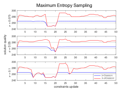
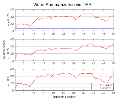
Figure 1: The solution quality achieved by the $\lambda$-Greedy after each constraints’ update, using a restart strategy, and the $\lambda$-dGreedy operator. Each plot shows results for a fixed standard deviation choice [$\sigma$] and fixed update frequency $\tau=30K$ (for the Maximum Entropy Sampling) and $\tau=50K$ (for Video Summarization).

We consider the problem of maximizing the entropy $f$ under a partition matroid constraint. This additional side constraint requires an upper bound on the number of sensors that can be chosen in given geographical areas. Specifically, we partition the total number of time series in seven sets, based on the continent in which the corresponding stations are located. Under this partition set, we then have seven independent cardinality constraints, one for each continent.
We use the Berkeley Earth Surface Temperature Study, which combines $1.6$ billion temperature reports from $16$ preexisting data archives. This archive contains over $39000$ unique stations from around the world. More information on the Berkeley Earth project can be found in [2]. Here, we consider unique time series defined as the average monthly temperature for each station. Taking into account all data between years $2015$-$2017$, we obtain $2736$ time series from the corresponding stations. Our experimental framework follows along the lines of [15].

In our dynamic setting, for each continent, a given parameter $d_{i}$ is defined as a percentage value of the overall number of stations available on that continent, for all $i\in[7]$. We let parameters $d_{1},\dots,d_{7}$ vary over time, as to simulate a setting where they are updated dynamically. This situation could occur when operational costs slightly vary overtime. We initially set all parameters to use $50\%$ of the available resources, and we introduce a variation of these parameters at regular intervals, according to $\mathcal{N}(0,\sigma^{2})$, a Gaussian distribution of mean $0$ and variance $\sigma^{2}$, for all $i\in[7]$.
We consider various choices for the standard deviation $\sigma$, and various choices for the time span between one dynamic update and the next one (the parameter $\tau$). For each choice of $\sigma$ and $\tau$, we consider a total of $50$ sequences of changes. We perform statistical validation using the Kruskal-Wallis test with $95$% confidence. In order to compare the results, we use the Bonferroni post-hoc statistical procedure. This method is used for multiple comparisons of a control algorithm against two or more other algorithms. We refer the reader to [9] for more detailed descriptions of these statistical tests.

We compare the results in terms of the solution quality achieved at each dynamic update by the $\lambda$-Greedy and the $\lambda$-dGreedy. We summarize our results in the Table LABEL:tbl:greedy_matroid (left) as follows. The columns correspond to the results for $\lambda$-Greedy and the $\lambda$-dGreedy respectively, along with the mean value, standard deviation, and statistical comparison. The symbol $X^{(+)}$ is equivalent to the statement that the algorithm labelled as $X$ significantly outperformed the other one.
Table LABEL:tbl:greedy_matroid (left) shows that the $\lambda$-dGreedy has a better performance than the $\lambda$-Greedy algorithm with restarts, when dynamic changes occur, especially for the highest frequencies $\tau=10K,20K$. This shows that the $\lambda$-dGreedy is suitable in settings when frequent dynamic changes occur. The $\lambda$-Greedy yields improved performance with lower frequencies, but it under-perform the $\lambda$-dGreedy on our dataset.
Figure 1 (left) shows the solution quality values achieved by the $\lambda$-Greedy and the $\lambda$-dGreedy, for different choices of the standard deviation $\sigma=0.075,0.05,0.1$. Again, we observe that the $\lambda$-dGreedy finds solutions that have better quality than the $\lambda$-Greedy with restarts. Even though the $\lambda$-dGreedy in some cases aligns with the $\lambda$-Greedy with restarts, the performance of the $\lambda$-dGreedy is clearly better than that of the simple $\lambda$-Greedy with restarts. The code for this set of experiments is available upon request.

Determinantal Point Processes

We conclude with a dynamic set of experiments on a video summarization task as in Section 5. We define the corresponding matrix $L$ using the quality-diversity decomposition, as proposed in [20]. Specifically, we define the coefficients $L_{i,j}$ of this matrix as $L_{i,j}=q(i)k(i,j)q(j)$, with $q(i)$ representing the quality of the $i$-th frame and $k(i,j)$ being the diversity between the $i$-th and $j$-th frame.
For the diversity measure $k$, we consider commonly used features $f\in F$ for pictures, and we use these features to define corresponding feature vectors $v^{f}_{i}$ for each frame $i$. Then the diversity measure is defined as

$$k(i,j)=\exp\left(-\sum_{f\in F}\frac{||v^{f}_{i}-v^{f}_{j}||_{2}^{2}}{\sigma_{f}}\right),$$

with $\sigma_{f}$ a parameter for this feature. To learn these parameters we use the Markov Chain Monte Carlo (MCMC) method (see [1]).

We use movie clips from the Frames Labeled In Cinema dataset [14]. We use 16 movies with 150-550 frames each to learn the parameters and one test movie with approximately 400 frames for our experiments. For each movie, we generate 5-10 samples (depending on the total amount of frames) of sets with 10-20 frames as training data. We then use MCMC on the training data to learn the parameters for each movie. When testing the $\lambda$-Greedy and the $\lambda$-dGreedy, we use the sample median of the trained parameters.

In this set of experiments, we consider a constraint by which the set of selected frames must not exceed a memory threshold. We define a cost function $c(S)$ as the sum of the size of each frame in $S$. As each frame comes with its own size in memory, choosing the best frames under certain memory budget is equivalent to maximizing a submodular function under a linear knapsack constraint.
The weight $W$ is given range $[0\%,100\%]$, with respect to the total weight $c(V)$, and it is updated dynamically throughout the optimization process, according to a Gaussian distribution $\mathcal{N}(0,\sigma^{2})$, for a given variance $\sigma^{2}$. This settings simulates a situation by which the overall available memory exhibits small frequent variation.

We select various parameter choices for the standard deviation $\sigma$, and the frequency $\tau$ with which a dynamic update occurs. We investigate the settings $\sigma$ = $0.075$, $0.05$, $0.1$, and $\tau$ = $10K$, $20K$, $30K$, $40K$, $50K$. Each combination of $\sigma$ and $\tau$ carries out $50$ dynamic changes. Again, we validate our results using the Kruskal-Wallis test with $95$% confidence. To compare the obtained results, we apply the Bonferroni post-hoc statistical test [9].

The results are presented in the Table LABEL:tbl:greedy_knapsack (right). We observe that the $\lambda$-dGreedy yields better performance than the $\lambda$-Greedy with restarts when dynamic changes occur. Similar findings are obtained when comparing a different standard deviation choice $\sigma$ = $0.075$, $0.05$, $0.1$. Specifically, for the highest frequency $\tau=10K$, the $\lambda$-dGreedy achieves better results by approximately one order of magnitude.
Figure 1 (right) shows the solution quality values obtained by the $\lambda$-dGreedy and the $\lambda$-Greedy, as the frequency is set to $\tau=50K$. It can be observed that, for $\sigma$ = $0.075$, $0.05$, $0.1$, the $\lambda$-dGreedy significantly outperforms the $\lambda$-Greedy with restarts, for almost all $50$ updates. The code for this set of experiments is available upon request.

8 CONCLUSION

Many real-world optimization problems can be approached as submodular maximization with multiple knapsack constraints (see Problem 2). Previous studies for this problem show that it is possible to approach this problem with a variety of heuristics. These heuristics often involve a local search, and require continuous relaxations of the discrete problem, and they are impractical. We propose a simple discrete greedy algorithm (see Algorithm 1) to approach this problem, that has polynomial run time and yields strong approximation guarantees for functions with bounded curvature (see Definition 2 and Theorem 4.1).

Furthermore, we study the problem of maximizing a submodular function, when knapsack constraints involve dynamic components. We study a setting by which the weights $W_{i}$ of a given set of knapsack constraints change overtime. To this end, we introduce a robust variation of our $\lambda$-Greedy algorithm that allows for handling dynamic constraints online (see Algorithm 2). We prove that this operator allows to maintain strong approximation guarantees for functions with bounded curvature, when constraints change dynamically (see Theorem 4.2).

We show that, in static settings, Algorithm 1 competes with Fantom, which is a popular algorithm for handling these constraints (see Table 1). Furthermore, we show that the $\lambda$-dGreedy is useful in dynamic settings. To this end, we compare the $\lambda$-dGreedy with the $\lambda$-Greedy combined with a restart policy, by which the optimization process starts from scratch at each dynamic update. We observe that the $\lambda$-dGreedy yields significant improvement over a restart in dynamic settings with limited computational time budget (see Figure 1 and Table LABEL:tbl:greedy_matroid).

Appendix: Missing Proofs

Proof of Theorem 4.1

We first observe that, for a given $\lambda$, the $\lambda$-Greedy has two phases. During the first phase, $\lambda$-Greedy adds points to the current solution iteratively. During the second phase, $\lambda$-Greedy finds the optimum among single-element sets and sets containing only elements whose cost is lower-bounded with $c_{i}(e)>\lambda W_{i}/\lambda$ for all $i\in[n]$. The greedy procedure requires at most $\mathcal{O}\left(n^{2}\right)$ steps, while the second procedure requires at most $\mathcal{O}\left(n^{k/\lambda}\right)$ steps, since all feasible solutions such that $c_{i}(e)>\lambda W_{i}/k$ consist of at most $k/\lambda$ points. Hence, the resulting run time is $\mathcal{O}\left(n^{\max(k/\lambda,2)}\right)$ run time.

We now prove the $\lambda$-Greedy yields the desired approximation guarantee. To this end, we define

$$\mathcal{V}=V_{1}=\{e\in V\colon c_{j}(e)\leq\lambda W_{j}/k\ \forall j\in[k]\}\quad\mbox{and}\quad V_{2}=V\setminus V_{1}.$$

Without loss of generality we assume that $W_{1}=\dots=W_{k}$. We denote with $W$ the weight of each knapsack. Let $\sigma_{t}$ be a solution of the greedy phase at time step $t$. Let $r\geq 0$ be the smallest index, such that

1. $c_{j}(\sigma_{t})\leq W$ for all $j\in[k]$, for all $t\in[r-1]$;

2. there exists $j\in[k]$ such that $c_{j}(\sigma_{r})>W$.

In other words, $r$ is the first point it time such that the new greedy solution does not fulfill all knapsacks at the same time. We first prove that either the solution $\sigma_{r-1}$ or the point $v^{*}=\operatorname*{arg\,max}_{e\in V}f(e)$ yields a good approximation guarantee of $\textsc{opt}\cap V_{1}$.

To simplify the notation, we define $f_{t}=f(\sigma_{t})-f(\sigma_{t-1})$ and $v_{t}=\sigma_{t}\setminus\sigma_{t-1}$, for all $t\in[r]$. We have that it holds

$$f_{\sigma_{t-1}}(\textsc{opt}\cap V_{1}) \leq\sum_{e\in\textsc{opt}\setminus\sigma_{t-1}}f_{\sigma_{t-1}}(e)$$ (1)

$$=\sum_{e\in(\textsc{opt}\cap V_{1})\setminus\sigma_{t-1}}\max_{j}c_{j}(e)\frac{f_{\sigma_{t-1}}(e)}{\max_{j}c_{j}(e)}$$ (2)

$$\leq\frac{f_{t}}{\max_{j}c(v_{t})}\sum_{e\in\textsc{opt}\setminus\sigma_{t-1}}\max_{j}c_{j}(e)$$ (3)

$$\leq\frac{\lambda W}{\max_{j}c(v_{i})}f_{t}$$ (4)

where (1) follows from the assumption that $f$ is submodular; (3) follows from (2) due to the greedy choice of Algorithm 1; (4) uses the fact that $c(\textsc{opt})\leq W$, together with the fact that $c(e)\leq W\lambda/k$ for all $c\in V_{1}$, for all $j\in[k]$. Rearranging yields

$$f_{t}\geq\frac{\max_{j}c_{j}(v_{i})}{\lambda W}(f(\sigma_{t-1}\cup(\textsc{opt}\cap V_{1}))-f(\sigma_{t-1})).$$ (5)

To continue with the proof, we consider the following lemma, which follows along the lines of Lemma 1 in [15].

Lemma 8.1.

Following the notation introduced above, define the set $J=\{t\in[n]\colon v_{t}\in\textsc{opt}\}$. Then for any subset $T\subseteq V$ it holds

$$f(\sigma_{t}\cup T)\geq f(T)+(1-\alpha)f(\sigma_{t})-(1-\alpha)\sum_{j\in[t]\cap J}f_{j}.$$

for all $t\in[r]$.

Proof 8.2.

From the definition of curvature we have that

$$f(\sigma_{i}\cup\textsc{opt})-f(\sigma_{i-1}\cup\textsc{opt})\geq(1-\alpha)\left(f(\sigma_{i})-f(\sigma_{i-1})\right).$$

for all $i=1,\dots,t$. It follows that

$$f(\sigma_{t}\cup\textsc{opt}) \geq f(\sigma_{t-1}\cup\textsc{opt})+(1-\alpha)\left(f(\sigma_{t})-f(\sigma_{t-1})\right)$$ (6)

$$\geq f(\emptyset\cup\textsc{opt})+\sum_{j=1}^{t}(1-\alpha)\left(f(\sigma_{j})-f(\sigma_{j-1})\right)$$ (7)

$$=f(\textsc{opt})+(1-\alpha)\left(f(\sigma_{t})-f(\emptyset)\right),$$ (8)

where (7) follows by iteratively applying (6) to the $f(U_{j-1}\cup\textsc{opt})$, and (8) follows by taking the telescopic sum.

Note that Lemma 8.1 yields $f(\sigma_{t}\cup(\textsc{opt}\cap V_{1}))\geq f(\textsc{opt}\cap V_{1})+(1-\max(1,\alpha))f(\sigma_{t})$, since $\alpha\in[0,1]$ if and only if the function $f$ is monotone. Combining this observation with (5) yields

$$f_{t} \geq\frac{\max_{j}c_{j}(v_{i})}{{\max(1,\alpha)}\lambda W}f(\textsc{opt}\cap V_{1})-\frac{\max_{j}c_{j}(v_{i})}{\lambda W}\sum_{i\in[t-1]}f_{i},$$

where we have simply used the telescopic sum over the $f(\sigma_{t})$. Defining $x_{t}=f_{t}/f(\textsc{opt}\cap V_{1})$ for all $t\in[r]$ we can write the inequality above as

$$\frac{{\max(1,\alpha)}\lambda W}{\max_{j}c_{j}(v_{t})}x_{t}+\max(1,\alpha)\sum_{i\in[t-1]}x_{i}\geq 1.$$ (9)

We conclude the proof by showing that any array of solutions $(x_{1},\dots,x_{n})$ with coefficients $x_{i}\in[0,1]$ that fulfils the LP as in (9) yields

$$\sum_{t\in[r]}x_{t}\geq\sum_{t\in[r]}\frac{\max_{j}c_{j}(v_{t})}{{\max(1,\alpha)}\lambda W}\prod_{i\in[t-1]}\left(1-\frac{\max_{j}c_{j}(v_{i})}{\lambda W}\right).$$ (10)

In order to prove (10), since it holds $x_{t}\in[0,1]$ for all $t\in[r]$, we can simplify our setting, by studying the system

$$\frac{{\max(1,\alpha)}\lambda W}{\max_{j}c_{j}(v_{t})}x_{t}+\max(1,\alpha)\sum_{i\in[t-1]}x_{i}=1.$$ (11)

This is due to the fact that the sum of the coefficients of any solution of (11) are upper-bounded by the sum of the coefficients of a solution of (10). We continue with the following simple lemma.

Lemma 8.3.

Let $(x_{1},\dots,x_{r})$ be a solution of the LP as in (11). Than it holds

$$x_{t}\geq\frac{\max_{j}c_{j}(v_{t})}{{\max(1,\alpha)}\lambda W}\prod_{i\in[t-1]}\left(1-\frac{\max_{j}c_{j}(v_{i})}{\lambda W}\right),$$

for all $t\in[r]$.

Proof 8.4.

Define $c_{t}=\max_{j}c_{j}(v_{t})/({\max(1,\alpha)}\lambda W)$ for all $t\in[r]$. Then the LP as in (11) can be written as

$$\frac{x_{t}}{c_{t}}=1-\max(1,\alpha)\sum_{i=1}^{t-1}x_{t}.$$

By defining $y_{t}=x_{t}/c_{t}$ for all $t\in[r]$, we have that $y_{t}-y_{t-1}=-\max(1,\alpha)x_{t-1}=-\max(1,\alpha)c_{t-1}y_{t-1}$, and we obtain the following recurrent relation $y_{t}+(\max(1,\alpha)c_{t}-1)y_{t-1}=0$, for all $t>1$. This is a recurrent linear equation with solutions

$$y_{t}=\prod_{j=1}^{t-1}(1-\max(1,\alpha)c_{j}).$$

The claim follows, by substituting $x_{t}$ in the equation above.

Hence, we have that it holds

$$f(\sigma_{r}) =f(\textsc{opt}\cap V_{1})\sum_{t}x_{t}$$ (12)

$$\geq f(\textsc{opt}\cap V_{1})\sum_{t}\frac{\max_{j}c_{j}(v_{t})}{{\max(1,\alpha)}kW}\prod_{i\in[t-1]}\left(1-\frac{\max_{j}c_{j}(v_{i})}{\lambda W}\right)$$ (13)

$$\geq\frac{f(\textsc{opt}\cap V_{1})}{\max(1,\alpha)}\left(1-\prod_{i\in[r]}\left(1-\frac{\max_{j}c_{j}(v_{i})}{\lambda W}\right)\right)$$ (14)

$$\geq\frac{f(\textsc{opt}\cap V_{1})}{\max(1,\alpha)}\left(1-\exp\left\{-\sum_{i\in[r]}\frac{\max_{j}c_{j}(v_{i})}{\lambda W}\right\}\right),$$ (15)

where (12) holds by taking the telescopic sum; (13) follows from Lemma 8.3; (14) follows via standard calculations; (15) follows because $1-x\leq e^{-x}$. Consider an index $\ell$ such that $c_{\ell}(\sigma_{r})>W$. We have that it holds

$$f(\sigma_{r}) \geq\frac{1}{\max(1,\alpha)}\left(1-\exp\left\{-\max(1,\alpha)\sum_{i\in[r]}\frac{\max_{j}c_{j}(v_{i})}{\lambda W}\right\}\right)f(\textsc{opt}\cap V_{1})$$

$$\geq\frac{1}{\max(1,\alpha)}\left(1-\exp\left\{-\max(1,\alpha)\sum_{i\in[r]}\frac{c_{\ell}(v_{i})}{\lambda W}\right\}\right)f(\textsc{opt}\cap V_{1})$$

$$\geq\frac{1}{\max(1,\alpha)}\left(1-e^{-1/\lambda}\right)f(\textsc{opt}\cap V_{1}).$$

We conclude by proving that Algorithm 1 yields the the desired approximation guarantee. To this end, let

$$U=\operatorname*{arg\,max}_{\{W\subseteq V_{2}\colon c_{j}(U)\leq W_{j}\ \forall j\in[k]\}}\left\{f(W)\geq f(\textsc{opt}\cap V_{2})\right\}.$$

Hence, following the notation of Algorithm 1, and denoting with $v*$ the point with maximum $f$-value among the singletons, it follows that

$$\operatorname*{arg\,max}\{f(\sigma_{r-1}),f(U),f(v^{*})\} \geq\frac{1}{3}(f(\sigma_{r-1})+f(U)+f(v^{*}))$$

$$\geq\frac{1}{3}(f(\sigma_{r-1})+f(v_{r})+f(U))$$

$$\geq\frac{1}{3}f(\sigma_{r}+f(U))$$

$$\geq\frac{1}{3\max(1,\alpha)}\left(1-e^{-1/\lambda}\right)f(\textsc{opt}\cap V_{1})+f(\textsc{opt}\cap V_{2})$$

$$\geq\frac{1}{3\max(1,\alpha)}\left(1-e^{-1/\lambda}\right)f(\textsc{opt}),$$

where the last inequality follows from submodularity. The claim follows.

Proof of Theorem 4.2

We prove that the claim holds after $\ell>1$ weights updates were given since the beginning of the optimization process. We denote with $W_{i}^{*}=\{W_{i,1},\dots,W_{i,k}\}$ the $i$-th new sequence of dynamic weights. Furthermore, define $\chi_{\ell}=\min\{\left\lvert\chi(c,W_{\ell})\right\rvert,\left\lvert\chi(c,W_{\ell-1})\right\rvert\}$ and $\mathcal{V}_{\ell}=\{e\in V\colon c_{i}(e)\leq\lambda W_{\ell,i}/k\ \forall i\in[k]\}$., let $\sigma_{\ell,t}$ be as the current solution at time step $t$, after new dynamic weights $W_{\ell}^{*}$ were given. Let $r_{\ell}\geq 0$ be the smallest index, such that

1. $c_{i}(\sigma_{\ell,t})\leq W_{\ell,i}$, for all $e\in V$, $t\in[r_{\ell}-1]$ and for all $i\in[k]$;

2. $c_{i}(\sigma_{\ell,r_{\ell}})>W_{\ell,i}$, for some $i\in[k]$.

In other words, $r_{\ell}$ is the first point it time, after the ${\ell}$-th weight update, such that the set maximizing the greedy step is not feasible. We prove that the $\lambda$-dGreedy maintains the desired approximation guarantee. Note that at each step, the $\lambda$-dGreedy requires at most $n$ calls to the value oracle function. Then the $\lambda$-Greedy with restarts requires $\mathcal{O}\left(n(n-\chi_{\ell}))\right)$ additional run time to construct the solution $\sigma_{{\ell},r_{\ell}}$.

In order to prove the desired lower-bound on the approximation guarantee, we prove that the solution $\sigma_{\ell,r_{\ell}}$ is identical to a solution of the same size constructed by the $\lambda$-Greedy starting from the empty set, under side constraints specified by $W_{\ell}^{*}$. The claim then follows, by readily applying Theorem 4.1.

Define $d_{i}=\sigma_{\ell,r_{\ell}}$ and denote with $\{v_{{\ell},1},\dots,v_{{\ell},t},\dots,v_{{\ell},d_{\ell}}\}$ the points of $\sigma_{\ell,r_{\ell}}$ sorted in the order that they were added to the solution. Define the sets

$$\begin{array}[]{lcl}\hat{\sigma}_{{\ell},t}=\emptyset&\mbox{for }&t=0;\\ \hat{\sigma}_{{\ell},t}=\{v_{{\ell},1},\dots,v_{{\ell},t}\}&\mbox{for }&t\in[d_{\ell}];\\ \end{array}$$

Note that, according to this definition, it holds $\hat{\sigma}_{{\ell},t}=\sigma_{{\ell},r_{\ell}}$ for all ${\ell}\in[m]$. We prove that the solution $\sigma_{{\ell},r_{\ell}}$ is equal to a solution if the same size constructed by the $\lambda$-Greedy from scratch, by showing that it holds

$$v_{{\ell},t}=\operatorname*{arg\,max}_{e\in V\setminus\hat{\sigma}_{{\ell},t-1}}\frac{f_{\hat{\sigma}_{{\ell},t-1}}(e)}{\max_{j}c_{j}(e)}$$ (16)

for all $t\in[d_{\ell}]$, for all ${\ell}\in[m]$, with an induction argument on ${\ell}$. The base case for ${\ell}=1$ holds due to the greedy rule, since in this case the optimization process consists of greedily adding points to the current solution, starting from the empty set.

For the inductive case, suppose that the claim holds for all runs up to ${\ell}-1$. Note that, since the functions $c_{j}$ are linear, it holds

$$c_{j}(T)\leq\sum_{e\in T}\max_{j}c_{j}(e)\leq\sum_{e\in\chi_{\ell}}\max_{j}c_{j}(e)\leq W_{\ell,j},$$

for all $T\in V$ such that $\left\lvert T\right\rvert\leq\left\lvert\chi_{\ell}\right\rvert$. Hence, all subsets of $V$ of size at most $T$ are feasible solutions in the $k$-knapsack intersection. Similarly, one can prove that $c_{j}(T)\leq W_{\ell-1,j}$, for all $T\in V$ such that $\left\lvert T\right\rvert\leq\left\lvert\chi_{\ell}\right\rvert$. Hence, all solutions with size at most $\left\lvert\chi\right\rvert$ are feasible in both constraints defined by $W_{\ell-1}^{*}$ and $W_{\ell}^{*}$. In particular, solutions obtained by Algorithm 1 up to size at most $\left\lvert\chi_{\ell}\right\rvert$, are identical in both constraints, i.e. $\hat{\sigma}_{\ell,t}=\hat{\sigma}_{\ell-1,t}$. Combining these observations with the inductive hypothesis on $v_{{\ell}-1,t}$, we get

$$v_{{\ell},t}=v_{{\ell}-1,t}=\operatorname*{arg\,max}_{e\in V\setminus\hat{\sigma}_{{\ell}-1,t-1}}\frac{{f}_{\hat{\sigma}_{{\ell}-1,t-1}}(e)}{\max_{j}c_{j}(e)}=\operatorname*{arg\,max}_{e\in V\setminus\hat{\sigma}_{i,t-1}}\frac{{f}_{\hat{\sigma}_{{\ell},t-1}}(e)}{\max_{j}c_{j}(e)},$$

for all $t\leq\left\lvert\chi_{\ell}\right\rvert$. We conclude that (16) holds for all $v_{i,t}$ with $t\leq\left\lvert\chi_{\ell}\right\rvert$. Note that for $\left\lvert\chi_{\ell}\right\rvert<t\leq r_{\ell}$ the claim holds due to the greedy rule, hence (16) holds. Furthermore, note that the new solution is in the set $\mathcal{V}_{\ell}$. Combining Theorem 4.1 with (16), we conclude that $\sigma_{\ell,r_{\ell}}$ yields the desired approximation guarantee.

References

- [1] Raja Hafiz Affandi, Emily B. Fox, Ryan P. Adams, and Benjamin Taskar, ‘Learning the parameters of determinantal point process kernels’, in Proc. of ICML, pp. 1224–1232, (2014).
- [2] Berkeley Earth. The berkeley earth surface temperature study. http://www.berkeleyearth.org, 2019.
- [3] Andrew An Bian, Joachim M. Buhmann, Andreas Krause, and Sebastian Tschiatschek, ‘Guarantees for greedy maximization of non-submodular functions with applications’, in Proc. of ICML, pp. 498–507, (2017).
- [4] Allan Borodin, Aadhar Jain, Hyun Chul Lee, and Yuli Ye, ‘Max-sum diversification, monotone submodular functions, and dynamic updates’, ACM Transactions on Algorithms, 13(3), 41:1–41:25, (July 2017).
- [5] Chandra Chekuri, Jan Vondrák, and Rico Zenklusen, ‘Submodular function maximization via the multilinear relaxation and contention resolution schemes’, SIAM Journal of Computing, 43(6), 1831–1879, (2014).
- [6] Raymond Chiong, Thomas Weise, and Zbigniew Michalewicz, Variants of evolutionary algorithms for real-world applications, Springer, 2012.
- [7] Jung Jin Cho, Yong Chen, and Yu Ding, ‘On the (co)girth of a connected matroid’, Discrete Applied Mathematics, 155(18), 2456–2470, (2007).
- [8] Michele Conforti and Gérard Cornuéjols, ‘Submodular set functions, matroids and the greedy algorithm: Tight worst-case bounds and some generalizations of the rado-edmonds theorem’, Discrete Applied Mathematics, 7(3), 251–274, (1984).
- [9] Gregory W. Corder and Dale I. Foreman, Nonparametric statistics for non-statisticians: a step-by-step approach, Wiley, 2009.
- [10] Abhimanyu Das and David Kempe, ‘Approximate submodularity and its applications: Subset selection, sparse approximation and dictionary selection’, Journal of Machine Learning Research, 19, 3:1–3:34, (2018).
- [11] Benjamin Doerr, Carola Doerr, Aneta Neumann, Frank Neumann, and Andrew M. Sutton, ‘Optimization of chance-constrained submodular functions’, in Proc. of AAAI, (2020). to appear.
- [12] Salman Fadaei, MohammadAmin Fazli, and MohammadAli Safari, ‘Maximizing non-monotone submodular set functions subject to different constraints: Combined algorithms’, Operations Research Letters, 39(6), 447 – 451, (2011).
- [13] Mahyar Fazlyab, Santiago Paternain, Victor M. Preciado, and Alejandro Ribeiro, ‘Interior point method for dynamic constrained optimization in continuous time’, in ACC, pp. 5612–5618. IEEE, (2016).
- [14] FLIC Dataset. Frames labeled in cinema. https://bensapp.github.io/flic-dataset.html, 2019.
- [15] Tobias Friedrich, Andreas Göbel, Frank Neumann, Francesco Quinzan, and Ralf Rothenberger, ‘Greedy maximization of functions with bounded curvature under partition matroid constraints’, in Proc. of AAAI, pp. 2272–2279, (2019).
- [16] Boqing Gong, Wei-Lun Chao, Kristen Grauman, and Fei Sha, ‘Diverse sequential subset selection for supervised video summarization’, in Proc. of NIPS, pp. 2069–2077, (2014).
- [17] Sanjay Dominik Jena, Jean-François Cordeau, and Bernard Gendron, ‘Solving a dynamic facility location problem with partial closing and reopening’, Computers & Operations Research, 67(C), 143–154, (March 2016).
- [18] Samir Khuller, Anna Moss, and Joseph Naor, ‘The budgeted maximum coverage problem’, Information Processing Letters, 70(1), 39–45, (1999).
- [19] Andreas Krause, Ajit Paul Singh, and Carlos Guestrin, ‘Near-optimal sensor placements in gaussian processes: Theory, efficient algorithms and empirical studies’, Journal of Machine Learning Research, 9, 235–284, (2008).
- [20] Alex Kulesza and Ben Taskar, ‘Structured determinantal point processes’, in Proc. of NIPS, pp. 1171–1179, (2010).
- [21] Alex Kulesza and Ben Taskar, ‘Determinantal point processes for machine learning’, Foundations and Trends in Machine Learning, 5(2-3), 123–286, (2012).
- [22] Ariel Kulik, Hadas Shachnai, and Tami Tamir, ‘Approximations for monotone and nonmonotone submodular maximization with knapsack constraints’, Mathematics of Operations Research, 38(4), 729–739, (2013).
- [23] Jon Lee, Vahab S. Mirrokni, Viswanath Nagarajan, and Maxim Sviridenko, ‘Non-monotone submodular maximization under matroid and knapsack constraints’, in Proc. of STOC, pp. 323–332, (2009).
- [24] Hui Lin and Jeff Bilmes, ‘Multi-document summarization via budgeted maximization of submodular functions’, in Proc. of NAACL-HLT, pp. 912–920, (2010).
- [25] Odile Macchi, ‘The coincidence approach to stochastic point processes’, Advances in Applied Probability, 7(1), 83–122, (1975).
- [26] Baharan Mirzasoleiman, Ashwinkumar Badanidiyuru, and Amin Karbasi, ‘Fast constrained submodular maximization: Personalized data summarization’, in Proc. of ICML, pp. 1358–1367, (2016).
- [27] Baharan Mirzasoleiman, Ashwinkumar Badanidiyuru, and Amin Karbasi, ‘Fast constrained submodular maximization: Personalized data summarization’, in Proc. of ICML, pp. 1358–1367, (2016).
- [28] Baharan Mirzasoleiman, Stefanie Jegelka, and Andreas Krause, ‘Streaming non-monotone submodular maximization: Personalized video summarization on the fly’, in Proc. of AAAI, pp. 1379–1386, (2018).
- [29] George L. Nemhauser, Laurence A. Wolsey, and Marshall L. Fisher, ‘An analysis of approximations for maximizing submodular set functions - I’, Mathematical Programming, 14(1), 265–294, (1978).
- [30] Vahid Roostapour, Aneta Neumann, and Frank Neumann, ‘On the performance of baseline evolutionary algorithms on the dynamic knapsack problem’, in Proc of. PPSN, pp. 158–169, (2018).
- [31] Vahid Roostapour, Aneta Neumann, Frank Neumann, and Tobias Friedrich, ‘Pareto optimization for subset selection with dynamic cost constraints’, in Proc. of AAAI, pp. 2354–2361, (2019).
- [32] Maxim Sviridenko, ‘A note on maximizing a submodular set function subject to a knapsack constraint’, Operation Research Letters, 32(1), 41–43, (2004).
- [33] Maxim Sviridenko, Jan Vondrák, and Justin Ward, ‘Optimal approximation for submodular and supermodular optimization with bounded curvature’, Mathematics of Operations Research, 42(4), (2017).
- [34] A. Vardy, ‘The intractability of computing the minimum distance of a code’, IEEE Transactions on Information Theory, 43(6), 1757–1766, (1997).
- [35] Qilian Yu, Easton Li Xu, and Shuguang Cui, ‘Streaming algorithms for news and scientific literature recommendation: Monotone submodular maximization with a d -knapsack constraint’, IEEE Access, 6, 53736–53747, (2018).
- [36] Haifeng Zhang and Yevgeniy Vorobeychik, ‘Submodular optimization with routing constraints’, in Proc. of AAAI, eds., Dale Schuurmans and Michael P. Wellman, pp. 819–826, (2016).
- [37] Jinging Zheng, Zhuolin Jiang, Rama Chellappa, and P. Jonathon Phillips, ‘Submodular attribute selection for action recognition in video’, in Proc. of NIPS, pp. 1341–1349, (2014).