Exact non-adiabatic part of the Kohn-Sham potential and its fluidic approximation

Abstract

We present a simple geometrical “fluidic” approximation to the non-adiabatic part of the Kohn-Sham potential, $v_{\mathrm{KS}}$, of time-dependent density functional theory. This part of $v_{\mathrm{KS}}$ is often crucial, but most practical functionals utilize an adiabatic approach based on ground-state DFT, limiting their accuracy in many situations. For a variety of model systems, we calculate the exact time-dependent electron density, and find that the fluidic approximation corrects a large part of the error arising from the “exact adiabatic” approach, even when the system is evolving far from adiabatically.

Time-dependent Kohn-Sham density functional theory Runge and Gross (1984); van Leeuwen (1999); Kohn and Sham (1965) (TDDFT) is in principle an exact and efficient theory of the dynamics of systems of interacting electrons. In practical applications, while performing well in some cases, its validity is often restricted by the limitations of available approximate functionals for electron exchange and correlation (xc). Typically, an adiabatic approximation to the xc potential is used, in which the instantaneous electron density is implicitly assumed to be in its ground state, thereby neglecting all “memory effects”. While these ground-state approximations have steadily improved Kohn and Sham (1965); Perdew and Zunger (1981); Perdew and Wang (1992); Perdew (1985); Burke et al. (1997); Perdew et al. (1992, 1996a, 1996b); Proynov et al. (1997); Van Voorhis and Scuseria (1998); Perdew et al. (1999); Sun et al. (2015), by definition they cannot approach the exact TDDFT potential: it is necessary to address the non-adiabatic contributions in order for TDDFT to be capable of predictive accuracy in relation to a multitude of applications to diverse fields such as the determination of electronic excitation energies including those of a charge-transfer nature Maitra (2017), electron dynamics Elliott et al. (2012) including non-perturbative charge transfer dynamics Fuks (2016), time-resolved spectroscopy Fuks et al. (2015) and electron scattering Suzuki et al. (2017).

In this paper, in order to clearly distinguish between adiabatic and non-adiabatic contributions, we consider the purest application of the concept of the adiabatic functional to the complete Kohn-Sham (KS) potential, $v_{\mathrm{KS}}$: at each instant, the DFT KS potential whose ground-state density is equal to the exact time-dependent density. The remainder of the exact $v_{\mathrm{KS}}$ constitutes the unambiguously non-adiabatic part, to which we also propose an approximation.

We work in the Runge-Gross formalism Runge and Gross (1984) of TDDFT, in which the exact xc potential, $v_{\mathrm{xc}}$, at time $t$ depends on the density at all points in space and all non-future times. It has been argued Dobson (1994); Vignale (1995a, b); Vignale and Kohn (1996) that the exact non-adiabatic functional often requires strong nonlocal temporal and spatial dependence on the density. A number of properties of the exact functional, such as the harmonic potential theorem (HPT) Dobson (1994) and zero-force theorem (ZFT) Vignale (1995a), have been used to identify limitations of previous approximate TDDFT functionals. Adiabatic functionals trivially satisfy many of these exact conditions through their complete lack of memory-dependence, yet prove inadequate in many applications Jamorski et al. (1996); Hessler et al. (2002); Dreuw et al. (2003); Maitra et al. (2004); Neugebauer et al. (2004); Cave et al. (2004); Ullrich and Tokatly (2006); Giesbertz et al. (2008); Fuks et al. (2011); Maitra (2016); Fuks (2016); Maitra (2017); Singh et al. (2019); Elliott et al. (2012); Fuks et al. (2015); Suzuki et al. (2017). The development of non-adiabatic functionals that continue to satisfy these exact properties is non-trivial. For example, it was shown that modifying the adiabatic local density approximation (ALDA) by introducing time-nonlocality, such as in the Gross-Kohn Gross and Kohn (1985) (GK) approximation, is inappropriate Vignale (1995a); Dobson (1994).

The best-known approximate non-adiabatic functional is that developed by Vignale and Kohn Vignale and Kohn (1996); Dobson et al. (2013); Vignale et al. (1997) (VK). This was constructed by studying the responses to slowly-varying perturbations of the homogeneous electron gas, and they found a time-dependent xc vector potential as a functional of the local current and charge densities $j$ and $n$, thereby implicitly obtaining a scalar potential which depends nonlocally on the density. While the VK formalism has proved promising van Faassen et al. (2002, 2003); de Boeij et al. (2001); Ullrich and Vignale (1998, 2001, 2002); Berger et al. (2006); D’Agosta and Vignale (2006); Nazarov et al. (2007); D’Amico and Ullrich (2006); Sai et al. (2005), not least through it obeying the HPT and ZFT, its validity is limited Berger et al. (2007); van Faassen and de Boeij (2004a, b); Ullrich and Burke (2004); Berger et al. (2005) owing to the constraints under which it was derived.

Our calculations employ the iDEA code Hodgson et al. (2013) which solves the many-electron Schrödinger equation exactly for small, one-dimensional prototype systems of spinless electrons . This gives us access to the exact electron density $n(x,t)$. We then determine the exact $v_{\mathrm{KS}}(x,t)$ through reverse engineering Ramsden and Godby (2012). We also obtain the exact adiabatic KS potential Hessler et al. (2002); Thiele et al. (2008); Maitra (2016) $v_{\mathrm{KS}}^{\mathrm{A}}$ by applying ground-state reverse engineering to the instantaneous density at each time . The exact non-adiabatic component $\Delta v_{\mathrm{KS}}$ is then $v_{\mathrm{KS}}-v_{\mathrm{KS}}^{\mathrm{A}}$.

In developing an approximation to $\Delta v_{\mathrm{KS}}$, it is helpful to consider the situation in different inertial frames, related through a Galilean transformation, as noted by Tokatly et al. Tokatly (2005a, b); Ullrich and Tokatly (2006); Tokatly (2006); Ullrich (2012). While $v_{\mathrm{KS}}^{\mathrm{A}}$ requires zero correction in any inertial frame when the density is fully static in one of these frames, in the more general case the non-adiabatic corrections to $v_{\mathrm{KS}}^{\mathrm{A}}$ may be expected to be at their smallest in the local, instantaneous rest frame of the density, defined by a transformation velocity of the local velocity field $u(x,t)=j(x,t)/n(x,t)$. In particular, the effects of acceleration ($\dot{u}\neq 0$) and dispersion ($\partial_{x}u\neq 0$) have least effect in a frame where $u$ itself is zero . Conveniently, introducing a vector potential $A=-u(x,t)$ in the original frame of reference is (apart from an unimportant temporal phase factor) equivalent to a Galilean transformation to the local instantaneous rest frame Tokatly (2005a, b). As described above, the non-adiabatic correction should be minimal in the latter frame, and here we adopt the simple assumption that it is zero. We term this the fluidic approximation. The resulting non-adiabatic correction in the original frame is therefore

$$\Delta v_{\mathrm{KS}}(x,t>0)=-\int_{-\infty}^{x}\frac{\partial}{\partial t}u(x^{\prime},t>0)\ dx^{\prime},$$ (1)

where we have gauge-transformed $A$ into a scalar potential. It is evident that the density-dependence of this $\Delta v_{\mathrm{KS}}$ is nonlocal in both space and time Vignale and Kohn (1996).

System 1 — As a first test of the fluidic approximation, we consider two interacting electrons in a potential well, which takes the form of an inverted Gaussian function. Initially in the ground state, a uniform electric field, $-\varepsilon x$, is applied at $t=0$, driving the electrons to the right and inducing a current [Fig. 1(a)]. The sudden application of the perturbation means that we are well outside of the adiabatic limit, and this can be seen by solving the time-dependent KS equations with the exact adiabatic KS potential, $v_{\mathrm{KS}}(t)=v_{\mathrm{KS}}^{\mathrm{A}}(t)$. By plotting the change in the electron density from the ground state, $\delta n$, we find $v_{\mathrm{KS}}^{\mathrm{A}}(t)$ on its own to be wholly inadequate ($\approx 13\%$ error in $n$ at $t=8$ a.u.), while adding the fluidic approximation substantially reduces this error to less than $1\%$ [Fig. 1(b)].

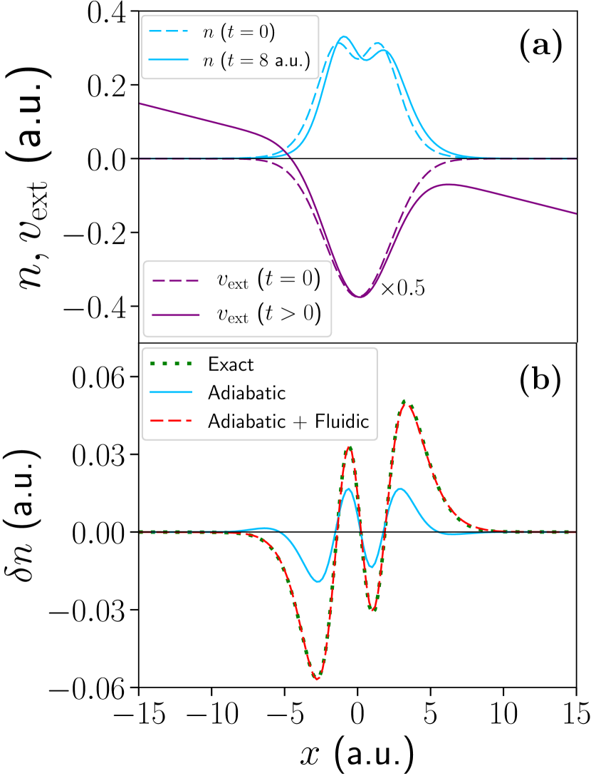
Figure 1: System 1: two interacting electrons in a Gaussian potential well, with a uniform electric field applied at $t=0$, driving the electrons to the right and inducing a current. (a) The ground-state external potential (dashed purple) and exact ground-state electron density (dashed blue), along with the perturbed external potential (solid purple) and exact time-dependent electron density at $t=8$ a.u. (solid blue). (b) The change in the exact electron density ($\delta n(x,t)=n(x,t)-n(x,0)$) at $t=8$ a.u. (short-dashed green), along with that obtained when using the exact $v_{\mathrm{KS}}^{\mathrm{A}}$ (solid blue), and when adding the exact $v_{\mathrm{KS}}^{\mathrm{A}}$ with the fluidic approximation $\Delta A_{\mathrm{KS}}=-u$ (dashed red). The exact adiabatic potential is clearly inadequate, but its error is substantially reduced by the fluidic approximation.

To understand these results we analyze the non-adiabatic correction to the KS potential in both its scalar and its vector forms. We find very good agreement between the exact $\Delta A_{\mathrm{KS}}$ and that obtained using the fluidic approximation $-u(x,t)$ [Fig. 2(a)]. The velocity field $u$ (the negative of the fluidic curve in Fig. 2(a)) quickly becomes strongly non-uniform in both space and time as the electrons explore excited states – far removed from a universal rest frame. Similarly close agreement between the exact and fluidic $\Delta v_{\mathrm{KS}}$ [Fig. 2(b)] is evident when the non-adiabatic correction is cast into its scalar form through Eq. (1).

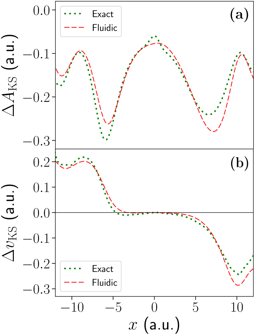
Figure 2: The non-adiabatic correction to the KS potentials for System 1. (a) The exact $\Delta A_{\mathrm{KS}}$ (short-dashed green) and that obtained using the fluidic approximation $\Delta A_{\mathrm{KS}}=-u$ (dashed red), at $t=8$ a.u. (b) The corresponding exact (short-dashed green) and fluidic (dashed red) $\Delta v_{\mathrm{KS}}$ in its scalar form. The fluidic approximation performs very well, even though the velocity field is non-uniform in both space and time. (The exact adiabatic approximation, of course, amounts to setting $\Delta A_{\mathrm{KS}}=\Delta v_{\mathrm{KS}}=0$.)

Systems 2A, 2B, 2C — We now consider a set of systems of interacting electrons in atomiclike external potentials which decay much more slowly at large $x$, $v_{\mathrm{ext}}=-a/(|x|+a)$ with $a=20$, thereby increasing correlation. At time $t=0$, a static sinusoidal perturbation of the form $\varepsilon\cos(0.75x)$ is applied, where $\varepsilon$ is 0.02 for System 2A (two electrons), 0.02 for System 2B (three electrons) and 0.1 for System 2C (three electrons).

In System 2A the sudden perturbation at $t=0$ acts to push the two electrons apart. This results in a velocity field that is varying in both space and time, as in System 1; in this case even the sign of $u$ is not the same for all $x$, which takes us even further away from a universal rest frame. Correspondingly, we find the exact adiabatic potential to be insufficient ($\approx 5\%$ error in $n$ at $t=5$ a.u.), while adding the fluidic approximation reduces this error to $\approx 1\%$. System 2B contains three interacting electrons in the same $v_{\mathrm{ext}}$ as System 2A. The additional electron results in a ground-state density that is much less spatially uniform. We run the simulation for 5 a.u. of time and find similar results: $v_{\mathrm{KS}}^{\mathrm{A}}$ produces an error in $n$ of $\approx 5\%$, and the fluidic approximation reduces this to $\approx 1\%$.

As mentioned above, the fluidic approximation assumes that a system remains close to its ground state in the local instantaneous rest frame. In order to stretch this approximation severely, in System 2C the perturbing potential is much stronger, resulting in a much larger response of the density [Fig. 3(a)]. The fluidic approximation still succeeds in reducing the error in the density, from $\approx 25\%$ where only the exact adiabatic potential is used, to $\approx 6\%$, at $t=5$ a.u. [Fig. 3(b)]. At later times, the dynamic (time-dependent) xc effects become very significant. To confirm this, we replace the xc component of the exact time-dependent $v_{\mathrm{KS}}$ with the fixed ground-state $v_{\mathrm{xc}}$, thereby suppressing the dynamic part, and find this potential to be wholly inadequate ($\approx 62\%$ error in $n$ at $t=18$ a.u.). Here, the exact adiabatic KS potential is better ($\approx 17\%$ error), while adding the fluidic approximation improves it further ($\approx 15\%$ error) [Fig. 3(c)].

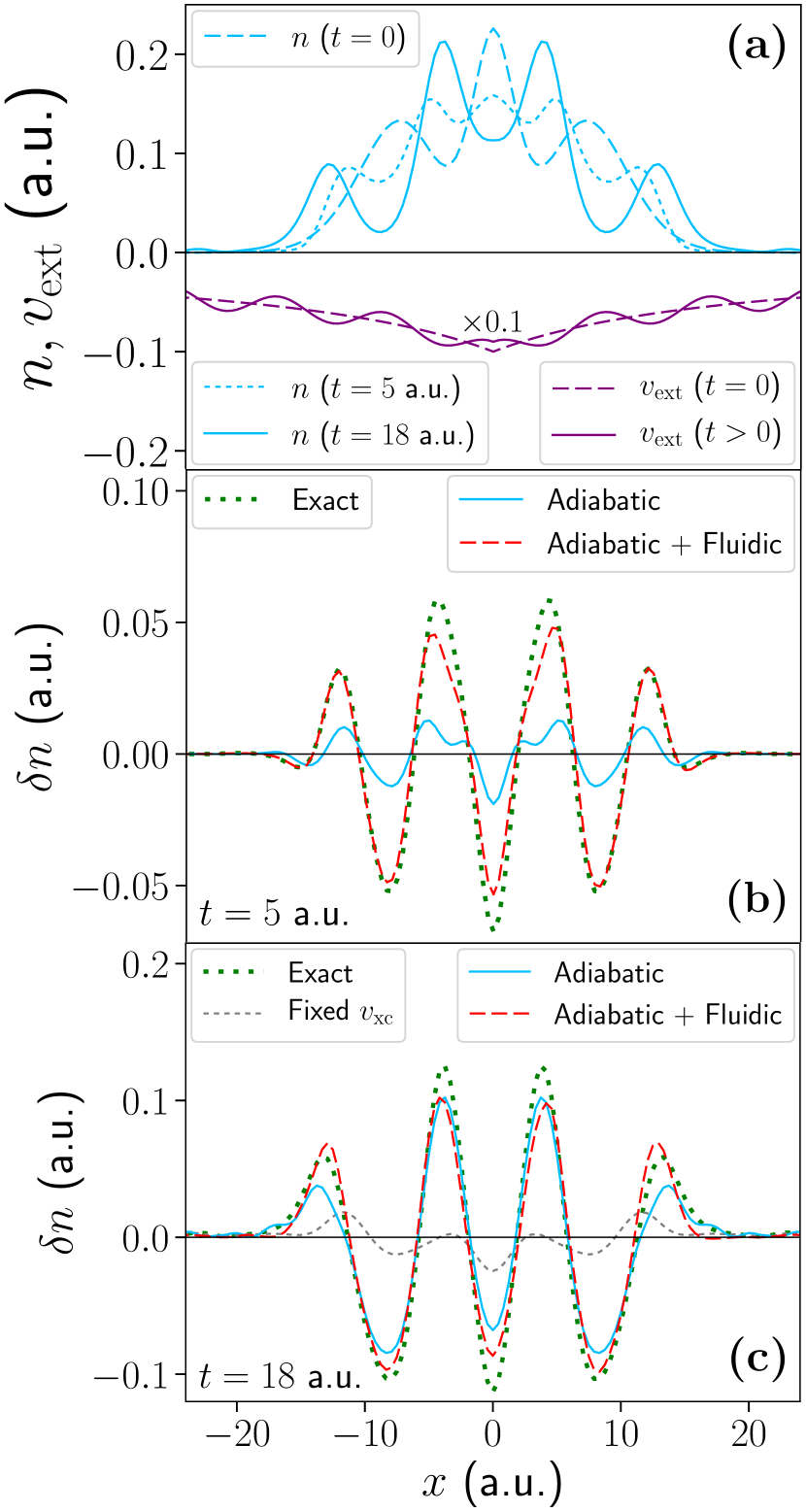
Figure 3: System 2C: three interacting electrons in an atomiclike potential, with a static sinusoidal perturbation applied at $t=0$, pushing the electrons apart. (a) The ground-state external potential (dashed purple) and exact ground-state electron density (dashed blue), along with the perturbed external potential (solid purple) and exact time-dependent electron density at $t=5$ a.u. (short-dashed blue) and $t=18$ a.u. (solid blue). (b) The change in the exact electron density at $t=5$ a.u. (short-dashed green), along with that obtained when using the exact $v_{\mathrm{KS}}^{\mathrm{A}}$ (solid blue), and when adding the exact $v_{\mathrm{KS}}^{\mathrm{A}}$ with the fluidic approximation (dashed red). Even though the density is strongly disrupted, the fluidic approximation remains successful. (c) The same as (b) but at $t=18$ a.u. where the dynamic xc contribution is very significant, evident by the completely inadequate result obtained with the fixed $v_{\mathrm{xc}}$ (short-dashed gray) (see main text). Here, the exact $v_{\mathrm{KS}}^{\mathrm{A}}$ is better, but adding the fluidic approximation improves it further.

Exact conditions — A number of properties of the exact xc functional are known, and these are often used to identify the limitations of approximate functionals. We now explore whether the fluidic approximation satisfies these exact conditions.

We begin with the one-electron limit, where the exact xc functional, when applied to a one-electron system, reduces to the negative of the Hartree potential $v_{\mathrm{H}}$, thereby canceling the spurious self-interaction. This means that $v_{\mathrm{KS}}$ is described exactly by a known functional Hessler et al. (2002); Elliott et al. (2012); Maitra (2016), which has been termed Hodgson et al. (2014) the single orbital approximation – itself capable of capturing features such as steps in the KS potential Elliott et al. (2012); Hodgson (2016) – whose non-adiabatic part is

$$\Delta v_{\mathrm{KS}}(x,t)=-\int_{-\infty}^{x}\frac{\partial}{\partial t}u(x^{\prime},t)\ dx^{\prime}-\frac{1}{2}u^{2}(x,t).$$ (2)

We note that the first term is the fluidic approximation [Eq. (1)]. We have studied systems of one electron in the external potentials from Systems 1, 2A and 2C, and confirm that the full Eq. (2) yields the exact $v_{\mathrm{KS}}$; here, the effect on the density of including the $-u^{2}/2$ term ranges from $<$0.1% (potential 2A) to 14% (potential 2C), so that the fluidic approximation alone is already satisfactory. Indeed, in our two- and three-electron systems, the effect of adding the additional term to the fluidic approximation is small and typically slightly deleterious.

The zero-force theorem Vignale (1995a) follows from Newton’s third law and requires the net force exerted on the system by $v_{\mathrm{H}}$ and $v_{\mathrm{xc}}$ to vanish. At the level of the KS potential, $\int n(x,t)\partial_{x}\Delta v_{\mathrm{KS}}(x,t)\ dx=\int n(x,t)\partial_{x}v_{\mathrm{ext}}(x,t)\ dx$, since the exact $v_{\mathrm{KS}}^{\mathrm{A}}$ satisfies the theorem in its own right. In the fluidic approximation for System 1 , the left and right hand sides of this equation are within 11 % of one another, so that the theorem appears to be approximately obeyed.

The harmonic potential theorem Dobson (1994) shows that in a system of interacting electrons in a harmonic potential, subject to a uniform electric field at $t=0$, the density rigidly moves in the manner of the underlying classical harmonic oscillator. We have shown that the fluidic approximation adds exactly the non-adiabatic correction required by the HPT. We have also confirmed this numerically for two interacting electrons in a harmonic potential.

A constraint that can be challenging for non-adiabatic functionals is the memory condition Maitra et al. (2002), which notes that $v_{\mathrm{xc}}(t)$ and hence $v_{\mathrm{KS}}(t)$ must be independent of which previous instant in the evolution of the system is to be used to designate the “initial state”. This is violated by the VK functional Maitra (2016). Eq. (1) demonstrates that the fluidic approximation satisfies this memory condition by virtue of its dependence only on the instantaneous rate of change of $u$, and not its full history.

System 3 — As a challenging test of the fluidic approximation, we finally consider two interacting electrons in a tunneling system. Initially $v_{\mathrm{ext}}$ is a symmetric double-well potential, with one electron localized in each well. At $t=0$, the left-hand well is raised and the right-hand well lowered, initiating tunneling through the barrier [Fig. 4]. A tunneling electron has an imaginary momentum, meaning that the (real) velocity field is of less physical significance. Correspondingly, the fluidic approximation recovers less of the adiabatic density error, but nevertheless reduces it from $\approx 8\%$ to $\approx 4\%$, at $t=15$ a.u. Accordingly, the tunneling rate from the left-hand side to the right-hand side is initially improved, but this is not the case at later times [inset of Fig. 4].

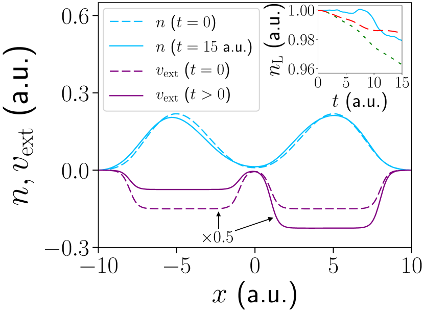
Figure 4: System 3: two interacting electrons in a tunneling system. Inset: The exact total electron number on the left-hand side ($x<0$) (short-dashed green); also the exact adiabatic (solid blue) and fluidic approximation (dashed red).

In summary, we have calculated the exact adiabatic and non-adiabatic parts of the KS potential, $v_{\mathrm{KS}}^{\mathrm{A}}$ and $\Delta v_{\mathrm{KS}}$, for a variety of model systems. $\Delta v_{\mathrm{KS}}$ is precisely defined by our procedure, and represents the part of the time-dependent KS potential that is intrinsically unobtainable from a ground-state functional. Our key finding is that a simple geometrical approximation to this non-adiabatic KS potential – making use of a Galilean transformation to the local instantaneous rest frame – recovers most of the density error attributable to the exact adiabatic approach: typically $80-95\%$ in the ballistic systems studied. Studies of additional systems should further illuminate this decomposition of the KS potential of TDDFT in highly non-adiabatic situations, with the fluidic approximation providing a solid foundation for a hierarchy of approximations to $\Delta v_{\mathrm{KS}}$.

We thank Jack Wetherell and Nick Woods for recent developments in the iDEA code, and Matt Hodgson and Carsten Ullrich for helpful comments. Data created during this research is available from the York Research Database .

References

- Runge and Gross (1984) E. Runge and E. K. U. Gross, Phys. Rev. Lett. 52, 997 (1984).
- van Leeuwen (1999) R. van Leeuwen, Phys. Rev. Lett. 82, 3863 (1999).
- Kohn and Sham (1965) W. Kohn and L. J. Sham, Phys. Rev. 140, A1133 (1965).
- Perdew and Zunger (1981) J. P. Perdew and A. Zunger, Phys. Rev. B 23, 5048 (1981).
- Perdew and Wang (1992) J. P. Perdew and Y. Wang, Phys. Rev. B 45, 13244 (1992).
- Perdew (1985) J. P. Perdew, Phys. Rev. Lett. 55, 1665 (1985).
- Burke et al. (1997) K. Burke, J. P. Perdew, and Y. Wang, Derivation of a generalized gradient approximation: The pw91 density functional, in Electronic Density Functional Theory: Recent Progress and New Directions, edited by J. F. Dobson, G. Vignale, and M. P. Das (Plenum, NY, 1997) p. 81.
- Perdew et al. (1992) J. P. Perdew, J. A. Chevary, S. H. Vosko, K. A. Jackson, M. R. Pederson, D. J. Singh, and C. Fiolhais, Phys. Rev. B 46, 6671 (1992).
- Perdew et al. (1996a) J. P. Perdew, K. Burke, and M. Ernzerhof, Phys. Rev. Lett. 77, 3865 (1996a).
- Perdew et al. (1996b) J. P. Perdew, M. Ernzerhof, and K. Burke, The Journal of Chemical Physics 105, 9982 (1996b), https://doi.org/10.1063/1.472933 .
- Proynov et al. (1997) E. Proynov, S. Sirois, and D. Salahub, International Journal of Quantum Chemistry 64, 427 (1997).
- Van Voorhis and Scuseria (1998) T. Van Voorhis and G. E. Scuseria, The Journal of Chemical Physics 109, 400 (1998), https://doi.org/10.1063/1.476577 .
- Perdew et al. (1999) J. P. Perdew, S. Kurth, A. c. v. Zupan, and P. Blaha, Phys. Rev. Lett. 82, 2544 (1999).
- Sun et al. (2015) J. Sun, A. Ruzsinszky, and J. P. Perdew, Phys. Rev. Lett. 115, 036402 (2015).
- Maitra (2017) N. T. Maitra, Journal of Physics: Condensed Matter 29, 423001 (2017).
- Elliott et al. (2012) P. Elliott, J. I. Fuks, A. Rubio, and N. T. Maitra, Phys. Rev. Lett. 109, 266404 (2012).
- Fuks (2016) J. I. Fuks, The European Physical Journal B 89, 236 (2016).
- Fuks et al. (2015) J. I. Fuks, K. Luo, E. D. Sandoval, and N. T. Maitra, Phys. Rev. Lett. 114, 183002 (2015).
- Suzuki et al. (2017) Y. Suzuki, L. Lacombe, K. Watanabe, and N. T. Maitra, Phys. Rev. Lett. 119, 263401 (2017).
- Note (1) The real system of interacting electrons is mapped onto an auxiliary system of noninteracting electrons moving in the effective potential .
- Dobson (1994) J. F. Dobson, Phys. Rev. Lett. 73, 2244 (1994).
- Vignale (1995a) G. Vignale, Phys. Rev. Lett. 74, 3233 (1995a).
- Vignale (1995b) G. Vignale, Physics Letters A 209, 206 (1995b).
- Vignale and Kohn (1996) G. Vignale and W. Kohn, Phys. Rev. Lett. 77, 2037 (1996).
- Jamorski et al. (1996) C. Jamorski, M. E. Casida, and D. R. Salahub, The Journal of Chemical Physics 104, 5134 (1996), https://doi.org/10.1063/1.471140 .
- Hessler et al. (2002) P. Hessler, N. T. Maitra, and K. Burke, The Journal of Chemical Physics 117, 72 (2002), https://doi.org/10.1063/1.1479349 .
- Dreuw et al. (2003) A. Dreuw, J. L. Weisman, and M. Head-Gordon, The Journal of Chemical Physics 119, 2943 (2003), https://doi.org/10.1063/1.1590951 .
- Maitra et al. (2004) N. T. Maitra, F. Zhang, R. J. Cave, and K. Burke, The Journal of Chemical Physics 120, 5932 (2004), https://doi.org/10.1063/1.1651060 .
- Neugebauer et al. (2004) J. Neugebauer, E. J. Baerends, and M. Nooijen, The Journal of Chemical Physics 121, 6155 (2004), https://doi.org/10.1063/1.1785775 .
- Cave et al. (2004) R. J. Cave, F. Zhang, N. T. Maitra, and K. Burke, Chemical Physics Letters 389, 39 (2004).
- Ullrich and Tokatly (2006) C. A. Ullrich and I. V. Tokatly, Phys. Rev. B 73, 235102 (2006).
- Giesbertz et al. (2008) K. J. H. Giesbertz, E. J. Baerends, and O. V. Gritsenko, Phys. Rev. Lett. 101, 033004 (2008).
- Fuks et al. (2011) J. I. Fuks, A. Rubio, and N. T. Maitra, Phys. Rev. A 83, 042501 (2011).
- Maitra (2016) N. T. Maitra, The Journal of Chemical Physics 144, 220901 (2016), https://doi.org/10.1063/1.4953039 .
- Singh et al. (2019) N. Singh, P. Elliott, T. Nautiyal, J. K. Dewhurst, and S. Sharma, Phys. Rev. B 99, 035151 (2019).
- Gross and Kohn (1985) E. K. U. Gross and W. Kohn, Phys. Rev. Lett. 55, 2850 (1985).
- Dobson et al. (2013) J. Dobson, G. Vignale, and M. Das, Electronic Density Functional Theory: Recent Progress and New Directions (Springer US, 2013).
- Vignale et al. (1997) G. Vignale, C. A. Ullrich, and S. Conti, Phys. Rev. Lett. 79, 4878 (1997).
- van Faassen et al. (2002) M. van Faassen, P. L. de Boeij, R. van Leeuwen, J. A. Berger, and J. G. Snijders, Phys. Rev. Lett. 88, 186401 (2002).
- van Faassen et al. (2003) M. van Faassen, P. L. de Boeij, R. van Leeuwen, J. A. Berger, and J. G. Snijders, The Journal of Chemical Physics 118, 1044 (2003), https://doi.org/10.1063/1.1529679 .
- de Boeij et al. (2001) P. L. de Boeij, F. Kootstra, J. A. Berger, R. van Leeuwen, and J. G. Snijders, The Journal of Chemical Physics 115, 1995 (2001), https://doi.org/10.1063/1.1385370 .
- Ullrich and Vignale (1998) C. A. Ullrich and G. Vignale, Phys. Rev. B 58, 7141 (1998).
- Ullrich and Vignale (2001) C. A. Ullrich and G. Vignale, Phys. Rev. Lett. 87, 037402 (2001).
- Ullrich and Vignale (2002) C. A. Ullrich and G. Vignale, Phys. Rev. B 65, 245102 (2002).
- Berger et al. (2006) J. Berger, P. Romaniello, R. van Leeuwen, and P. Boeij, Phys. Rev. B 74, 245117 (2006).
- D’Agosta and Vignale (2006) R. D’Agosta and G. Vignale, Phys. Rev. Lett. 96, 016405 (2006).
- Nazarov et al. (2007) V. U. Nazarov, J. M. Pitarke, Y. Takada, G. Vignale, and Y.-C. Chang, Phys. Rev. B 76, 205103 (2007).
- D’Amico and Ullrich (2006) I. D’Amico and C. A. Ullrich, Phys. Rev. B 74, 121303 (2006).
- Sai et al. (2005) N. Sai, M. Zwolak, G. Vignale, and M. Di Ventra, Phys. Rev. Lett. 94, 186810 (2005).
- Berger et al. (2007) J. A. Berger, P. L. de Boeij, and R. van Leeuwen, Phys. Rev. B 75, 035116 (2007).
- van Faassen and de Boeij (2004a) M. van Faassen and P. L. de Boeij, The Journal of Chemical Physics 121, 10707 (2004a), https://doi.org/10.1063/1.1810137 .
- van Faassen and de Boeij (2004b) M. van Faassen and P. L. de Boeij, The Journal of Chemical Physics 120, 8353 (2004b), https://doi.org/10.1063/1.1697372 .
- Ullrich and Burke (2004) C. A. Ullrich and K. Burke, The Journal of Chemical Physics 121, 28 (2004), https://aip.scitation.org/doi/pdf/10.1063/1.1756865 .
- Berger et al. (2005) J. A. Berger, P. L. de Boeij, and R. van Leeuwen, Phys. Rev. B 71, 155104 (2005).
- Hodgson et al. (2013) M. J. P. Hodgson, J. D. Ramsden, J. B. J. Chapman, P. Lillystone, and R. W. Godby, Phys. Rev. B 88, 241102 (2013).
- Note (2) The use of spinless electrons gives access to richer correlation for a given number of electrons. The electrons interact via the appropriately softened Coulomb repulsion Hodgson (2016) . We use Hartree atomic units: .
- Note (3) See Supplemental Material at [URL will be inserted by publisher] for the parameters of the model systems, and details of the convergence.
- Ramsden and Godby (2012) J. D. Ramsden and R. W. Godby, Phys. Rev. Lett. 109, 036402 (2012).
- Thiele et al. (2008) M. Thiele, E. K. U. Gross, and S. Kümmel, Phys. Rev. Lett. 100, 153004 (2008).
- Note (4) Our graphs show the various adiabatic and non-adiabatic KS potentials, etc., evaluated on the exact time-dependent density, so that any errors in the potentials or densities are entirely attributable to errors in the functionals, not the input to the functionals.
- Tokatly (2005a) I. V. Tokatly, Phys. Rev. B 71, 165104 (2005a).
- Tokatly (2005b) I. V. Tokatly, Phys. Rev. B 71, 165105 (2005b).
- Tokatly (2006) I. Tokatly, in Time-Dependent Density Functional Theory, edited by M. A. L. Marques, C. A. Ullrich, F. Nogueira, A. Rubio, K. Burke, and E. Gross (Springer-Verlag, Berlin Heidelberg, 2006) Chap. 8, pp. 123–136.
- Ullrich (2012) C. Ullrich, Time-Dependent Density-Functional Theory: Concepts and Applications, Oxford Graduate Texts (OUP Oxford, 2012) pp. 465–476.
- Note (5) The rate of change of kinetic energy is proportional to (as in classical mechanics), and so is smallest when is zero. Also, if the density is moving with velocity it will more rapidly encounter a region in which a larger non-adiabatic correction is required.
- Note (6) The stated causes the wavefunction in the original frame to become the wavefunction in the instantaneous rest frame multiplied by .
- Note (7) The integrated absolute error, , expressed as a percentage of the total number of electrons.
- Hodgson et al. (2014) M. J. P. Hodgson, J. D. Ramsden, T. R. Durrant, and R. W. Godby, Phys. Rev. B 90, 241107 (2014).
- Hodgson (2016) M. J. P. Hodgson, Electrons in model nanostructures, Ph.D. thesis, University of York (2016).
- Note (8) Systems 2A, 2B and 2C satisfy the theorem owing to their symmetry, so do not form a useful test.
- Note (9) Apart from an unimportant time-dependent constant.
- Maitra et al. (2002) N. T. Maitra, K. Burke, and C. Woodward, Phys. Rev. Lett. 89, 023002 (2002).
- Note (10) M. T. Entwistle and R. W. Godby, Data related to “Exact non-adiabatic part of the Kohn-Sham potential and its fluidic approximation”, http://dx.doi.org/10.15124/8570b943-498b-4690-8044-b2208d318ef0 (2020).