Explicit-Blurred Memory Network for Analyzing Patient Electronic Health Records

Abstract.

In recent years, we have witnessed an increased interest in temporal modeling of patient records from large scale Electronic Health Records (EHR). While simpler RNN models have been used for such problems, memory networks, which in other domains were found to generalize well, are underutilized. Traditional memory networks involve diffused and non-linear operations where influence of past events on outputs are not readily quantifiable. We posit that this lack of interpretability makes such networks not applicable for EHR analysis. While networks with explicit memory have been proposed recently, the discontinuities imposed by the discrete operations make such networks harder to train and require more supervision. The problem is further exacerbated in the limited data setting of EHR studies. In this paper, we propose a novel memory architecture that is more interpretable than traditional memory networks while being easier to train than explicit memory banks. Inspired by well-known models of human cognition, we propose partitioning the external memory space into (a) a primary explicit memory block to store exact replicas of recent events to support interpretations, followed by (b) a secondary blurred memory block that accumulates salient aspects of past events dropped from the explicit block as higher level abstractions and allow training with less supervision by stabilize the gradients. We apply the model for 3 learning problems on ICU records from the MIMIC III database spanning millions of data points. Our model performs comparably to the state-of the art while also, crucially, enabling ready interpretation of the results.

1. Introduction

In this new era of Big Data, large volumes of patient medical data are continuously being collected and are becoming increasingly available for research. Intelligent analysis of such large scale medical data can uncover valuable insights complementary to existing medical knowledge and improve the quality of care delivery. Among the various kinds of medical data available, longitudinal Electronic Health Records (EHR), that comprehensively capture the patient health information over time, have been proven to be one of the most important data sources for such studies. EHRs are routinely collected from clinical practice and the richness of the information they contain provides significant opportunities to apply AI techniques to extract nuggets of insight. Over the years, many researchers have postulated various temporal models of EHR for tasks such as early identification of heart failure (Sun et. al., 2012), readmission prediction (Xiao et al., 2018), and acute kidney injury prediction (Tomašev et al., 2019). For such analysis to be of practical use, the models should provide support for generating interpretations or post-hoc explanations. While the necessary properties of interpretations / explanations are still being debated (Jain and Wallace, 2019), it is generally desirable to ascertain the importance of past events on model predictions at a particular time point. Furthermore, despite their initial success, RNN model applications for EHR also suffer from the inherent difficult to identify and control the temporal contents that should be memorized by these RNN models.

Contemporaneously, we have also witnessed tremendous architectural advances for temporal models that are aimed at better generalization capabilities. In particular, memory networks  (Graves et al., 2014; Graves et. al., 2016; Sukhbaatar et al., 2015) are an exciting class of architecture that aim to separate the process of learning the operations and the operands by using an external block of memory to memorize past events from the data. Such networks have been extensively applied to different problems and were found to generalize well (Graves et. al., 2016). However, there have been only a limited number of applications of memory networks for clinical data modeling (Prakash et al., 2017; Le et al., 2018). One of the primary obstacle is the inherently difficult problem of identifying important past events due to the diffused manner in which such networks store past events in memories. While (Gülçehre et al., 2017; Gulcehre et al., 2018) have explored the possibilities of using explicit memories that can store past events exactly and have found varying degrees of success, such models are difficult to train. The discontinuities arising from the discrete operations either necessitate learning with high levels of supervision such as REINFORCE with appropriate reward shaping or are learned using stochastic reparameterization under annealing routines and deal with high variance in gradients.

In this paper, we propose EBmRNN: a novel explicit-blurred memory architecture for longitudinal EHR analysis. Our model is inspired by the well-known Atkinson-Shiffrin model of human memory (Atkinson and Shiffrin, 1968). Our key contributions are as follows:

• We propose a partitioning of external memory of generic memory networks into a blurred-explicit memory architecture that supports better interpretability and can be trained with limited supervision.

• We evaluate the model over $3$ classification problems on longitudinal EHR data. Our results show EBmRNN achieves accuracies comparable to state-of-the-art architectures.

• We discuss the support for interpretations inherent in EBmRNN and analyze the same over the different tasks.

2. Methods

Model: Memory networks are a special class of Recurrent Neural Networks that employ external memory banks to store computed results. The separation between operands and operators provided by such architectures have been shown to increase network capacity and/or help generalize over datasets. However, the involved operations are in general highly complex and renders such networks very difficult to interpret. Our proposed architecture is shown in Figure 1. The architecture is inspired by the Atkinson-Shiffrin model of cognition and is composed of three parts:

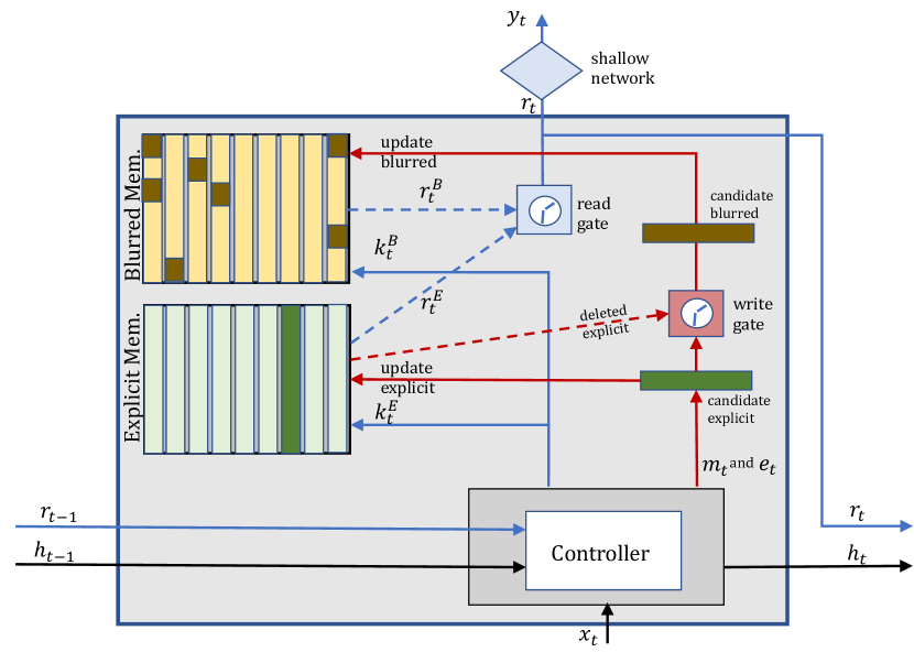
Figure 1. EBmRNN architecture: Memory controller processes observations and can choose to store them discretely in explicit memory block or as diffused higher level abstractions in blurred memory.

• a controller (e.g. a LSTM network) that processes inputs sequentially and produces candidate memory representation at each time point $t$ along with control vectors to manage the external memory. Mathematically, it can be expressed as follows:

  (1) $$\left[k_{t}^{E},k_{t}^{B},m_{t},e_{t}\right],h_{t}=RNN(h_{t-1},x_{t},r_{t-1})$$

• an ‘explicit’ memory bank, where the generated candidate memory representation is stored. Depending on the outputs of a controlling read gate, the candidate memory can be stored explicitly or passed on to the blurred memory. When it is stored explicitly and the bank was already full, an older memory is removed based on the information content and passed on to the blurred memory bank. To update the memory explicitly, we discretely select the index by make use of the Gumbel-Softmax trick as shown below:

  (2) $$\begin{array}[]{lcl}u_{t}&=&\alpha_{\mathcal{E}}u_{t-1}+(1-\alpha_{\mathcal{E}})w_{t}^{r,\mathcal{E}}\\ \gamma_{t}&=&\sigma\left(a_{\gamma}^{T}h_{t}+b_{\gamma}\right)\\ w_{t}^{w,\mathcal{E}}&=&\text{Gumbel-Softmax}\left(1-(\tilde{w}_{t}^{w,\mathcal{E}}+\gamma_{t}u_{t})\right)\\ \end{array}$$

  where, $u_{t}\in\mathbb{R}^{D}$ is a network learnt usage estimated. $\alpha_{\mathcal{E}}$ is a hyper-parameter capturing the effect of current reads on the slots and $w_{t}$ is a one-hot encoded weight vector over memory slots.

• The memory passed on to the blurred memory bank is diffused according to the control vectors and stored as high level concepts.

To generate outputs at time $t$, the architecture makes use of a read gate to select the memories stored in explicit and blurred memory that are useful at that time point.

(3) $$\begin{array}[]{lcl}g_{t}&=&\sigma\left(a^{\mathcal{B}T}_{g}r^{\mathcal{B}}_{t}+a^{\mathcal{E}T}_{g}r^{\mathcal{E}}_{t}+b_{g}\right)\\ r_{t}&=&\text{ReLU}\left((1-g_{t})\times W^{\mathcal{B}}_{r}r_{t}^{\mathcal{B}}+g_{t}\times W^{\mathcal{E}}_{r}r_{t}^{\mathcal{E}}+b_{r}\right)\par\end{array}$$

where, $\mathcal{B}$ and $\mathcal{E}$ are the blurred and explicit memories. $g_{t}\in\mathbb{R}$ is the read gate output and $r_{t}\in\mathbb{R}^{D}$ is the final output. The full model description is presented in the Appendix.

Experimental setup: We evaluated the performance of the proposed EBmRNN on the publicly available MIMIC III (Medical Information Mart for Intensive Care) data set (Johnson et al., 2016). The data includes vital signs, medications, laboratory measurements, observations and clinical notes. For this paper, we focused on the structured data fields and followed the MIMIC III benchmark proposed in (Harutyunyan et al., 2017) to construct cohorts for $3$ specific learning tasks of great interest to the critical care community namely, ‘In-hospital mortality’, ‘decompensation’, and ’phenotype’ classification. To estimate the effectiveness of the EBmRNN scheme, we compared it with the following baseline algorithms: Logistic Regression using the features used in (Harutyunyan et al., 2017), Long Short Term Memory Networks, and Gated Recurrent Unit (GRU) Networks. We also looked at a variant of EBmRNN that doesn’t have access to blurred memory, hereby referred to as EmRNN. Comparison with EmRNN allows the training to proceed via a direct path to explicit memories and hence estimate its effect more accurately. EmRNN is completely interpretable while EBmRNN is interpretable to the limit allowed by the complexities of the problem. Details on the exact cohort definitions and constructions are provided in (Harutyunyan et al., 2017). More details on the tasks are also presented in the Appendix.

Table 1. Performance comparison for $3$ classification tasks on test dataset.

	In-Hospital mortality	Decompensation	Phenotype
model	AUC-ROC	AUC-ROC	AUC-ROC(macro)	AUC-ROC(micro)
LR	0.8485	0.8678	0.7385	0.7995
LSTM	0.8542	0.8927	0.7670	0.8181
GRU	0.8575	0.8902	0.7664	0.8181
EmRNN	0.8507	0.8861	0.7670	0.8181
EBmRNN	0.8612	0.8989	0.7598	0.8191

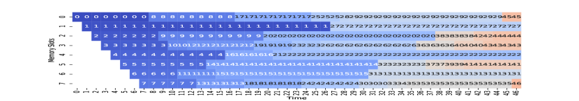
(a) In Hospital Mortality

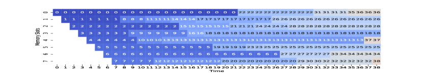
(b) Decompensation

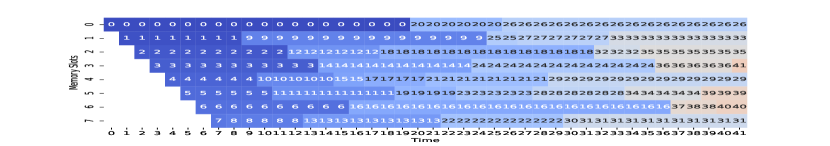
(c) Phenotyping

Figure 2. Case Study: Explicit memory slot utilization to store events for $3$ separate patients for $3$ tasks using $8$ slots for the memory. Each slot is annotated by the time index of the event stored in memory. Memory utilization patterns exhibit long-term dependency modeling.

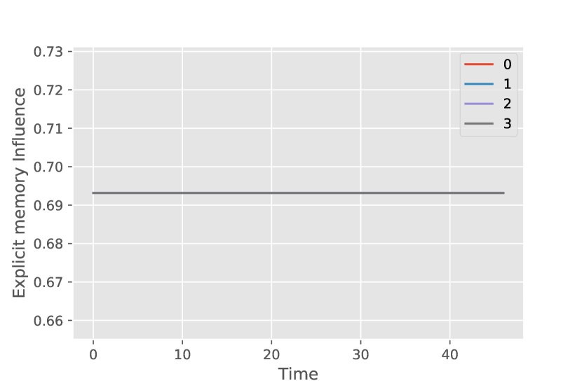
(a) In Hospital Mortality

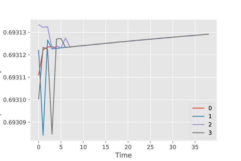
(b) Decompensation

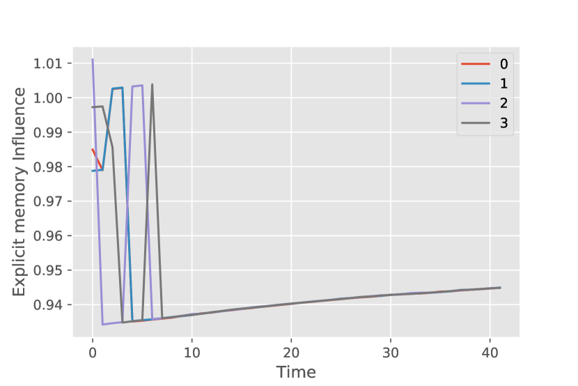
(c) Phenotyping

Figure 3. Case Study: Influence of explicit memory for $3$ tasks, $1$ patient per task, and $4$ hops of memory for read. The legends indicate the explicit memory influence for each of the hops. Influence patterns vary across tasks indicating the task complexity as well as the modeling flexibility of EBmRNN.

Data description: The dataset for each of the tasks is described below:
In Hospital Mortality Prediction: This task is a classification problem where the learning algorithm is asked to predict mortality using the first 48 hours of data collected on the patient for each ICU stay. All ICU stays for which the length of stay is unknown or less than 48 hours have been discarded from the study. Following exactly the benchmark cohort constructions proposed in (Harutyunyan et al., 2017), we were left with 17903 ICU stays for training and 3236 ICU stays for testing.

Decompensation Prediction: This task is a binary classification problem. Decompensation is synonymous to a rapid deterioration of health typically linked to very serious complications and prompting “track and trigger” initiatives by the medical staff. There are many ways to define decompensation. We adopt the approach used in (Harutyunyan et al., 2017) to represent the decompensation outcome as a binary variable indicating whether the patient will die in the next 24 hours. Consequently, data for each patient is labeled every hour with this binary outcome variable. The resulting data set for this task consists of 2,908,414 training instances and 523,208 testing instances as reported in (Harutyunyan et al., 2017) with a decompensation rate of 2.06

Phenotyping: This task is a multi label classification problem where the learning algorithm attempts to classify 25 common ICU conditions, including 12 critical ones such as respiratory failure and sepsis and 8 chronic comorbidities such as diabetes and metabolic disorders. This classification is performed at the ICU stay level, resulting in 35,621 instances in the training set and 6,281 instances in the testing set.

For each patient, the input data consists of an hourly vector of features containing average vital signs (e.g., heart rate, diastolic blood pressure), health assessment scores (e.g., Glasgow Come Scale) and various patient related demographics.

3. Results

All the models were trained for 100 epochs. We used the recommended setting for the baseline methods from (Harutyunyan et al., 2017). In this paper, we wanted to understand the relative importance of the memory banks and as such chose to study how the network uses the two different memory banks under similar capacity conditions. For EmRNN and EBmRNN, the hyperparameters such as the memory size ($4-32$), controller hidden size ($4-32$), and the number of reads ($2-8$) were set using the validation set for each of the different datasets. While $\alpha_{\mathcal{E}}$ can be learned during the training process, following past work, we used a fixed value of $0.7$. We chose a $2$-layered GRU with dropout as our controller and the models were trained using SGD with momentum ($0.9$) along with gradient clipping. Table 1 shows the AUC-ROC for the different tasks. Overall, we note that EBmRNN is on par or able to outperform each of the baselines for each of the tasks. Song et al. (Song et al., 2018) found success with a multi-layered large transformer based model and can be considered the state-of-the art including all architectures. It is interesting to note that our results, using a single layer of memory, are comparable to the many-layered transformer approach - thus indicating the efficiency of the proposed architecture. In the subsequent paragraphs, we discuss the key insights derived from the experiments.

How to interpret EBmRNN? To analyze the interpretability inherent in the model, we picked a patient for each of the tasks under consideration. We used a trained model with $8$ slots and allowing $4$ reads to generate the predictions. As mentioned before, the explicit memory allows complete traceability of inputs by storing each input in a distinct memory slot. Figure 2 depicts the contents of the explicit memory over time discretized by 1 hour. Such slot utilization pattern provides an insight into the contents recognized by the network as being important for the task at hand. Furthermore, the plots also exhibit that the model is able to remember, explicitly, far-off time points for an extended period, before caching it into the blurred memory space.

How to interpret the influence of explicit memory? In addition to exact memory contents, we can also analyze the importance of the explicit memory for specific tasks by analyzing the control for the read gate $g_{t}$ over time. Figure 3 shows the temporal progression of the read gate for the $3$ patients from previous analysis for three distinct tasks. Interestingly, we can see the model using different patterns of usage for different tasks. While the network is assigning almost equal importance to both banks for in hospital mortality, it is placing high importance on explicit memory for phenotyping. This can also correlate with the improved performance for EmRNN for the phenotyping task.

Why do we need the blurred memory? Given the interpretability provided by the explicit memory, it may be tempting to avoid the use of blurred memory in favor of EmRNN. As our results indicate, such a model can perform well for certain tasks. However, for tasks such as “in-hosptial mortality”, the blurred memory provides the network with additional capacity. Also, from a practical point of view, we found the EmRNN difficult to train where inspite of the Gumbel-Softmax reparameterization trick, the gradients frequently exploded and required higher supervision. On the other hand, the presence of the blurred bank helped the training by providing a more tractable path. If the use case demands a higher value for intepretability, we recommend to either use a smaller sized blurred memory bank or perform relative regularization of the read gates for the blurred component.

4. Conclusion

In this work, we have introduced EBmRNN, a memory network architecture able to mimic the human memory models by combining sensory, explicit and long term memories for classification tasks. The proposed scheme achieves state-of-the-art levels of performances while being more interpretable, especially when explicit memories are utilized more. Our future work will aim at presenting such interpretations via end-to-end system following a user centered design approach.

Appendix A Model Description

A.1. Explicit-Blurred Memory Augmented RNN

Let us denote the sequence of observations as $x=x_{1},x_{2},\cdots,x_{\mathcal{T}}$, where $\mathcal{T}$ is the length of the sequence and $x_{t}\in\mathbb{R}^{U}$. Similarly, let us denote the set of desired outputs as $y=y_{1},y_{2},\cdots,y_{\mathcal{T}},y_{t}\in\mathbb{R}^{V}$. To model $y$ from $x$, $x$ is fed sequentially to the proposed EBmRNN with parameters and hyper-parameters that will be defined below.

In EBmRNN, we split the conventional memory network architecture into two banks: (a) an explicit memory bank ($\mathcal{E}$) and (b) a blurred or diffused memory bank($\mathcal{B}$). Figure 1 shows a high level overview of the EBmRNN cell at time $t$. This cell has access to an explicit memory bank $\mathcal{E}\in\mathbb{R}^{N^{\mathcal{E}}\times D}$ to persist past events discretely. $N^{\mathcal{E}}$ denotes the capacity of the memory and $D$ is the dimensionality of each memory slot. This cell also has access to a blurred or diffused memory $\mathcal{B}\in\mathbb{R}^{N^{\mathcal{B}}\times D}$ where abstractions of important salient features from past observations are stored.

Observations at time $t$ are fed to this recurrent cell to produce an output $r_{t}\in\mathbb{R}^{D}$ based on the current input $x_{t}$, the external explicit and blurred memories $\mathcal{E}$ and $\mathcal{B}$. $r_{t}$ summarizes information extracted from both $\mathcal{E}$ and $\mathcal{B}$ that is deemed relevant for the generation of the output $y_{t}$. $r_{t}$ is designed to contain enough abstraction of past observations seen by EBmRNN, including the current input $x_{t}$ so that specific tasks can generate a desired $y_{t}$ using only a shallow network outside of the cell. This design choice helps the interpretability of the model as it facilitates linking $y_{t}$ to memories in $\mathcal{E}$ pointing explicitly to inputs $x_{t}$, while still retaining the expressiveness of a blurred memory. Analyzing how EBmRNN is using $\mathcal{E}$ provides a natural way to track how attentive EBmRNN is to input data stored in $\mathcal{E}$ while analyzing EBmRNN’s focus on $\mathcal{B}$ enables us to track the importance of long term dependencies. Details on how $r_{t}$ is computed are presented in the next subsection.

In addition to $\mathcal{E}$ and $\mathcal{B}$, there are three primary components controlling the functioning of the cell:

1. The controller ($\mathcal{C}$), that senses inputs to EBmRNN and maps these inputs into control signals for the management of all read and write operations to the memory banks.

2. The read gate controlling read accesses to the memory banks from control signals emitted by the controller.

3. The write gate controlling writes into the memory banks from control signals emitted by the controller.

In the remainder of this section, we describe these three components in details.

A.1.1. The Controller

At each time point $t$, the controller receives the current input $x_{t}$ and generates several outputs to manage $\mathcal{E}$ and $\mathcal{B}$ with appropriate read and write instructions sent to the read and write gates. As it receives $x_{t}$, the controller updates its hidden state $h_{t}\in\mathbb{R}^{C}$ based on the past output of the cell $r_{t-1}$ , its past hidden state $h_{t-1}$ and current input $x_{t}$. In addition to updating its hidden state $h_{t}$, the controller emits two keys $k_{t}^{\mathcal{E}}\in\mathbb{R}^{D}$ and $k_{t}^{\mathcal{B}}\in\mathbb{R}^{D}$ to be used by the read gate to control access to memory contents from $\mathcal{E}$ and $\mathcal{B}$. To control write operations, the controller also produces $m_{t}\in\mathbb{R}^{D}$ a representation of the $x_{t}$ that will be consumed by the write gate. $m_{t}$ represents information from $x_{t}$ that is candidate for a write into $\mathcal{E}$ and $\mathcal{B}$. The controller also produces $e_{t}\in\mathbb{R}^{D}$, an erased weight vector that will be consumed by the write gate to forget content from $\mathcal{B}$. In this work, we model the controller with standard recurrent neural network architectures such as Gated Recurrent Units (GRU) or Long Short Term Memory networks (LSTM). The operations of the controller are summarized below:

(4) $$\left[k_{t}^{E},k_{t}^{B},m_{t},e_{t}\right],h_{t}=RNN(h_{t-1},x_{t},r_{t-1})$$

A.1.2. The Read Gate and Read Operations

The read gate enforces read accesses from $\mathcal{E}$ and $\mathcal{B}$ by consuming $k_{t}^{\mathcal{E}}$ and $k_{t}^{\mathcal{B}}$ and comparing these keys against the content of the two memory banks $\mathcal{E}$ and $\mathcal{B}$. Using this addressing scheme, the following weight vectors over the memories are computed as follows:

(5) $$\begin{array}[]{lcl}w_{t}^{r,{\mathcal{B}}}&=&\text{Softmax}(S(k^{\mathcal{B}}_{t},\mathcal{B}_{t-1}))\\ w_{t}^{r,{\mathcal{E}}}&=&\text{Gumbel-Softmax}(S(k^{\mathcal{E}}_{t},\mathcal{E}_{t-1}))\\ \end{array}$$

where $S$ denotes an appropriate distance function between the key vectors and the memory locations. For our purpose, we use the cosine similarity measure as a distance function. $w_{t}^{r,{\mathcal{B}}}\in\mathbb{R}^{N^{\mathcal{B}}}$ and $w_{t}^{r,{\mathcal{E}}}\in\mathbb{R}^{N^{\mathcal{E}}}$. To ensure discrete access, $w_{t}^{r,{\mathcal{E}}}$ weights are required to be one-hot encoded vectors. While Softmax is a natural choice for soft selection of indices for $w_{t}^{r,{\mathcal{B}}}$, its use is not applicable for the hard selection required for $w_{t}^{r,{\mathcal{E}}}$. Gumbel Softmax is a newer paradigm that is applicable in this context compared to alternatives like top-K Softmax that can introduce discontinuities. Gumbel Softmax uses a stochastic re-parameterization scheme to avoid non-differentiablities that arise from making discrete choices during normal model training. We use the straight-through optimization procedure that allows the network to make discrete decisions on the forward pass while estimating the gradients on the backward pass using Gumbel Softmax. More details on this scheme can be found from (Gülçehre et al., 2017).

The read vectors $r^{\mathcal{E}}_{t}$ and $r^{\mathcal{B}}_{t}$ from each of the banks are computed as follows:

(6) $$r^{\mathcal{B}}_{t}=w_{t}^{r,\mathcal{B}}\mathcal{B}_{t-1}\quad\quad r^{\mathcal{E}}_{t}=w_{t}^{r,\mathcal{E}}\mathcal{E}_{t-1}$$

$r^{\mathcal{B}}_{t}$ and $r^{\mathcal{E}}_{t}$ belong both to $\mathbb{R}^{D}$. We combine the two content reads from the two banks using a gate as follows:

(7) $$\begin{array}[]{lcl}g_{t}&=&\sigma\left(a^{\mathcal{B}T}_{g}r^{\mathcal{B}}_{t}+a^{\mathcal{E}T}_{g}r^{\mathcal{E}}_{t}+b_{g}\right)\\ r_{t}&=&\text{ReLU}\left((1-g_{t})\times W^{\mathcal{B}}_{r}r_{t}^{\mathcal{B}}+g_{t}\times W^{\mathcal{E}}_{r}r_{t}^{\mathcal{E}}+b_{r}\right)\par\end{array}$$

$g_{t}\in\mathbb{R}$ while $r_{t}\in\mathbb{R}^{D}$. The final output from EBmRNN can then be produced from a shallow layer that combines the contribution from the two memory banks represented by $r_{t}$:

(8) $$y_{t}=\text{Softmax}\left(W_{y}r_{t}+b_{y}\right)$$

Equation 7 ensures that the network can learn to produce its desired output $y_{t}$ using information from either memory banks. The gated value $g_{t}$ controls the relative effect of the blurred and explicit memories on the output. On one hand, higher average values of $g_{t}$ would ensure that the network relies more on explicit memories and be as such easier to interpret. On the other hand, lower values of $g_{t}$ causes the network to rely more on blurred memories and be harder to interpret. Depending on the learning task at hand, there could be an interesting trade-off between learning performance and interpretability that can be controlled by this gating scheme. In fact, one could introduce a hyper-parameter in 7 to control this trade-off between $W^{\mathcal{B}}_{r}$ and $W^{\mathcal{E}}_{r}$.

The read operations are repeated $K$ times to generate $K$ hops from the memory.

A.1.3. The Write Gate and Write Operations

Once memories are read, the controller updates the memory banks for the next state. At each time point, the controller generates the memory representations, $m_{t}$, for the input $x_{t}$. The update strategy for the two banks are slightly different, and we start by describing the explicit bank update first.

Explicit memory update: As long as the explicit bank is not full, newer memories $m_{t}$ are simply appended to it and the update equation can be given as:

(9) $$\mathcal{E}_{t}=[\mathcal{E}_{t-1};m_{t}]$$

Once the entire memory is filled up, the network needs to learn to forget less important memory slots to generate a filtered explicit memory $\tilde{\mathcal{E}_{t-1}}$ and update the memory following equation 9. From an information theoretic intuition, more information can be retained by the network by sustaining a higher entropy within the memory banks. The network learns the importance of the old memories with respect to new memory candidate content $m_{t}$ as follows:

(10) $$\begin{array}[]{lcl}\tilde{w}_{t}^{w,{\mathcal{E}}}&=&\text{Softmax}(1-S(m_{t},\mathcal{E}_{t-1}))\\ \end{array}$$

$\tilde{w}_{t}^{w,{\mathcal{E}}}\in\mathbb{R}^{N^{\mathcal{E}}}$. Equation 10 only uses the content to generate the importance of the memory locations. Specifically, interpreting these values of $\tilde{w}_{t}^{w,{\mathcal{E}}}$ in terms of retention probabilities, locations with dissimilar contents will have higher retention probability - thereby forcing the network to store discriminative content in the explicit memory.

Past research has also shown that usage-based addressing can significantly improve the expressiveness of the network. We follow the scheme proposed by (Gülçehre et al., 2017) and make use of an auxiliary variable $u_{t}$ that tracks a moving average of past read values for each memory locations of $\mathcal{E}$. The final write vector along with all the usage update is given as:

(11) $$\begin{array}[]{lcl}u_{t}&=&\alpha_{\mathcal{E}}u_{t-1}+(1-\alpha_{\mathcal{E}})w_{t}^{r,\mathcal{E}}\\ \gamma_{t}&=&\sigma\left(a_{\gamma}^{T}h_{t}+b_{\gamma}\right)\\ w_{t}^{w,\mathcal{E}}&=&\text{Gumbel-Softmax}\left(1-(\tilde{w}_{t}^{w,\mathcal{E}}+\gamma_{t}u_{t})\right)\\ \end{array}$$

$u_{t}\in\mathbb{R}^{D},\gamma_{t}\in\mathbb{R},w_{t}^{w,\mathcal{E}}\in\mathbb{R}^{N^{\mathcal{E}}}$. $\alpha_{\mathcal{E}}$ is a hyper-parameter capturing the effect of current reads on the slots.

Although, other addressing mechanisms have been proposed in literature, we chose this setting for model simplicity and also to better capture the desirable properties of EHR applications.

The explicit bank $\mathcal{E}$ is then updated by removing the slot with the highest value of $w_{t}^{w,\mathcal{E}}$ ($\hat{m}_{t}$ from slot $j$) and replacing its content with $m_{t}$. At that time, we also reset the usage value for the slot (i.e. $u_{t}[j]=0$).

Similar to the read operations, $w_{t}^{w,E}$ is a one-hot encoded vector, the equations for the popped memory, and subsequently update of the explicit memory are given as below:

(12) $$\begin{array}[]{lcl}\hat{m_{t}}&=&\mathcal{E}_{t-1}w_{t}^{w,\mathcal{E}}\\ \mathcal{E}_{t}&=&\mathcal{E}_{t-1}\circ(1_{N^{\mathcal{W}}\times D}-w_{t}^{w,\mathcal{E}}1_{D})+w_{t}^{w,\mathcal{E}}m^{\mathcal{E}}_{t}\\ \end{array}$$

where $1_{N^{\mathcal{W}}\times D}$ represents a $N^{\mathcal{W}}\times D$ matrix of all 1 and $1_{D}$ represents the same for a $D$ dimensional vector.

Blurred memory update: The Blurred memories are used to represent past events with more abstract concepts that can capture long term dependencies. The memory bank $\mathcal{B}$ provides a place for memories forgotten from the explicit bank to be stored in more abstract sense. $\mathcal{B}$ also allows EBmRNN to track and access a higher dimensional construct of current memory representation.

We generate a candidate blurred memory using the following equation:

(13) $$\begin{array}[]{lcl}f_{t}&=&\sigma(W^{i}_{f}m_{t}+W^{\mathcal{E}}_{f}\hat{m}_{t}+b_{f})\\ m^{\mathcal{B}}_{t}&=&\text{ReLU}((1-f_{t})W_{i}m_{t}+f_{t}W_{\mathcal{E}}\hat{m}_{t}+b_{m})\\ \end{array}$$

We generate write-vectors $w_{t}^{w,\mathcal{B}}$ using a formulation similar to equation 10 by replacing the Gumbel-Softmax with a Softmax. The final update equation for the blurred memory can then be given as follows:

(14) $$\begin{array}[]{lcl}\tilde{w}_{t}^{w,{\mathcal{B}}}&=&\text{Softmax}(S(m^{\mathcal{B}}_{t},\mathcal{B}_{t-1}))\\ \mathcal{B}_{t}&=&\mathcal{B}_{t-1}\circ(1_{N\times W}-w_{t}^{w,\mathcal{B}}e_{t})+w_{t}^{w,\mathcal{B}}m^{\mathcal{B}}_{t}\end{array}$$

where $e_{t}$ is an erase weight generated by the controller.

References

- (1)
- Atkinson and Shiffrin (1968) R. C. Atkinson and R. M. Shiffrin. 1968. Human memory: A proposed system and its control processes. In K. W. Spence and J. T. Spence (Eds.), The Psychology of learning and motivation: Advances in research and theory (vol. 2). (1968), 89 – 105.
- Graves et al. (2014) Alex Graves, Greg Wayne, and Ivo Danihelka. 2014. Neural Turing Machines. CoRR abs/1410.5401 (2014). http://dblp.uni-trier.de/db/journals/corr/corr1410.html#GravesWD14
- Graves et. al. (2016) Alex Graves et. al. 2016. Hybrid computing using a neural network with dynamic external memory. Nature 538, 7626 (Oct. 2016), 471–476. http://dx.doi.org/10.1038/nature20101
- Gülçehre et al. (2017) Çaglar Gülçehre, Sarath Chandar, and Yoshua Bengio. 2017. Memory Augmented Neural Networks with Wormhole Connections. CoRR abs/1701.08718 (2017). arXiv:1701.08718 http://arxiv.org/abs/1701.08718
- Gulcehre et al. (2018) Caglar Gulcehre, Sarath Chandar, Kyunghyun Cho, and Y Bengio. 2018. Dynamic Neural Turing Machine with Continuous and Discrete Addressing Schemes. Neural Computation 30 (01 2018), 1–28. https://doi.org/10.1162/neco_a_01060
- Harutyunyan et al. (2017) Hrayr Harutyunyan, Hrant Khachatrian, David C. Kale, and Aram Galstyan. 2017. Multitask Learning and Benchmarking with Clinical Time Series Data. CoRR abs/1703.07771 (2017). http://dblp.uni-trier.de/db/journals/corr/corr1703.html#HarutyunyanKKG17
- Jain and Wallace (2019) Sarthak Jain and Byron C Wallace. 2019. Attention is not Explanation. In Proceedings of the 2019 Conference of the North American Chapter of the Association for Computational Linguistics: Human Language Technologies, Volume 1 (Long and Short Papers). 3543–3556.
- Johnson et al. (2016) Alistair E.W. Johnson, Tom J. Pollard, Lu Shen, Li-wei H. Lehman, Mengling Feng, Mohammad Ghassemi, Benjamin Moody, Peter Szolovits, Leo Anthony Celi, and Roger G. Mark. 2016. MIMIC-III, a freely accessible critical care database. Scientific Data 3 (2016), sdata201635. https://doi.org/10.1038/sdata.2016.35
- Le et al. (2018) Hung Le, Truyen Tran, and Svetha Venkatesh. 2018. Dual memory neural computer for asynchronous two-view sequential learning. In Proceedings of the 24th ACM SIGKDD International Conference on Knowledge Discovery & Data Mining. ACM, 1637–1645.
- Prakash et al. (2017) Aaditya Prakash, Siyuan Zhao, Sadid A Hasan, Vivek V Datla, Kathy Lee, Ashequl Qadir, Joey Liu, and Oladimeji Farri. 2017. Condensed Memory Networks for Clinical Diagnostic Inferencing.. In AAAI. 3274–3280.
- Song et al. (2018) Huan Song, Deepta Rajan, Jayaraman J Thiagarajan, and Andreas Spanias. 2018. Attend and diagnose: Clinical time series analysis using attention models. In Thirty-Second AAAI Conference on Artificial Intelligence.
- Sukhbaatar et al. (2015) Sainbayar Sukhbaatar, Arthur Szlam, Jason Weston, and Rob Fergus. 2015. End-To-End Memory Networks. In Proceedings of the International Conference on Neural Information Processing Systems (NIPS). https://doi.org/v5 arXiv:1503.08895
- Sun et. al. (2012) Jimeng Sun et. al. 2012. Combining knowledge and data driven insights for identifying risk factors using electronic health records. In AMIA Annual Symposium Proceedings, Vol. 2012. American Medical Informatics Association, 901.
- Tomašev et al. (2019) Nenad Tomašev, Xavier Glorot, Jack W Rae, Michal Zielinski, Harry Askham, Andre Saraiva, Anne Mottram, Clemens Meyer, Suman Ravuri, Ivan Protsyuk, et al. 2019. A clinically applicable approach to continuous prediction of future acute kidney injury. Nature 572, 7767 (2019), 116.
- Xiao et al. (2018) Cao Xiao, Tengfei Ma, Adji B Dieng, David M Blei, and Fei Wang. 2018. Readmission prediction via deep contextual embedding of clinical concepts. PloS one 13, 4 (2018), e0195024.