Optimal Mini-Batch Size Selection for Fast Gradient Descent

Abstract

This paper presents a methodology for selecting the mini-batch size that minimizes Stochastic Gradient Descent (SGD) learning time for single and multiple learner problems. By decoupling algorithmic analysis issues from hardware and software implementation details, we reveal a robust empirical inverse law between mini-batch size and the average number of SGD updates required to converge to a specified error threshold. Combining this empirical inverse law with measured system performance, we create an accurate, closed-form model of average training time and show how this model can be used to identify quantifiable implications for both algorithmic and hardware aspects of machine learning. We demonstrate the inverse law empirically, on both image recognition (MNIST, CIFAR10 and CIFAR100) and machine translation (Europarl) tasks, and provide a theoretic justification via proving a novel bound on mini-batch SGD training.

Introduction

In this paper, we present an empirical law, with theoretical justification, linking the number of learning iterations to the mini-batch size. From this result, we derive a principled methodology for selecting mini-batch size w.r.t. training performance for data-parallel machine learning. This methodology saves training time and provides both intuition and a principled approach for optimizing machine learning algorithms and machine learning hardware system design. Further, we use our methodology to show that focusing on weak scaling can lead to suboptimal training times because, by neglecting the dependence of convergence time on the size of the mini-batch used, weak scaling does not always minimize the training time. All of these results derive from a novel insight presented in this paper, that understanding the average algorithmic behavior of learning, decoupled from hardware implementation details, can lead to deep insights into machine learning.

Our results have direct relevance to on-going research that accelerate training time. For example, significant research effort has been focused on accelerating mini-batch SGD (?; ?; ?), primarily focused on faster hardware (?; ?; ?; ?), parallelization using multiple learners (?; ?; ?), and improved algorithms and system designs for efficient communication (e.g., parameter servers, efficient passing of update vectors (?; ?; ?; ?; ?; ?; ?), etc. To assess the impact of these acceleration methods, published research typically evaluates parallel improvements based on the time to complete an epoch for a fixed mini-batch size, what is commonly known as “weak” scaling (?; ?; ?; ?).

The next section explains how the insight of decoupling algorithmic and implementation details is used to develop a close-form model for learning convergence time. We then derive implications for hardware system design. These implications are followed by sections with experimental support and theoretical justification for the empirical law connecting learning iterations with mini-batch size. We close with a discussion section.

Modeling SGD Convergence Time

Given a learning problem represented by a data set, SGD as the learning algorithm, and a learning model topology, we define the learning time, $T_{\rm{C}}$, to be the average total time required for SGD to converge to a specified achievable training error threshold. The average is over all possible sources of randomness in the process, including random initializations of the model, “noise” from the SGD updates, noise in the system hardware, etc. Focusing on the average learning behavior allows us to identify fundamental properties of the learning process. In particular, we can write the analytical complexity as the product of iteration complexity, $N_{\rm{Update}}$, and the per iteration computational complexity, $T_{\rm{Update}}$.

$$T_{\rm{C}}=N_{\rm{Update}}\cdot T_{\rm{Update}}$$ (1)

In other words, $N_{\rm{Update}}$ is the average number of updates required to converge, and $T_{\rm{Update}}$ is the average time to compute and communicate one update.

This decomposition of $T_{\rm{C}}$ into an implementation-dependent and implementation-independent components is useful because it helps decouple the tasks of understanding how implementation and algorithmic choices impact learning time, and allows us to understand algorithmic choices, independent of system design choices.

Modeling Average Convergence Time

To analyze SGD convergence, we model $N_{\rm{Update}}$ as a function of the mini-batch size, $M$, and model $T_{\rm{Update}}$ as a function of $M$ and the number of parallel learners, $P$. All other hyperparameters are held constant.

For simplicity, we refer to “learner” parallelism when multiple learners share the task of learning a single model. Each learner is mapped to a compute element from a suitable level of parallelism, e.g., a server, a CPU, a GPU, etc.

In general, the level of parallelism selected will have implications for the software implementation, communication requirements, and system performance. However, our analysis below is independent of these details.

Modeling $N_{\rm{Update}}(M)$

Since $N_{\rm{Update}}$ is independent of the hardware, it is independent of the number of compute elements used, and therefore depends only on the mini-batch size, $M$. Even with this simplification, measuring $N_{\rm{Update}}$ from hardware is generally impractical due to the computational expense of running SGD to convergence for all values of $M$. Fortunately, there is an easier way: We have discovered a robust empirical inverse relationship between $N_{\rm{Update}}$ and $M$ given by

$$N_{\rm{Update}}=N_{\infty}+\frac{\alpha}{M}$$ (2)

where $N_{\infty}$ and $\alpha$ are empirical parameters depending on the data, model topology and learning algorithm used.

This inverse relationship captures the intuitively obvious result that even if we compute exact gradients, i.e., even when $M$ equals all of the data in a given data set, gradient descent still requires a non-zero number of steps to converge.

Furthermore, the Central Limit Theorem tells us that the variance of the SGD gradient is inversely proportional to $M$, for large $M$. Thus, $N_{\rm{Update}}$ increases approximately linearly with the SGD gradient variance, and $\alpha$ can be thought of the system’s sensitivity to noise in the gradient. We define $\alpha$ to be the “noise sensitivity” of the algorithm.

Novelty of this Result

Numerous papers have addressed the behavior and benefits of mini-batch training (?; ?; ?). These papers frequently derive training error bounds in terms of the number of iterations, and/or the mini-batch size, often exhibiting $1/M$ and $1/N$ related behavior. Although these results superficially look similar to Eqn. 2, they do not address the functional relationship between the number of iterations and $M$. Our work is the first to demonstrate this relationship empirically, on a wide variety of learning problems, in a much simpler way. Furthermore, for some of the results in (?; ?; ?), it is possible to go beyond what the original authors intended by inverting their results to find relationships between number of iterations and $M$; however, without empirical evidence, one does not know how tight the bounds are in practice, and even if one assumes they are tight, the resulting inversion leads to relationships which are not the same as Eqn. 2.

To make this explicit with an example, consider the second equation on P. 31 of (?) which, with simplified notation and constants $A$ and $B$, can be written as

$$E_{N}\leq A/M+(1-B/M)^{N-1}(E_{1}-A/M)$$

If we replace $E_{N}$ with a target error threshold, $\epsilon$, this equation implies the following inequality:

$$N\geq 1+\frac{M}{M-B}\ln\left(\frac{\epsilon M-A}{E_{1}M-A}\right)$$

which is clearly different from Eqn. 2. One can perform similar analyses to the other published results to demonstrate that they are not equivalent Eqn. 2.

Modeling $\mathbf{T_{\rm{Update}}(M,P)}$

Measuring $T_{\rm{Update}}$ is comparatively straightforward: One need only run enough iterations of SGD for a single learner to estimate the average time to perform an update for a specified mini-batch size. This process is possible because $T_{\rm{Update}}(M,P)$ is approximately constant throughout SGD learning. This approach can be used to compare differences between specific types of hardware, software implementations, etc. One then use the measured $T_{\rm{Update}}$ to fit an analytic model, along with $N_{\rm{Update}}$, to model $T_{\rm{C}}(M,P)$.

To analyze the generic behavior, we model

$$T_{\rm{Update}}(M,P)=\Gamma(M)+\Delta(P)$$ (3)

where $\Gamma(M)$ is the average time to compute an SGD update using $M$ samples, and $\Delta(P)$ is the average time to communicate gradient updates between $P$ learners. If some of the communication between learners can occur during computation, then $\Delta(P)$ represents the portion of communication that is not overlapping with computation. Since computation and communication are handled by separate hardware, it is a good approximation to assume that they can be decoupled in this way.

Since $\Gamma(M)$ typically performs the same amount of computation for each data sample, one might expect a linear relationship, $\Gamma(M)=\gamma M$, for some constant, $\gamma$. However, in practice, hardware and software implementation inefficiencies lead to a point where reducing $M$ does not reduce compute time linearly. This effect can be approximated using

$$\Gamma(M)=\gamma\max(M,M_{T})$$ (4)

where $M_{T}$ is the threshold at which the linear relationship begins, i.e., the knee in the curve. For example, $M_{T}$ could be the number of cores per CPU, if each sample is processed by a different core; or $M_{T}$ could be 1 if a single core processes all samples. Ideally, efficient SGD hardware systems should achieve low $\gamma$ and $M_{T}$. In practice, an empirical measurement of this relationship provides more fidelity; but for the purposes of this paper, this model is sufficient.

For $P=1$, the communication time is zero, i.e., $\Delta(P)=0$. For $P>1$, $\Delta(P)$ depends on various hardware and software implementation factors. We assume model updates exploit an optimized communication protocol, such as the Message Passing Interface (MPI) function MPIAllReduce() (?) on a high-end compute cluster. Such systems provide a powerful network switch and an efficient MPIAllReduce() implementation that delivers near perfect scaling of MPIAllreduce() bandwidth, and so communication time is approximately constant, i.e., $\Delta(P)=\delta$ for some constant $\delta$ approximately inversely proportional to the aggregate bandwidth between learners. For comparison purposes, a synchronous parameter server has a communication time that grows linearly with $P$, i.e., $\Delta(P)=\delta P$.

Modeling $\mathbf{T_{\rm{C}}(M,P)}$

Using Eqn. 1 to combine our estimates for $N_{\rm{Update}}$, $T_{\rm{Update}}$ yields the following general approximation to the total convergence time for SGD running on $P$ parallel learners:

$$T_{\rm{C}}(M,P)=\left(N_{\infty}+\frac{\alpha}{M}\right)\left[\gamma\max\left(\frac{M}{P},M_{T}\right)+\delta\right]$$ (5)

We can now use this model to optimize training time and analyze the impact of system design on training time in numerous ways. E.g., in the experiments we show how to select the mini-batch size that minimizes SGD training time.

Note that Eqn. 5 relies on certain assumptions about the hardware that might not be true in general, e.g., that $\delta$ is a constant. We have chosen these assumptions to simplify the analysis; but in practice, one can easily choose a different model for $T_{\rm{C}}$, or even measure the exact form of $T_{\rm{C}}$, and still follow through with the analysis below.

One final consideration arises regarding cross-validation (CV) since SGD training is rarely performed without some form of CV stopping criterion. We can accommodate the effect of CV in our model by including a CV term, such that

$$\Gamma(M)=\gamma N\max(M,M_{T})+\gamma_{\rm CV}\max(M_{\rm CV},M_{T})$$ (6)

where $N$ is the number of SGD updates per CV calculation and $M_{\text{CV}}$ is the number of CV samples to calculate. For simplicity, we ignore CV in our analysis below, but the analysis follows the same path as before. Additionally, the calculation of a CV subset adds virtually no communication, since the parallel learners computing the CV estimate communicate only a single number when they are done.

Optimal Mini-Batch Size Selection

For the single learner case ($P=1$), there is no inter-learner communication cost, so Eqn. 5 yields

$$T_{\rm{C}}(M,1)=\left(N_{\infty}+\frac{\alpha}{M}\right)\gamma\max\left(M,M_{T}\right).$$ (7)

Optimizing over $M$, we find the optimal mini-batch size to be

$$M_{\rm Opt}=M_{T}.$$ (8)

One can easily identify $M_{T}$ for a given system by timing a few SGD updates per value of $M$ to obtain an estimate of $T_{\rm{Update}}(M)$, and then selecting the knee in the $T_{\rm{Update}}(M)$ curve as an estimate for $M_{T}$. If the simple model used in Eqn. 4 is not accurate for a given system configuration, the methodology below can be used.

Methodology: Optimal Mini-Batch Size Selection
1.	For a range of $M$ values:
	Measure $T_{\rm{Update}}(M)$ over a few SGD updates.
2.	For a least two values of $M$:
	Estimate $N_{\rm{Update}}(M)$ by running to convergence.
3.	Fit $N_{\infty}$ and $\alpha$ to estimate $N_{\rm{Update}}(M)$ values.
4.	Use $N_{\rm{Update}}(M,N_{\infty},\alpha)$, $T_{\rm{Update}}(M)$ to select $M_{\rm Otp}$.

For the multiple learning case ($P\geq 1$), the optimal $M$ is given by

$$M_{\rm Opt}(P)=\max\left(\sqrt{\frac{\alpha\delta P}{N_{\infty}\gamma}}~{}~{},~{}~{}M_{T}P\right)$$ (9)

which demonstrates that linearly increasing the training data with the number of learners (i.e., “weak scaling”) is not always the optimal choice because $M_{T}P$ can be less than $\sqrt{\alpha\delta P/N_{\infty}\gamma}$. Note that the methodology above can also be used to optimize $M$ in the multi-learner case.

Data Parallel Scaling of Parallel SGD

Scaling measures the total time to solution, as a function of the number of computer nodes. Traditionally, there are two scaling schemes, Strong Scaling and Weak Scaling. We discuss these below and note that neither is ideal for SGD-based machine learning. We therefore introduce Optimal Scaling and compare the three approaches.

Our analysis assumes data parallelism, which leads to node-level load imbalance (and corresponding inefficiency) when the minibatch size is not a multiple of the number of nodes, $P$. For convenience, the analysis below ignores these effects and thus presents a slightly more optimistic analysis.

Strong Scaling

Strong scaling occurs when the problem size remains fixed. This means that the amount of compute per node decreases as $P$ increases. For training tasks, this implies that $M$ is fixed, i.e., $M=M_{\rm Strong}$. In this case, $N_{\rm{Update}}$ does not change, so the training time improves only when $T_{\rm{Update}}$ decreases. Thus, strong scaling hits a minimum when $P>M_{\rm Strong}/M_{T}$.

Weak Scaling

Weak scaling occurs when the problem size grows proportionately with $P$. This implies that for training tasks, $M$ grows linearly with $P$ (i.e., $M=mP$) and therefore $N_{\rm{Update}}$ decreases as $P$ increases, while $T_{\rm{Update}}$ remains constant, for constant $m$. Weak scaling can be optimized by selecting $m$ appropriately, which leads to the optimal scaling described below.

Optimal Scaling

The constant $M$ of strong scaling and the linear $M$ of weak scaling prevent these methods from achieving optimal performance, and are therefore inappropriate for SGD-based machine learning. We propose an alternative approach to scaling that, unlike strong and weak scaling, minimizes $T_{\rm{C}}(M,P)$ over $M$ for each value of $P$. This approach allows better performance than either strong or weak scaling.

If we combine Eqn. 5 with Eqn. 9, we get a closed for solution for the minimum time to convergence:

$$T_{\rm{C}}(P)=\begin{cases}\left(\sqrt{\delta N_{\infty}}+\sqrt{\frac{\alpha\gamma}{P}}\right)^{2},&P<\frac{\alpha\delta}{\gamma M_{T}^{2}N_{\infty}}\\ \left(N_{\infty}+\frac{\alpha}{M_{T}P}\right)\left(\delta+\gamma M_{T}\right),&{\rm otherwise.}\end{cases}$$ (10)

Note that for large $P$ (i.e., the second condition above), optimal scaling is identical to weak scaling. In this way, optimal scaling naturally defines the per node minibatch size for weak scaling.

Optimal System Hardware Design

We now show how optimal scaling can be used to optimize learning system hardware design. The principle behind optimal system design is to balance the trade-offs between various system parameters so as to optimize some system performance metric, like time to convergence. If we assign a cost for each system component, such as the number of nodes, the size of the communication network, the amount of memory, etc., we can then find the value of these elements that optimize the system metric. This approach can be used to optimize system design for multiple machine learning problems, e.g., determining the correct ratio of compute to communication in a system; or to efficiently allocate resources in a data center running multiple learning problem concurrently, e.g., to decide how many learners to apply to each learning task running in a data center.

To make this explicit, consider optimizing a system for bandwidth and compute only. If we have a fixed amount of money to spend, then the cost, $C$, for each component must be constrained by

$$C_{\rm Compute}(P,\gamma)+C_{\rm Bandwidth}(\delta)={\rm constant.}$$ (11)

Combining this constraint with $T_{\rm{C}}$ implies that optimal design occurs when the mix of compute and bandwidth satisfy

$$\frac{{\Delta}T_{\rm{C}}(M_{\rm Opt}(P),P,\gamma)}{{\Delta}C_{\rm Compute}(P,\gamma)}=\frac{{\Delta}T_{\rm{C}}(M_{\rm Opt}(P),P,\gamma)}{{\Delta}C_{\rm Bandwidth}(\delta)}.$$ (12)

In other words, performance gain per unit price must be balanced at the optimal design point. Since we have a closed form solution for $T_{\rm{C}}$, we can easily find this optimal point if given the various costs. This approach can be generalized to optimize of multiple constraints.

Experimental Results

We have observed that, to a reasonable approximation, the relationship

$$N_{\rm{Update}}=N_{\infty}+\frac{\alpha}{M}$$ (13)

persists over a broad range of $M$, and a variety of machine learning dimensions, including the choice of learning domain (image recognition and machine translation), data set, model topology, number of classes, convergence threshold and learning rate. This section describes the methodology used to assess this relationship and the results obtained.

Table 1: Image recognition rraining experiments performed.

Data Set	Model	# Parameters	# Layers	Learning Rate	$M$
MNIST	Small – LeNet (?)	43,158	4	0.01	1 - 1024
	Medium – LeNet (?)	169,506	4	0.01, 0.05	1 - 1024
	Even/Odd – LeNet (?)	169,506	4	0.05	1 - 1024
	Large – LeNet (?)	671,802	4	0.01	1 - 1024
CIFAR10	Small – LeNet (?)	487,458	4	0.05	1 - 1024
	Medium – VGG (?)	1,125,090	9	0.01, 0.05, Adam	1 - 1024
	Large – VGG (?)	1,862,754	11	0.025	1 - 1024
	ResNet (?)	270,410	20	0.05	1 - 1024
CIFAR100	Small – LeNet (?)	487,458	4	0.05	16 - 1024
	Medium – VGG (?)	1,125,090	9	0.05	16 - 1024
	Large - VGG (?)	1,862,754	11	0.025, 0.05	16 - 1024

Image Recognition Task

To measure the robustness of our observations for image recognition, we conducted a range of experiments as described in Table 1. Adam (?) adaptive learning rate was also used for one of the models. Light regularization was used with a decay constant of $10^{-4}$ on the $L_{2}$-norm of the weights. For each model architecture, we varied the size in terms of width (i.e., parameters per layer) and depth (i.e., number of layers) to measure the training behavior across model topologies. In addition, we experimented with the same model across all three data sets (LeNet). Training was performed using the Torch library on a single K80 GPU. Training and cross-validation losses were recorded after each update for MNIST and after every 100 updates for CIFAR10 and CIFAR100, using two distinct randomly selected sets of 20% of the available data. The recorded results were “scanned” to find the $T_{\rm{Update}}$ value that first achieves the desired training loss level, $\epsilon$. This approach is equivalent to a stopping criterion with no patience.

Each MNIST experiment was averaged over ten runs with different random initializations to get a clean estimate of $N_{\rm{Update}}$ as a function of $M$. Averaging was not used with the other experiments, and as our results show, was not generally needed.

The results of our experiments in Figure 1 show a robust inverse relationship between $N_{\rm{Update}}$ and $M$ measured across all the data sets, models, learning rates for each case we have considered. The fit lines match the observed data closely and we estimated $N_{\infty}$ and $\alpha$. Because of the large number of possible combinations of experiments performed, we only show a representative subset of the graphs to illustrate the behavior that was observed in all experiments. This empirical behavior exists for training error, cross-validation error, varying $\epsilon$, changing the number of output classes, etc.

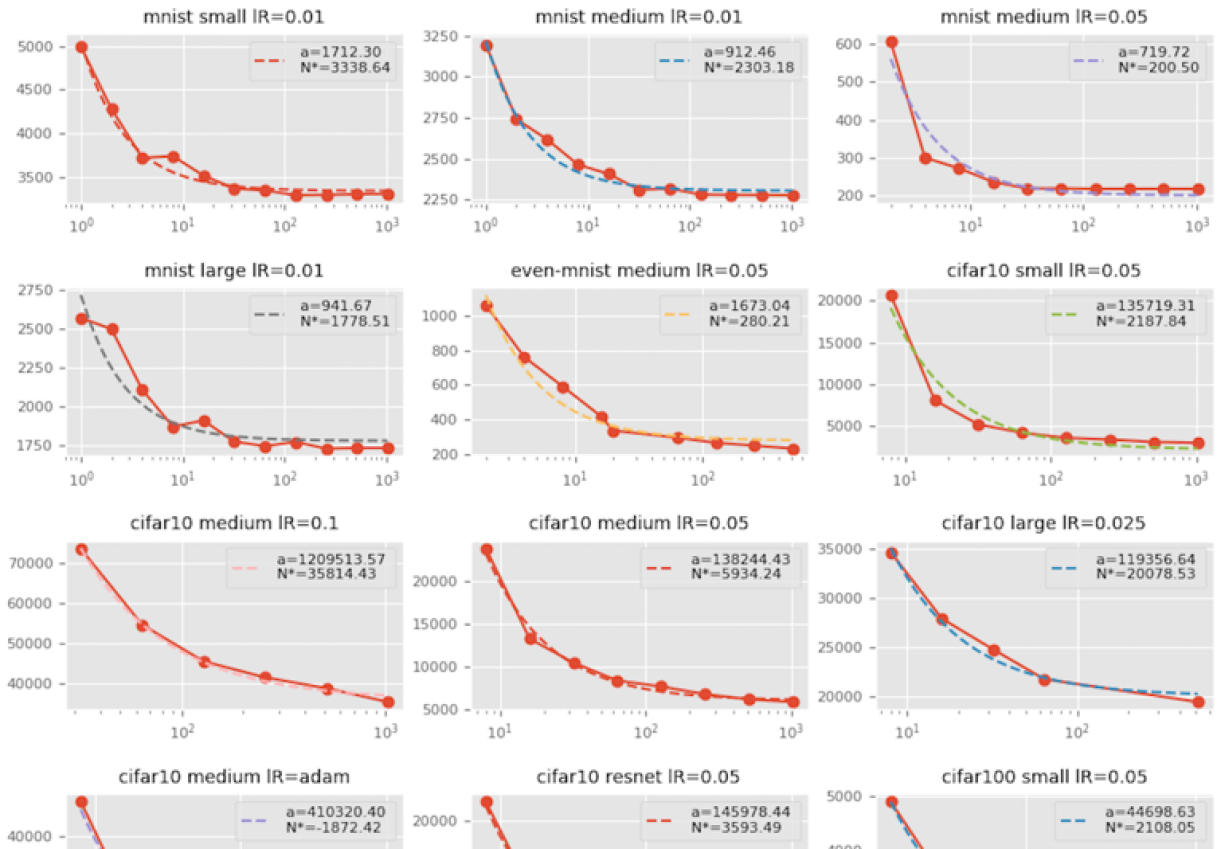
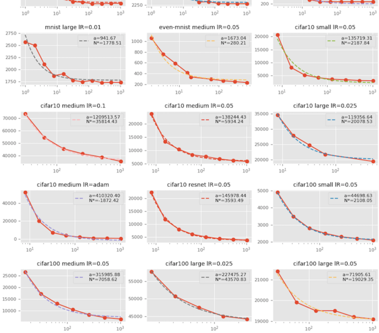
Figure 1: $N_{\rm{Update}}$ as a function of $M$ for a variety of SGD learning problems for a variety of conditions. The y-axis represents the training loss. The plots generally show an inverse relationship between $N_{\rm{Update}}$ and $M$. Since $N_{\rm{Update}}$ is a random variable, we see noise in these graphs. Additional averaging over multiple runs removes this noise.

These results show that large learning rates (shown as “lR” in the graphs) are associated with small $N_{\infty}$, which is not unexpected. However, for the experiment with adaptive learning rate (cifar10_medium_adam), $N_{\infty}$ is negative, which is likely the result of noise in our estimates or a failure of the model for adaptive learning rates. Further study is needed to understand this. Even so, this indicates that $N_{\infty}$ is small compared to the $\alpha$, and hence good parallel efficiency is possible.

Machine Translation Task

Our translation system implements the attentional model of translation (?) consisting of an encoder-decoder network with an attention mechanism. The encoder uses a bidirectional GRU recurrent neural network (?) to encode a source sentence ${\bf{x}}=(x_{1},...,x_{l})$, where $x_{i}$ is the embedding vector for the $i$th word and $l$ is the sentence length. The encoded form is a sequence of hidden states ${\bf{h}}=(h_{1},...,h_{l})$ where each $h_{i}$ is computed as follows

$$h_{i}=\begin{bmatrix}\overleftarrow{{h}_{i}}\\ \overrightarrow{{h}_{i}}\end{bmatrix}=\begin{bmatrix}\overleftarrow{f}(x_{i},\overleftarrow{h}_{i+1})\\ \overrightarrow{f}(x_{i},\overrightarrow{h}_{i-1})\end{bmatrix},$$ (14)

where $\overrightarrow{h_{0}}=\overleftarrow{h_{0}}=0$. Here $\overleftarrow{f}$ and $\overrightarrow{f}$ are GRU cells.

Given $\bf{h}$, the decoder predicts the target translation ${\bf y}$ by computing the output token sequence $(y_{1},...y_{m})$, where $m$ is the length of the sequence. At each time $t$, the probability of each token $y_{t}$ from a target vocabulary is

$$p(y_{t}|{\bf h},y_{t-1}..y_{1})=g(s_{t},y_{t-1},H_{t}),$$ (15)

where $g$ is a two layer feed-forward network over the embedding of the previous target word ($y_{t-1}$), the decoder hidden state ($s_{t}$), and the weighted sum of encoder states ${\bf h}$ ($H_{t}$), followed by a softmax to predict the probability distribution over the output vocabulary. We use a two layer GRU for $s_{t}$. The two GRU units together with the attention constitute the conditional GRU layer of (?). $H_{t}$ is computed as

$$H_{t}=\begin{bmatrix}\sum^{l}_{i=1}(\alpha_{t,i}\cdot\overleftarrow{h}_{i})\\ \sum^{l}_{i=1}(\alpha_{t,i}\cdot\overrightarrow{h}_{i})\end{bmatrix},$$ (16)

where $\alpha_{t,i}$ are the elements of $\alpha_{t}$ which is the output vector of the attention model. This is computed with a two layer feed-forward network

$$\alpha^{\prime}_{t}=v(\textrm{tanh}(w(h_{i})+u(s^{\prime}_{t-1}))),$$ (17)

where $w$ and $u$ are weight matrices, and $v$ is another matrix resulting in one real value per encoder state $h_{i}$. $\alpha_{t}$ is then the softmax over $\alpha^{\prime}_{t}$.

We train our MT model with the Pytorch framework (?). Learning is performed with the Pytorch implementation of SGD. No adjustment to learning rates was performed. We used the Europarl (?) German-English data set for training and newstest2013 data set for testing.

For our experiments, we trained with mini-batch sizes of 100, 200, 400, 800, 1600, 3200, and 6400 words per mini-batch. 12800 was too large for GPU memory. Each mini-batch is created by adding sentences until the number of target language words meets or exceeds the batch size. For each batch size, we ran with learning rates of 0.1, 0.2, 0.5, and 1.0 Each combination of parameters was run with 5 different random seeds. The results in Fig. 2 are again well fit by the $N_{\rm{Update}}=N_{\infty}+\alpha/M$ model.

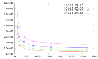
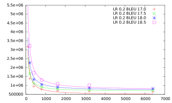
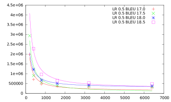
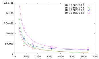
Figure 2: MT results are shown for learning rate, LR, equal to 0.1, 0.2, 0.5, and 1.0. For four learning error targets (i.e., MT BLEU scores), the measured $N$ values (y-axis) are plotted against their corresponding $M$ values (x-axis). The solid lines show that this data is well fit by the $N_{\rm{Update}}=N_{\infty}+\alpha/M$ model. Points are omitted where training did not achieve a specified BLEU score.

Theoretical Bound on $N_{\rm{Update}}$ for SGD

For completion, we provide a theoretical analysis of mini-batch SGD convergence that supports our finding of a robust empirical inverse relation between $N_{\rm{Update}}$ and $M$. We begin by defining the SGD update step as

$$w^{k+1}=w^{k}-\eta\left(\nabla f\left(w^{k}\right)+\xi^{k}\right)$$

where $f$ is the function to be optimized, $w^{k}$ is a vector of neural net weights at the $k^{\rm th}$ update of the SGD algorithm, $\xi^{k}$ is a zero-mean noise term with variance smaller than $\phi^{2}$, and $\eta$ is the SGD step size. We assume that $\nabla f$ is Lipschitz continuous, i.e., that

$$f\left(x\right)\leq f\left(y\right)+\nabla f\left(y\right)\cdot\left(x-y\right)+\frac{L}{2}\ \left|x-y\right|^{2}$$

for some constant $L$. Standard convex analysis steps along with $E[\xi^{k}]=0$ and Var$[\xi^{k}]\leq\phi^{2}$, gives

$$E_{\xi^{k}}\left[f\left(w^{k+1}\right)\right]\leq f\left(w^{k}\right)-\eta\left(1-\frac{\eta L}{2}\right)\left|\nabla f\left(w^{k}\right)\right|^{2}\ +\eta^{2}\frac{L}{2}\phi^{2}.$$

We define $\Delta_{k}$ to be the residual at the $k^{\rm th}$ step, i.e.,

$$\Delta_{k}\equiv f\left(w^{k}\right)-f\left(w^{*}\right)$$

where $w^{*}$ is the global minimum of $f$. Using the residual, assuming convexity, we get

$$\frac{\Delta_{k}}{|w^{0}-w^{*}|}\leq\frac{\Delta_{k}}{\left|w^{k}-w^{*}\right|}\leq\left|\nabla f\left(w^{k}\right)\right|.$$

Choosing the learning rate $\eta$ such that

$$\left(1-\frac{\eta L}{2}\right)>0$$

results in

$$E_{\xi^{k}}[\Delta_{k+1}]\leq\Delta_{k}-\lambda\Delta_{k}^{2}+\lambda\sigma^{2}$$

where

$$\lambda\equiv\eta\left(1-\frac{\eta L}{2}\right)\ \frac{1}{\left(w^{0}-w^{*}\right)^{2}}\text{~{}~{} and~{}~{} }\sigma^{2}\equiv\frac{\eta^{2}L}{2\lambda}\phi^{2}.$$

Now, we take average over the full history and use the fact that

$$(E[X])^{2}\leq E[X^{2}]$$

to obtain

$$E[\Delta_{k+1}]\leq E[\Delta_{k}]-\lambda(E[\Delta_{k}])^{2}+\lambda\sigma^{2}.$$

For simplicity from here forward, the expectation sign will be omitted by using $\Delta_{k}\equiv E_{\xi^{1}\xi^{2}\cdots\xi^{k-1}}[\Delta_{k}]$. We rearrange this inequality as

$$(\Delta_{k+1}-\sigma)\leq(\Delta_{k}-\sigma)(1-\lambda(\Delta_{k}+\sigma))$$

and observing that $\Delta_{k}$ cannot be smaller than $\sigma$ because of constant learning rate and additive noise, implies

$$1-\lambda\left(\Delta_{k}+\sigma\right)\geq 0.$$

By taking the inverse and using the fact that

$$\frac{1}{1-x}\geq 1+x\ \ \ \ {\rm for}\ \ \ \ x\leq 1$$

we obtain

$$\frac{1}{\Delta_{k+1}-\sigma}\geq\frac{1}{\Delta_{k}-\sigma}\left(\ 1+\lambda\left(\Delta_{k}+\ \sigma\right)\right)=\frac{1+2\lambda\sigma}{\Delta_{k}-\sigma}+\eta.$$

Then, telescoping this recurrence inequality results in

$$\frac{1}{\Delta_{k+1}-\sigma}+\frac{1}{2\sigma}\geq\left(1+2\lambda\sigma\right)^{k+1}\left(\frac{1}{\Delta_{0}-\sigma}+\frac{1}{2\sigma}\right).$$

Finally, solving for $\Delta_{k}$, gives

$$\Delta_{k}\leq\frac{1}{\left(1+2\lambda\sigma\right)^{k}\left(\frac{1}{\Delta_{0}-\sigma}+\frac{1}{2\sigma}\right)\ -\frac{1}{2\sigma}}+\sigma$$

and, Taylor expanding for small $\sigma$, the number of updates to reach $\Delta_{k}\leq\epsilon$ is given by

$$N_{\rm{Update}} \geq\frac{\log\left[\frac{\epsilon+\sigma}{\epsilon-\sigma}\right]+\log\left[\frac{\Delta_{0}-\sigma}{\Delta_{0}+\sigma}\right]}{\log\left[1+2\lambda\sigma\right]}$$

$$\approx\frac{1}{\lambda}\left(\frac{1}{\epsilon}-\frac{1}{\Delta_{0}}\right)\left(1+\frac{\sigma^{2}}{3}\left(\frac{1}{\epsilon^{2}}+\frac{1}{\Delta_{0}^{2}}+\frac{1}{\epsilon\Delta_{0}}\right)\right).$$

Using the Central Limit Theorem, we observe that $\sigma^{2}\approx\frac{\theta}{M}$ and therefore obtain

$$N_{\text{Update}}\geq\frac{1}{\lambda}\ \left(\frac{1}{\epsilon}-\frac{1}{\Delta_{0}}\right)\left(1+\frac{\theta}{M}\left(\frac{1}{\epsilon^{2}}+\frac{1}{\Delta_{0}^{2}}+\frac{1}{\epsilon\Delta_{0}}\right)\right).$$

The fact that this bound exhibits the same inverse $M$ relationship as

$$N_{\rm{Update}}=N_{\infty}+\frac{\alpha}{M}$$

reinforces the robustness of our empirical finding.

Discussion

Our model separates algorithmic convergence properties from implementation details. This separation provides machine learning researchers and practitioners a new way of thinking about their algorithms: $N_{\infty}$ provides a lower bound on the number of updates required to converge and fundamentally limits the benefits of parallelization for accelerating machine learning; and $\alpha$ introduces a new concept, that of an algorithm’s “noise sensitivity”, as a key property in the optimization of machine learning. Using these new principles to guide algorithmic design may help researchers develop improved algorithms.

We close with a few observations about challenges and opportunities ahead.

Noise Sensitivity and Complexity: Our experiments suggest that as the learning problem grows in complexity from MNIST to CIFAR10 to CIFAR100, its sensitivity to noise grows (i.e., $\alpha$ grows). See for example the medium size model results for fixed learning rate. Thus, the onset of the $N_{\infty}$ “floor” is pushed to larger mini-batch values. This suggests that the benefit of parallelism may grow as the research community explores more complex learning challenges. However, this benefit must be balanced by any related increase in $N_{\infty}$, which will in general also grow with complexity.

Improved Learning Algorithms: The research community should be encouraged to develop algorithms with lower $N_{\infty}$ as this will lead to better data-parallel scaling.

Beyond SGD: The core methodology presented in this paper is not limited to SGD. Research is required to explore whether other robust mini-batch (or other) relationships exist for different algorithms, such as Expectation Maximization (?). In this way, the methodology described in this paper provides a new way of comparing the parallelization effectiveness of algorithms.

References

- [Bahdanau et al., 2014] Bahdanau, D., Cho, K., and Bengio, Y. (2014). Neural machine translation by jointly learning to align and translate. CoRR, abs/1409.0473.
- [Bottou et al., 2018] Bottou, L., Curtis, F., and Nocedal, J. (2018). Optimization methods for large-scale machine learning. SIAM Review, 60(2):223–311.
- [Chetlur et al., 2014] Chetlur, S., Woolley, C., Vandermersch, P., Cohen, J., Tran, J., Catanzaro, B., and Shelhamer, E. (2014). cuDNN: Efficient primitives for deep learning. arXiv:1410.0759.
- [Cho et al., 2014] Cho, K., van Merrienboer, B., Bahdanau, D., and Bengio, Y. (2014). On the properties of neural machine translation: Encoder-decoder approaches. CoRR, abs/1409.1259.
- [Cho et al., 2017] Cho, M., Finkler, U., Kumar, S., Kung, D., Saxena, V., and Sreedhar, D. (2017). PowerAI DDL. arXiv:1708.02188.
- [Coates et al., 2013] Coates, A., Huval, B., Wang, T., Wu, D., Catanzaro, B., and Andrew, N. (2013). Deep learning with COTS HPC systems. In ICML, pages 1337–1345.
- [Cotter et al., 2011] Cotter, A., Shamir, O., Srebro, N., and Sridharan, K. (2011). Better mini-batch algorithms via accelerated gradient methods. In Advances in NIPS, pages 1647–1655.
- [Dean et al., 2012] Dean, J., Corrado, G., Monga, R., Chen, K., Devin, M., Mao, M., Senior, A., Tucker, P., Yang, K., and Le, Q. (2012). Large scale distributed deep networks. In Advances in NIPS, pages 1223–1231.
- [Dekel et al., 2012] Dekel, O., Gilad-Bachrach, R., Shamir, O., and Xiao, L. (2012). Optimal distributed online prediction using mini-batches. Journal of Machine Learning Research, 13(Jan):165–202.
- [Dempster et al., 1977] Dempster, A., Laird, N., and Rubin, D. (1977). Maximum likelihood from incomplete data via the EM algorithm. Journal of the royal statistical society. Series B, pages 1–38.
- [Goyal et al., 2017] Goyal, P., Dollár, P., Girshick, R., Noordhuis, P., Wesolowski, L., Kyrola, A., Tulloch, A., Jia, Y., and He, K. (2017). Accurate, large minibatch SGD: training imagenet in 1 hour. arXiv:1706.02677.
- [He et al., 2016] He, K., Zhang, X., Ren, S., and Sun, J. (2016). Deep residual learning for image recognition. In Proceedings of the IEEE conference on CVPR, pages 770–778.
- [Jain et al., 2017] Jain, P., Netrapalli, P., Kakade, S., Kidambi, R., and Sidford, A. (2017). Parallelizing stochastic gradient descent for least squares regression: mini-batching, averaging, and model misspecification. Journal of Machine Learning Research, 18(1):8258–8299.
- [Keskar et al., 2016] Keskar, N. S., Mudigere, D., Nocedal, J., Smelyanskiy, M., and Tang, P. (2016). On large-batch training for deep learning: Generalization gap and sharp minima. arXiv:1609.04836.
- [Kingma and Ba, 2014] Kingma, D. and Ba, J. (2014). Adam: A method for stochastic optimization. arXiv:1412.6980.
- [Koehn, 2005] Koehn, P. (2005). Europarl: A parallel corpus for statistical machine translation. In Conference Proceedings: the Tenth Machine Translation Summit, pages 79–86.
- [Krizhevsky, 2014] Krizhevsky, A. (2014). One weird trick for parallelizing convolutional neural networks. arXiv:1404.5997.
- [Kumar et al., 2016] Kumar, S., Sharkawi, S., and Jan, N. (2016). Optimization and analysis of MPI collective communication on fat-tree networks. In Parallel and Distributed Processing Symposium, pages 1031–1040. IEEE.
- [LeCun et al., 1995] LeCun, Y., Jackel, L., Bottou, L., Cortes, C., Denker, J., Drucker, H., Guyon, I., Muller, U., Sackinger, E., and Simard, P. (1995). Learning algorithms for classification: A comparison on handwritten digit recognition. Neural networks: the statistical mechanics perspective, 261:276.
- [Li et al., 2014a] Li, M., Andersen, D., Park, J. W., Smola, A., Ahmed, A., Josifovski, V., Long, J., Shekita, E., and Su, B.-Y. (2014a). Scaling distributed machine learning with the parameter server. In OSDI, volume 14, pages 583–598.
- [Li et al., 2014b] Li, M., Zhang, T., Chen, Y., and Smola, A. (2014b). Efficient mini-batch training for stochastic optimization. In Proceedings of the 20th ACM SIGKDD international conference, pages 661–670. ACM.
- [Lian et al., 2015] Lian, X., Huang, Y., Li, Y., and Liu, J. (2015). Asynchronous parallel stochastic gradient for nonconvex optimization. In Advances in NIPS, pages 2737–2745.
- [Paszke et al., 2017] Paszke, A., Gross, S., Chintala, S., Chanan, G., Yang, E., DeVito, Z., Lin, Z., Desmaison, A., Antiga, L., and Lerer, A. (2017). Automatic differentiation in pytorch. In NIPS-W.
- [Recht et al., 2011] Recht, B., Re, C., Wright, S., and Niu, F. (2011). Hogwild: A lock-free approach to parallelizing stochastic gradient descent. In Advances in NIPS, pages 693–701.
- [Seide et al., 2014] Seide, F., Fu, H., Droppo, J., Li, G., and Yu, D. (2014). On parallelizability of stochastic gradient descent for speech DNNs. In Acoustics, Speech and Signal Processing (ICASSP), pages 235–239. IEEE.
- [Sennrich et al., 2017] Sennrich, R., Firat, O., Cho, K., Birch, A., Haddow, B., Hitschler, J., Junczys-Dowmunt, M., Läubli, S., Miceli Barone, A. V., Mokry, J., and Nadejde, M. (2017). Nematus: a toolkit for neural machine translation. In Proceedings of the Software Demonstrations of the 15th Conference of the European Chapter of the Association for Computational Linguistics, pages 65–68.
- [Simonyan and Zisserman, 2014] Simonyan, K. and Zisserman, A. (2014). Very deep convolutional networks for large-scale image recognition. arXiv:1409.1556.
- [Tan et al., 2011] Tan, G., Li, L., Triechle, S., Phillips, E., Bao, Y., and Sun, N. (2011). Fast implementation of DGEMM on Fermi GPU. In Proceedings of 2011 International Conference for HPC, Networking, Storage and Analysis, page 35. ACM.
- [Watcharapichat et al., 2016] Watcharapichat, P., Morales, V. L., Fernandez, R. C., and Pietzuch, P. (2016). Ako: Decentralised deep learning with partial gradient exchange. In Proceedings of the Seventh ACM Symposium on Cloud Computing, pages 84–97. ACM.
- [Zhang et al., 2015] Zhang, S., Choromanska, A., and LeCun, Y. (2015). Deep learning with elastic averaging SGD. In Advances in NIPS, pages 685–693.