Modelling EHR timeseries by restricting feature interaction

Abstract

Time series data are prevalent in electronic health records, mostly in the form of physiological parameters such as vital signs and lab tests. The patterns of these values may be significant indicators of patients’ clinical states and there might be patterns that are unknown to clinicians but are highly predictive of some outcomes. Many of these values are also missing which makes it difficult to apply existing methods like decision trees. We propose a recurrent neural network model that reduces overfitting to noisy observations by limiting interactions between features. We analyze its performance on mortality, ICD-9 and AKI prediction from observational values on the Medical Information Mart for Intensive Care III (MIMIC-III) dataset. Our models result in an improvement of 1.1% [p<0.01] in AU-ROC for mortality prediction under the MetaVision subset and 1.0% and 2.2% [p<0.01] respectively for mortality and AKI under the full MIMIC-III dataset compared to existing state-of-the-art interpolation, embedding and decay-based recurrent models.

1 Introduction

Observational values, such as lab results and vital signs, are frequently used to make a quantitative estimation of the current physiological state of a patient. However, these values are mostly processed into pre-specified ranges and buckets. For example, when calculating the commonly-used Acute Physiology and Chronic Health Evaluation (APACHE) IV score [1], there are as few as 3 buckets for some of the physiological measurements of the patients. These buckets have been assumed to be equally representative for all patients and ignore patients’ different healthy baseline values. In addition, these score systems also ignore how the lab values are changing. For example, a systolic blood pressure that was rapidly trending from 111 to 219 would give the same NEWS score contribution of 0, although for many clinicians this would be an adverse indicator. These trend signals and many others are lost with many of the existing methods of processing lab values.

Predictive models such as mortality or billing code prediction utilise lab values, vital signs and other measurements to improve predictive accuracy. However, missing values are prevalent in EHR data since lab tests are ordered at the physician’s discretion and costly or impractical measurements are not taken unless necessary. This results in time series data where the patterns of missingness can be predictive of risk or a diagnosis [2]. For the modelling of time series data, observational values are typically standardized, while missing values are carried forward, interpolated from the previous value or are modelled to decay to the population mean [3]. The patterns of missingness are typically represented as binary missingness indicator variables.

Recently, recurrent neural networks (RNNs) have been applied to electronic health records for more accurate clinical predictions [4]. Overfitting is a common problem for deep learning models. Deep learning models are often overparameterized and so it is easy for the model to memorize the training data while failing to generalize to unseen data.

We introduce the feature-grouped long short-term memory network (FG-LSTM) that operates by modelling features individually and limiting their interactions in the model. The FG-LSTM specializes the long short-term memory network (LSTM [5]) by restricting the form of the weight matrices. To ensure that missingness and time gaps are modelled, we represent each input feature (such as creatinine) by a group of two or three input variables: the standardized measurement value (interpolated if missing), a binary variable indicating presence or absence and an optional variable indicating the time since the feature was last measured. For a given input feature, the FG-LSTM allows all these components to interact but prevents features from interacting with each other. This reduces overfitting in the model and prevents learning spurious interactions or correlations between certain features over a few short timesteps. At inference time, features can only interact after each entire sequence of features has been read, which tends to produce smoother predictions over time.

2 Methods

In the FG-LSTM, each input feature is represented by a group of two or three variables (referred to as a feature group). We denote a multivariate time series indexed by $t$ as a vector $x_{t}=(u_{t},v_{t},w_{t})$ where $u_{t}=(u_{1t},\ldots,u_{pt})$ denote the standardized values for the $p$ features, $v_{t}=(v_{1t},\ldots,v_{pt})$ denote the binary missing indicators where 0 indicates a feature is missing and $w_{t}=(w_{1t},\ldots,w_{pt})$ optionally denote the time since the last observation. The standardized value is linearly interpolated between adjacent values when it is missing (taking time into account), and simply carried forward when all future values are missing as in the interpolation baseline. The time differences are defined similarly to GRU-D where $s_{t}$ is the absolute time when the $t$^th observation was obtained (after windowing) and $s_{1}$ is set to 0. The time differences are normalised to be between 0 and 1.

$$w_{kt}=\begin{cases}s_{t}-s_{t-1}+w_{kt-1},&t>1,v_{kt-1}=0\\ s_{t}-s_{t-1},&t>1,v_{kt-1}=1\\ 0,&t=1\end{cases}$$ (1)

When the time differences are not used, the vector only consists of $u$ and $v$. $x_{t}$ represents the set of observations at timestep $t$. A naive setup would be to run $p$ small recurrent neural networks, one for each feature group, but running many small RNNs can potentially be inefficient due to not being able to use a single large matrix multiplication. Instead, we feed all $p$ feature groups into a single RNN where constrained weight matrices are used to restrict feature interaction. We describe this as a FG-LSTM (feature grouped long short-term memory network). We define FG-LSTM by the following equations (which are a variant of the LSTM equations):

$$f_{t} =\sigma((W_{f}\cdot M_{w})x_{t}+(U_{f}\cdot M_{u})h_{t-1}+b_{f})$$ (2)

$$i_{t} =\sigma((W_{i}\cdot M_{w})x_{t}+(U_{i}\cdot M_{u})h_{t-1}+b_{i})$$ (3)

$$o_{t} =\sigma((W_{o}\cdot M_{w})x_{t}+(U_{o}\cdot M_{u})h_{t-1}+b_{o})$$ (4)

$$c_{t} =f_{t}\cdot c_{t-1}+i_{t}\cdot\tanh((W_{c}\cdot M_{w})x_{t}+(U_{c}\cdot M_{u})h_{t-1}+b_{c})\qquad h_{t}=o_{t}\cdot\tanh(c_{t})$$ (5)

Here, $\sigma$ denotes the sigmoid function, $\tanh$ denotes the hyperbolic tangent function, and $\cdot$ denotes the Hadamard (elementwise) product. The weights $W_{\{f,i,o,c\}}$, $U_{\{f,i,o,c\}}$ and bias terms $b_{\{f,i,o,c\}}$ are learned during training. $M_{w}$ is a fixed binary mask for the input-to-hidden weight matrices, and $M_{u}$ is a fixed binary mask for the hidden-to-hidden weight matrices. The effect of the mask is to restrict the weight matrix so that each element of the hidden state and cell state of the LSTM is computed from only one feature group. The mask is defined as follows.

$$M_{wij}=\begin{cases}1&\text{if }i\mod p=j\mod p\\ 0&\text{otherwise}\end{cases}$$ (6)

$M_{u}$ is defined similarly. The FG-LSTM can be considered similar to running $p$ individual LSTM models. The hidden state of the LSTM at the last timestep of the sequence is passed through a dense fully-connected layer to generate predictions. Only at this point are the activations of the layer computed from multiple features so that they can interact. A sigmoid or softmax activation is then applied depending on the task (sigmoid for binary (AKI/mortality), softmax for ICD-9). The model is trained to minimize the cross-entropy loss on the ground-truth labels. Models were optimized using AdaGrad [6] or Adam [7] depending on the model. Standard dropout techniques were applied to models including standard input and hidden-layer dropout[8], variational input and hidden-layer dropout[9], and zoneout[10].

For the baselines, we use the author provided Keras implementation of GRU-D, as well as standard median and linear interpolation. We have also reported the performance of FG-LSTM with and without the time difference. In all experiments, 80%, 10% and 10% of patients were used as the train, validation and test sets respectively randomly split based on patient ID. The validation set was used for model hyperparameter tuning for FG-LSTM and all the baselines through Gaussian process bandit hyperparameter optimization [11]. The hyperparameter limits are listed in Table S6 with the final tuned hyperparameters listed in Table S7. All models were implemented in TensorFlow [12].

3 Dataset

We conduct experiments on the MIMIC-III dataset [13], a publicly available dataset of critical care records. Each patient’s medical data during the first 48 hours in the current hospitalization is represented as a time series as described in Rajkomar et al. [4].

Our cohort consists of inpatients hospitalized for at least 48 hours. We require the patient’s age to be greater or equal to 18 years at the time of admission. We present results on the full cohort as well as MetaVision and CareVue subsets of the cohort which contain significantly different data as described in Mark [14]. The MetaVision cohort is the same cohort as used in Che et al. [3], which has been claimed to be superior quality data. The test cohort is described in Table LABEL:tab:test-cohort.

We use the top 100 observational features according to measurement frequency as predictor features; these are listed in Table LABEL:tab:features. Each feature is standardized (transformed to have a median of 0 and standard deviation of 1) according to training set statistics.

Measurements are grouped into 20-minute windows, and we take the average if there are multiple measurements in the same window. A time step is skipped in the sequence if no features are present in that window. Outliers are handled by clipping the value to 10 standard deviations.

4 Experiments

The following outcomes are predicted for each patient using the predictor variables described above. All predictions are at 48 hours after admission. More details are in the appendix.

Mortality: Whether the patient dies during the current hospital admission.

AKI: Predicting acute kidney injury (AKI) onset within the inpatient encounter.

ICD-9 20 task classification: The ICD-9 diagnosis codes are grouped into 20 categories following Che et al. [3] .

We report results with our model (FG-LSTM) along with several baselines. All baselines concatenate the input with a missingness indicator for each feature (unless mentioned) and use a LSTM model (unless specified). Outliers are handled by clipping the value to 10 standard deviations. Our preliminary experiments indicate that these outliers carry information and that removing them from the data results in a loss of performance. The baselines we use are described in detail in the appendix.

We report the test-set performance over 5 runs using the best validation set hyperparameters from different random initializations. We report both the area under the receiver operating characteristic curve (AU-ROC) and the area under the precision recall curve (AU-PRC).

Table 2 compares the performance of our model (FG-LSTM) with several state of the art baselines on the full MIMIC-III dataset. The FG-LSTM results in significant absolute increases in AU-ROC of 1.0% (Welch’s t-test: P<0.001) and 2.2% (Welch’s t-test: P<0.0001) respectively for mortality and AKI compared to the best baseline models (interpolation and GRU-D). For the task of ICD-9 20 task classification we find our model’s results are not significantly different from that of the GRU-D. We find that for ICD9 20 task classification, using the time differences improves performance, whereas there is no significant impact for mortality and AKI classification. We show the results of further ablations with FG-LSTM in Table S8.

Table 1: Results on patient mortality, AKI and ICD-9 20 task classification at 48 hours after admission on the MIMIC-III dataset. We report the mean (standard deviation) for each metric over five repeated runs. We also report the significance of the difference between the FG-LSTM results and the best baseline model under Welch’s t-test, where applicable.

	Mortality		AKI
	AU-ROC	AU-PRC	AU-ROC	AU-PRC
Percentile embedding w/o indicator	0.8344 (0.0015)	0.3456 (0.0081)	0.7159 (0.0058)	0.4297 (0.0095)
Percentile embedding	0.8371 (0.0024)	0.3437 (0.0062)	0.7205 (0.0050)	0.4365 (0.0054)
Median	0.8399 (0.0021)	0.3864 (0.0094)	0.7316 (0.0031)	0.4501 (0.0070)
Interpolation	0.8564 (0.0032)	0.4009 (0.0122)	0.7433 (0.0021)	0.4630 (0.0047)
GRU-D	0.8544 (0.0033)	0.4195 (0.0084)	0.7474 (0.0025)	0.4688 (0.0050)
FG-LSTM	0.8665 (0.0020)***	0.4225 (0.0065)	0.7689 (0.0023)***	0.4785 (0.0036)**
FG-LSTM w/ time differences	0.8630 (0.0030)	0.4126 (0.0033)	0.7489 (0.0022)	0.4679 (0.0055)
	ICD-9 20 task classification
Percentile embedding w/o indicator	0.8444 (0.0004)	0.7408 (0.0005)
Percentile embedding	0.8465 (0.0006)	0.7450 (0.0009)
Median	0.8495 (0.0003)	0.7515 (0.0005)
Interpolation	0.8492 (0.0004)	0.7500 (0.0004)
GRU-D	0.8489 (0.0004)	0.7506 (0.0008)
FG-LSTM	0.8488 (0.0003)	0.7500 (0.0003)
FG-LSTM w/ time differences	0.8496 (0.0003)	0.7511 (0.0005)

Table 2: *

**p < 0.01 ***p < 0.001

We also conducted experiments on admissions restricted to patients monitored using the MetaVision system in MIMIC-III. This is similar to the cohort from the GRU-D paper [3]. Table S2 compares the performance of FG-LSTM and the baselines trained and tested under the MetaVision subset of the dataset, which is claimed by Che et al. [3] to be superior quality in terms of time series data. We see a drop in performance on this subset, likely because it is only a third of the size of the full dataset. The FG-LSTM results in a significant absolute improvement of 1.1% (Welch’s t-test: P=0.0081) in AU-ROC for mortality under this MetaVision subset. Again for the task of ICD-9 20 task classification, there is no significant difference from GRU-D.

5 Discussion

Our results show that the FG-LSTM performs significantly (under Welch’s t-test) better than the state-of-the-art baseline methods (GRU-D and linear feature interpolation) for mortality and AKI prediction. These tasks are particularly sensitive to vital signs and lab values so it’s reasonable that the FG-LSTM models these well. The insignificant results on ICD-9 20 class prediction is likely because the input features we chose were not significantly predictive of different diagnoses and it is possible that the other categorical or notes data in the EHR are better predictors for this task. In the appendix, we show that the FG-LSTM also yields more interpretable attribution than the baseline models. For future work, we expect the combination of the FG-LSTM with a model that handles categorical features as in Rajkomar et al. [4] can lead to better predictions for diagnosis, mortality and AKI.

Appendix

Table S1: Results on patient mortality and the ICD-9 20 task at 48 hours after admission after training and testing on the MetaVision subset of MIMIC-III.

	Mortality		ICD-9 20 task classification
	AU-ROC	AU-PRC	AU-ROC	AU-PRC
Percentile embedding w/o indicator	0.8218 (0.0038)	0.2903 (0.0030)	0.8384 (0.0007)	0.7726 (0.0012)
Percentile embedding	0.8378 (0.0058)	0.3267 (0.0068)	0.8374 (0.0007)	0.7716 (0.0011)
Median	0.8417 (0.0043)	0.3677 (0.0176)	0.8379 (0.0005)	0.7727 (0.0008)
Interpolation	0.8373 (0.0099)	0.3473 (0.0267)	0.8402 (0.0003)	0.7762 (0.0003)
GRU-D	0.8484 (0.0037)	0.3856 (0.0057)	0.8410 (0.0005)	0.7787 (0.0007)
FG-LSTM	0.8591 (0.0054)**	0.3757 (0.0101)	0.8419 (0.0002)	0.7796 (0.0003)
FG-LSTM w/ time differences	0.8567 (0.0019)	0.3813 (0.0087)	0.8420 (0.0005)	0.7793 (0.0005)

Table S2: *

**p < 0.01

Task details

The following outcomes are predicted for each patient using the predictor variables described above.

Mortality

Whether the patient dies during the current hospital admission. Predicted at 48 hours after admission. The dataset contains 46,120 admission records from 35,440 patients, with 4,277 positive labels.

AKI

Predicting acute kidney injury (AKI) onset within the inpatient encounter at 48 hours after admission. This dataset contains 46,120 records from 35,440 patients, and has 10,180 positive labels.

AKI is a sudden episode of kidney failure or kidney damage that happens within a few hours or a few days. It is a common complication among hospitalized patients, and is an important cause for in-hospital death. Multiple criteria exist for AKI diagnosis. We adopt the KDIGO (Kidney Disease Improving Global Organization) criteria based on short-term lab value changes in our prediction tasks here:

• Increase in serum creatinine by $\geq$ 0.3 mg/dl ($\geq$ 26.5 umol/l) within 48 hours;

• Urine volume < 0.5 ml/kg/h (25ml/h, assuming 50kg weight) for 6 hours.

At 48 hours after admission, we classify the patients who have not developed AKI but will have AKI within this encounter as positive and the others as negative examples.

ICD-9 20 task classification

The ICD-9 diagnosis codes are grouped into 20 categories following Che et al. [3] . This is then predicted at 48 hours after admission, which has a total of 46,120 admission records from 35,440 patients.

Baselines

Percentile embedding w/o indicator

Features are bucketed by percentiles and then the buckets are embedded, where each bucket embedding is initialized to a random vector and trained jointly. Any missing values are ignored. The number of buckets is tuned on the validation set. This is the method as described in the deep models in Rajkomar et al. [4].

Percentile embedding

As in the model above but the embedding vector is concatenated with a missingness indicator for each feature.

Median

Standardized feature values are used and missing values are filled in with the median from the training set.

Interpolation

Standardized feature values are used and linear interpolation is used to fill in the missing values. To interpolate a missing value $v$ at time $t$ between 2 measurements $v_{1}$ measured at $t_{1}$ and $v_{2}$ measured at $t_{2}$, $v=v_{1}+(v_{2}-v_{1})\frac{t-t_{1}}{t_{2}-t_{1}}$. If there is no measurement after $v_{1}$, the value $v_{1}$ is simply carried forward. If there is no measurement before $v_{2}$, the value $v_{2}$ is carried backward. If there is no measurement during the period, 0 will be used.

GRU-D

The GRU based model as implemented by Che et al. [3] in TensorFlow which has trainable decay rates for the input and hidden states.

Attribution Methods

Deep learning techniques are typically regarded as black boxes where it is hard to determine what causes a model to make a prediction. Recent advances in interpretability techniques have produced better tools to probe a trained model. One of these is path-integrated gradients [15]. Gradients can be used to approximate the change in a prediction given a step change in the input data. Path-integrated gradients have been shown to produce a better approximation of the change in a prediction by summing gradients over a gradual change in the input data. This has typically been applied to images but here we adapt it to time series data.

To apply this technique to sparsely measured time series for a particular patient, we use as a baseline a patient who has had the same measurements recorded at the same times, but for whom all measurements take the population median value. We then average the gradients of the model prediction across 50 evenly-spaced points between this baseline and the actual measurements. For each lab and measurement time, we take the product of this averaged gradient with the change from measurement to baseline value as a linearized approximation of the influence of that value on the generated prediction. Because the population median is mapped to zero in our normalization, we can represent the contribution of each lab type and time of measurement simply. If $F(x)$ is the neural network’s predicted probability of an event, as a function of the first 48 hours of lab values, then:

$$\textrm{IntGrad}(x_{it})=\frac{x_{it}}{50}\sum_{k=1}^{50}\frac{\partial F(kx/50)}{\partial x_{it}}$$ (7)

Dataset details

Table S3: Descriptive statistics for patient cohort. These consist of inpatients who are admitted for at least 48 hours in the MIMIC-III dataset and are used for training or validation purposes.

Demographics	Adult MIMIC admissions		MetaVision Only (GRU-D cohort)
Number of Patients	31,786		14,467
Number of Encounters	41,387		17,777
Number of Female Patients	18,210	44.2%	7,874	44.3%
Median Age (Interquartile Range)	66	(25)	66	(24)
Disease Cohort
Cancer	2,978	7.2%	1,359	7.6%
Cardiopulmonary	4,279	10.3%	1,924	10.8%
Cardiovascular	10,515	25.4%	3,715	20.9%
Medical	17,862	43.2%	8,409	47.3%
Neurology	4,998	12.1%	2,218	12.5%
Obstetrics	131	0.3%	47	0.3%
Psychiatric	28	0.1%	18	0.1%
Other	596	1.4%	87	0.5%
Number of Previous Hospitalizations
0	31,463	76.0%	12,874	72.4%
1	5,932	14.3%	2,725	15.3%
2-5	3,429	8.3%	1,845	10.4%
6+	563	1.4%	333	1.9%
Discharge Disposition
Expired	3,858	9.3%	1,520	8.6%
Home	21,022	50.8%	8,876	49.9%
Other	1,079	2.6%	599	3.4%
Other Healthcare Facility	2,938	7.1%	1,809	10.2%
Rehabilitation	5,706	13.8%	1,657	9.3%
Skilled Nursing Facility	6,784	16.4%	3,316	18.7%
Binary Label Prevalence
Mortality	3,858	9.3%	1,520	8.6%
Acute Kidney Injury (AKI)	9,110	22.0%
Multilabel Prevalence (ICD9 Groups)
1:Infectious and Parasitic Diseases	11,632	28.1%	5,827	32.8%
2:Neoplasms	7,293	17.6%	3,651	20.5%
3:Endocrine, Nutritional and Metabolic Diseases, Immunity	28,749	69.5%	13,929	78.4%
4:Blood and Blood-Forming Organs	15,732	38.0%	8,340	46.9%
5:Mental Disorders	13,232	32.0%	7,558	42.5%
6:Nervous System and Sense Organs	12,913	31.2%	8,004	45.0%
7:Circulatory System	34,985	84.5%	15,327	86.2%
8:Respiratory System	20,422	49.3%	9,379	52.8%
9:Digestive System	17,289	41.8%	8,735	49.1%
10:Genitourinary System	17,947	43.4%	9,066	51.0%
11:Complications of Pregnancy, Childbirth, and the Puerperium	142	0.3%	52	0.3%
12:Skin and Subcutaneous Tissue	4,852	11.7%	2,494	14.0%
13:Musculoskeletal System and Connective Tissue	8,349	20.2%	4,929	27.7%
14:Congenital Anomalies	1,442	3.5%	725	4.1%
15:Symptoms	12,979	31.4%	7,506	42.2%
16:Nonspecific Abnormal Findings	3,786	9.2%	2,176	12.2%
17:Ill-defined and Unknown Causes of Morbidity and Mortality	1,364	3.3%	955	5.4%
18:Injury and Poisoning	18,211	44.0%	8,044	45.2%
19:Supplemental V-Codes	21,607	52.2%	12,001	67.5%
20:Supplemental E-Codes	13,512	32.7%	7,608	42.8%

Results on MIMIC-III CareVue subset

We also took the model trained on the full MIMIC-III cohort and analysed results solely on the CareVue subset (the records not in the MetaVision cohort) to determine if the quality of data affected the relative performance of the models.

Table S5 compares the performance of FG-LSTM and the baselines under the CareVue subset of the dataset, which are not considered by Che et al. [3] as they claim the data is worse quality. Again, for this subset we see a significant improvement in performance in mortality and AKI prediction using the FG-LSTM model as compared to the baselines. Again for the task of ICD-9 20 task classification, there is no significant difference from GRU-D. Interestingly, this shows that the poorer quality data does not affect the relative performance of the model.

Table S4: Results on patient mortality, AKI and ICD-9 20 task at 48 hours after admission on the CareVue subset of MIMIC-III.

	Mortality		AKI
	AU-ROC	AU-PRC	AU-ROC	AU-PRC
Percentile embedding w/o indicator	0.8280 (0.0027)	0.3456 (0.0094)	0.7078 (0.0063)	0.4250 (0.0099)
Percentile embedding	0.8298 (0.0024)	0.3488 (0.0036)	0.7152 (0.0052)	0.4371 (0.0040)
Median	0.8318 (0.0044)	0.3878 (0.0102)	0.7243 (0.0051)	0.4472 (0.0077)
Interpolation	0.8516 (0.0025)	0.4090 (0.0118)	0.7407 (0.0010)	0.4675 (0.0038)
GRU-D	0.8560 (0.0032)	0.4380 (0.0084)	0.7417 (0.0019)	0.4656 (0.0034)
FG-LSTM	0.8659 (0.0016)***	0.4362 (0.0111)	0.7691 (0.0023)***	0.4843 (0.0048)***
FG-LSTM w/ time differences	0.8620 (0.0020)	0.4251 (0.0076)	0.7445 (0.0046)	0.4683 (0.0078)
	ICD-9 20 task classification
Percentile embedding w/o indicator	0.8441 (0.0006)	0.7068 (0.0011)
Percentile embedding	0.8463 (0.0006)	0.7124 (0.0010)
Median	0.8497 (0.0003)	0.7195 (0.0003)
Interpolation	0.8503 (0.0005)	0.7202 (0.0006)
GRU-D	0.8495 (0.0004)	0.7194 (0.0010)
FG-LSTM	0.8499 (0.0005)	0.7197 (0.0008)
FG-LSTM w/ time differences	0.8510 (0.0005)	0.7208 (0.0010)

Table S5: *

***p < 0.001

Attribution

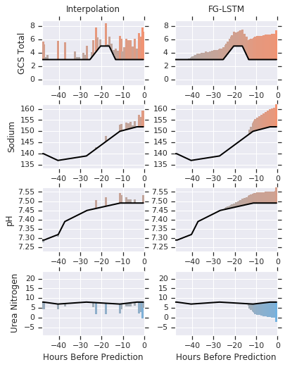
Figure 1: We show 4 features that contribute to the FG-LSTM’s prediction (right) in a different way than to the baseline interpolation model (left) via attribution, and their values for the preceding 48 hours prior to the prediction. The red-overlays indicate that the particular value had a positive attribution to the predicted risk for that model and the height of the red columns are proportional to the log-scaled attribution weight. The blue overlays indicate a negative attribution, which indicate a negative contribution to predicted risk for that model from that feature. GCS is the Glascow Coma Scale.

Figure 1 shows attribution over time for a particular patient to the four lab measurements with the biggest difference in attribution between the interpolation model and the FG-LSTM. The patient had a persistently low Glascow Coma Score (GCS) for the 48 hours preceding the prediction, which indicates that the patient had poor neurological function. The sodium and pH values indicate progressive hypernatremia and alkalosis, which are clinically considered to represent a worsening physiological state. The blood urea nitrogen level remained constant, which clinically correlates with stable kidney functions. The FG-LSTM and interpolation model have directionally similar attributions (in line with clinical expectations), but FG-LSTM’s attributions are more stable and smooth whereas the interpolation model has abrupt jumps in attribution despite small or no changes in the feature value. This is likely due to the interpolation model being overly sensitive to combinations of feature values over short periods of time. This can result in abrupt changes to predicted risk as measurements come in to the interpolation model as compared to the FG-LSTM.

Model Selection

We tuned the models with the following hyperparameters, targeting AU-ROC on the full MIMIC-III dataset. For the LSTM based models, the AdaGrad optimizer was used, for the GRU-D model, the Adam optimizer was used with batchnorm as in the paper. For the regularization techniques used, i.e. input dropout, LSTM hidden state dropout, projection layer dropout, zoneout, and variational dropout, we use $P_{k}$ to denote keep probability, which is 1 - dropout probability.

Table S6: Hyperparameter tuning limits used.

Hyperparameter	Minimum	Maximum
Clip norm	0.1	50.0
Input dropout $P_{k}$	0.01	1.0
RNN Hidden dropout $P_{k}$	0.01	1.0
Learning rate	0.0001	0.5
Percentile embedding size	25	200
Number of percentile buckets	5	20
RNN hidden size	16	3000
RNN hidden size per feature group	1	30
Projection layer dropout $P_{k}$	0.01	1.0
Projection layer size	0	1000
Variational input $P_{k}$	0.01	1.0
Variational output $P_{k}$	0.01	1.0
Variational recurrent $P_{k}$	0.01	1.0
Zoneout $P_{k}$	0.01	1.0

Table S7: Tuned hyperparameters found through Gaussian process bandit optimization.

Hyperparameter	Median	Percentile embedding	Interpolation	GRU-D	FG-LSTM
Clip norm	46.9164	48.9696	8.06007	32.90225	42.327009
Input dropout $P_{k}$	0.487627	0.326633	0.668343	0.747041	0.982881
RNN Hidden dropout $P_{k}$	0.854115	0.701658	0.88545	0.976599	0.356855
Learning rate	0.124912	0.19047	0.135474	0.001279	0.051977
Percentile embedding size	N/A	126	N/A	N/A	N/A
Number of percentile buckets	N/A	4	N/A	N/A	N/A
RNN hidden size	114	73	309	187	N/A
RNN hidden size per feature group	N/A	N/A	N/A	N/A	21
Projection layer dropout $P_{k}$	0.888716	0.874535	0.973923	0.987385	0.992444
Projection layer size	380	274	951	191	477
Variational input $P_{k}$	0.951351	0.491936	0.992106	N/A	N/A
Variational output $P_{k}$	0.990069	0.980551	0.856734	N/A	N/A
Variational recurrent $P_{k}$	0.974393	0.979701	0.643025	0.970241	0.986196
Zoneout $P_{k}$	0.358289	0.989134	0.748179	N/A	0.582535

Model ablation

We also conducted a few ablation experiments on the FG-LSTM on the mortality task.

W/o indicator

missingness indicators are removed from input.

W/o interpolation

missing values are filled with the median instead of interpolation.

All ablation experiments showed a significant drop of performance.

Table S8: FG-LSTM model ablation experiments results on mortality dataset. We report the mean (standard deviation) for each metric over five repeated runs.

	AU-ROC	AU-PRC
Full FG-LSTM	0.8665 (0.0020)	0.4225 (0.0065)
w/o indicator	0.8576 (0.0020)	0.4215 (0.0044)
w/o interpolation	0.8494 (0.0032)	0.3724 (0.0022)
w/o indicator and w/o interpolation	0.8420 (0.0010)	0.3674 (0.0087)

Table S9: Kernel size (total size of $W_{\{f,i,o,c\}},U_{\{f,i,o,c\}}$) comparison between the baseline interpolation model and the proposed FG-LSTM model.

Hidden state size	Corresponding FG-LSTM Per feature group state size	Size of baseline LSTM kernel	Effective Size of FG-LSTM kernel
50	–	50,000	–
100	1	120,000	1,200
200	2	320,000	3,200
300	3	600,000	6,000
400	4	960,000	9,600
500	5	1,400,000	14,000
1000	10	4,800,000	48,000
1500	15	10,200,000	102,000
2000	20	17,600,000	176,000

Table S10: Descriptive statistics for patient cohort in test set.

Demographics	Adult MIMIC admissions		MetaVision Only (GRU-D cohort)
Number of Patients	3,654		1,655
Number of Encounters	4,733		2,042
Number of Female Patients	1,970	41.6%	872	42.7%
Median Age (Interquartile Range)	66	(24)	66	(25)
Disease Cohort
Cancer	337	7.1%	149	7.3%
Cardiopulmonary	508	10.7%	218	10.7%
Cardiovascular	1260	26.6%	472	23.1%
Medical	2021	42.7%	964	47.2%
Neurology	545	11.5%	222	10.9%
Obstetrics	9	0.2%	4	0.2%
Psychiatric
Other	53	1.1%	13	0.6%
Number of Previous Hospitalizations
0	3622	76.5%	1471	72.0%
1	643	13.6%	302	14.8%
2-5	398	8.4%	221	10.8%
6+	70	1.5%	48	2.4%
Discharge Disposition
Expired	419	8.9%	159	7.8%
Home	2424	51.2%	1027	50.3%
Other	120	2.5%	70	3.4%
Other Healthcare Facility	341	7.2%	219	10.7%
Rehabilitation	649	13.7%	189	9.3%
Skilled Nursing Facility	780	16.5%	378	18.5%
Binary Label Prevalence
Mortality	419	8.9%	159	7.8%
Acute Kidney Injury (AKI)	1070	22.6%
Multilabel Prevalence (ICD9 Groups)
1:Infectious and Parasitic Diseases	1347	28.5%	647	31.7%
2:Neoplasms	806	17.0%	407	19.9%
3:Endocrine, Nutritional and Metabolic Diseases, Immunity	3288	69.5%	1593	78.0%
4:Blood and Blood-Forming Organs	1837	38.8%	965	47.3%
5:Mental Disorders	1513	32.0%	854	41.8%
6:Nervous System and Sense Organs	1408	29.8%	878	43.0%
7:Circulatory System	4026	85.0%	1764	86.4%
8:Respiratory System	2338	49.4%	1036	50.7%
9:Digestive System	1964	41.5%	985	48.2%
10:Genitourinary System	2061	43.6%	1069	52.4%
11:Complications of Pregnancy, Childbirth, and the Puerperium	12	0.3%	4	0.2%
12:Skin and Subcutaneous Tissue	574	12.1%	285	14.0%
13:Musculoskeletal System and Connective Tissue	1009	21.3%	594	29.1%
14:Congenital Anomalies	157	3.3%	87	4.3%
15:Symptoms	1385	29.3%	786	38.5%
16:Nonspecific Abnormal Findings	421	8.9%	250	12.2%
17:Ill-defined and Unknown Causes of Morbidity and Mortality	156	3.3%	115	5.6%
18:Injury and Poisoning	2047	43.3%	891	43.6%
19:Supplemental V-Codes	2475	52.3%	1391	68.1%
20:Supplemental E-Codes	1517	32.1%	869	42.6%

Table S11: List of input features used in the model.

Index	Observation Name	LOINC code	MIMIC specific code	Units
0	Heart Rate		211	bpm
1	SpO2		646	percent
2	Respiratory Rate		618	bpm
3	Heart Rate		220045	bpm
4	Respiratory Rate		220210	breaths per min
5	O2 saturation pulseoxymetry		220277	percent
6	Arterial BP [Systolic]		51	mmhg
7	Arterial BP [Diastolic]		8368	mmhg
8	Arterial BP Mean		52	mmhg
9	Urine Out Foley		40055	ml
10	HR Alarm [High]		8549	bpm
11	HR Alarm [Low]		5815	bpm
12	SpO2 Alarm [Low]		5820	percent
13	SpO2 Alarm [High]		8554	percent
14	Resp Alarm [High]		8553	bpm
15	Resp Alarm [Low]		5819	bpm
16	SaO2		834	percent
17	HR Alarm [Low]		3450	bpm
18	HR Alarm [High]		8518	bpm
19	Resp Rate		3603	breaths
20	SaO2 Alarm [Low]		3609	cm h2o
21	SaO2 Alarm [High]		8532	cm h2o
22	Previous WeightF		581	kg
23	NBP [Systolic]		455	mmhg
24	NBP [Diastolic]		8441	mmhg
25	NBP Mean		456	mmhg
26	NBP Alarm [Low]		5817	mmhg
27	NBP Alarm [High]		8551	mmhg
28	Non Invasive Blood Pressure mean		220181	mmhg
29	Non Invasive Blood Pressure systolic		220179	mmhg
30	Non Invasive Blood Pressure diastolic		220180	mmhg
31	Foley		226559	ml
32	CVP		113	mmhg
33	Arterial Blood Pressure mean		220052	mmhg
34	Arterial Blood Pressure systolic		220050	mmhg
35	Arterial Blood Pressure diastolic		220051	mmhg
36	ABP Alarm [Low]		5813	mmhg
37	ABP Alarm [High]		8547	mmhg
38	GCS Total		198	missing
39	Hematocrit	4544-3		percent
40	Potassium	2823-3		meq per l
41	Hemoglobin [Mass/volume] in Blood	718-7		g per dl
42	Sodium	2951-2		meq per l
43	Creatinine	2160-0		mg per dl
44	Chloride	2075-0		meq per l
45	Urea Nitrogen	3094-0		mg per dl
46	Bicarbonate	1963-8		meq per l
47	Platelet Count	777-3		k per ul
48	Anion Gap	1863-0		meq per l
49	Temperature F		678	deg f
50	Temperature C (calc)		677	deg f
51	Leukocytes [#/volume] in Blood by Manual count	804-5		k per ul
52	Glucose	2345-7		mg per dl
53	Erythrocyte mean corpuscular hemoglobin concentration [Mass/volume] by Automated count	786-4		percent
54	Erythrocyte mean corpuscular hemoglobin [Entitic mass] by Automated count	785-6		pg
55	Erythrocytes [#/volume] in Blood by Automated count	789-8		per nl
56	Erythrocyte mean corpuscular volume [Entitic volume] by Automated count	787-2		fl
57	Erythrocyte distribution width [Ratio] by Automated count	788-0		percent
58	Temp/Iso/Warmer [Temperature degrees C]		8537	deg f
59	FIO2		3420	percent
60	Magnesium	2601-3		mg per dl
61	CVP Alarm [High]		8548	mmhg
62	CVP Alarm [Low]		5814	mmhg
63	Calcium [Moles/volume] in Serum or Plasma	2000-8		mg per dl
64	Phosphate	2777-1		mg per dl
65	FiO2 Set		190	torr
66	Temp Skin [C]		3655	in
67	pH	11558-4		u
68	Temperature Fahrenheit		223761	deg f
69	Central Venous Pressure		220074	mmhg
70	Inspired O2 Fraction		223835	percent
71	PAP [Systolic]		492	mmhg
72	PAP [Diastolic]		8448	mmhg
73	Calculated Total CO2	34728-6		meq per l
74	Oxygen [Partial pressure] in Blood	11556-8		mmhg
75	Base Excess	11555-0		meq per l
76	Carbon dioxide [Partial pressure] in Blood	11557-6		mmhg
77	PTT	3173-2		s
78	Deprecated INR in Platelet poor plasma by Coagulation assay	5895-7		ratio
79	PT	5902-2		s
80	Temp Axillary [F]		3652	deg f
81	Day of Life		3386
82	Total Fluids cc/kg/d		3664
83	Present Weight (kg)		3580	kg
84	Present Weight (lb)		3581	cm h2o
85	Present Weight (oz)		3582	cm h2o
86	Fingerstick Glucose		807	mg per dl
87	PEEP set		220339	cm h2o
88	Previous Weight (kg)		3583	kg
89	Weight Change (gms)		3692	g
90	PEEP Set		506	cm h2o
91	Mean Airway Pressure		224697	cm h2o
92	Tidal Volume (observed)		224685	ml
93	Resp Rate (Total)		615	bpm
94	Minute Volume Alarm - High		220293	l per min
95	Minute Volume Alarm - Low		220292	l per min
96	Apnea Interval		223876	s
97	Minute Volume		224687	l per min
98	Paw High		223873	cm h2o
99	Peak Insp. Pressure		224695	cm h2o

References

- Zimmerman et al. [2006] Jack E Zimmerman, Andrew A Kramer, Douglas S McNair, and Fern M Malila. Acute physiology and chronic health evaluation (APACHE) IV: hospital mortality assessment for today’s critically ill patients. Crit. Care Med., 34(5):1297–1310, May 2006.
- Schafer and Graham [2002] Joseph L Schafer and John W Graham. Missing data: Our view of the state of the art. Psychological Methods, 7(2):147–177, 2002.
- Che et al. [2016] Zhengping Che, Sanjay Purushotham, Kyunghyun Cho, David Sontag, and Yan Liu. Recurrent neural networks for multivariate time series with missing values. Scientific Reports, 8, 06 2016. doi: 10.1038/s41598-018-24271-9.
- Rajkomar et al. [2018] Alvin Rajkomar, Eyal Oren, Kai Chen, Andrew M Dai, Nissan Hajaj, Michaela Hardt, Peter J Liu, Xiaobing Liu, Jake Marcus, Mimi Sun, Patrik Sundberg, Hector Yee, Kun Zhang, Yi Zhang, Gerardo Flores, Gavin E Duggan, Jamie Irvine, Quoc Le, Kurt Litsch, Alexander Mossin, Justin Tansuwan, De Wang, James Wexler, Jimbo Wilson, Dana Ludwig, Samuel L Volchenboum, Katherine Chou, Michael Pearson, Srinivasan Madabushi, Nigam H Shah, Atul J Butte, Michael D Howell, Claire Cui, Greg S Corrado, and Jeffrey Dean. Scalable and accurate deep learning with electronic health records. npj Digital Medicine, 1(1), 2018.
- Hochreiter and Schmidhuber [1997] Sepp Hochreiter and Jürgen Schmidhuber. Long short-term memory. Neural Comput., 9(8):1735–1780, December 1997.
- Duchi et al. [2011] John Duchi, Elad Hazan, and Yoram Singer. Adaptive subgradient methods for online learning and stochastic optimization. J. Mach. Learn. Res., 12:2121–2159, July 2011. ISSN 1532-4435. URL http://dl.acm.org/citation.cfm?id=1953048.2021068.
- Kingma and Ba [2015] Diederik P Kingma and Jimmy Lei Ba. Adam: A method for stochastic optimization. In Proceedings of the 3rd International Conference for Learning Representations, 2015.
- Srivastava et al. [2014] Nitish Srivastava, Geoffrey Hinton, Alex Krizhevsky, Ilya Sutskever, and Ruslan Salakhutdinov. Dropout: A simple way to prevent neural networks from overfitting. J. Mach. Learn. Res., 15(1):1929–1958, January 2014. ISSN 1532-4435. URL http://dl.acm.org/citation.cfm?id=2627435.2670313.
- Gal and Ghahramani [2016] Yarin Gal and Zoubin Ghahramani. A theoretically grounded application of dropout in recurrent neural networks. In Proceedings of the 30th International Conference on Neural Information Processing Systems, NIPS’16, pages 1027–1035, USA, 2016. Curran Associates Inc. ISBN 978-1-5108-3881-9. URL http://dl.acm.org/citation.cfm?id=3157096.3157211.
- Krueger et al. [2017] David Krueger, Tegan Maharaj, János Kramár, Mohammad Pezeshki, Nicolas Ballas, Nan Rosemary Ke, Anirudh Goyal, Yoshua Bengio, Aaron Courville, and Christopher Pal. Zoneout: Regularizing rnns by randomly preserving hidden activations. In Proceedings of the International Conference for Learning Representations, 2017. URL https://openreview.net/forum?id=rJqBEPcxe.
- Desautels et al. [2014] Thomas Desautels, Andreas Krause, and Joel W. Burdick. Parallelizing exploration-exploitation tradeoffs in gaussian process bandit optimization. J. Mach. Learn. Res., 15(1):3873–3923, January 2014. ISSN 1532-4435. URL http://dl.acm.org/citation.cfm?id=2627435.2750368.
- Abadi et al. [2016] Martin Abadi, Paul Barham, Jianmin Chen, Zhifeng Chen, Andy Davis, Jeffrey Dean, Matthieu Devin, Sanjay Ghemawat, Geoffrey Irving, Michael Isard, Manjunath Kudlur, Josh Levenberg, Rajat Monga, Sherry Moore, Derek G Murray, Benoit Steiner, Paul Tucker, Vijay Vasudevan, Pete Warden, Martin Wicke, Yuan Yu, and Xiaoqiang Zheng. TensorFlow: A system for Large-Scale machine learning. In 12th USENIX Symposium on Operating Systems Design and Implementation (OSDI 16), pages 265–283, 2016.
- Johnson et al. [2016] Alistair E W Johnson, Tom J Pollard, Lu Shen, Li-Wei H Lehman, Mengling Feng, Mohammad Ghassemi, Benjamin Moody, Peter Szolovits, Leo Anthony Celi, and Roger G Mark. MIMIC-III, a freely accessible critical care database. Sci Data, 3:160035, May 2016.
- Mark [2016] Roger Mark. The Story of MIMIC, pages 43–49. Springer International Publishing, Cham, 2016. ISBN 978-3-319-43742-2. doi: 10.1007/978-3-319-43742-2_5. URL https://doi.org/10.1007/978-3-319-43742-2_5.
- Sundararajan et al. [2017] Mukund Sundararajan, Ankur Taly, and Qiqi Yan. Axiomatic attribution for deep networks. In Proceedings of the 34th International Conference on Machine Learning - Volume 70, ICML’17, pages 3319–3328. JMLR.org, 2017. URL http://dl.acm.org/citation.cfm?id=3305890.3306024.