Efficient Implementation of a Quantum Algorithm in a Single Nitrogen Vacancy Center of Diamond

Abstract

Quantum computers have the potential to speed up certain problems that are hard for classical computers. Hybrid systems, such as the nitrogen vacancy (NV) center in diamond, are among the most promising systems to implement quantum computing, provided the control of the different types of qubits can be efficiently implemented. In the case of the NV center, the anisotropic hyperfine interaction allows one to control the nuclear spins indirectly, through gate operations targeting the electron spin, combined with free precession. Here we demonstrate that this approach allows one to implement a full quantum algorithm, using the example of Grover’s quantum search in a single NV center, whose electron is coupled to a carbon nuclear spin.

Introduction.- Storing and processing digital information in quantum mechanical systems has an enormous potential for solving certain computational problems that are intractable in classical computers Nielsen and Chuang (2000); Stolze and Suter (2008). Important examples of efficient algorithms that require quantum mechanical processors include Grover’s quantum search Grover (1997) over an unsorted database and prime factorization using Shor’s algorithm Shor (1997). Hybrid systems consisting of different types of physical qubits, such as the nitrogen vacancy (NV) center in diamond, appear promising for building quantum computers Ladd et al. (2010); Blencowe (2010); Cai et al. (2014); Kurizki et al. (2015); Suter and Jelezko (2017), since they combine useful properties of different types of qubits. The NV center Wrachtrup and Jelezko (2006); Doherty et al. (2013); Suter and Jelezko (2017), e.g., combines the long coherence time of the nuclear spins with the rapid operations possible on the electron spins. However, the benefits are limited by the fact that the coupling between the nuclear spins and the external control fields is 3-4 orders of magnitudes weaker than for the electron spins, which results in slow operations of the nuclear spins if the gates are implemented by control fields based on radio-frequency (RF) pulses van der Sar et al. (2012); Zhang and Suter (2015).

The strategy of indirect control Hodges et al. (2008); Khaneja (2007); Zhang et al. (2011); Cappellaro et al. (2009); Aiello and Cappellaro (2015); Taminiau et al. (2012, 2014); Casanova et al. (2017); Wang et al. (2017); Liu et al. (2013); Zhang et al. (2019); Hegde et al. (2020) can reduce this limitation. This approach does not require external control fields (RF pulses) acting directly on the nuclear spins. Instead, only microwave (MW) pulses acting on the electron spin are applied, combined with free precession under the effect of anisotropic hyperfine interactions between the electron and nuclear spins. In previous works, we used this approach for the implementation of basic operations like initialization of qubits and quantum gate operations, including a universal set of gates for quantum computing Zhang et al. (2019); Hegde et al. (2020). In these works, we could greatly improve the control efficiency, e.g., compared with approaches based on multiple dynamical decoupling cycles Taminiau et al. (2012, 2014); Wang et al. (2017) or modulated pulses Hodges et al. (2008); Zhang et al. (2011): our elementary unitary operations consisted of only 2 - 3 rectangular MW pulses separated by delays.

Here, we apply this approach to the implementation of a full quantum algorithm, Grover’s search algorithmGrover (1997), which is one of the milestones in the field of quantum information. In the task of finding one entry in an unsorted database, Grover’s search algorithm scales with the size $N$ of the database as ${\cal O}\left(\sqrt{N}\right)$, while all classical algorithms scale as ${\cal O}\left(N\right)$. Grover’s quantum search has been implemented in various physical systems, such as NMR Chuang et al. (1998); Vandersypen et al. (2000); Zhang et al. (2007), NV centers van der Sar et al. (2012); Wu et al. (2019), trapped atomic ions Brickman et al. (2005); Figgatt et al. (2017), optics Bhattacharya et al. (2002) and superconducting systems DiCarlo et al. (2009). In this work, we implement it by indirect control, with only 4 MW pulses for the whole quantum search. The experimental results demonstrate the very high efficiency of the indirect control in implementing quantum computing.

Grover’s quantum search.- Grover’s search algorithm Grover (1997) can speed up the search of an unsorted database quadratically compared to the classical search. The algorithm starts by initializing the $n$- qubit quantum register to an equal superposition of all basis states,

$$|\Psi\rangle_{in}=\frac{1}{\sqrt{N}}\sum_{i=0}^{N-1}|i\rangle,$$

where $N=2^{n}$ and $|i\rangle$ denote the basis states of the system, each of which maps to an item in the database. This state can be prepared by initializing all qubits into state $|0\rangle$ and then applying Hadamard gates ($H^{\otimes n}$) to each of them.

The algorithm then requires the repeated application of two operations $D$ and $I_{t}$, where the oracle $I_{t}$ implements a phase flip operation for the target state $|s_{t}\rangle$ but does not change any other state: $I_{t}=I-2|s_{t}\rangle\langle s_{t}|$, where $I$ is the identity operator in the $n$- qubit system. $D$ denotes a diffusion operation, and can be represented as $D=2P-I=H^{\otimes n}I_{|00\dots 0\rangle}H^{\otimes n}$, where$|00\dots 0\rangle$ denotes the state of all qubits in $|0\rangle$ and $P=(\sum_{i,j=0}^{N-1}|i\rangle\langle j|)/N$. After applying $U=DI_{t}$ to $|\Psi\rangle_{in}$ $m$ times, the system is in the state $|\Psi\rangle_{out}=U^{m}|\Psi\rangle_{in}$. In this state, the amplitude of the target state can approach 1 after $m\sim{\cal O}\left(\sqrt{N}\right)$, while a classical search requires ${\cal O}\left(N\right)$ oracle operations.

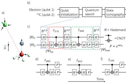
Figure 1: (a) Structure of the NV system with the electron spin coupled to one ¹⁴N and one ¹³C nuclear spin. (b) Schematic representation of the experimental procedure, including the initialization, the quantum search and the state tomography for determining the outcome, where (c) shows the gate sequence for searching the target state $|11\rangle$. $|\Psi\rangle_{in}$ denotes the equal superposition of all basis states. The output state $|\Psi\rangle_{out}$ is the target state $|11\rangle$. The circuits for the other target states $|00\rangle$, $|01\rangle$, $|10\rangle$ are obtained by replacing the phase flip operation $I_{|11\rangle}$ by $I_{|00\rangle}$, $I_{|01\rangle}$, $I_{|10\rangle}$, which can be implemented by the circuits shown in (d-f).

Experimental protocol.- For the experimental implementation we used a diamond with 99.995% ¹²C, and the concentration of substitutional nitrogen of $<10$ ppb to minimize decoherence Jahnke et al. (2012); Teraji et al. (2013); Zhang et al. (2013). The experimental setup is presented in the SM. The experiment was performed at room temperature in a static magnetic field $B$ of 14.8 mT along the symmetry axis of the NV center. The structure of the NV center with the coupled ¹⁴N and ¹³C nuclear spins is illustrated in Figure 1 (a). Here we use a symmetry-adapted coordinate system, where the $z$-axis is oriented along the NV axis, while the ¹³C nucleus is located in the $xz$-plane Rao and Suter (2016). In this context, we focus on the subsystem where the ¹⁴N is in the state $m_{N}$=1. The relevant Hamiltonian for the electron and ¹³C spins is then

$$\frac{\mathcal{H}_{e,C}}{2\pi}=DS_{z}^{2}-(\gamma_{e}B-A_{N})S_{z}-\gamma_{C}BI_{z}+A_{zz}S_{z}I_{z}+A_{zx}S_{z}I_{x}.$$ (1)

Here $S_{z}$ denotes the spin-1 operator for the electron and $I_{x/z}$ the ¹³C spin-1/2 operators. The zero-field splitting is $D=2.87$ GHz. $\gamma_{e/C}$ denote the gyromagnetic ratios for the electron and ¹³C spins, respectively. $A_{N}=-2.16$ MHz is the secular part of the hyperfine coupling between the electron and the ¹⁴N nuclear spin Shin et al. (2014); He et al. (1993); Yavkin et al. (2016), while $A_{zz}$ and $A_{zx}$ are the relevant components of the ¹³C hyperfine tensor, which are $A_{zz}=-0.152$ MHz and $A_{zx}=0.110$ MHz in the present system.

We select a 2 qubit system for implementing the quantum search by focusing on the subspace with the electron spin in $\{|0\rangle,|-1\rangle\}$ as qubit 1 and the ¹³C spin as the second qubit. Our computational basis $\{|0\rangle,|1\rangle\}_{1}\otimes\{|0\rangle,|1\rangle\}_{2}$ corresponds to the physical states $\{|0\rangle,|-1\rangle\}_{e}\otimes\{|\uparrow\rangle,|\downarrow\rangle\}_{C}$, where the states $|0\rangle$ and $|-1\rangle$ denote the eigenstates of $S_{z}$, $|\uparrow\rangle$ and $|\downarrow\rangle$ the eigenstates of $I_{z}$ with eigenvalues of $1/2$ and $-1/2$, respectively. Figure 1 (b) outlines the protocol for implementing the quantum search.

In the step of qubit initialization, we use a 4 $\mu s$, 0.5 mW pulse of 532 nm laser light to initialize the electron spin into the $m_{S}=0$ state. Additional details of the setup are presented in the Supplemental Material (SM) not , which includes Refs. Childress et al. (2006); Zhang et al. (2018a); Vandersypen and Chuang (2005); Zhang et al. (2018b). Based on the initialized electron spin, we further polarize the ¹³C spin by a combination of MW and laser pulses, and set the qubits into the pure state $|00\rangle$ Zhang et al. (2019); Hegde et al. (2020). Additional details are given in the SM.

The protocol for the actual quantum search is shown in Figure 1 (c) for the target state $|s_{t}\rangle=|11\rangle$. The circuits for the other target states $|00\rangle$, $|01\rangle$, and $|10\rangle$ are obtained by replacing the phase flip operation $I_{|11\rangle}$ by $I_{|00\rangle}$, $I_{|01\rangle}$, and $I_{|10\rangle}$, as shown in Figure 1 (d-f), respectively.

To implement the actual search shown as Figure 1 (c), we considered sequences of MW pulses with constant MW and Rabi frequencies but variable durations and phases. The MW frequencies were resonant with the ESR transitions between the electron states $m_{S}=0\leftrightarrow m_{S}=-1$. The pulse durations, phases and delays were used as variables in an optimization procedure based on optimal control (OC) theory Mitchell (1998); Zhang et al. (2019); Hegde et al. (2020) that maximizes the overlap between the operation generated by the sequence and the operation required by the quantum circuit of Figure 1 (c), which can reach unity in the ideal case D’Alessandro (2008); Hodges et al. (2008); Khaneja (2007).

The OC process has to balance several considerations. While it is helpful to use many pulses and therefore many degrees of freedom to optimize the theoretical fidelity of the gate operaation, additional pulses also increase the total duration of the sequence and therefore the effect of decoherence (mainly from the electron spin in the present work), and the experimental imperfections also tend to increase with the number of pulses. We found that sequences of 4 pulses and 5 delays to be a good compromise for all four target states, see details in SM.

To determine the state of the system after the search operation, we use the techniques developed in quantum state tomography Nielsen and Chuang (2000); Leskowitz and Mueller (2004), to reconstruct the populations or full quantum states. This requires a set of measurements applied to the output state $|\Psi\rangle_{out}$.

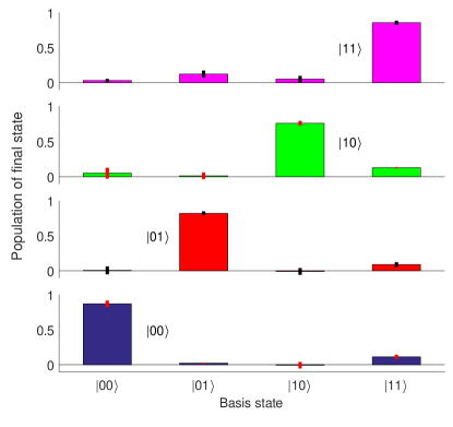
Figure 2: Experimentally measured populations of the four basis states after the quantum search with the targets $|00\rangle$, $|01\rangle$, $|10\rangle$, and $|11\rangle$, as indicated in the panels. The error bars indicate 1 standard deviation, which was determined by repeating each experiment.

Experimental results.- Figure 2 illustrates the experimental results for the different target states. Here we only show the populations obtained from partial tomography. The measured populations of the target states, or the probabilities of finding the target states, are $0.87\pm 0.05$, $0.82\pm 0.03$, $0.76\pm 0.03$ and $0.85\pm 0.03$ for the target states $|00\rangle$, $|01\rangle$, $|10\rangle$ and $|11\rangle$, with the sums of the populations $1.00\pm 0.03$, $0.90\pm 0.03$, $0.95\pm 0.06$ and $1.06\pm 0.02$, respectively. In each case the probability of finding the target state is much higher than the classical result of $0.25$. In the ideal case, the population of the target state should be 1 and the others 0. The deviation of the sum of the populations for each case from the unity can be mainly attributed to imperfections in the tomography, which cause population leakage to the electron state $m_{S}=1$. Secondly, the incomplete selectivity of the MW pulses leads to loss of population from the computational subspace. We estimate that this contribution is less than 0.027 in our experiments. The effects from the coupled ¹⁴N spin can be decreased, e.g., by polarizing ¹⁴N Xu et al. (2019); Chakraborty et al. (2017); Rama Koteswara Rao et al. (2020); Pagliero et al. (2014); Zu et al. (2014); Wang et al. (2015); Yun et al. (2019), where the polarization can be $>98\%$ Xu et al. (2019); Yun et al. (2019). The details are presented in the SM.

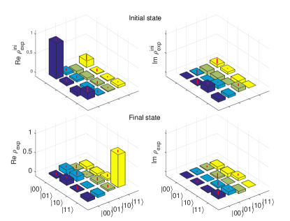
Figure 3: Measured density matrices for the prepared initial state $|00\rangle$ (top) and for the state after the completion of the quantum search with target state $|11\rangle$ (bottom). The real and imaginary parts are shown in the left and right columns.

Figure 3 shows the reconstruction of the full density matrices for the initial state and the search result for the target state $|11\rangle$. By calculating the fidelities as $F=Tr\{\rho_{th}\rho_{exp}\}$, we obtained $F_{ini}=0.92\pm 0.01$, and $F_{|11\rangle}=0.85\pm 0.03$, for the initial state and the final state after the quantum search. The loss of the fidelity in the quantum search can be attributed to the imperfection of the theoretical pulse sequence, the experimentally implemented sequence and the experimentally implemented initial state including the state tomography, in the order of importance. The details of the error estimation are presented in the SM.

Discussion.- The OC efficiency can be improved by maximizing the angle between the different quantization axes of the nuclear spin for the different states of the electron spin Khaneja (2007). The experimental fidelity might be improved further, e.g., by increasing the robustness with respect to fluctuations of the Rabi frequency (see examples in the SM, Section VIIA), and increasing the Rabi frequency Zhang et al. (2019), e.g., in the case that the ¹⁴N is polarized. Moreover, the choice of a more efficient optimal algorithm should be helpful Yang (2020); Weise (2009). To estimate the scalability of the OC scheme in larger systems, we use numerical simulation of systems with one electron spin and $n=1$, …, 4 ¹³C spins. As examples, we use 3-4 MW pulses with 4-5 delays to implement the CNOT-like gates, where the electron spin (in the subspace $m_{S}=0$ and $m_{S}=-1$) acts as the control qubit, while one ¹³C spin is the target qubit. The target operation is chosen as $R_{x}^{j}(\pi)=e^{-i\pi I_{x}^{j}}$, where $j$ indicates the target ¹³C spin. The details are presented in the SM.

We investigate the dependence of the gate fidelity and duration on the number of the qubits in the system. The results are shown in Figure 4, and the parameters for the pulse sequences are presented in the SM. The results show that the ¹³C spin quanzitation axis orientation in the subspace $m_{S}=-1$, denoted as $\theta_{-}$ in Figure 4 (a), is a crucial factor in the optimization. The quality of the gate, here evaluated by the gate fidelity and duration, is degraded only marginally by the passive ¹³C spins coupled to the electron. For example, for $j=1$, with $\theta_{-}=87{}^{\circ}$, the gate fidelity is higher than $0.995$, and the gate duration remaims in the range of 16 - 18 $\mu$s for up to 5 qubits. In other cases, with $\theta_{-}$ in the range of $97-118^{\circ}$, we obtain fidelities in the range of 0.930 - 0.995, with gate durations of 11 - 23 $\mu$s. The fidelity can be improved further by increasing the number of MW pulses.

Since the CNOT gate can be combined with single-qubit gates to yield a universal set of gatesNielsen and Chuang (2000); Cappellaro et al. (2009), the method presented in this paper represents a universal solution for implementing quantum computing.

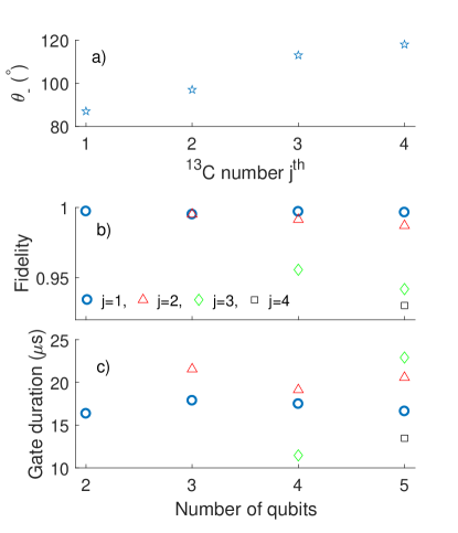
Figure 4: (a) The quantization axis orientation of $j$th ¹³C spin of the subspace $m_{S}=-1$ between $z$- axis, the orientation of the subspace $m_{S}=0$. (b-c) Results by simulation of controlled- $R_{x}^{j}(\pi)$ (CNOT-like gates) in 2-5 qubit systems, respectively, where the electron spin is the control qubit, and $R_{x}^{j}(\pi)=e^{-i\pi I_{x}^{j}}$ with $j$ indicating the affected ¹³C spin. Figures (b-c) show the gate fidelity and duration, respectively.

Conclusion.- We have experimentally implemented Grover’s quantum search algorithm in a hybrid quantum register in a single NV center in diamond by indirect control: control pulses were applied only to the electron spin, which has a much fast response time than the nuclear spins. In a 2 qubit system, we implemented 4 cases of the quantum search, in each of which one target state was searched. The whole procedure for demonstrating the quantum algorithm was implemented, including the preparation of the pure state, implementation of the quantum search and reconstruction of the output state. For each target state, the complete search algorithm was implemented with only 4 MW pulses. This corresponds to a significant reduction of the control cost compared with previous works. Further improvements should be possible by designing the pulse sequence robust against dephasing effects, or by combining the operations with dynamical decoupling techniques Zhang et al. (2014); Zhang and Suter (2015); Souza et al. (2012); Suter and Álvarez (2016).

Acknowledgments.- This project has received funding from the European Union’s Horizon 2020 research and innovation programme under grant agreement No 828946. The publication reflects the opinion of the authors; the agency and the commission may not be held responsible for the information contained in it. We thank Daniel Burgarth for helpful discussions.

Supplemental Material

.1 Setup for optical initialization and detection

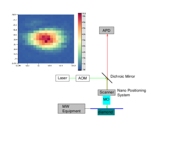
Figure 5: Schematic of the confocal microscope for initializing and detecting single NV centers. The inset shows an image of the single NV center we used in the experiment.

Single NV centers in diamond can be optically addressed, initialized and detected with a confocal microscope (Suter and Jelezko, 2017). In Fig. 5 we show a schematic of our home-built setup. Here we used a diode-pumped solid state continuous wave laser with a wavelength of 532 nm (marked in green in the schematic) for the optical excitation. For pulsed experiments, an acousto-optical modulator (AOM) with 58 dB extinction ratio and 50 ns rise-time generated the pulses from the continuous wave laser beam. The microscope objective (MO) lens was fixed to the nano positioning system that scans the sample in three dimensions. The fluorescence light with around 637 nm wavelength (marked in red in the schematic) is also collected by this MO lens, and passes the dichroic mirror to the avalanche photodiode (APD) detector. The excitation light is filtered out by the dichroic mirror.

.2 System and Hamiltonian

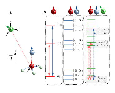
Figure 6: Characteristics of the system. (a) Structure of the NV system with the electron spin coupled to one ¹⁴N and one ¹³C nuclear spin. (b) Energy levels of the system consisting of the electron, ¹⁴N and ¹³C nuclear spins. The vertical double arrows indicate the ESR transitions that we use in this work.

As illustrated in Figure 6, the spin system used in the present work consists of the electron, ¹⁴N and ¹³C nuclear spins. The static magnetic field $\vec{B}$ is aligned along the N-V symmetry axis $z$. The relevant Hamiltonian can be written as

$$\mathcal{H}/(2\pi) = DS_{z}^{2}-\gamma_{e}BS_{z}+P(I_{z}^{N})^{2}-\gamma_{N}BI_{z}^{N}-\gamma_{C}BI_{z}$$ (2)

$$+ A_{N}S_{z}I_{z}^{N}+A_{zz}S_{z}I_{z}+A_{zx}S_{z}I_{x}.$$

Here $S_{z}$ and $I_{z}^{N}$ denote the spin-1 operators for the electron and ¹⁴N spins and $I_{x/z}$ the ¹³C spin-1/2 operators. In frequency units, the zero-field splitting is $D=2.87$ GHz, and the ¹⁴N nuclear quadrupole coupling is $P=-4.95$ MHz. $\gamma_{e/N/C}$ denote the gyromagnetic ratios for the electron, ¹⁴N and ¹³C spins, respectively. $A_{N}=-2.16$ MHz is the secular part of the hyperfine coupling with the ¹⁴N nuclear spin (Shin et al., 2014; He et al., 1993; Yavkin et al., 2016), while $A_{zz}$ and $A_{zx}$ are the relevant components of the ¹³C hyperfine tensor, which are $A_{zz}=-0.152$ MHz and $A_{zx}=0.110$ MHz in the present system.

In Figure 7 we show the ESR spectra, obtained from a Free Induction Decay (FID) experiment (Childress et al., 2006; Zhang et al., 2018a). The pulse sequence is shown as the inset in Figure 7 (a). The wavelength of the laser pulses is 532 nm, the laser power $\approx$0.5 mW. The first laser pulse (duration $4$ $\mu$s) initializes the electron spin into state $m_{S}=0$. The second laser pulse (duration $0.4$ $\mu$s) is used to detect the population of the state $m_{S}=0$ (Suter and Jelezko, 2017).

The MW pulses are on resonance with the transition $m_{S}=0$ $\leftrightarrow$ $m_{S}=-1$ or $m_{S}=0$ $\leftrightarrow$ $m_{S}=1$, for the spectrum in Figure 7 (a) or (b), respectively. In each case, the pulses have high enough Rabi frequency to cover all the transitions: in (a), the Rabi frequency is 8.5 MHz, and in (b) 3.7 MHz. The two MW pulses are both rectangular pulses with flip angle $\pi/2$. The first pulse generates coherence between states $m_{S}=0$ and $m_{S}=-1$ (a) or $m_{S}=0$ and $m_{S}=1$ (b). After the pulse, the system evolves under the Hamiltonian (2). The second MW pulse converts the evolved coherence to population, so that it can be detected by the detection laser pulse. The phase of the second MW pulse is set as $\phi=2\pi\nu_{d}t$ to generate an effective offset $\nu_{d}$ in the spectrum, such that all resonance lines appear at positive frequencies.

If we focus on a subspace where the state of the ¹⁴N is fixed ($m_{N}=1$ in the main text), $\mathcal{H}_{e,C}$ shown in Eq. (1) in the main text can be diagonalized by the unitary transformation

$$U_{tr}=|1\rangle\langle 1|\otimes R_{y}(\theta_{+})+|0\rangle\langle 0|\otimes E+|-1\rangle\langle-1|\otimes R_{y}(\theta_{-}),$$ (3)

where $E$ denotes the $2\times 2$ identity operator and $R_{y}(\theta_{\pm})=e^{-i\theta_{\pm}I_{y}}$. The nuclear-spin eigenstates are

$$|\varphi_{\pm}\rangle = |\uparrow\rangle\cos(\theta_{\pm}/2)+|\downarrow\rangle\sin(\theta_{\pm}/2)$$

$$|\psi_{\pm}\rangle = -|\uparrow\rangle\sin(\theta_{\pm}/2)+|\downarrow\rangle\cos(\theta_{\pm}/2)$$ (4)

where $\theta_{\pm}=\arctan[A_{zx}/(A_{zz}\mp\nu_{C})]$ denotes the angle between the nuclear spin quantization axis and the $z$-axis of our coordinate system for the subsystems where the electron spin is in $m_{S}=\pm 1$. From the experimental spectra, we found $\theta_{-}=87^{\circ}$ and $\theta_{+}=-10^{\circ}$. These results show that the quantization axis of ¹³C for $m_{S}=-1$ ($m_{S}=1$) is approximately perpendicular to (parallel) to the axis for $m_{S}=0$, respectively, and explain why the hyperfine splitting from ¹³C results in four (two) satellites, as shown in Figure 7 (a-b) (Zhang et al., 2019).

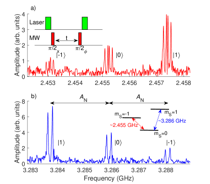
Figure 7: ESR spectra obtained by ODMR with the pulse sequence [inset in (a)]. The spectra are obtained in a field of $B=14.8$ mT for the transitions between (a) $m_{S}=0\leftrightarrow-1$ and (b) $m_{S}=0\leftrightarrow+1$ , as illustrated in the inset in (b)]. The labels $|0\rangle$, $|1\rangle$, and $|-1\rangle$ mark the state of the ¹⁴N spin. The horizontal double arrows indicate the hyperfine coupling with ¹⁴N.

.3 Pulse Sequences

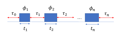
Figure 8: Pulse sequence with $n$ pulses and $n+1$ delays for implementing arbitrary unitary ${\cal U}$. The parameters $t_{i}$ are MW pulse durations, $\phi_{i}$ are the phases and $\tau_{j}$ the delays. The amplitude of the pulses is fixed to a Rabi frequency $\omega_{1}/(2\pi)$ = 0.5 MHz, or a value in $[0.48,0.52]$ for the sequence that is robust against variations in $\omega_{1}$.

In a subspace spanned by the states

$$\{|0\rangle,|-1\rangle\}_{e}\otimes\{|1\rangle\}_{N}\otimes\{|\uparrow\rangle,|\downarrow\rangle\}_{C},$$ (5)

the Hamiltonian of the electron-¹³C system can be represented as

$$\frac{1}{2\pi}\mathcal{H}_{s}=(-\nu_{C}-\frac{A_{zz}}{2})I_{z}+A_{zz}s_{z}I_{z}+A_{zx}s_{z}I_{x}-\frac{A_{zx}}{2}I_{x}$$ (6)

in the rotating frame (Vandersypen and Chuang, 2005) with transform $U_{r}=e^{-i2\pi\nu_{r}ts_{z}}$ where $\nu_{r}=D+\nu_{e}-A_{N}$. Here $s_{z}$ denotes the pseudo-spin 1/2 operator for the electron spin in the subspace and $\nu_{C}=\gamma_{C}B$.

The pulse sequence to implement an arbitrary target unitary ${\cal{U}}$ is shown as Figure 8, where $n$ MW pulses with fixed Rabi frequency $\omega_{1}$ and $n+1$ delays are used. The propagators for the individual MW pulses can be written as $U_{k}^{MW}=e^{-i\mathcal{H}_{k}^{MW}t_{k}}$ where $\mathcal{H}_{k}^{MW}=\mathcal{H}_{s}+\omega_{1}[s_{x}\cos(\phi_{k})+s_{y}\sin(\phi_{k})]$, with $k=1,\cdots,n$, and for the free evolutions as $U_{k}^{d}=e^{-i\mathcal{H}_{s}\tau_{k}}$, with $k=0,\cdots,n$. The total unitary ${\cal U}$ is a time ordered product of the $U_{k}^{MW}$ and $U_{k}^{d}$, and is a function of the pulse parameters $(t_{1},\cdots,t_{n},\phi_{1},\cdots,\phi_{n},\tau_{0},\cdots,\tau_{n})$. The goal is to design a unitary ${\cal U}$ that maximizes the fidelity

$$F_{g}=|\mathrm{Tr(U_{T}^{\dagger}{\cal U}})|/4$$ (7)

where $U_{T}$ denotes the target unitary operation. We used a genetic algorithm for the numerical search to obtain an optimal set of parameters.

In the experiment of the Grover’s quantum search, we use one pulse sequence with $4$ MW pulses and 5 delays to implement the circuit shown in Figure 1 (c) in the main text for each target state. The effect of the individual MW pulses is sensitive to variations in $\omega_{1}$. In Figure 9, we illustrate the fluctuation of $\omega_{1}/(2\pi)$ over 7 hours. The fluctuation of MW power could be mainly attributed to the amplifiers in the circuit, where we used three amplifiers in series from mini circuits [models ZHL-16W-43-S+ (power amplifier), ZFL-500LN+ (pre-amplifier) and ZX60-4016E-S+ (pre-amplifier)].

As shown in Figure 9 the MW field strength (Rabi frequency) varies by about 0.03 MHz over the time scale of the experiment (3 hours). To obtain good fidelity in experiments where the actual MW amplitude deviates from the ideal one, we optimized the pulse sequences for a range of amplitudes, taking the average fidelity as the performance measure, so that the resulting sequences are robust against the amplitude fluctuation. We used the range $\omega_{1}/2\pi=[0.48,0.52]$ MHz, which covers the observed range of amplitudes, as shown in Figure 9. The theoretical fidelities for the targets $|00\rangle$, $|01\rangle$, $|10\rangle$ and $|11\rangle$ are $98.2\%$, $97.9\%$, $98.0\%$ and $97.1\%$, respectively. The parameters of the pulse sequences are listed in Tables 1(a) - 1(d).

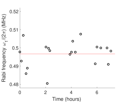
Figure 9: Variation of the Rabi frequency $\omega_{1}/(2\pi)$ with time. The red line indicates the average.

Delay ($\mu$s)	Pulse duration ($\mu$s)	Phase (∘)
$\tau_{0}=0.987$
$\tau_{1}=1.968$	$t_{1}=0.976$	$\phi_{1}=261$
$\tau_{2}=2.418$	$t_{2}=0.510$	$\phi_{2}=213$
$\tau_{3}=2.465$	$t_{3}=0.394$	$\phi_{3}=141$
$\tau_{4}=1.136$	$t_{4}=1.104$	$\phi_{4}=90$

(a) Target $|00\rangle$.

Delay ($\mu$s)	Pulse duration ($\mu$s)	Phase (∘)
$\tau_{0}=0.559$
$\tau_{1}=0.399$	$t_{1}=0.555$	$\phi_{1}=302$
$\tau_{2}=2.905$	$t_{2}=1.290$	$\phi_{2}=195$
$\tau_{3}=2.476$	$t_{3}=0.472$	$\phi_{3}=196$
$\tau_{4}=1.139$	$t_{4}=1.423$	$\phi_{4}=90$

(b) Target $|01\rangle$.

Delay ($\mu$s)	Pulse duration ($\mu$s)	Phase (∘)
$\tau_{0}=0.995$
$\tau_{1}=2.518$	$t_{1}=1.484$	$\phi_{1}=102$
$\tau_{2}=2.353$	$t_{2}=0.542$	$\phi_{2}=340$
$\tau_{3}=0.361$	$t_{3}=0.210$	$\phi_{3}=47$
$\tau_{4}=1.191$	$t_{4}=1.262$	$\phi_{4}=90$

(c) Target $|10\rangle$.

Delay ($\mu$s)	Pulse duration ($\mu$s)	Phase (∘)
$\tau_{0}=1.892$
$\tau_{1}=2.345$	$t_{1}=0.995$	$\phi_{1}=198$
$\tau_{2}=2.583$	$t_{2}=0.541$	$\phi_{2}=0$
$\tau_{3}=2.576$	$t_{3}=0.452$	$\phi_{3}=90$
$\tau_{4}=0.665$	$t_{4}=0.939$	$\phi_{4}=90$

(d) Target $|11\rangle$.

Table 1: Parameters for the pulse sequence robust against the fluctuation of the MW amplitude to implement Grover’s search with various target states.

.4 Error analysis

Based on the measured density matrices shown in Figure 3 in the main text, we evaluate the performance of the quantum search in the following way.

1. As listed in the main text, the experimental fidelity of the initial state $\rho_{exp}^{ini}$ is $F_{ini}=0.92$. The loss of fidelity can be mainly attributed to the imperfection of the tomography. Examples include the non-negligible off-diagonal elements in the density matrix, which reflect imperfect tomography. By applying the ideal circuit of Figure 1(c) in the main text to $\rho_{exp}^{ini}$, we obtain $\rho_{1}$, and then calculate the state fidelity $F_{1}=Tr\{\rho_{th}\rho_{1}\}=0.925$, where $\rho_{th}=|11\rangle\langle 11|,$ which is close to $F_{ini}$. Since we used the same tomography procedure for the initial and the final state, we conclude that the main contribution to the observed infidelity originates from the tomographic analysis.

2. By applying the theoretical MW pulse sequence to the ideal initial state $\rho^{ini}=|00\rangle\langle 00|$, we obtain $\rho_{2}=U_{MW}\rho^{ini}U_{MW}^{\dagger}$, and the fidelity $F_{2}=Tr\{\rho_{th}\rho_{2}\}=0.967.$

3. Combining the measured fidelity $F_{|11\rangle}=0.85$ for Grover’s search obtained from the results shown in Figure 3 in the main text, we estimate the fidelity of the implemented quantum search as $F_{3}=F_{|11\rangle}/(F_{1}F_{2})=0.95$. In our system, we can treat the decoherence time of the electron spin between $T_{2}^{*}\approx 35\mu$s measured from the ESR FID signal and $T_{2}\approx 1$ ms from the dynamical decoupling sequence (Zhang et al., 2018b). The duration of the pulse sequence is 12.989 $\mu$s, which is not negligible compared to $T_{2}^{*}$. Therefore the decoherence appears to be the main contibution to the error in the search. Increasing the coherence time of the electron spin, e.g., by decreasing the concentration of substitutional nitrogen spins in the diamod sample, should further improve the experiment.

   .5 Effects of ¹⁴N in Grover’s search

   The MW pulse sequences for implementing Grover’s search targeted the subspace of ¹⁴N state $m_{N}=1$, where $m_{N}$ denotes magnetic quantum number for ¹⁴N spin. We here simulated the pulse sequences applied to the whole space of ¹⁴N as $m_{N}=\{0,-1,1\}$ to investigate the quality of selectivity for the subspace of $m_{N}=1$. To simplify the procedure, we here only consider the electron and the ¹⁴N spins (Zhang et al., 2018a). For our system, the initial state can be represented as (Zhang et al., 2019)

   $$\rho_{0}^{e,N}=|0\rangle\langle 0|_{e}\otimes\left(\sum c_{m_{N}}|m_{N}\rangle\langle m_{N}|\right)$$ (8)

   where $c_{m_{N}}\approx 4/7$, $2/7$, $1/7$, for $m_{N}=1$, $0$, $-1$ (Zhang et al., 2019). In the ideal case, the MW pulses that are set to select the subspace of $m_{N}=1$ do not change the populations of the states $|0,0\rangle$ and $|0,-1\rangle$ in the initial state (8).

   After applying the pulse sequence to the initial state $\rho_{0}^{e,N}$, we measured the populations of states $|0,0\rangle$ and $|0,-1\rangle$, and found that they decreased from the initial values.

   In the procedure of state tomography in experiment, we extracted the population of the state $|0,1\rangle$ by subtracting initial populations of states $|0,0\rangle$ and $|0,-1\rangle$ [given by $c_{0}$ and $c_{-1}$ in Eq. (8)] from the total population of the bright electron state $m_{S}=0$. Therefore the changes of the populations of states $|0,0\rangle$ and $|0,-1\rangle$ in Grover’s search lead to a loss of measured population of the computational subspace of $m_{N}=1$. In Table 2, we list the loss of population in Grover’s search for each target state.

   Target state in Grover’s search	Loss of the population
   $|00\rangle$	0.025
   $|01\rangle$	0.0068
   $|10\rangle$	0.020
   $|11\rangle$	0.027

   Table 2: The loss of the population of the computational subspace in Grover’s search due to effects of the ¹⁴N coupled to the electron spin.

   We use numerical simulation to investigate the dependence of the loss of the population $L_{p}$ on the polarization of the ¹⁴N spin $p_{N}$ using the case of the target state $|11\rangle$ as an example. The input state is

   $$\rho_{0,sim}^{e,N}=|0\rangle\langle 0|_{e} \otimes (p_{N}|1\rangle\langle 1|+\frac{1-p_{N}}{2}|0\rangle\langle 0|$$ (9)

   $$+ \frac{1-p_{N}}{2}|-1\rangle\langle-1|)$$

   The pulse sequence in simulation is shown in Figure 8, with the parameters listed in Table 1(d). We calculated the sum of the populations in the states $|m_{S}=-1,m_{N}=0\rangle$ and $|m_{S}=-1,m_{N}=-1\rangle$ as the loss of the population $L_{p}$ from the computational space. Figure 10 shows the result.

   

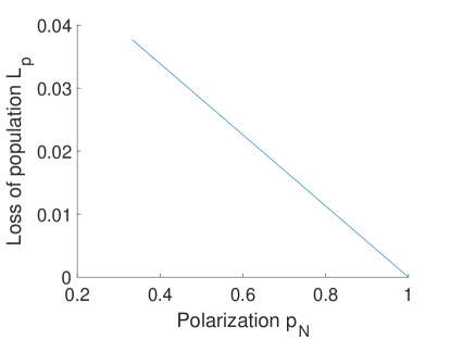
   Figure 10: Dependence of the loss of population $L_{p}$ on the initial polarization of the ¹⁴N spin $p_{N}$. The range of $p_{N}$ was chosen from $1/3$ to $1$, corresponding to the ¹⁴N in the maximal mixed ( or identity) state and pure state with $m_{N}=1$.

   .6 Pulse sequence for pure state preparation

   

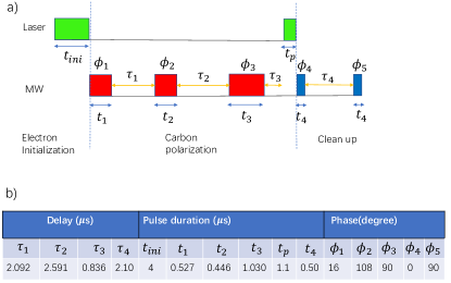
   Figure 11: Pulse sequence (a) with the parameters listed in table (b) for preparing the pure state $|00\rangle$. The amplitude of the pulses is fixed to a Rabi frequency $\omega_{1}/(2\pi)$ = 0.5 MHz. The MW pulses indicated in red rectangles are on resonance with the transition frequency between $m_{S}=0$ and $-1$, those in blue with $m_{S}=0$ $\leftrightarrow$ $1$. The clean up step is a CNOT-like gate (Zhang et al., 2018a) that moves the leftover (undesired) population of state $|01\rangle$ out of the computational space.

   Figure 11 (a) shows the pulse sequence to prepare the pure state $|00\rangle$, and (b) the parameters (Zhang et al., 2019). In the initialization step, the electron is set to $m_{S}=0$, while the ¹³C spin is in the maximally mixed state. The ¹³C spin can be polarized by the MW and laser pulses indicated in the step of carbon polarization. The state of the two spins after the second laser pulse can be represented as

   $$\rho_{p}=|0\rangle\langle 0|\otimes[p|0\rangle\langle 0|+(1-p)|1\rangle\langle 1|+c(|0\rangle\langle 1|+|1\rangle\langle 0|)]$$ (10)

   with $p$ measured as 0.83, and c as 0.08. The state $\rho_{p}$ can be further purified by moving the leftover population of state $|01\rangle$ and the coherence out of the space for quantum computing (Hegde et al., 2020). As a result, we obtain a pure state $\rho^{ini}=|00\rangle\langle 00|$ as the initial state for the quantum search, after re-normalizing the total population in the two qubit computational space to unity.

   .7 Additional data for optimal control

   .7.1 Parameters of the pulse sequence with fixed Rabi of $0.5$ MHz

   If we assume that the amplitude of the MW pulses can be exactly controlled, e.g., the Rabi frequency $\omega_{1}$ is fixed to $0.5$ MHz, we can remove the condition of robustness against fluctuations of $\omega_{1}$ from the optimization of the parameters, and therefore we can increase the theoretical fidelity of the pulse sequence. We list the resulting parameters in Tables 3(a) -3(d). The average fidelity for the four target states is $0.988$, slightly higher than in the robust case, which is $0.980$, obtained from the parameters listed in Tables 1(a) -1(d). The average duration of the pulse sequences for the four target states is $12.2$ $\mu$s, similar to the robust case where it was $11.8$ $\mu$s.

   If we use 6 MW pulses instead of 4, we can improve the fidelity in the case of target state $|01\rangle$ to $0.995$, with a sequence duration of $19.23$ $\mu$s. The parameters are llisted in Table 4.

   Delay ($\mu$s)	Pulse duration ($\mu$s)	Phase (∘)
   $\tau_{0}=0.944$
   $\tau_{1}=1.922$	$t_{1}=1.139$	$\phi_{1}=266$
   $\tau_{2}=2.554$	$t_{2}=0.481$	$\phi_{2}=201$
   $\tau_{3}=1.802$	$t_{3}=0.402$	$\phi_{3}=142$
   $\tau_{4}=0.777$	$t_{4}=1.126$	$\phi_{4}=90$

   (a) Target state $|00\rangle$, with theoretical fidelity 0.991.

   Delay ($\mu$s)	Pulse duration ($\mu$s)	Phase (∘)
   $\tau_{0}=1.099$
   $\tau_{1}=0.608$	$t_{1}=0.479$	$\phi_{1}=285$
   $\tau_{2}=2.442$	$t_{2}=0.881$	$\phi_{2}=2$
   $\tau_{3}=2.993$	$t_{3}=0.608$	$\phi_{3}=197$
   $\tau_{4}=1.768$	$t_{4}=1.323$	$\phi_{4}=90$

   (b) Target state $|01\rangle$, with theoretical fidelity 0.984.

   Delay ($\mu$s)	Pulse duration ($\mu$s)	Phase (∘)
   $\tau_{0}=0.634$
   $\tau_{1}=1.763$	$t_{1}=1.698$	$\phi_{1}=112$
   $\tau_{2}=1.603$	$t_{2}=0.448$	$\phi_{2}=313$
   $\tau_{3}=1.945$	$t_{3}=0.426$	$\phi_{3}=23$
   $\tau_{4}=1.261$	$t_{4}=1.224$	$\phi_{4}=90$

   (c) Target state $|10\rangle$, with theoretical fidelity 0.990.

   Delay ($\mu$s)	Pulse duration ($\mu$s)	Phase (∘)
   $\tau_{0}=1.751$
   $\tau_{1}=2.439$	$t_{1}=1.069$	$\phi_{1}=10$
   $\tau_{2}=1.661$	$t_{2}=1.584$	$\phi_{2}=125$
   $\tau_{3}=3.255$	$t_{3}=0.514$	$\phi_{3}=51$
   $\tau_{4}=1.183$	$t_{4}=0.858$	$\phi_{4}=90$

   (d) Target state $|11\rangle$, with theoretical fidelity 0.990.

   Table 3: Parameters of the non-robust pulse sequences to implement Grover’s search with various target states.

   Delay ($\mu$s)	Pulse duration ($\mu$s)	Phase (∘)
   $\tau_{0}=0.887$
   $\tau_{1}=0.834$	$t_{1}=1.305$	$\phi_{1}=192$
   $\tau_{2}=2.994$	$t_{2}=1.570$	$\phi_{2}=46$
   $\tau_{3}=1.994$	$t_{3}=1.528$	$\phi_{3}=326$
   $\tau_{4}=1.734$	$t_{4}=0.770$	$\phi_{4}=54$
   $\tau_{5}=1.204$	$t_{5}=0.709$	$\phi_{5}=238$
   $\tau_{6}=2.598$	$t_{6}=1.103$	$\phi_{6}=90$

   Table 4: Parameters for the pulse sequence to implement Grover’s search with target state $|01\rangle$ with 6 pulses. The theoretical fidelity is 0.995.

   .7.2 Number of MW pulses

   We use the optimization of the pulse sequence for the Grover’s search with target state as $|01\rangle$ as an example to illustrate how to choose the number of the MW pulses in the optimal control. Figure 12 shows the obtained fidelities and gate durations when we used 3, 4 and 6 pulses, respectively. As expected, the fidelity increases with the number of pulses. However, it also leads to longer gate duration (except the case from 3-4 pulses, but the fidelity of 3 pulses is not high enough), and therefore enhance the effects of dephasing. Moreover, more pulses also result in more operation errors in experimental implementation. We chose 4 puslse as a compromise for the implementation of the Grover’s search.

   

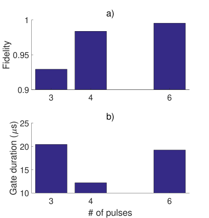
   Figure 12: Dependence of the fidelity (a) and gate duration (b) on the number of the MW pulses in the optimal control for the Grover’s search for the target state $|01\rangle$.

   .7.3 Comparison of optimization for CNOT-like gate and quantum search

   We compare the optimization of the pulse sequences for two unitaries. One unitary is chosen as a CNOT-like gate, where the electron spin acts as the control qubit, and ¹³C spin as the target. The operation for the target qubit is a rotation $R_{x}(\pi)=e^{-i\pi I_{x}}$ . The other unitary is Grover’s search for the target state $|11\rangle$ shown in Figure 1 (c). To clarify this circuit consisting of two CNOT-like gates (instead of CNOT gates) and 5 more single qubit gates, we represented this circuit as Figure 13 (a), where the dash-dotted rectangles indicate CNOT-like gates.

   In Figures 13 (b-c), we illustrate the decrease of the infidelity $1-F_{g}$ (or the increase of the gate fidelity $F_{g}$), with the generations (or iterations) in the optimization. It shows that the optimization for the CNOT-like gate is much faster than for Grover’s search which is more compex than the CNOT-like gate. The parameters are listed in Tables 6(a) and 3(d), respectively.

   Figure 13: (a) The simplified circuit for implementing Grover’s search with target state $|11\rangle$, identical to the circuit in Figure 1 (c) in the main text. In figure (a), the operations indicated in the solid rectangles denote single-qubit rotations $(\theta)_{\phi}=e^{-i\theta[I_{x}\cos(\phi)+I_{y}\sin(\phi)]}$ or $e^{-i\theta[s_{x}\cos(\phi)+s_{y}\sin(\phi)]}$, applied to ¹³C (bottom line) or electron (top line) spin, respectively. The dash-dotted rectangles indicate the CNOT-like gates. (b-c) The minimization of $1-F_{g}$ by the genetic algorithm with the generations during the optimization process for the CNOT-like gate and Grover’s quantum search with target state $|11\rangle$, as indicated in the panels, respectively. The gate fidelity $F_{g}$ is $>0.997$ for the CNOT-like gate, and $>0.990$ for the quantum search.

   .8 Simulation of multiple qubits system

   

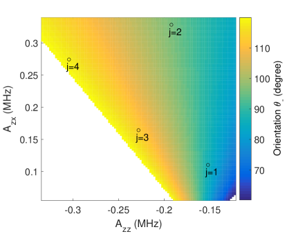
   Figure 14: The orientation of the quantization axis in the subspace of electron state $m_{S}=-1$ as a function of the coupling constants $A_{zz}$and $A_{zx}$.

   By generalizing the Hamiltonian (6) for the two spin system, we can write the Hamiltonian of one electron and $n$- ¹³C spins as

   $$\frac{1}{2\pi}\mathcal{H}_{m}=\sum_{j}^{n}[(-\nu_{C}-\frac{A_{zz}^{j}}{2})I_{z}^{j}+A_{zz}^{j}s_{z}I_{z}^{j}+A_{zx}^{j}s_{z}I_{x}^{j}-\frac{A_{zx}^{j}}{2}I_{x}^{j}].$$ (11)

   Here $I_{z/x}^{j}$ denotes the $z/x$ spin operator for $j$th ¹³C spin, and $A_{zz/zx}^{j}$ the couplings with the electron.

   Figure 14 shows the dependence of the ¹³C quantization axis orientation $\theta_{-}$ in the subspace of electron state $m_{S}=-1$ on the coupling strengths. Since for $m_{S}=0$ the quantization axis is aligned with the $z$-axis, $\theta_{-}$ is also the difference between the orientations. Here we only consider angles close to $90^{\circ}$, since these values offer high control efficiency (Khaneja, 2007). The couplings we used in the simulation are indicated by circles in Figure 14, and we list the values in Table 5.

   13C number $j$	$A_{zz}^{j}$ (MHz)	$A_{zx}^{j}$ (MHz)	Quantization axis $\theta_{-}$
   $1$	$-0.152$	$0.110$	$87^{\circ}$
   $2$	$-0.198$	$0.328$	$97^{\circ}$
   $3$	$-0.228$	$0.164$	$113^{\circ}$
   $4$	$-0.304$	$0.274$	$118^{\circ}$

   Table 5: Couplings of the $j^{\text{th }}$ ¹³C with the electron spin.

   We still use the method presented in Section .3 to optimize the pulse sequence. Here we use 3-4 MW pulses with 4-5 delays to implement the controlled-$R_{x}^{j}(\pi)$ with one ¹³C spin as the target qubit, where $R_{x}^{j}(\pi)=e^{-i\pi I_{x}^{j}}$ with $j$ indicating the affected ¹³C spin. The Rabi frequency is 0.5 MHz for 2-4 qubit system, but 1 MHz in the 5 qubit system. The parameters and the obtained fidelities are listed in Table 6.

   Delay ($\mu$s)	Pulse duration ($\mu$s)	Phase (∘)
   $\tau_{0}=3.452$
   $\tau_{1}=2.059$	$t_{1}=1.910$	$\phi_{1}=179$
   $\tau_{2}=2.124$	$t_{2}=3.888$	$\phi_{2}=136$
   $\tau_{3}=1.000$	$t_{3}=1.915$	$\phi_{3}=90$

   (a) Controlled-$R_{x}^{1}(\pi)$ in 2 qubits, with fidelity as 0.997.

   Delay ($\mu$s)	Pulse duration ($\mu$s)	Phase (∘)
   $\tau_{0}=3.294$
   $\tau_{1}=1.304$	$t_{1}=0.766$	$\phi_{1}=284$
   $\tau_{2}=2.707$	$t_{2}=0.222$	$\phi_{2}=235$
   $\tau_{3}=2.952$	$t_{3}=1.160$	$\phi_{3}=94$
   $\tau_{4}=2.463$	$t_{4}=3.006$	$\phi_{4}=90$

   (b) Controlled-$R_{x}^{1}(\pi)$ in 3 qubits, with fidelity as 0.995.

   Delay ($\mu$s)	Pulse duration ($\mu$s)	Phase (∘)
   $\tau_{0}=1.070$
   $\tau_{1}=1.679$	$t_{1}=3.612$	$\phi_{1}=87$
   $\tau_{2}=3.071$	$t_{2}=3.924$	$\phi_{2}=263$
   $\tau_{3}=3.711$	$t_{3}=0.370$	$\phi_{3}=224$
   $\tau_{4}=3.702$	$t_{4}=0.415$	$\phi_{4}=90$

   (c) Controlled-$R_{x}^{2}(\pi)$ in 3 qubits, with fidelity as 0.995.

   Delay ($\mu$s)	Pulse duration ($\mu$s)	Phase (∘)
   $\tau_{0}=1.384$
   $\tau_{1}=1.615$	$t_{1}=2.163$	$\phi_{1}=113$
   $\tau_{2}=3.286$	$t_{2}=0.133$	$\phi_{2}=15$
   $\tau_{3}=5.199$	$t_{3}=1.126$	$\phi_{3}=141$
   $\tau_{4}=1.375$	$t_{4}=1.202$	$\phi_{4}=90$

   (d) Controlled-$R_{x}^{1}(\pi)$ in 4 qubits, with fidelity as 0.997.

   Delay ($\mu$s)	Pulse duration ($\mu$s)	Phase (∘)
   $\tau_{0}=0.981$
   $\tau_{1}=2.490$	$t_{1}=0.963$	$\phi_{1}=253$
   $\tau_{2}=5.768$	$t_{2}=1.543$	$\phi_{2}=202$
   $\tau_{3}=1.411$	$t_{3}=0.370$	$\phi_{3}=72$
   $\tau_{4}=4.837$	$t_{4}=0.765$	$\phi_{4}=90$

   (e) Controlled-$R_{x}^{2}(\pi)$ in 4 qubits, with fidelity as 0.991.

   Delay ($\mu$s)	Pulse duration ($\mu$s)	Phase (∘)
   $\tau_{0}=1.277$
   $\tau_{1}=1.742$	$t_{1}=0.758$	$\phi_{1}=212$
   $\tau_{2}=2.903$	$t_{2}=0.751$	$\phi_{2}=60$
   $\tau_{3}=0.744$	$t_{3}=1.076$	$\phi_{3}=87$
   $\tau_{4}=0.719$	$t_{4}=1.490$	$\phi_{4}=90$

   (f) Controlled-$R_{x}^{3}(\pi)$ in 4 qubits, with fidelity as 0.956.

   Delay ($\mu$s)	Pulse duration ($\mu$s)	Phase (∘)
   $\tau_{0}=3.428$
   $\tau_{1}=4.375$	$t_{1}=0.354$	$\phi_{1}=226$
   $\tau_{2}=0.665$	$t_{2}=1.731$	$\phi_{2}=169$
   $\tau_{3}=1.707$	$t_{3}=0.631$	$\phi_{3}=205$
   $\tau_{4}=2.060$	$t_{4}=1.674$	$\phi_{4}=90$

   (g) Controlled-$R_{x}^{1}(\pi)$ in 5 qubits, with fidelity as 0.996.

   Delay ($\mu$s)	Pulse duration ($\mu$s)	Phase (∘)
   $\tau_{0}=3.290$
   $\tau_{1}=0.835$	$t_{1}=1.865$	$\phi_{1}=77$
   $\tau_{2}=5.360$	$t_{2}=1.077$	$\phi_{2}=138$
   $\tau_{3}=0.814$	$t_{3}=0.572$	$\phi_{3}=97$
   $\tau_{4}=4.277$	$t_{4}=2.477$	$\phi_{4}=90$

   (h) Controlled-$R_{x}^{2}(\pi)$ in 5 qubits, with fidelity as 0.987.

   Delay ($\mu$s)	Pulse duration ($\mu$s)	Phase (∘)
   $\tau_{0}=1.903$
   $\tau_{1}=3.557$	$t_{1}=2.005$	$\phi_{1}=84$
   $\tau_{2}=3.055$	$t_{2}=1.248$	$\phi_{2}=323$
   $\tau_{3}=2.940$	$t_{3}=1.821$	$\phi_{3}=334$
   $\tau_{4}=3.984$	$t_{4}=2.386$	$\phi_{4}=90$

   (i) Controlled-$R_{x}^{3}(\pi)$ in 5 qubits, with fidelity as 0.942.

   Delay ($\mu$s)	Pulse duration ($\mu$s)	Phase (∘)
   $\tau_{0}=0.112$
   $\tau_{1}=1.927$	$t_{1}=1.417$	$\phi_{1}=100$
   $\tau_{2}=2.568$	$t_{2}=2.062$	$\phi_{2}=30$
   $\tau_{3}=1.562$	$t_{3}=0.555$	$\phi_{3}=10$
   $\tau_{4}=1.377$	$t_{4}=1.895$	$\phi_{4}=90$

   (j) Controlled-$R_{x}^{4}(\pi)$ in 5 qubits, with fidelity as 0.930.

   Table 6: Parameters of the sequences to implement controlled-$R_{x}^{j}(\pi)$ in the hybrid system consisting of 2-5 qubits.

References

- Nielsen and Chuang (2000) M. A. Nielsen and I. L. Chuang, Quantum Computation and Quantum Information (Cambridge University Press, Cambridge, 2000).
- Stolze and Suter (2008) J. Stolze and D. Suter, Quantum Computing: A Short Course from Theory to Experiment (Wiley-VCH, Berlin, 2008), 2nd ed.
- Grover (1997) L. K. Grover, Phys. Rev. Lett. 79, 325 (1997), URL https://link.aps.org/doi/10.1103/PhysRevLett.79.325.
- Shor (1997) P. W. Shor, SIAM Journal on Computing 26, 1484 (1997), eprint https://doi.org/10.1137/S0097539795293172, URL https://doi.org/10.1137/S0097539795293172.
- Ladd et al. (2010) T. D. Ladd, F. Jelezko, R. Laflamme, Y. Nakamura, C. Monroe, and J. L. O’Brien, Nature 464, 45 (2010).
- Blencowe (2010) M. Blencowe, Nature 468, 44 (2010).
- Cai et al. (2014) J. Cai, F. Jelezko, and M. B. Plenio, Nature communications 5, 4065 (2014).
- Kurizki et al. (2015) G. Kurizki, P. Bertet, Y. Kubo, K. Mølmer, D. Petrosyan, P. Rabl, and J. Schmiedmayer, Proceedings of the National Academy of Sciences 112, 3866 (2015).
- Suter and Jelezko (2017) D. Suter and F. Jelezko, Progress in Nuclear Magnetic Resonance Spectroscopy 98-99, 50 (2017), ISSN 0079-6565.
- Wrachtrup and Jelezko (2006) J. Wrachtrup and F. Jelezko, Journal of Physics: Condensed Matter 18, S807 (2006).
- Doherty et al. (2013) M. W. Doherty, N. B. Manson, P. Delaney, F. Jelezko, J. Wrachtrup, and L. C. L. Hollenberg, Physics Reports 528, 1 (2013), URL http://www.sciencedirect.com/science/article/pii/S0370157313000562.
- van der Sar et al. (2012) T. van der Sar, Z. H.Wang, M. S. Blok, H. Bernien, T. H. Taminiau, D. M. Toyli, D. A. Lidar, D. D. Awschalom, R. Hanson, and V. V. Dobrovitski, Nature 484, 82 (2012).
- Zhang and Suter (2015) J. Zhang and D. Suter, Phys. Rev. Lett. 115, 110502 (2015).
- Hodges et al. (2008) J. S. Hodges, J. C. Yang, C. Ramanathan, and D. G. Cory, Phys. Rev. A 78, 010303 (2008), URL https://link.aps.org/doi/10.1103/PhysRevA.78.010303.
- Khaneja (2007) N. Khaneja, Phys. Rev. A 76, 032326 (2007), URL https://link.aps.org/doi/10.1103/PhysRevA.76.032326.
- Zhang et al. (2011) Y. Zhang, C. A. Ryan, R. Laflamme, and J. Baugh, Phys. Rev. Lett. 107, 170503 (2011), URL https://link.aps.org/doi/10.1103/PhysRevLett.107.170503.
- Cappellaro et al. (2009) P. Cappellaro, L. Jiang, J. S. Hodges, and M. D. Lukin, Phys. Rev. Lett. 102, 210502 (2009), URL https://link.aps.org/doi/10.1103/PhysRevLett.102.210502.
- Aiello and Cappellaro (2015) C. D. Aiello and P. Cappellaro, Phys. Rev. A 91, 042340 (2015), URL https://link.aps.org/doi/10.1103/PhysRevA.91.042340.
- Taminiau et al. (2012) T. H. Taminiau, J. J. T. Wagenaar, T. van der Sar, F. Jelezko, V. V. Dobrovitski, and R. Hanson, Phys. Rev. Lett. 109, 137602 (2012), URL https://link.aps.org/doi/10.1103/PhysRevLett.109.137602.
- Taminiau et al. (2014) T. H. Taminiau, J. Cramer, T. van der Sar, V. V. Dobrovitski, and R. Hanson, Nature Nanotechnology 9, 171 (2014).
- Casanova et al. (2017) J. Casanova, Z.-Y. Wang, and M. B. Plenio, Phys. Rev. A 96, 032314 (2017), URL https://link.aps.org/doi/10.1103/PhysRevA.96.032314.
- Wang et al. (2017) F. Wang, Y.-Y. Huang, Z.-Y. Zhang, C. Zu, P.-Y. Hou, X.-X. Yuan, W.-B. Wang, W.-G. Zhang, L. He, X.-Y. Chang, et al., Phys. Rev. B 96, 134314 (2017), URL https://link.aps.org/doi/10.1103/PhysRevB.96.134314.
- Liu et al. (2013) G.-Q. Liu, H. C. Po, J. Du, R.-B. Liu, and X.-Y. Pan, Nature Communications 4, 2254 (2013).
- Zhang et al. (2019) J. Zhang, S. S. Hegde, and D. Suter, Phys. Rev. Applied 12, 064047 (2019), URL https://link.aps.org/doi/10.1103/PhysRevApplied.12.064047.
- Hegde et al. (2020) S. S. Hegde, J. Zhang, and D. Suter, Phys. Rev. Lett. 124, 220501 (2020), URL https://link.aps.org/doi/10.1103/PhysRevLett.124.220501.
- Chuang et al. (1998) I. L. Chuang, N. Gershenfeld, and M. Kubinec, Phys. Rev. Lett. 80, 3408 (1998), URL https://link.aps.org/doi/10.1103/PhysRevLett.80.3408.
- Vandersypen et al. (2000) L. M. K. Vandersypen, M. Steffen, M. H. Sherwood, C. S. Yannoni, G. Breyta, and I. L. Chuang, Appl. Phys. Lett. 76, 646 (2000).
- Zhang et al. (2007) J. Zhang, X. Peng, N. Rajendran, and D. Suter, Phys. Rev. A 75, 042314 (pages 8) (2007), URL http://link.aps.org/abstract/PRA/v75/e042314.
- Wu et al. (2019) Y. Wu, Y. Wang, X. Qin, X. Rong, and J. Du, NPJ Quantum Information 5, 9 (2019).
- Brickman et al. (2005) K.-A. Brickman, P. C. Haljan, P. J. Lee, M. Acton, L. Deslauriers, and C. Monroe, Phys. Rev. A 72, 050306 (2005), URL https://link.aps.org/doi/10.1103/PhysRevA.72.050306.
- Figgatt et al. (2017) C. Figgatt, D. Maslov, K. A. Landsman, N. M. Linke, S. Debnath, and C. Monroe, Nature communications 8, 1918 (2017).
- Bhattacharya et al. (2002) N. Bhattacharya, H. B. van Linden van den Heuvell, and R. J. C. Spreeuw, Phys. Rev. Lett. 88, 137901 (2002), URL https://link.aps.org/doi/10.1103/PhysRevLett.88.137901.
- DiCarlo et al. (2009) L. DiCarlo, J. M. Chow, J. M. Gambetta, L. S. Bishop, B. R. Johnson, D. I. Schuster, J. Majer, A. Blais, L. Frunzio, G. S. M, et al., Nature 460, 240 (2009).
- Jahnke et al. (2012) K. D. Jahnke, B. Naydenov, T. Teraji, S. Koizumi, T. Umeda, J. Isoya, and F. Jelezko, Applied Physics Letters 101, 012405 (2012), eprint https://doi.org/10.1063/1.4731778, URL https://doi.org/10.1063/1.4731778.
- Teraji et al. (2013) T. Teraji, T. Taniguchi, S. Koizumi, Y. Koide, and J. Isoya, Applied Physics Express 6, 055601 (2013), URL https://doi.org/10.7567%2Fapex.6.055601.
- Zhang et al. (2013) J. Zhang, J. H. Shim, I. Niemeyer, T. Taniguchi, T. Teraji, H. Abe, S. Onoda, T. Yamamoto, T. Ohshima, J. Isoya, et al., Phys. Rev. Lett. 110, 240501 (2013), URL https://link.aps.org/doi/10.1103/PhysRevLett.110.240501.
- Rao and Suter (2016) K. R. K. Rao and D. Suter, Phys. Rev. B 94, 060101 (2016), URL https://link.aps.org/doi/10.1103/PhysRevB.94.060101.
- Shin et al. (2014) C. S. Shin, M. C. Butler, H.-J. Wang, C. E. Avalos, S. J. Seltzer, R.-B. Liu, A. Pines, and V. S. Bajaj, Phys. Rev. B 89, 205202 (2014).
- He et al. (1993) X.-F. He, N. B. Manson, and P. T. H. Fisk, Phys. Rev. B 47, 8816 (1993).
- Yavkin et al. (2016) B. Yavkin, G. Mamin, and S. Orlinskii, J. Magn. Reson. 262, 15 (2016).
- (41) See the Supplemental Material for details of the NV setup, spin system, pulse sequences, error analysis, effects of 14N in Grover’s search, pure state preparation and additional data for optimal control, which includes Refs. [42-45].
- Childress et al. (2006) L. Childress, M. V. Gurudev Dutt, J. M. Taylor, A. S. Zibrov, F. Jelezko, J. Wrachtrup, P. R. Hemmer, and M. D. Lukin, Science 314, 281 (2006), ISSN 0036-8075, URL https://science.sciencemag.org/content/314/5797/281.
- Zhang et al. (2018a) J. Zhang, S. S. Hegde, and D. Suter, Phys. Rev. A 98, 042302 (2018a), URL https://link.aps.org/doi/10.1103/PhysRevA.98.042302.
- Vandersypen and Chuang (2005) L. M. K. Vandersypen and I. L. Chuang, Rev. Mod. Phys. 76, 1037 (2005), URL https://link.aps.org/doi/10.1103/RevModPhys.76.1037.
- Zhang et al. (2018b) J. Zhang, S. Saha, and D. Suter, Phys. Rev. A 98, 052354 (2018b), URL https://link.aps.org/doi/10.1103/PhysRevA.98.052354.
- Mitchell (1998) M. Mitchell, An Introduction to Genetic Algorithms (MIT Press, Cambridge, MA, USA, 1998), ISBN 0262631857.
- D’Alessandro (2008) D. D’Alessandro, Introduction to Quantum Control and Dynamics (Taylor and Francis, Boca Raton, FL, 2008).
- Leskowitz and Mueller (2004) G. M. Leskowitz and L. J. Mueller, Phys. Rev. A 69, 052302 (2004), URL https://link.aps.org/doi/10.1103/PhysRevA.69.052302.
- Xu et al. (2019) N. Xu, Y. Tian, B. Chen, J. Geng, X. He, Y. Wang, and J. Du, Phys. Rev. Applied 12, 024055 (2019), URL https://link.aps.org/doi/10.1103/PhysRevApplied.12.024055.
- Chakraborty et al. (2017) T. Chakraborty, J. Zhang, and D. Suter, New J. Phys. 19, 073030 (2017), URL https://doi.org/10.1088/1367-2630/aa7727.
- Rama Koteswara Rao et al. (2020) K. Rama Koteswara Rao, Y. Wang, J. Zhang, and D. Suter, Phys. Rev. A 101, 013835 (2020), URL https://link.aps.org/doi/10.1103/PhysRevA.101.013835.
- Pagliero et al. (2014) D. Pagliero, A. Laraoui, J. D. Henshaw, and C. A. Meriles, Appl. Phys. Lett. 105, 242402 (2014).
- Zu et al. (2014) C. Zu, W.-B. Wang, L. He, W.-G. Zhang, C.-Y. Dai, F. Wang, and L.-M. Duan, Nature 514, 72 (2014).
- Wang et al. (2015) W.-B. Wang, C. Zu, L. He, W.-G. Zhang, and L.-M. Duan, Sci. Rep. 5, 12203 (2015).
- Yun et al. (2019) J. Yun, K. Kim, and D. Kim, New Journal of Physics 21, 093065 (2019).
- Yang (2020) X.-S. Yang, arXiv:2003.03776 [cs.NE] (2020).
- Weise (2009) T. Weise, Global Optimization Algorithms -Theory and Application- (2009).
- Zhang et al. (2014) J. Zhang, A. M. Souza, F. D. Brandao, and D. Suter, Phys. Rev. Lett. 112, 050502 (2014).
- Souza et al. (2012) A. M. Souza, G. A. Álvarez, and D. Suter, Phys. Rev. A 86, 050301 (2012).
- Suter and Álvarez (2016) D. Suter and G. A. Álvarez, Rev. Mod. Phys. 88, 041001 (2016), URL http://link.aps.org/doi/10.1103/RevModPhys.88.041001.