Electrodynamic friction of a charged particle passing a conducting plate

Abstract

The classical electromagnetic friction of a charged particle, moving with prescribed constant velocity $\mathbf{v}$ parallel to a planar imperfectly conducting surface, is reinvestigated. As a concrete example, the Drude model is used to describe the conductor. The transverse electric and transverse magnetic contributions have very different characters both in the low-velocity (nonrelativistic) and high-velocity (ultrarelativistic) regimes. Both numerical and analytical results are given. Most remarkably, the transverse magnetic contribution to the friction has a maximum for $|\mathbf{v}|<c$, and persists in the limit of vanishing resistivity for sufficiently high velocities. We also show how Vavilov-Čerenkov radiation can be treated in the same formalism.

I Introduction

Over the past several decades, there has been continuing theoretical interest in Casimir or quantum friction between dielectric bodies in relative motion, or between polarizable atoms and dielectric or conducting surfaces, but, to date, there has been no experimental confirmation of such effects. For a brief review with many references, see Ref. Milton:2015aba .

In the course of our continuing investigations, we have also examined classically analogous effects. For example, a charged particle moving close to an imperfectly conducting surface experiences a drag force parallel to its motion. This was apparently first considered by Boyer boyer1974 , and later revisited boyer1996 ; tw1997 ; tomassone1997 . Ohmic heating is the relevant physical mechanism sokoloff , and the phenomenon may have been observed in experiments with solid nitrogen sliding above (superconducting) lead dayo ; renner ; krim , although, in such a case, quantum effects are likely to be more relevant persson .

Here, we will extend these nonrelativistic studies into the relativistic regime, continuing to model the conductor by a Drude-type dispersion relation, and analyze the very different behaviors of the transverse electric (TE) and transverse magnetic (TM) contributions. The physical origin of the friction in the classical and quantum regimes is the same—the dissipation in the surface—so understanding this better in the classical case may yield useful insight into the quantum case.

Of course, it will be recognized that, for real metals, the Drude model is only appropriate for $\hbar\omega\lesssim 1$ eV olmon . Therefore, our work should be regarded mainly as an illustrative theoretical exercise. However, since the same methods can be generalized in a straightforward manner to a more appropriate description of an imperfect conductor, we would expect our results and conclusions to remain qualitatively correct in that context.

The outline of this paper is as follows. In Sec. II, we set up our general formulation in terms of TE and TM Green’s functions. The TE contribution is discussed in Sec. III, with analytical results for both low and high velocities, while a similar treatment for the somewhat more complex, but more important, TM contribution is given in Sec. IV. In the latter case, we find very interesting nonmonotonic effects, as well as the persistence of friction in the limit of vanishing damping. A brief discussion of possibilities of observing such effects is given in Sec. V. Appendix A provides more detail on the electromagnetic Green’s functions, while Appendix B shows how analytical expressions for integrals encountered in intermediate- and high-velocity regimes are obtained. Appendix C demonstrates how the same formulation can be used to describe the motion of a charged particle in a uniform dielectric medium, and the force on the particle due to Vavilov-Čerenkov radiation is rederived.

In this paper, we will use Heaviside-Lorentz units with $c=1$.

II General expressions

The idea is very simple. A particle of charge $e$ is moving with velocity $\mathbf{v}$ parallel to a plane conducting surface. It experiences the Lorentz force

$$\mathbf{F}=e(\mathbf{E+v\times B}).$$ (1)

The magnetic field does no work on the particle, so may be disregarded. The electric field arises because of the image charge induced by the conducting plane. This field may be expressed in terms of a suitable Green’s dyadic, most conveniently written in the frequency domain:

$$\mathbf{E(r};\omega)=-\frac{1}{i\omega}\int(d\mathbf{r}^{\prime})\bm{\Gamma}(\mathbf{r,r^{\prime}};\omega)\cdot\mathbf{j(r^{\prime}};\omega).$$ (2)

(For the connection with the perhaps more familiar Green’s function expressed in terms of vector potentials, see the Appendix of Ref. Schwinger:1977pa . For further details, see Appendix A.) Here, the current is due to the particle moving with prescribed constant velocity $\mathbf{v}=v\mathbf{\hat{x}}$, parallel to, and at a distance $a$ in the $z$ direction above, the surface of the conductor:

$$\mathbf{j(r},t)=e\mathbf{v}\delta(\mathbf{r}-a\mathbf{\hat{z}}-\mathbf{v}t)=ev\mathbf{\hat{x}}\delta(x-vt)\delta(y)\delta(z-a).$$ (3)

We choose this representation for the Green’s dyadic because it is precisely the retarded version of that used in the quantum calculations that are the main focus of our research on friction. Because the conductor lies in the $x$-$y$ plane, we have translational invariance in that plane, which permits the transverse Fourier transform,

$$\mathbf{\Gamma(r,r^{\prime}};\omega)=\int\frac{(d\mathbf{k}_{\perp})}{(2\pi)^{2}}e^{i\mathbf{k_{\perp}\cdot(r-r^{\prime})_{\perp}}}\mathbf{g}(z,z^{\prime};\mathbf{k}_{\perp},\omega),\quad k^{2}=\mathbf{k}_{\perp}^{2}.$$ (4)

Inserting this construction into the Lorentz force formula, we immediately obtain the frictional force along the direction of motion,

$$F=F_{x}=-\frac{e^{2}}{2\pi i}\int_{-\infty}^{\infty}\frac{d\omega}{\omega}\int_{-\infty}^{\infty}\frac{dk_{y}}{2\pi}g_{xx}(a,a;k_{x}=\omega/v,k_{y},\omega),$$ (5)

because the integration over $x^{\prime}$ provides a $\delta$ function in $k_{x}-\omega/v$. It will be noted that the only contributing $k_{x}$ modes are those that keep pace with the particle, much like a surfer. The Green’s function appearing here can be written in terms of TE and TM parts, indicated by $E$ and $H$ superscripts, respectively, in an arbitrary background dielectric medium described by $\varepsilon(z;\omega)$, as follows (for details, see Refs. Schwinger:1977pa ; ce and Appendix A):

$$g_{xx}(z,z^{\prime};k_{x},k_{y},\omega)=\frac{k_{y}^{2}}{k^{2}}\omega^{2}g^{E}(z,z^{\prime};\kappa,\omega)+\frac{k_{x}^{2}}{k^{2}}\frac{1}{\varepsilon(z;\omega)}\frac{1}{\varepsilon(z^{\prime};\omega)}\partial_{z}\partial_{z^{\prime}}g^{H}(z,z^{\prime};\kappa,\omega).$$ (6)

Here $\kappa=\sqrt{k^{2}-\omega^{2}}$, and in the vacuum region $z>0$ above the conductor

$$g^{E,H}(z,z^{\prime};\kappa,\omega)=\frac{1}{2\kappa}\left(e^{-\kappa|z-z^{\prime}|}+r^{E,H}e^{-\kappa(z+z^{\prime})}\right),$$ (7)

where the reflection coefficients at the interface of the uniform conductor with the vacuum are

$$r^{E}=\frac{\kappa-\kappa^{\prime}}{\kappa+\kappa^{\prime}},\quad r^{H}=\frac{\kappa-\kappa^{\prime}/\varepsilon}{\kappa+\kappa^{\prime}/\varepsilon},$$ (8)

in terms of $\kappa^{\prime}=\sqrt{\kappa^{2}-\omega^{2}(\varepsilon(\omega)-1)}$.

The $1/i$ appearing in the frictional force (5) is an instruction to take the imaginary part. (Actually, the real part integrates to zero.) One might suppose that the propagation constant $\kappa$ would be complex, but due to the fact that $k_{x}=\omega/v$, that is entirely positive:

$$\kappa^{2}=\frac{\omega^{2}}{\gamma^{2}-1}+k_{y}^{2},$$ (9)

where $\gamma=(1-v^{2})^{-1/2}$ is the usual relativistic dilation factor. Hence, only the parts of the Green’s functions that are proportional to the reflection coefficients can contribute.

We find it convenient to introduce polar coordinates by defining the two-dimensional vector

$$\bm{\kappa}=\left(\frac{\omega}{\sqrt{\gamma^{2}-1}},k_{y}\right),\quad\bm{\kappa}^{2}=\kappa^{2},$$ (10a)

so

$$\omega=\sqrt{\gamma^{2}-1}\,\kappa\cos\theta,\quad k_{y}=\kappa\sin\theta.$$ (10b)

Then the frictional force can be written in the following general form

$$F=-\frac{e^{2}}{8\pi^{2}}(\gamma^{2}-1)\int_{0}^{\infty}d\kappa\,\kappa\,e^{-2\kappa a}\int_{0}^{2\pi}d\theta\frac{\cos\theta}{(\gamma^{2}-1)\cos^{2}\theta+1}[f^{E}(\kappa,\theta;\gamma)+f^{H}(\kappa,\theta;\gamma)],$$ (11)

where

$$f^{E}(\kappa,\theta;\gamma)=2\sin^{2}\theta\,\Im\left[1+\sqrt{1-(\gamma^{2}-1)(\varepsilon-1)\cos^{2}\theta}\right]^{-1},$$ (12a)

and

$$f^{H}(\kappa,\theta;\gamma)=2\frac{\gamma^{2}}{\gamma^{2}-1}\Im\left[1+\frac{1}{\varepsilon}\sqrt{1-(\gamma^{2}-1)(\varepsilon-1)\cos^{2}\theta}\right]^{-1}.$$ (12b)

In the following, to be specific, we use the Drude model for the permittivity:

$$\varepsilon(\omega)=1-\frac{\omega_{p}^{2}}{\omega^{2}+i\nu\omega},$$ (13)

where $\omega_{p}$ is the plasma frequency and $\nu$ is the damping parameter, assumed constant. In terms of our polar variables, this translates to

$$\varepsilon-1=-\frac{\omega_{p}^{2}}{(\gamma^{2}-1)\kappa^{2}\cos^{2}\theta+i\nu\kappa\sqrt{\gamma^{2}-1}\cos\theta}.$$ (14)

When we make specific numerical calculations, we can use approximate values for gold ba :

$$\hbar\omega_{p}=9.0\,\mbox{eV},\quad\hbar\nu=0.035\,\mbox{eV}.$$ (15)

(Again, for comparison with the quantum case, it is convenient to use the quantum-mechanical energy conversion. The conversion factor $\hbar c=2\times 10^{-5}\mbox{eV\,cm}$ is useful.)

Let us adopt dimensionless variables

$$u=2\kappa a,\quad\alpha=2\omega_{p}a,\quad\beta=2\nu a,$$ (16)

to write the force as

$$F=-\frac{e^{2}}{32\pi^{2}a^{2}}\mathscr{F},$$ (17)

where

$$\mathscr{F}=\mathscr{F}^{E}+\mathscr{F}^{H}=(\gamma^{2}-1)\int_{0}^{\infty}du\,u\,e^{-u}\int_{0}^{2\pi}\frac{d\theta\cos\theta}{(\gamma^{2}-1)\cos^{2}\theta+1}[f^{E}(u,\theta;\gamma;\alpha,\beta)+f^{H}(u,\theta;\gamma;\alpha,\beta)].$$ (18)

III TE contribution

Although it will turn out that the TE contribution is negligible compared to the TM part, it is easier to analyze, so we start with that. In the Drude model, the function $f^{E}$ is

$$f^{E}(u,\theta;\gamma;\alpha,\beta)=2\sin^{2}\theta\,\Im\left[1+\sqrt{1+\frac{\alpha^{2}}{u^{2}}\left(1+i\frac{\beta}{u\sqrt{\gamma^{2}-1}\cos\theta}\right)^{-1}}\right]^{-1}.$$ (19)

The exact numerical integration is a bit subtle and unstable; therefore, we consider more tractable limits. The nonrelativistic limit, $\gamma\to 1$, is straightforward:

$$f^{E}(u,\theta;\gamma;\alpha,\beta)\to\frac{\alpha^{2}}{4u\beta}(\gamma^{2}-1)^{1/2}\cos\theta\sin^{2}\theta,\quad v\ll\beta\ll 1,$$ (20)

which, when inserted into Eq. (18), yields

$$\mathscr{F}^{E}=(\gamma^{2}-1)^{3/2}\frac{\pi}{16}\frac{\alpha^{2}}{\beta}=\frac{\pi}{16}\frac{v^{3}\alpha^{2}}{\beta},\quad v\ll\beta\ll 1.$$ (21)

This agrees closely with the result of the direct numerical integration of the force for small velocity of the charged particle, as seen in Fig. 1.

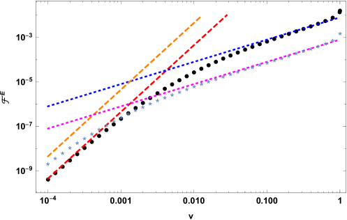
Figure 1: The numerically evaluated TE frictional force (18) [dots] compared with the low velocity approximation (21) [dashed red line]. For larger velocities, not too close to the speed of light, the force is well approximated by (24) [short-dashed blue line]. In the ultrarelativistic limit, the TE friction approaches the value (26). Here we have chosen the separation distance of the particle from the plate to be $a=100\,\mbox{nm}$, where the Drude model should be approximately valid, so for gold, $\alpha=9.0$, $\beta=0.035$. Also shown, by stars, is the friction for one-tenth the value of the dissipative parameter, $\beta=0.0035$, but with $\alpha$ unchanged, compared with the low-velocity [dashed orange] and intermediate velocity [short-dashed magenta] approximations, which exhibits the enhancement at low velocity and supression at high velocity caused by smaller dissipation.

For moderate velocities, the small $\beta$ expansion

$$f^{E}(u,\theta;\gamma;\alpha,\beta)\approx\frac{\beta}{\sqrt{\gamma^{2}-1}\cos\theta}\frac{\alpha^{2}\sin^{2}\theta}{[u+\sqrt{u^{2}+\alpha^{2}}]^{2}}\frac{1}{\sqrt{u^{2}+\alpha^{2}}},\quad\beta\ll v,$$ (22)

reproduces the approximately linear region in Fig. 1 for intermediate velocities. To see this, let $\gamma$ approach 1. The $\theta$ integral is just $\int_{0}^{2\pi}d\theta\sin^{2}\theta=\pi$ and the remaining $u$ integral is

$$I_{E}(\alpha)=\frac{1}{\alpha^{2}}\int_{0}^{\infty}du\,u\,e^{-u}\frac{(\sqrt{u^{2}+\alpha^{2}}-u)^{2}}{\sqrt{u^{2}+\alpha^{2}}},$$ (23)

which can be written in terms of Struve and Bessel functions as shown in Appendix B. In this way we obtain

$$\mathscr{F}^{E}\approx\pi\beta vI_{E}(\alpha),\quad\beta\ll v\ll 1.$$ (24)

The agreement with numerical integration is good, as also shown in Fig. 1.

Extracting the high-velocity limit is rather more subtle. If we continue to use the small $\beta$ expansion (22), we encounter the $\theta$ integral

$$\int_{0}^{2\pi}d\theta\frac{\sin^{2}\theta}{\cos^{2}\theta+\frac{1}{\gamma^{2}-1}}\approx 2\pi\gamma,\quad\gamma\gg 1.$$ (25)

In terms of the function $I_{E}(\alpha)$, the TE friction in the $\gamma\to\infty$ limit approaches

$$\mathscr{F}^{E}\sim 2\pi\beta I_{E}(\alpha),$$ (26)

twice the limit as $v\to 1$ of Eq. (24). In Fig. 2 we show that this linear behavior in $\beta$ matches the exact integration quite well for low $\beta$.

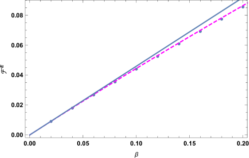
Figure 2: The linear behavior (26) in the damping parameter $\beta$ of the ultrarelativistic TE friction [upper blue line], compared with exact data [dots] for $\alpha=9.0$, $\gamma=100$. For larger values of $\beta$ the data falls below the linear curve. The curve that matches the data well [magenta, dashed] is based on the more exact treatment (27).

Note, as further shown in Appendix B, Eq. (51), that the force tends to zero as $\omega_{p}\to\infty$, as we might expect for a perfect conductor.

The astute reader might question the validity of the expansion (22) in powers of the damping parameter $\beta$, since $\cos\theta=0$ is included in the region of integration. We can test this procedure in the ultrarelativistic limit by breaking up the $\theta$ integration into two intervals, $0<\theta<\theta_{0}$, $\theta_{0}<\theta<\pi/2$, where $\pi/2-\theta_{0}\ll 1$, but $\gamma\cos\theta_{0}\gg 1$. Then the former interval is seen to give a contribution to the friction which goes like $1/\gamma$ as $\gamma\to\infty$, while the latter can be approximately written as

$$\mathscr{F}^{E}\approx 8\int_{0}^{\infty}du\,u\,e^{-u}\int_{0}^{\infty}d\phi\frac{\phi}{\phi^{2}+1}\Im\left(1+\sqrt{1+\frac{\alpha^{2}/u^{2}}{1+i\beta/(u\phi)}}\right)^{-1}.$$ (27)

Here $\phi=\gamma(\pi/2-\theta)$. Numerical integration of this is more stable than that of the original expression. Figure 2 displays the result, which matches the linear behavior for small $\beta$, and the exact data for larger values of the damping. Expanding this to first order in $\beta$, of course, yields Eq. (26).

IV TM contribution

We turn now to the dominant TM contribution, which is, in general, rather more subtle. The $v\to 0$ limit is easy, since the leading contribution in the low $v$ limit is

$$f^{H}(v,\omega)\to\frac{4\omega a}{v^{2}}\frac{\beta}{\alpha^{2}}.$$ (28)

Inserting this into the formula for the force (18) we find the low-velocity limit as given by Ref. boyer1974 :

$$\mathscr{F}^{H}=4\pi\frac{\beta}{\alpha^{2}}v,\quad\mbox{or}\quad F^{H}\sim-\frac{e^{2}}{8\pi a^{2}}\frac{\beta v}{\alpha^{2}}=-\frac{e^{2}}{16\pi}\frac{\nu v}{\omega_{p}^{2}}\frac{1}{a^{3}},\quad v\ll\beta,$$ (29)

noting that the connection between the Drude-model parameters and the Ohmic conductivity at zero frequency is $\sigma(0)=\omega_{p}^{2}/\nu$. This is much larger than the $F^{E}$ contribution given in Eq. (21). We demonstrate that this agrees with the exact numerical integration of the TM force in Fig. 3.

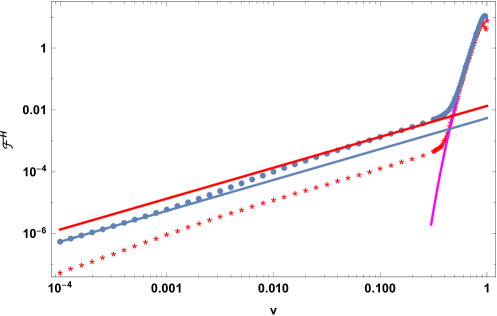
Figure 3: The dependence of the TM frictional force on velocity [dots] compared with the low velocity approximation (29) [lower, blue, straight line]. Again the parameters are $\alpha=9.0$ and $\beta=0.035$. Agreement is very good for small velocities, $v\ll\beta$. For larger velocities, the friction, computed numerically from Eq. (18), agrees well with Eq. (31) [upper, red, straight line] for intermediate velocities, $\beta\ll v\ll 1$. The high-velocity peak, for $v\sim 1$, is well reproduced by Eq.(36) [magenta curve], which approaches the asymptotic value (37), nonmonotonically, with a maximum for $v<1$. To demonstrate the effect of $\beta$, we also plot the frictional force [red stars] for $\beta=0.0035$, one-tenth the value above, but with the same plasma frequency parameter $\alpha$. For low and intermediate velocities, the friction is also reduced by a factor of 10, as expected, but the high-velocity peak is unchanged. (Instability of the numerical integration for small $\beta$ is seen at velocities near the speed of light.)

For somewhat higher velocities, $\beta\ll v\ll 1$, we can expand first in $\beta/v$, and then in $v$, and then writing $f^{H}=2\frac{\gamma^{2}}{\gamma^{2}-1}\Im\chi$, we find

$$\Im\chi=\frac{vu\beta\cos\theta}{\alpha^{2}}\sqrt{1+\frac{\alpha^{2}}{u^{2}}}\left(1-\frac{1}{2}\frac{\alpha^{2}/u^{2}}{1+\alpha^{2}/u^{2}}\right),$$ (30)

so when this is inserted into the formula (18) for $\mathscr{F}^{H}$ we obtain (see Appendix B)

$$\mathscr{F}^{H}\approx 2\pi v\beta J_{H}(\alpha),\quad J_{H}(\alpha)=\frac{1}{\alpha^{2}}\int_{0}^{\infty}du\,e^{-u}u\sqrt{u^{2}+\alpha^{2}}\left(1-\frac{1}{2}\frac{\alpha^{2}}{u^{2}+\alpha^{2}}\right),\quad\beta\ll v\ll 1.$$ (31)

This agrees closely with the linear intermediate velocity region seen in Fig. 3.

Turning to higher velocities, we note that the expansion method in $\beta$ that worked well in the TE case fails. This is because the force in this case is no longer analytic in $\beta$; the integrand in the friction develops a singularity at $\beta=0$, for sufficiently high velocities. We write Eq. (12b) exactly as

$$f^{H}=\frac{2\gamma^{2}}{\gamma^{2}-1}\Im\chi,\quad\mbox{where}\quad\chi=\left\{1+\left[1-\frac{\alpha^{2}}{u^{2}\phi^{2}}\frac{1}{1+i\beta/(u\phi)}\right]^{-1}\sqrt{1+\frac{\alpha^{2}}{u^{2}}\frac{1}{1+i\beta/(u\phi)}}\right\}^{-1},$$ (32)

with $\phi=\sqrt{\gamma^{2}-1}\cos\theta$. The TM frictional force is then

$$\mathscr{F}^{H}=\frac{8\gamma^{2}}{\sqrt{\gamma^{2}-1}}\int_{0}^{\infty}du\,u\,e^{-u}\int_{0}^{\sqrt{\gamma^{2}-1}}\frac{d\phi\,\phi}{\sqrt{\gamma^{2}-1-\phi^{2}}}\frac{1}{\phi^{2}+1}\Im\chi.$$ (33)

To get the relativistic behavior, as noted above, when $\beta=0$ the denominator in $f^{H}$ develops a pole at $\phi=\phi_{0}$, where

$$\phi^{2}_{0}=\sqrt{1+\frac{\alpha^{2}}{u^{2}}}-1.$$ (34)

So as $\beta\to 0$, we approximate $f^{H}$ by

$$f^{H}\sim\frac{2\gamma^{2}}{\gamma^{2}-1}\Im\left[\frac{u\left(\phi^{2}-\frac{\alpha^{2}}{u^{2}}\right)}{\lambda(\phi^{2}-\phi_{0}^{2})+i\epsilon}\right],\quad\lambda=u+\sqrt{u^{2}+\alpha^{2}}.$$ (35)

Here $\epsilon$ is proportional to $\beta$, is always positive, and for $\alpha\gg u$ approaches $\epsilon=\beta\sqrt{\alpha}/u^{3/2}$. Thus, for very small $\epsilon$, the imaginary part yields a $\delta$ function in $\phi$, which lies in the region of the $\phi$ integration only if $\gamma^{2}>\sqrt{1+\frac{\alpha^{2}}{u^{2}}}$. Thus, we find that Eq. (35) implies in the limit $\beta\to 0$

$$\mathscr{F}^{H}\approx\frac{4\pi\gamma}{\sqrt{\gamma^{2}-1}}\frac{1}{\alpha^{2}}\int_{\alpha/\sqrt{\gamma^{4}-1}}^{\infty}du\,u\,e^{-u}\frac{(u-\sqrt{u^{2}+\alpha^{2}})^{2}}{\sqrt{1-\frac{1}{\gamma^{2}}\sqrt{1+\frac{\alpha^{2}}{u^{2}}}}}.$$ (36)

This agrees well with the exact $\mathscr{F}^{H}$ for high velocities, is more stable numerically, and is shown in Fig. 3. The peak seen there is shown in more detail in Fig. 4.

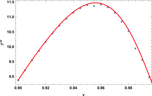
Figure 4: The TM frictional force, obtained by numerical integration, for values of $v$ for which $\mathscr{F}^{H}$ is maximum. Again we use nominal values of the plasma frequency and the damping parameter for gold, at a 100 nm separation, $\alpha=9.0$, $\beta=0.035$. The numerical data [dots], which has some instability, is fit well by Eq. (36) [continuous curve]. The maximum value is some 35% larger than the limiting value given by Eq. (37).

The dependence of this peak on $\alpha$ is shown in Fig. 5.

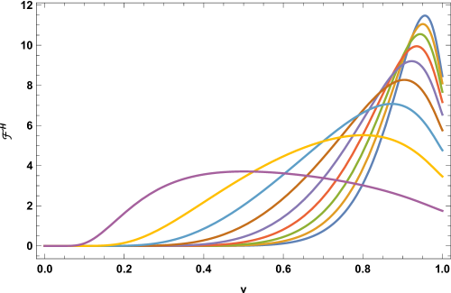
Figure 5: The function (36) for various values of $\alpha$, from $\alpha=1$ to $\alpha=9$ by unit steps, which in all cases agrees with exact numerical data for the TM (or total) frictional force. The peak shifts to lower velocities as $\alpha$ decreases, and the magnitude of the peak also decreases.

From Eq. (36) we obtain the limiting value for $\gamma\to\infty$, $\beta\to 0$:

$$\mathscr{F}^{H}\to 4\pi I_{H}(\alpha)=\frac{4\pi}{\alpha^{2}}\int_{0}^{\infty}du\,u\,e^{-u}\left(u-\sqrt{u^{2}+\alpha^{2}}\right)^{2},$$ (37)

which remarkably is not zero. See Appendix B for an explicit form for this integral. It is plotted in Fig. 7. For small $\beta$ the ultrarelativistic limit exhibits a weak dependence on the value of $\beta$, as shown in Fig. 6. This is computed by taking the $\gamma\to\infty$ limit of Eq. (33), and noting that only values of $\phi\lesssim\gamma$ are relevant:

$$\mathscr{F}^{H}\sim 8\int_{0}^{\infty}du\,u\,e^{-u}\int_{0}^{\infty}\frac{d\phi\,\phi}{\phi^{2}+1}\Im\chi.$$ (38)

As shown in Appendix B, $I_{H}(\alpha)\to 1$ as $\alpha\to\infty$. The difference between the dependencies of the frictional force on the plasma frequency shown in Fig. 7 is striking. This is correlated with the completely different dependence of the frictional force on the dissipation parameter $\beta$. Indeed, in the high-velocity, large-plasma-frequency limit,

$$\frac{\mathscr{F}^{E}}{\mathscr{F}^{H}}\to\frac{\beta}{2\alpha},\quad\gamma\to\infty,\,\alpha\to\infty.$$ (39)

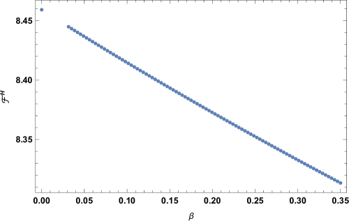
Figure 6: The TM frictional force in the $\gamma\to\infty$ limit for $\alpha=9$ as a function of $\beta$. Note there is a mild linear dependence on the damping parameter $\beta$, and that the force tends to a nonzero value for $\beta\to 0+$. (The numerical integral becomes unstable for small values of $\beta$, but the limiting value (37) at $\beta=0$ is shown.)

V Conclusions

In this paper we have reconsidered classical friction between a charged particle and an imperfectly conducting plate. We describe the latter by the Drude model. Only the nonrelativistic regime had been considered previously, to our knowledge. We examine both the TE mode, which is quite negligible in practice, and the TM mode. The low velocity limit is very straightforward to analyze, but the limit of high velocities (ultrarelativistic) is considerably more subtle. We obtain results for all velocities by a combination of analytic and numerical techniques.

The difference between the TE force seen in Fig. 1 and the TM force seen in Fig. 3, is remarkable. Not only is the value of the TE force typically orders of magnitude smaller, but the TM force is nonmonotonic in the velocity. It may seem surprising that the maximum of the frictional force occurs for an intermediate value of the velocity, as shown in more detail in Fig. 4, but this is due to the appearance of a pole in the integrand for small damping.

How big are these effects, and might they be experimentally measurable? We compare the largest value of the TM friction, $\mathscr{F}^{H}\approx 11.4$, with our parameters, from Fig. 3, with the force on a static charged particle next to a conducting plate, $F_{c}=-e^{2}/(16\pi a^{2})$. For our nominal values $\alpha=9$, $\beta=0.035$, the ratio is maximum at about 0.96 times the speed of light:

$$\frac{F}{F_{c}}\leq 1.81.$$ (40)

This should be readily observable. This ratio drops to about 1.33 for an ultrarelativistic charged particle.

Appendix A Electromagnetic Green’s Function

Maxwell’s equations in a medium characterized by position- and frequency-dependent permittivity $\varepsilon$ and permeability $\mu$ yield the wave equation for the electric field

$$\bm{\nabla}\times\frac{1}{\mu}\bm{\nabla}\times\mathbf{E}-\omega^{2}\varepsilon\mathbf{E}=i\omega\mathbf{j},$$ (41)

where $\mathbf{E}=\mathbf{E}(\mathbf{r};\omega)$, $\mathbf{j}=\mathbf{j}(\mathbf{r};\omega)$. The electromagnetic Green’s dyadic satisfies a similar equation,

$$\left[\frac{1}{\omega^{2}}\bm{\nabla}\times\frac{1}{\mu}\bm{\nabla}\times-\varepsilon\right]\bm{\Gamma}(\mathbf{r,r^{\prime}};\omega)=\bm{1}\delta(\mathbf{r-r^{\prime}}).$$ (42)

From this Eq. (2) immediately follows.

For the planar geometry we are considering for the dielectric slab, the Green’s dyadic possesses translational invariance in the plane of the slab, the $x$-$y$ plane, so we have the Fourier representation (4), where, in a coordinate system in which $\mathbf{k_{\perp}}$ lies in the $x$ direction, $\mathbf{g}$ breaks up into block-diagonal form:

$$\mathbf{g}(z,z^{\prime};\mathbf{k_{\perp}},\omega)=\left(\begin{array}[]{ccc}\frac{1}{\varepsilon}\partial_{z}\frac{1}{\varepsilon^{\prime}}\partial_{z^{\prime}}g^{H}-\frac{1}{\varepsilon}\delta(z-z^{\prime})&0&\frac{ik}{\varepsilon\varepsilon^{\prime}}\partial_{z}g^{H}\\ 0&\omega^{2}g^{E}&0\\ -\frac{ik}{\varepsilon\varepsilon^{\prime}}\partial_{z^{\prime}}g^{H}&0&\frac{k^{2}}{\varepsilon\varepsilon^{\prime}}g^{H}-\frac{1}{\varepsilon}\delta(z-z^{\prime})\end{array}\right).$$ (43)

Here $\varepsilon=\varepsilon(z)$, $\varepsilon^{\prime}=\varepsilon(z^{\prime})$, $k=|\mathbf{k}_{\perp}|$, and $g^{E}(z,z^{\prime})$, $g^{H}(z,z^{\prime})$ are the transverse electric and transverse magnetic Green’s functions, which satisfy [in a general medium with both permittivity $\varepsilon=\varepsilon(z,\omega)$ and permeability $\mu=\mu(z,\omega)$]

$$\left(-\frac{\partial}{\partial z}\frac{1}{\mu}\frac{\partial}{\partial z}+\frac{k^{2}}{\mu}-\omega^{2}\varepsilon\right)g^{E}(z,z^{\prime}) = \delta(z-z^{\prime}),$$ (44a)

$$\left(-\frac{\partial}{\partial z}\frac{1}{\varepsilon}\frac{\partial}{\partial z}+\frac{k^{2}}{\varepsilon}-\omega^{2}\mu\right)g^{H}(z,z^{\prime}) = \delta(z-z^{\prime}).$$ (44b)

For the case of a homogeneous dielectric slab extending over the half-space $z<0$, the solution of these equations for $z>0$ is given in terms of reflection coefficients by Eq. (7), as shown in textbooks, for example Ref. ce . The $\delta$-function terms in Eq. (43) are to be omitted, as “contact terms,” because we always take the coincident point limit.

For the application here, we have to remove the restriction that $\mathbf{k_{\perp}}$ lie along the $x$ axis, which we do by the orthogonal transformation

$$\mathbf{\tilde{g}}=\mathbf{O}\mathbf{g}\mathbf{O}^{T},\quad\mathbf{O}=\left(\begin{array}[]{ccc}\frac{k_{x}}{k}&-\frac{k_{y}}{k}&0\\ \frac{k_{y}}{k}&\frac{k_{x}}{k}&0\\ 0&0&1\end{array}\right).$$ (45)

Equation (6) now follows.

Appendix B Evaluation of Integrals

It is straightforward to show that the integrals occurring in the ultrarelativistic limit ($v\to 1$) for $\mathscr{F}^{E}$

$$I_{E}(\alpha)=\alpha^{2}\int_{0}^{\infty}du\,e^{-u}\frac{u}{\sqrt{u^{2}+\alpha^{2}}\left(u+\sqrt{u^{2}+\alpha^{2}}\right)^{\!2}}$$ (46a)

and in the ultrarelativistic limit for $$\mathscr{F}^{H}$$

$$I_{H}(\alpha)=\alpha^{2}\int_{0}^{\infty}du\,e^{-u}\frac{u}{\left(u+\sqrt{u^{2}+\alpha^{2}}\right)^{\!2}}$$ (46b)

may be expressed in terms of Struve and Bessel functions by using gs

$$\int_{0}^{\infty}du\,e^{-u}\left(u^{2}+\alpha^{2}\right)^{\nu-1}=\frac{\sqrt{\pi}}{2}\,(2\alpha)^{\nu-\frac{1}{2}}\,\Gamma(\nu)\left[\mathbf{H}_{\nu-\frac{1}{2}}(\alpha)-Y_{\nu-\frac{1}{2}}(\alpha)\right].$$ (47)

Thus,

$$I_{E}(\alpha) = \frac{1}{\alpha^{2}}\int_{0}^{\infty}du\,e^{-u}\,\frac{u\left(u-\sqrt{u^{2}+\alpha^{2}}\right)^{\!2}}{\sqrt{u^{2}+\alpha^{2}}}$$ (48a)

$$= \frac{1}{\alpha^{2}}\int_{0}^{\infty}du\,e^{-u}\,\frac{\left(-\alpha^{2}u+2u(u^{2}+\alpha^{2})-2u^{2}\sqrt{u^{2}+\alpha^{2}}\right)}{\sqrt{u^{2}+\alpha^{2}}}$$

$$= \frac{1}{\alpha^{2}}\int_{0}^{\infty}du\,e^{-u}\left(-\alpha^{2}\,\frac{d}{du}\sqrt{u^{2}+\alpha^{2}}+\frac{2}{3}\,\frac{d}{du}\left(u^{2}+\alpha^{2}\right)^{\!\frac{3}{2}}-2u^{2}\right)$$

$$= \frac{1}{\alpha^{2}}\left[\frac{\alpha^{3}}{3}+\int_{0}^{\infty}du\,e^{-u}\left(-\alpha^{2}\sqrt{u^{2}+\alpha^{2}}+\frac{2}{3}\left(u^{2}+\alpha^{2}\right)^{\!\frac{3}{2}}-2u^{2}\right)\right]$$

$$= -\frac{4}{\alpha^{2}}+\frac{\alpha}{3}-\frac{\pi\alpha}{2}\left[\mathbf{H}_{1}(\alpha)-Y_{1}(\alpha)\right]+\pi\left[\mathbf{H}_{2}(\alpha)-Y_{2}(\alpha)\right].$$

Likewise,

$$I_{H}(\alpha) = \frac{1}{\alpha^{2}}\int_{0}^{\infty}du\,e^{-u}\,u\left(u-\sqrt{u^{2}+\alpha^{2}}\right)^{\!2}$$ (48b)

$$= \frac{1}{\alpha^{2}}\int_{0}^{\infty}du\,e^{-u}\left(\alpha^{2}u+2u^{3}+2\alpha^{2}\sqrt{u^{2}+\alpha^{2}}-2\left(u^{2}+\alpha^{2}\right)^{\!\frac{3}{2}}\right)$$

$$= \frac{12}{\alpha^{2}}+1+\pi\alpha\left[\mathbf{H}_{1}(\alpha)-Y_{1}(\alpha)\right]-3\pi\left[\mathbf{H}_{2}(\alpha)-Y_{2}(\alpha)\right].$$

For small values of $\alpha$, standard expansions of $\mathbf{H}_{n}(\alpha)$ and $Y_{n}(\alpha)$ may be used to evaluate these functions:

$$I_{E} \sim \frac{\alpha}{3}-\frac{\alpha^{2}}{16}\left(1-4\gamma_{E}-4\ln\frac{\alpha}{2}\right)-\frac{1}{5}\alpha^{3}+\dots,$$ (49a)

$$I_{H} \sim -\frac{\alpha^{2}}{16}\left(1+4\gamma_{E}+4\ln\frac{\alpha}{2}\right)+\frac{4}{15}\alpha^{3}+\dots,$$ (49b)

for $\alpha\ll 1$, in terms of Euler’s constant, $\gamma_{E}=0.57721\dots$. For large values of $\alpha$, the following asymptotic expansion gs may be employed:

$$\mathbf{H}_{n}(\alpha)-Y_{n}(\alpha)=\frac{1}{\pi}\sum_{m=0}^{p-1}\frac{\Gamma\left(m+\frac{1}{2}\right)}{\Gamma\left(n+\frac{1}{2}-m\right)}\left(\frac{\alpha}{2}\right)^{\!n-1-2m}+O\left(\alpha^{n-1-2p}\right).$$ (50)

It follows that

$$I_{E}\sim\frac{1}{\alpha}-\frac{4}{\alpha^{2}},\quad I_{H}\sim 1-\frac{4}{\alpha},\quad\mbox{as}\quad\alpha\to\infty.$$ (51)

These functions are plotted in Fig. 7.

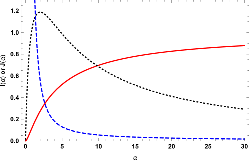
Figure 7: Behavior of the integrals $I_{H,E}$ as functions of the plasma frequency parameter $\alpha$. The TE contribution [black, dotted] $I_{E}$ is multiplied by a factor of 10, so the two functions may be shown on the same graph. The TM integral $I_{H}$ is shown by the solid red curve. These functions describe the high-velocity limit of the frictional force, according to Eqs. (26) and (37). Also plotted is the function $J_{H}(\alpha)$ [dashed, blue, curve], which describes the intermediate-velocity dependence of the TM frictional force, according to Eq. (31).

$I_{E}(\alpha)$ also describes the behavior of $\mathscr{F}^{E}$ for intermediate velocities, according to Eq. (24), while the corresponding intermediate-velocity behavior of $\mathscr{F}^{H}$ is given by Eq. (31) in terms of $J_{H}(\alpha)$, where

$$J_{H}(\alpha) = \frac{1}{\alpha^{2}}\int_{0}^{\infty}du\,e^{-u}u\sqrt{u^{2}+\alpha^{2}}\left(1-\frac{1}{2}\frac{\alpha^{2}}{u^{2}+\alpha^{2}}\right)$$ (52)

$$= \frac{\alpha}{6}+\frac{\pi}{2}\left(\mathbf{H}_{2}(\alpha)-Y_{2}(\alpha)\right)-\frac{\alpha\pi}{4}\left(\mathbf{H}_{1}(\alpha)-Y_{1}(\alpha)\right).$$

This is also plotted in Fig. 7. The behaviors for large and small values of $\alpha$ are

$$J_{H}(\alpha) \sim \frac{2}{\alpha^{2}}+\frac{\alpha}{6}+\frac{\alpha^{2}}{32}\left(-1+4\gamma_{E}+4\ln\frac{\alpha}{2}\right),\quad\alpha\ll 1,$$ (53a)

$$\sim \frac{1}{2\alpha}+\frac{9}{2\alpha^{3}},\quad\alpha\gg 1.$$ (53b)

Appendix C Vavilov-Čerenkov Radiation

To illustrate the further utility of our Green’s function approach, we apply Eqs. (5) and (6) to the situation of a charged particle moving through a homogeneous nondissipative dielectric material faster than the speed of light in the medium, $1/n=1/\sqrt{\varepsilon}$. In this case we will disregard dissipation in the material, setting $\nu=0$; the imaginary part comes from the region of frequencies where $v>1/n(\omega)$. The TE part of the drag on the particle is given by

$$F^{E}=-\frac{e^{2}}{2\pi}\int\frac{d\omega}{\omega}\int_{-\infty}^{\infty}\frac{dk_{y}}{2\pi}\frac{\omega^{2}}{k_{y}^{2}+\omega^{2}/v^{2}}k_{y}^{2}\,\Im\frac{1}{2\kappa^{\prime}},$$ (54)

since we now only have the bulk (first) term in Eq. (7), except that the particle is in the medium, so $1/(2\kappa)\to 1/(2\kappa^{\prime})$. The branch line is chosen to run between the two branch points, where $k_{y}^{2}=n(\omega)^{2}\omega^{2}[1-1/(n(\omega)^{2}v^{2})]$, on the real $k_{y}$ axis, The subtlety is the sign of the imaginary part. This is resolved by noting that the retarded Green’s function must have singularities only in the lower-half $\omega$ plane, which is consistent with the requirement that, in the case of infinitesimal damping, $n(\omega)^{2}\omega^{2}$ has an imaginary part $\epsilon\operatorname{sgn}(\omega)$, with $\epsilon\to 0+$. Therefore, the $k_{y}$ integration passes below the branch line for $\omega>0$, and above for $\omega<0$. In dimensionless form, that integral then is

$$\int_{-1}^{1}dx\frac{x^{2}}{x^{2}+a^{2}}\frac{\operatorname{sgn}{\omega}}{\sqrt{1-x^{2}}}=\pi\operatorname{sgn}(\omega)\left(1-\frac{a}{\sqrt{1+a^{2}}}\right),$$ (55)

with $a=\left(vn(\omega)\sqrt{1-1/(vn(\omega))^{2}}\right)^{-1}$, so that the above integral is simply $\operatorname{sgn}(\omega)\pi[1-1/(vn(\omega))]$. The resulting drag force due to Čerenkov radiation is

$$F^{E}=-\frac{e^{2}}{8\pi}\int d\omega\,|\omega|\left(1-\frac{1}{n(\omega)v}\right),$$ (56)

where the integral is over the region where $n(\omega)>1/v$.

The TM contribution to the drag force is

$$F^{H}=\frac{e^{2}}{2\pi}\int\frac{d\omega}{\omega}\int_{-\infty}^{\infty}\frac{dk_{y}}{2\pi}\frac{\omega^{2}/v^{2}}{k_{y}^{2}+\omega^{2}/v^{2}}\Im\left[\frac{\kappa^{\prime 2}}{\varepsilon(\omega)^{2}}\frac{\varepsilon(\omega)}{2\kappa^{\prime}}\right],$$ (57)

because except in the exponent, the TM Green’s function is obtained from that for TE by the replacement $\kappa^{\prime}\to\kappa^{\prime}/\varepsilon$. After doing the $k_{y}$ integral as above, which now is

$$-\operatorname{sgn}(\omega)\int_{-1}^{1}dx\frac{\sqrt{1-x^{2}}}{x^{2}+a^{2}}=\pi\operatorname{sgn}(\omega)\left(1-vn(\omega)\right),$$ (58)

we have

$$F^{H}=-\frac{e^{2}}{8\pi}\int d\omega\,|\omega|\frac{1}{n(\omega)v}\left(1-\frac{1}{n(\omega)v}\right).$$ (59)

Adding the two modes together,

$$F=F^{E}+F^{H}=-\frac{e^{2}}{4\pi}\int d\omega\,\omega\left(1-\frac{1}{n(\omega)^{2}v^{2}}\right),$$ (60)

where now the integration is over positive frequencies for which the speed of the particle exceeds that of light in the medium, $1/n(\omega)$. This formula exactly coincides with the energy loss rate found in Eq. (36.19) of Ref. ce due to the energy radiated by Vavilov-Čerenkov effect. (Note, Gaussian units were used there, and $e_{\rm HL}^{2}=4\pi e_{\rm G}^{2}$.)

References

(1)
K. A. Milton, J. S. Høye and I. Brevik,
“The reality of Casimir friction,”
Symmetry 8, no. 5, 29 (2016)
doi:10.3390/sym8050029
[arXiv:1508.00626 [quant-ph]].
(2)
T. H. Boyer,
“Penetration of the electric and magnetic velocity fields of a nonrelativistic
point charge into a conducting plane,”
Phys. Rev. A 9, 68–82 (1974).
(3)
T. H. Boyer,
“Penetration of electromagnetic velocity fields through a conducting wall of
finite thickness,”
Phys. Rev. E 53, 6450–6459 (1996).
(4)
M. S. Tomassone and A. Widom,
“Electronic friction forces on molecules moving near metals,”
Phys. Rev. B 56, 4938–4943 (1997).
(5)
M. S. Tomassone and A. Widom,
“Friction forces on charges moving outside of a conductor due to Ohm’s law
heating inside of a conductor,”
Am. J. Phys. 65, 1181–1183 (1997).
(6)
J. B. Sokoloff, “Kinetic friction due to Ohm’s law heating,”
J. Phys.: Condens. Matter 14, 5277–5287 (2002).
(7)
A. Dayo, W. Alnasrallah, and J. Krim, “Superconductivity-dependent
sliding friction,” Phys. Rev. Lett. 80, 1690–1693 (1998).
(8)
R. L. Renner, J. E. Rutledge, and P. Taborek, “Quartz microbalance
studies of superconductivity-dependent sliding friction,” Phys. Rev. Lett. 83, 1261 (1999).
(9)
J. Krim, “Krim replies,” Phys. Rev. Lett. 83, 1262 (1999).
(10)
B. N. J. Persson, “Electronic friction on a superconducting surface,”
Solid State Comm. 115, 145–148 (2000).
(11)
R. L. Olmon, B. Slovik, T. W. Johnson, D. Shelton, S.-H. Oh, G. D. Boreman,
and M. B. Raschke, “Optical dielectric function of gold,” Phys. Rev. B 86, 235147 (2012).
(12)
J. Schwinger, L. L. DeRaad, Jr. and K. A. Milton,
“Casimir effect in dielectrics,”
Ann. Phys. (N.Y.) 115, 1–23 (1979).
doi:10.1016/0003-4916(78)90172-0
(13)
J. Schwinger, L. L. DeRaad, Jr., K. A. Milton, and W.-y. Tsai,
Classical Electrodynamics (Perseus, New York, 1998).
(14)
I. Brevik and J. B. Aarseth,
“Temperature dependence of the Casimir effect,”
J. Phys. A 39, 6187–6193 (2006)
[arXiv:quant-ph/0511037](Proc. 7th Workshop
on Quantum Field Theory Under the Influence of External Conditions,
Barcelona 5–9 September 2005, ed. E. Elizalde)
(15)
I. S. Gradshteyn, I. M. Ryzhik, Y. Y. Geronimus,
M. Y. Tseytlin, A. Jeffrey. D. Zwillinger, V. H. Moll, (eds.),
Table of Integrals, Series, and Products. Translated by Scripta Technica,
Inc. (8 ed.).
Academic Press, Inc. ISBN 978-0-12-384933-5.