Deep Learning in Wide-field Surveys: Fast Analysis of Strong Lenses in Ground-based Cosmic Experiments

Abstract

Searches and analyses of strong gravitational lenses are challenging due to the rarity and image complexity of these astronomical objects. Next-generation surveys (both ground- and space-based) will provide more opportunities to derive science from these objects, but only if they can be analyzed on realistic time-scales. Currently, these analyses are expensive. In this work, we present a regression analysis with uncertainty estimates using deep learning models to measure four parameters of strong gravitational lenses in simulated Dark Energy Survey data. Using only $gri$-band images, we predict Einstein Radius ($\theta_{\rm E}$), lens velocity dispersion ($\sigma_{\rm v}$), lens redshift ($z_{\rm l}$) to within $10-15\%$ of truth values and source redshift ($z_{\rm s}$) to $30\%$ of truth values, along with predictive uncertainties. This work helps to take a step along the path of faster analyses of strong lenses with deep learning frameworks.

1 Introduction

Strong gravitational lensing occurs when massive objects (e.g., galaxies and their dark matter haloes) deform spacetime, deflecting the light rays that originate at sources along the line of sight to the observer (e.g., Schneider et al., 2013; Petters et al., 2012; Mollerach and Roulet, 2002). The key signature of a strong lens is a magnified and multiply imaged or distorted image of the background source, which can only occur if the source is sufficiently closely aligned to the line of sight of the warped gravitational potential generated by the lensing mass. Strong lensing also depends on the angular diameter distances between observer, lens, and source, which encloses information about the underlying cosmology. The source light may be magnified up to a hundred times, as the light deflection due to strong lensing conserves the surface brightness while increasing the total angular size of the object.

Strong lensing systems are unique probes of many astrophysical and cosmological phenomena. They act as “gravitational telescopes,” enabling the study of distant source objects that would be otherwise too faint to observe, such as high redshift galaxies (e.g., Ebeling et al., 2018; Richard et al., 2011; Jones et al., 2010): dwarf galaxies (Marshall et al., 2007), star-forming galaxies (Stark et al., 2008), quasar accretion disks (Poindexter et al., 2008), and faint Lyman-alpha blobs (Caminha et al., 2015). Lensing systems can also be used as non-dynamical probes of the mass distribution of galaxies (e.g. Treu and Koopmans, 2002, 2002; Koopmans et al., 2006a), and galaxy clusters (e.g., Kovner, 1989; Abdelsalam et al., 1998; Natarajan et al., 2007; Zackrisson and Riehm, 2010; Carrasco et al., 2010; Coe et al., 2010), providing a key observational window on dark matter (see, e.g., Meneghetti et al., 2004).

Strong lensing has also been used — alone or in combination with other probes — to derive cosmological constraints on the cosmic expansion history, dark energy, and dark matter (see, e.g., Jullo et al., 2010; Caminha et al., 2016; Bartelmann et al., 1998; Cooray, 1999; Golse et al., 2002; Treu and Koopmans, 2002; Yamamoto et al., 2001; Meneghetti et al., 2004, 2005; Jullo et al., 2010; Magaña et al., 2015; Cao et al., 2015; Caminha et al., 2016; Schwab et al., 2010; Enander and Mörtsell, 2013; Pizzuti et al., 2016). Precise and accurate time-delay distance measurements of multiply-imaged lensed QSO systems have been used to measure the expansion rate of the universe (Oguri, 2007; Suyu et al., 2010). More recently, this technique has also been applied to multiply-imaged lensed supernovae (Kelly et al., 2015; Goobar et al., 2016). Strong lensing can also be used to constrain dark matter models (Vegetti et al., 2012; Hezaveh et al., 2014; Gilman et al., 2018; Rivero et al., 2018; Bayer et al., 2018), as well as detect dark-matter substructures along the line-of-sight (Despali et al., 2018; McCully et al., 2017).

The broad range of applications has inspired many searches for strong lensing systems. Many of these searches have been carried out on high-quality space-based data from the Hubble Space Telescope (HST): Hubble Deep Field (HDF; Hogg et al., 1996), the HST Medium Deep Survey (Ratnatunga et al., 1999), the Great Observatories Origins Deep Survey (GOODS; Fassnacht et al., 2004), the HST Archive Galaxy-scale Gravitational Lens Survey (HAGGLeS; Marshall, 2009), the Extended Groth Strip (EGS; Marshall et al., 2009), and the HST Cosmic Evolution survey (COSMOS; Faure et al., 2008; Jackson, 2008).

However, there is also a plethora of ground-based imaging data that merits exploration. The majority of confirmed strong lensing systems that have been identified to-date were first discovered in ground-based surveys, such as the Red-Sequence Cluster Survey (RCS; Gladders et al., 2003; Bayliss, 2012), the Sloan Digital Sky Survey (SDSS; Estrada et al., 2007; Belokurov et al., 2009; Kubo et al., 2010; Wen et al., 2011; Bayliss, 2012), the Deep Lens Survey (DLS; Kubo and Dell’Antonio, 2008), The Canada-France-Hawaii Telescope (CFHT) Legacy Survey (CFHTLS; Cabanac et al., 2007; More et al., 2012; Maturi et al., 2014; Gavazzi et al., 2014; More et al., 2016; Paraficz et al., 2016), the Dark Energy Survey (DES; e.g., Nord et al., 2015), the Kilo Degree Survey (KIDS; e.g., Petrillo et al., 2017). Also, some Strong Lensing systems were firstly detected by Hershel Space observatory and South Pole Telescope (SPT) and later followed up by ALMA (Vieira et al., 2010; Hezaveh et al., 2013; Oliver et al., 2012; Dye et al., 2018; Eales et al., 2010). Strong lenses have also been discovered in follow-up observations of galaxy clusters (e.g., Luppino et al., 1999; Zaritsky and Gonzalez, 2003; Hennawi et al., 2008; Kausch et al., 2010; Furlanetto et al., 2013) and galaxies (e.g., Willis et al., 2006). Next-generation surveys like LSST (Ivezić et al., 2008), Euclid (Laureijs et al., 2011), and WFIRST (Green et al., 2012), are projected to discover up to two orders of magnitude more lenses than what is currently known (Collett, 2015a).

Many of the current catalogs of strongs lensing systems were found through visual searches. However, the increasingly large data sets from current and future wide-field surveys necessitates the development and deployment of automated search methods to find and classify lens candidates. Neural networks are one class of automated techniques. A number of recent works have demonstrated that both traditional neural networks (Bom et al., 2017; Estrada et al., 2007) and deep neural networks (Petrillo et al., 2019b; Jacobs et al., 2019; Petrillo et al., 2019a; Metcalf et al., 2018; Lanusse et al., 2018; Glazebrook et al., 2017) can be used to identify morphological features in raw images that distinguish lenses from non-lenses, with minimal intervention from humans.

In addition to finding catalogs of lenses, inferring the properties of lenses, like the Einstein Radius or the velocity dispersion of the lensing galaxy, typically require follow-up observations as well as modeling. Conventionally, modeling is performed with computationally expensive maximum likelihood algorithms (e.g., Bradač et al., 2009; Diego et al., 2005; Coe et al., 2008; Oguri, 2010; Jullo et al., 2007; Metcalf and Petkova, 2014; Petkova et al., 2014), which can take up to weeks on CPUs and require manual input. This is a relevant limitation for statistical studies of strong lenses or even for selecting systems to follow-up on. Recently, Hezaveh et al. (2017) showed that deep learning techniques could also be used in a regression task to produce fast measurements of strong lenses: the lens parameters in that work were measured on a set of high-quality HST simulations and images. Additionally, Levasseur et al. (2017) produced uncertainty estimates on strong lensing parameters using dropout techniques, which evaluates the deep neural network from a Bayesian perspective (Gal and Ghahramani, 2016). The same approach was used by Morningstar et al. (2018) to derive uncertainties in the parameters of strong gravitational lenses from interferometric observations.

In this work, we address the problem of strong lensing analysis in ground-based wide-field astronomical surveys, which have lower image quality than space-based data. To develop and validate our deep neural network model, we produced a simulated catalog of strong lensing systems with DES-quality imaging. These simulations are used to train and evaluate the deep neural network model. The model is then used to infer the velocity dispersion $\sigma_{v}$, lens redshift $z_{l}$, source redshift $z_{s}$ and Einstein Radius $\theta_{E}$ of the lens. Our approach is generic: although the model is optimized for galaxy-scale lens systems (i.e., two objects, often visually blended, distorted image source, ring-like images or multiples images from the same source), it could be extended and optimized to analyze other species of strong lenses such as time-delay and double-source-plane systems.

This paper is organized as follows: First, in §2, we introduce the deep learning models and uncertainty estimation formalism used in this work. Then, in §3, we describe the simulated data used in this work. Following that, in §4, we describe how we trained the deep neural network model. In §5, we apply our model to a test set and evaluate its performance. Finally, we conclude and present an outlook for future work in §6.

2 Regression with Uncertainty Measurements in deep learning Models

Deep learning algorithms (Goodfellow et al., 2016; LeCun et al., 2015), and in particular Convolutional neural networks (CNNs; LeCun et al., 1998), are established as the state of art for many sectors in computer vision research (see, e.g. Russakovsky et al., 2015; Zhang et al., 2018; Lin et al., 2018; John et al., 2015; Peralta et al., 2018). In some cases, they have been shown to perform better than humans (e.g., He et al., 2015; Metcalf et al., 2018). Deep learning allows the development of algorithms that can process complex and minimally processed (even raw) data from a wide variety of sources to extract relevant features which can be effectively linked to other properties of interest. For example, in computer vision tasks, it has been successfully applied to facial recognition (Lu et al., 2017a), speech detection and characterization (Vecchiotti et al., 2018; Abdel-Hamid et al., 2014), music classification (Choi et al., 2017), medical prognostics (Li et al., 2018b) and diagnostics (Hannun et al., 2019).

Deep learning models are not restricted to solve classification tasks, i.e. discrete-variable problems. Indeed, the the universal approximation theorem (Csáji, 2001; Goodfellow et al., 2016; Hornik, 1991; Hanin, 2017; Yarotsky, 2018) states that a feed-forward neural network with a single hidden layer (depth-2) with a suitable activation function can approximate a wide variety of continuous functions on compact subsets of $R^{n}$. In this case, the layer can be infeasibly large (wide). Recently, (Lu et al., 2017b) explored the width-bounded and depth-unbounded networks in which the authors argue that a width-$n+4$, where $n$ is the size of input layers with ReLU activation functions can approximate any Lebesgue integrable function on $n$-dimensional input space. In both scenarios, depth-bounded or width-bounded, these results do not make statements on how this neural network can be trained. Nevertheless, deep learning models have been successfully applied to estimate continuous variables, i.e. to perform a regression task (Lathuilière et al., 2018a, b; Belagiannis et al., 2015).

Regression problems can be formulated as a classification problem (Rothe et al., 2018; Rogez et al., 2017) if one discretizes the output parameters. For example, in deep learning for astronomy this approach has been recently applied to photometric redshift estimation (Pasquet et al., 2019). In that work, the algorithm predicts a set of parameters that represent the probability on each bin of the photometric redshift, which allows one to derive a probability density function (PDF).

However, this procedure faces several disadvantages. For example, the maximum precision of the probability peak region is limited by the bin size.There is also a trade-off between the complexity and accuracy of the problem. In this scenario, during the optimization process, a high score in a bin next to the true value might have the same cost of a high score in a bin far from the true value. More sophisticated approaches can include multiple stages for deep regression, applying clustering, pseudo-labelling (Liu et al., 2016), or robust regression in which a probabilistic model, like Gaussian-uniform mixture, is added to make the model less sensitive to outliers (Lathuilière et al., 2018b). Most of these models are usually very specialized and non-trivial to adapt for different sets of regression problems.

In this work, we use a more direct and generic approach to adapt a typical classification deep learning model to the task of regression. We use an architecture based on the inception module (Szegedy et al., 2015, 2016). Furthermore, in order to estimate uncertainties we apply the concrete dropout technique to approximate the PDF of the estimated values. Both the model architecture and the error estimations are detailed in next subsections.

2.1 Model Architecture: Inception

Overly large neural network architectures pose a number of challenges in the training process. First, overfitting becomes a major limitation when the number of training samples do not scale as the number of parameters. Additionally, a uniform increase in the number of filters in convolutional layers requires a quadratic increase in computation. Moreover, when new layers are added to large linear architectures, many weights become close to zero and most of the computation time is not fruitful (Szegedy et al., 2015).

The inception module (shown in Fig. 2) provides a non-linear architecture, as well as sparsity in the weights. The sparsity adds a relevant advantage by making the neural network more adaptable and stable. Additionally, a wider layer increases cardinality (Tishby and Zaslavsky, 2015; Xie et al., 2017), i.e., the number of independent paths which can provide a new way of adjusting the model. With just thousands of parameters, the Inception module has been shown to outperform the traditional linear Visual Geometry Group Network (VGG; Simonyan and Zisserman, 2014) models that have tens of millions of parameters. Samples with objects of a variety of sizes present challenges for networks that lack the flexibility to contend with this. Inception does not require a prescription for the optimal convolutional kernel size, because the convolutions are performed in parallel, each with a different kernel size.

In Fig. 1, we present the Inception architecture used in this work. Starting with the original architecture (Szegedy et al., 2015), we replace the regular multi-class softmax activation function (Krizhevsky et al., 2012) after the last dense layer with an unbounded linear activation that is able to output a single continuous value — enabling the regression task. It has three streams: the input, the core, and the output. The input stream reduces dimensionality. It is composed of two consecutive blocks of 2D convolutional layers, a batch normalization layer, a ReLU activation, and 2D max pooling layers. Both convolutional layers have a kernel size of $\left(5,5\right)$, while the pooling layers have a size of $\left(2,2\right)$.

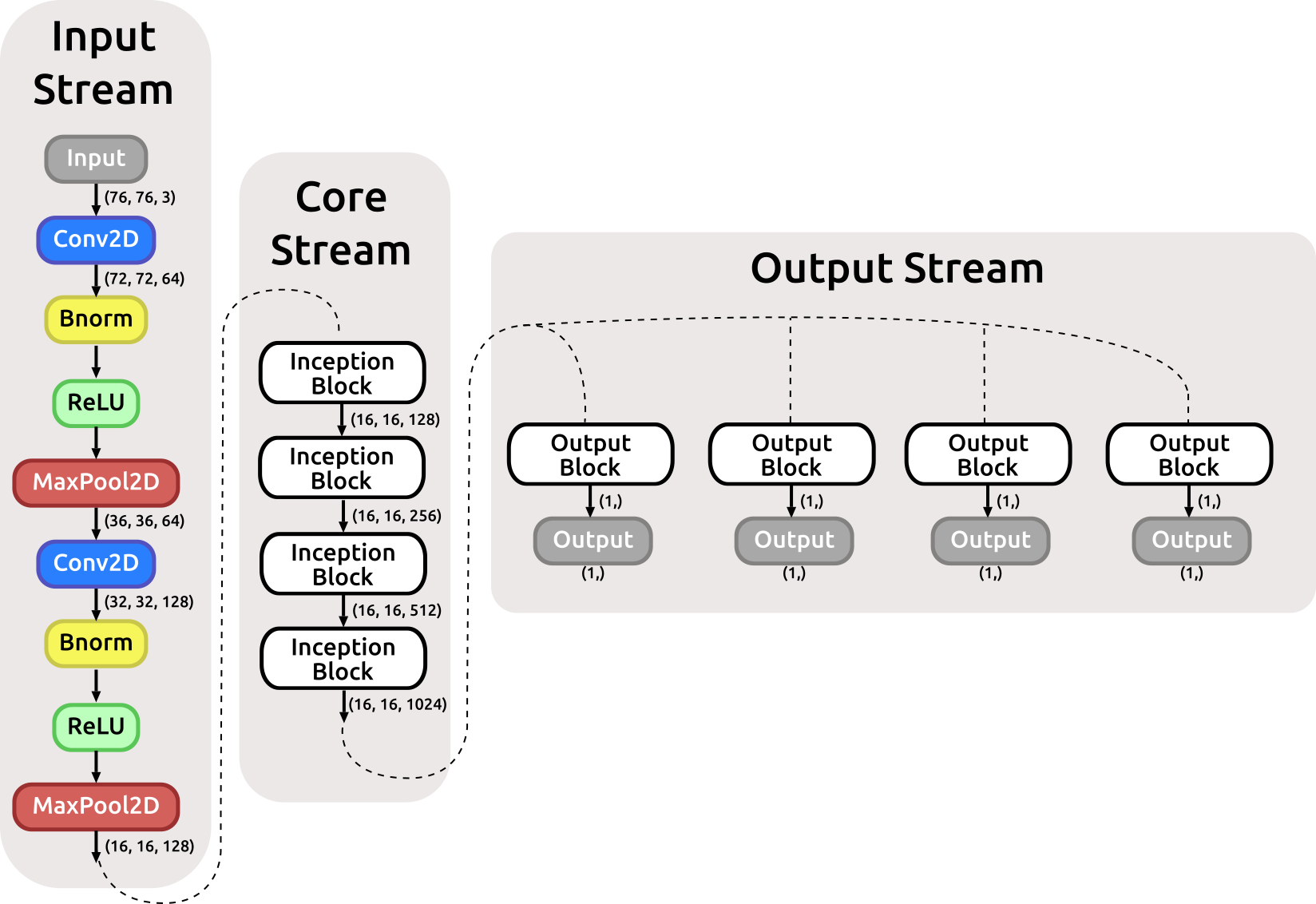
Figure 1: Diagram of the Inception network used in this work. This architecture is composed of a total of 86 layers ( convolutional, batch normalization, ReLU activations, max pooling, and dense). The size of the activation maps is shown at relevant locations of the net (after each layer that changes its size). The architecture is divided into three main streams: the input stream, which is used to reduce dimensionality of input data and optimize training; the core stream, whose main purpose is to extract meaningful spatial features from the input data; and an output stream, which correlates these extracted features with each lensing property to be estimated (see Fig. 3).

The core stream is composed of four consecutive Inception blocks. Each one of these blocks, whose structure can be seen in Fig. 2, has four branches, each with a different kernel size. The $\left(1,1\right)$ convolutions (the first convolutional layer appearing on each branch) are used for image depth reduction — i.e., to lower computational cost. Any immediately following convolutional layer has a size of $\left(3,3\right)$.

As shown in Fig. 1, apart from its depth, the size of the internal activation maps inside the core stream is not modified. Other types of architectures need to reduce activation map dimensions to extract features at different scales. However, inception modules are expected to behave this way, keeping the dimensions of activation maps, as the features at different scales are extracted using the parallel convolutional schema as mentioned earlier.

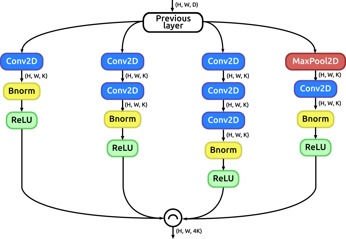
Figure 2: Diagram of the Inception block used in the Inception net, which is shown in Figure 1. This block is based on the inception module proposed by Szegedy et al. (2016) for the Inception-v2 architecture. This block allows the net to process data using different sizes of kernels, which is useful to enhance data features at different scales, without losing information by reducing its dimension. The $\left(1,1\right)$ convolutions (the first convolutional layer appearing on each branch) are used here for image depth reduction (to make the training process less computational expensive). The left branch only processes the input data using the $\left(1,1\right)$ convolutional scheme, to reduce the depth of the input data. The second branch (from the left), has a $\left(1,1\right)$ convolution followed by a $\left(3,3\right)$; while the third branch adds an extra $\left(3,3\right)$ convolution to the previous schema, thus making it possible to capture image features at greater scales. Finally, the last branch uses a 2D max pooling layer to obtain translation invariance. The activation maps of all branches are processed by a batch normalization and a ReLU activation at their respective ends. Afterwards, the resulting maps are concatenated depthwise. The dimension of the input data is $\left(H,W,D\right)$, and $K$ is a parameter previously specified (output channels).

After the Inception modules one needs to map the relevant features into the predicted variable. Therefore, we implemented a bottleneck-structured sequence — Conv/BN/ReLU — as proposed by He et al. (2016). We tested the current architecture in two different schemes: Building a model that predicts one parameter only, i.e., one trained model for each parameter independently, and also a model that predicts all the four variables at the same time (see Fig. 3). Besides the computational efficiency in the last approach we assure that the features that are used to predict $\theta_{E}$, for instance, are shared with the prediction of photometric redshift.

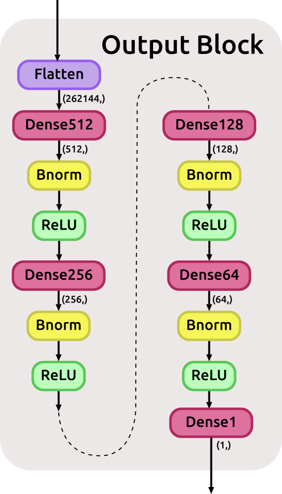
Figure 3: Diagram of the output block: a bottleneck-structured sequence — Dense/Batch Normalization /ReLU gradually decreasing feature hyperspace ($512$, $256$, $128$, $64$ and finally $1$).

2.2 Error Analysis

Uncertainty estimates are critical for assessing confidence in scientific measurements. Nevertheless, cogent and interpretable methods for uncertainty estimation in deep learning remain elusive. There are several types of uncertainty that are useful in assessing scientific confidence. They may be broadly classified into two categories — aleatoric (statistical) and epistemic (systematic). Aleatoric uncertainties encompass effects that are unknown and change with the acquisition of each piece of data. These uncertainties are expected to decrease, for a given fixed model, with an increase in sample-taking in the predictions process. For strong lenses, this would include shot noise in CCD imaging. Epistemic uncertainties, on the other hand, include errors due to things that can be known but are neglect in the current investigation, for instance, certain effects that are not modelled. For a given model these do not decrease with an increase in sample-taking. However, in the case of Deep Learning Regression which is a data driven model, if one feeds the network with more data during the training process that would change the model and, in principle could lower our ignorance about which model generated the collected training data (Kendall and Gal, 2017). We named the total error, which includes the epistemic and aleatoric, predictive error. Standard error propagation is currently untenable, because there are not measurements of errors in raw images without performing some modeling in the first place. Additionally, there is no way to propagate that uncertainty, if it existed, through a deep learning model to the inferred parameters: we would need to know the uncertainties on the model parameters, but this error is not well known. Ideally, we would be able to perform uncertainty estimates of all parameters in a fully Bayesian framework. Bayesian neural networks may provide Gaussian process approximations of the variance in the output parameters (Lee et al., 2017); however, parameters may not all have Gaussian errors.

Another method that has been used recently is Concrete Dropout, which was first described by Gal and Ghahramani (2016); Gal et al. (2017), and first used in strong lens modeling by Levasseur et al. (2017). In this method, to estimate uncertainties on the parameters of interest, we compute the PDF of the predictions using the concrete dropout technique. Concrete dropout approximates a posterior distribution $p\left(Y|X\right)$ of the predicted physical parameter $Y$, given an input image $x$ in a Bayesian framework. We interpret our model in the variational perspective (Jordan et al., 1999; Graves, 2011). We consider that dropping out neural network weights,i .e., performing dropouts, as a sampling from the distribution $p(\omega|{\bf X},{\bf Y})$ of the weights $\omega$, which are learned via a set of inputs ${\bf X}=\{x_{1},...,x_{N}\}$ and the corresponding output parameters ${\bf Y}=\{y_{1},...,y_{N}\}$ (Gal and Ghahramani, 2016).

2.2.1 epistemic (model) uncertainty

Considering that neural networks can theoretically provide universal approximations, using dropout in this way is analogous to sampling over the space of functions (Gal and Ghahramani, 2016; Gal, 2016). The error associated with this sampling is related to the ignorance of the model; this is known as epistemic uncertainty. Basics of method: a sampling a trained deep learning model could be interpreted in a Bayesian framework by optimizing its dropout rates and sampling the posterior $p(y|x,{\bf X},{\bf Y})$ with the forward passes. Then, once the network is trained, the sampling of predicted values are simply forward passes upon which we apply dropouts, and thus calculate a posterior for the predictions. This technique is known as Monte Carlo dropout (Gal and Ghahramani, 2016).

However, defining the dropout rate is not a trivial task. For example, a fixed dropout probability will penalize larger weights when compared to the smaller ones (Gal et al., 2017), since when larger weights are dropped, they are likely to have a bigger impact in the results. To minimize the epistemic error in this scenario, one should optimize to lower-magnitude weights. For instance, the $0$-epistemic uncertainty would correspond to a situation in which we have all weights set to $0$, since the predictions would always be 0, however, the model would not perform any prediction at all. Therefore, the aim of defining a dropout rate is not to get optimized precision, but to find a point where epistemic errors can be reasonably defined. Some authors proposed a grid-search for this task. However, this procedure may be prohibitive in big and complex architectures.

In the variational scheme, one may define a procedure to optimize the dropout rate. The problem can be stated as follows: for a network, we can compute the PDF of a predicted value $y$ with input $x$ as:

$$p(y|x,{\bf X},{\bf Y})=\int p(y|x,\omega)\,p(\omega|{\bf X},{\bf Y})\,\,d\omega\,.$$ (1)

The posterior $p(\omega|{\bf X},{\bf Y})$ has explicit dependence on the training dataset, and its form is generally infeasible to derive. Thus we define an analytical variational distribution, $q_{\theta}(\omega)$, with parameters $\theta$ such that

$$p(y|x)\approx\int p(y|x,\omega)\,q_{\theta}(\omega)\,\,d\omega\,.$$ (2)

We use a classification task as an example. From there, we develop a strategy for regression. For simplicity, in a classification task, it can be shown that one can derive the parameters from $q_{\theta}(\omega)$ by maximizing the log-evidence lower bound (Fox and Roberts, 2012):

$$L=\int q_{\theta}(\omega)\,\log p({\bf Y}|{\bf X},\omega)\,\,d\omega-\mathrm{KL}(q_{\theta}(\omega)||p(\omega))\,.$$ (3)

The first term corresponds to a traditional loss term in classification tasks — i.e., a log-likelihood of the outputs for the training set — which can be replaced with a Gaussian loss in regression tasks. The integral can be performed by a Monte Carlo integration procedure. The second term is $\mathrm{KL}$ divergence, which parametrizes the distance between the distributions $p(\omega)$ and $q_{\theta}(\omega)$, thus minimizing it during the training process. The $\mathrm{KL}$ divergence term can be approximated by a $L_{2}$ regularization (Gal and Ghahramani, 2016). For a set of parameters $\theta=\{{\bf M},p_{l}\}_{l=1}^{L}$ in which ${\bf M}_{l}$ are the mean weight matrices and $p$ are the $l^{\rm th}$ layer, a typical choice for $q_{\theta}(\omega)$ is to define:

$$\begin{split}q_{\theta}(\omega)&=\prod_{l}q_{{\bf M}_{l}}({\bf W}_{l}),\\ q_{{\bf M}_{l}}({\bf W}_{l})&={{\bf M}_{l}}\cdot\mathrm{diag}[\text{Bernoulli}(1-p_{l})^{K_{l}}],\end{split}$$ (4)

where the set of random weight matrices are $\omega=\{{\bf W}_{l=1}^{L}\}$, with $L$ layers and dimensions of each weight matrix are $K_{l}$ and $K_{l+1}$. The Bernoulli variables, $z=\text{Bernoulli}(1-p_{l})$, drop some neural network weights with its given probability.

Thus, a deep learning model could be interpreted in a Bayesian framework by optimizing its dropout rates and sampling the posterior $p(y|x,{\bf X},{\bf Y})$ with the forward passes. However, in some cases, there may be some issues in performing this optimization. It can be shown that finding the minimum of the $\mathrm{KL}$ divergence term in Eqn. 3 is equivalent to maximizing the entropy of a Bernoulli random variable with probability $1-p$. This penalizes larger models trained on small amounts of data, because it pushes the dropout rate close to $p=0.5$ in comparison to smaller models (Gal et al., 2017). Therefore, smaller models would have lower optimized dropout rates in the low-data regime. Nevertheless, with epistemic uncertainty, the dropout rate is lowered for both large and small model as we feed the neural network with more data.

There remain caveats when evaluating the derivative of the objective function with respect to a dropout rate in discrete Bernoulli distributions. Therefore, we follow the prescription from Gal et al. (2017) and replace the Bernoulli variables for Concrete distribution (Maddison et al., 2016) — i.e., a continuous distribution with the ability to approximate discrete random variables. We sampled from the concrete distribution that approximates the one-dimensional Bernoulli, equivalent to a binary random variable:

$$\tilde{z} =\text{sigmoid}\left(\frac{1}{t}\cdot\left(\log p-\log(1-p)+\log u-\log(1-u)\right)\right),$$ (5)

where $t$ is a temperature parameter and $u$ is the uniform distribution $u\sim\mathcal{U}(0,1)$.

After training, we derive $10^{3}$ realizations for each system. We define the $68\%$, $95\%$, and $99\%$ confidence intervals. We compared the confidence interval of the scatter of the medians — scatter from different objects with same truth value — with confidence levels from the individual object parameter realizations. The confidence intervals from the Concrete Dropout realizations were little wider but followed the scatter confidence intervals closely.

2.2.2 Aleatoric (statistical) uncertainties

In principle, if one compares the results considering only epistemic error disregarding aleatoric errors to the truth values it might get unrealistic results. To address the aleatoric errors to the total (predictive) error one must take into account what are the noise proprieties of the dataset. For a homeostatic data set — in which all the data has similar noise proprieties — this is usually done by adding a random uncertainty that can be manually fine-tuned. As the data presents diferent levels of signal-to-noise ratio we estimated the aleatoric uncertainties in a heteroscedastic framework: we train the neural networks to predict the $\sigma_{k}$, the observation noise parameter for the $k$ output parameter. This is done by optimizing $\sigma_{k}$ in the regression loss term, $L_{R}$ which corresponds to the first term of equation 3 for regression tasks and it is given by:

$$L_{R}=\sum_{k}\frac{-1}{2\sigma_{k}^{2}}||{y}_{n,k}-\hat{{y}}_{n,k}({\bf x}_{n},\omega)||^{2}-\frac{1}{2}\log{\bf\sigma}_{k}^{2},$$ (6)

where $y_{n,k}$ and $\hat{{y}}_{n,k}$ are the true values and the predict values, respectively, for the $n$ training sampling. Thus, there is no need of labelled aleatoric uncertainties.

2.2.3 Systematic uncertainties

However, this still may not encapsulate all systematic uncertainties, which would be revealed in noise-free input data. Additionally, besides the source of epistemic (model) errors from the deep model uncertainty itself that might remain other degeneracies that can bias or scatter the results. For instance, in wide-field survey imaging, the pixel size and PSF are typically larger than in space-based observations. There may also be degeneracies that can be more complex than random scatter on the predicted value. The Strong lensing Systems may have multiple source images that can be distorted in several ways, and can also be blended with the lens galaxy. Additionally, the lensed image has a parameter space with of order ten independent variables. This might be a relevant origin of systematic errors when trying to extract information from images. For example, it can be significantly easier to infer the Einstein radius, $\theta_{E}$, of a strong lensing system in cases where the light from the lensed source is not blended with the light from the lens galaxy than in cases where it is, even if the noise level in the images are the same.

In order to evaluate a possible bias or scatter in our results, we visually compared the median predictions in our training sample to the respective truth values. We observed that, even when considering the epistemic uncertainties, there was a small bias in some of our model predictions that scaled linearly. To address this problem, we adopted the following procedure: we performed a linear fit between model predictions and the truth values, and then subtracted the bias in the predictions. We then used the same linear fit to remove bias in the test data set. Therefore, our model comprises of a deep learning prediction and a linear scale correction. After the fitting procedure, we found that the percentile error in the scatter in the medians and the percentile error due to the sampling performed by dropouts were consistently symmetric around the median and in most of the range around the $y=x$ line, except for certain high and low boundaries that corresponded to regions where the model has fewer samples. We discuss this further in section 6.

3 Simulated Data

To optimally train, validate and test a neural network for strong lensing analysis, we require a large image catalog of strong lenses. Given the paucity of known strong lenses in the current census ($\sim$1000 lenses to date), we used simulated lenses from LensPop (Collett, 2015a) to define different sets of images for training, validation and testing purposes. Here, we present a brief overview of the procedure used in the LensPop algorithm. For a complete description of LensPop, we refer interested readers to Collett (2015b).

LensPop first generates a synthetic population of galaxy-scale strong lensing systems in the sky. For the lens population, LensPop assumes Singular Isothermal Ellipsoid (SIE) profiles for all lenses, with masses drawn from the velocity dispersion function of SDSS galaxies (Choi et al., 2007). Observations show that elliptical galaxies, which dominate the lensing probability of the universe (see, e.g., Oguri and Marshall, 2010, and references within) , are well-approximated by SIE mass profiles (Auger et al., 2010; Koopmans et al., 2006b). The redshift of the lenses are drawn independently from the mass from the differential comoving volume function. The light profile of the lens is assumed to follow a de Vaucouleurs profile (de Vaucouleurs, 1948) that is aligned and concentric with the mass. The lens colors are assumed to follow the rest-frame SED of a galaxy whose star formation occurred 10 Gyrs ago. For the source population in LensPop, the source light have elliptical exponential light profiles, with magnitude, color and redshift distributions drawn from the sky catalogs of A. J. Connolly (2010).

The observing conditions of the imaging survey are then simulated and applied to the synthetic lenses to produce a mock catalog of lens imaging data that mimics that survey. In this work, we simulated the observing and instrumental capabilities of the DES survey to produce lenses with DES-like image quality. The mock images are created by first pixelating the model lens image to the pixel scale of the detector of the survey instrument. The pixelated images are then convolved with circular atmospheric PSFs. Poisson noise from the lens, source, uniform sky background and CCD read noise are then added to the mock images. The zero-points, exposure-times, number of exposures, pixel-scale, read noise, filter bands and survey area are taken from DES survey specifications. The seeing and sky brightness are stochastic variables drawn from DES data and are described in Table 1 of Collett (2015b).

Every simulated lens in our data set is deemed DES-observable. We follow the criteria set in Collett (2015b) to determine which lensing systems are detectable by DES. All detectable lenses must be multiply imaged. Therefore we have:

$$\theta_{\rm E}^{2}>x_{s}^{2}+y_{s}^{2},$$ (7)

where $\theta_{\rm E}$ is the Einstein radius, and $x_{s}$ and $y_{s}$ are the unlensed source position relative to the lensing galaxy. In at least one of the $g,r,i$ bands, the image and counter-image must be resolved. Hence, we also require that:

$$\theta_{\rm E}^{2}>r_{s}^{2}+(s/2)^{2},$$ (8)

where $r_{s}^{2}$ is the half-light radius of the source, and $s$ is the seeing. Additionally, the tangential shear of the magnified source images in the image plane must also be resolved, and the magnification has to be large enough that the source images are noticeably sheared. Following Collett (2015b), we adopt:

$$\mu_{\mathrm{total}}r_{s}>s\quad\mathrm{and}\quad\mu_{\mathrm{total}}>3,$$ (9)

where $\mu_{\mathrm{total}}$ is the total magnification of the source. Finally, the signal-to-noise ratio, $S/N_{\mathrm{total}}$ must be high enough that it is feasible to identify the lens and to determine if the above criteria is met. Also following Collett (2015b), we set

$$S/N>20.$$ (10)

Using LensPop, we generated $18,600$ simulated DES-observable galaxy-galaxy lensing systems. The distributions of the Einstein radii ($\theta_{\rm E}$), velocity dispersion ($\sigma_{\mathrm{v}}$), and lens and source redshifts ($z_{L}$, $z_{S}$) in the DES simulated dataset agrees with that of Collett (2015b). Fig. 4 shows a representative random sample of 20 DES-observable systems from the total dataset.

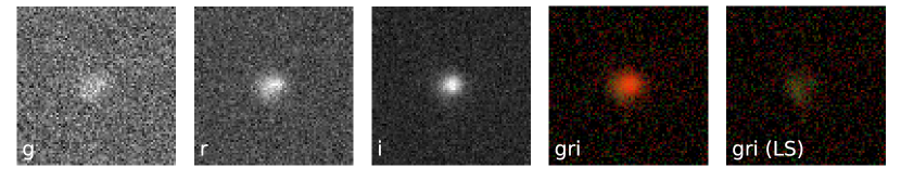
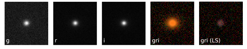
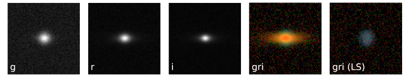
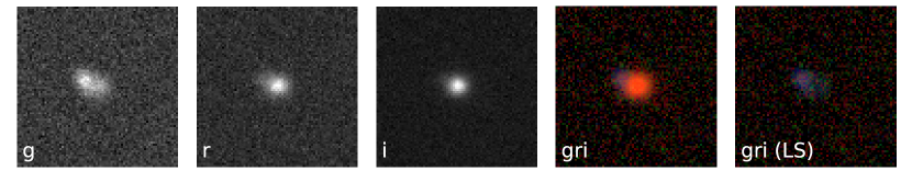
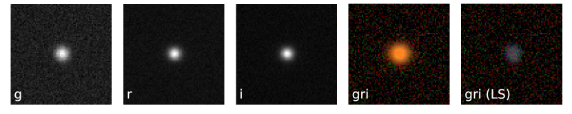
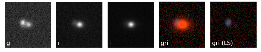
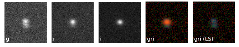
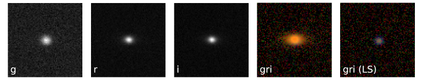
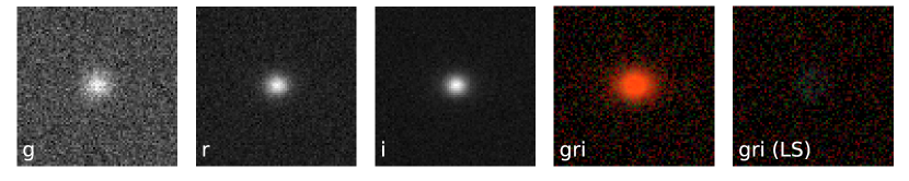
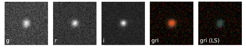
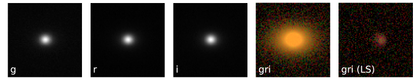
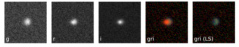
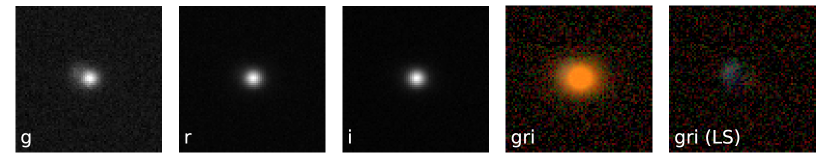
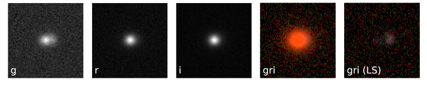
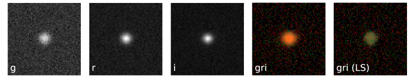
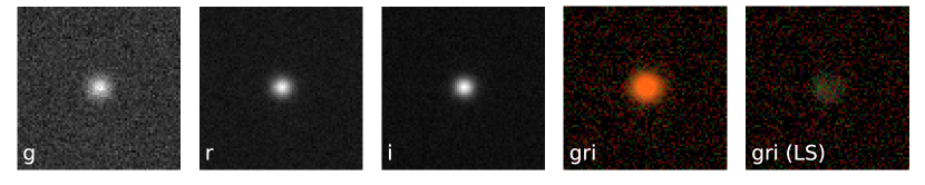
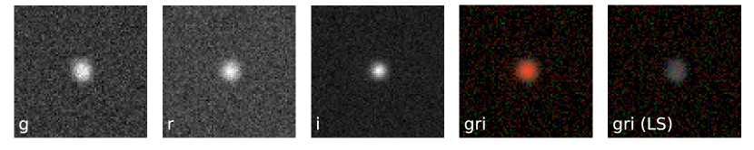
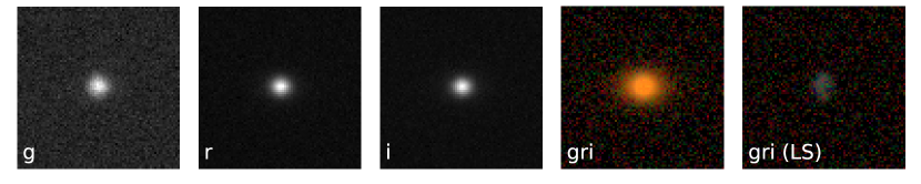
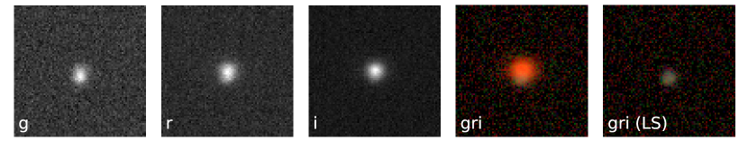
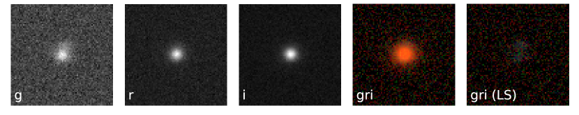
Figure 4: A random selection of 20 DES-observable lens systems from the $\mathrm{LensPop}$ simulation. For each system, the individual $g$, $r$, $i$, band images, as well as false-color $gri$ composite image with lens galaxy (’gri’) and without lens galaxy (’gri (LS)’), are shown from left to right. False-color images were made following Lupton et al. (2004). Images are sorted left-to-right, top-to-bottom by increasing Einstein radii. Refer to §LABEL:sec:simulations for further information on the simulated images dataset.

4 Training the Inception Deep Learning Model

The strong lensing sample was divided into two groups: $80\%$ for training and validation purposes, and $20\%$ for testing. The training subset is the only one used to update the weights of the network in the backpropagation algorithm (Ruder, 2016). We trained the Inception architecture for the parameters $\theta_{\rm E}$, $\sigma_{\rm v}$, $z_{\rm l}$ and $z_{\rm s}$ both together, all predictions at once and individually (in which the output core diagram presented in Fig. 2 should be considered with only one branch). The fine-tuned hyperparameters used for training the architecture were found by manually changing their values within a certain range until the (local) maximum accuracy on regression was achieved. The chosen batch size for training was $2,000$, while the maximum number of epochs was set to $400$. To avoid overfitting, and to improve model convergence, both a learning rate reducer and an early stopper were used. The training was performed with an Adam optimizer. The model was trained on a 24-core Intel Xeon CPU X5670 ($2.93$ GHz) and a GeForce GTX 1080 GPU.

The training time of each model was $\sim 4$ hours. In Fig. 5, we present the training diagnostic loss vs. epoch for the $z_{s}$, where we set a fixed number of epochs to $200$ for the training and validation dataset. The plot indicates the optimization performance on each sample, training and validation, and suggests no strong overfitting. Both $\sigma_{\rm v}$, $\theta_{\rm E}$, $z_{L}$ and also the network that outputs all four parameter at once presented similar curves.

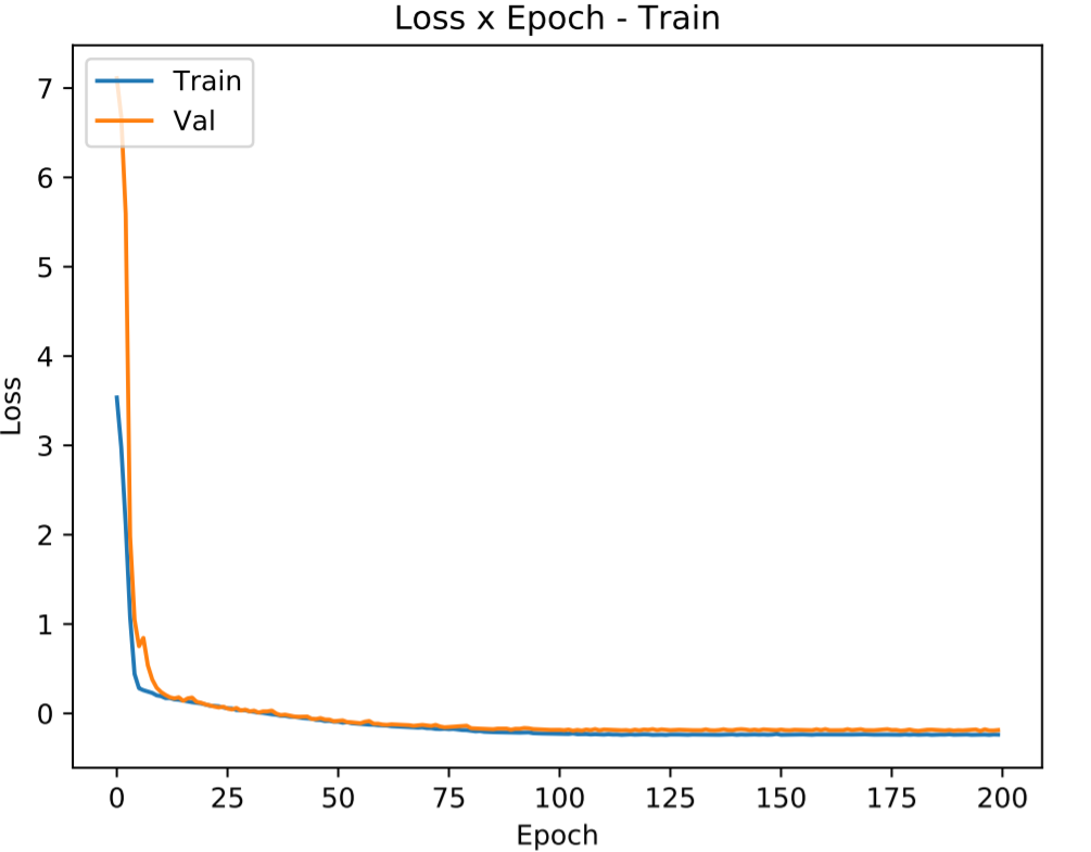
Figure 5: Loss versus epoch on training phase for $z_{s}$.

5 Results

The regression was performed with the trained models on our test sample consisting of $3720$ systems. The testing sample takes less than $\sim 1$ sec to infer $10^{3}$ realizations on each strong lens system. We present the predicted results for $\theta_{\rm E}$, $\sigma_{\rm v}$, $z_{\rm l}$ and $z_{\rm s}$ residuals relative to truth, along with the distributions of each value in Fig. 6 in the network that predicts all four parameters at once. We observed that, for most of the ranges, the predicted values remained within $\pm 10\%-15\%$ of the truth values, except for the $z_{\rm s}$. We noticed higher deviations from truth at low and high values, which correspond to smaller sample sizes in our training dataset. In those regions, some bias remains in the predicted medians and truth values, though they are consistent at $68\%$ confidence level. In the top portion of Fig. 7, we present the median of the fractional deviation and the $68\%$ confidence level percentile for both predicting one parameter at a time (red) and all parameters at once (blue). We do not notice any strong bias in any parameter. In the bottom portion the same figure, we evaluate the size of the high-deviation sample, defined as fractional deviation higher than $15\%$). The results in both cases, red and blue, were similar, although it suggests that predicting several parameters at a time may lower the sample of high-deviation lenses at least for $z_{L}$. For all parameters, except $z_{\rm s}$, the average fractional deviations in the whole testing sample was lower than $10\%$.

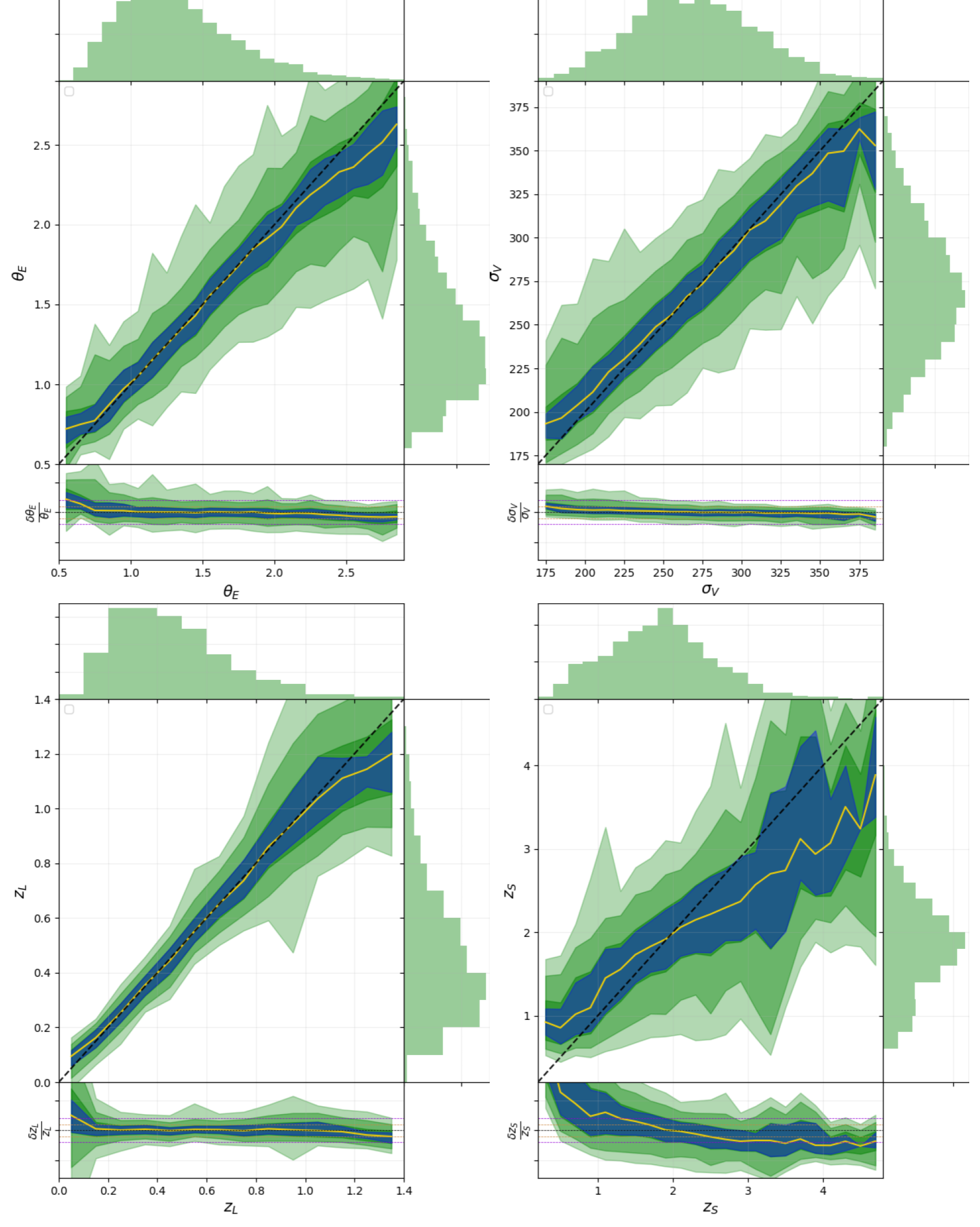
Figure 6: True values vs predicted values and the residuals for: the Einstein Radius,$\theta_{\rm E}$ (top-left), velocity dispersion, $\sigma_{V}$ (top-right), lens redshift, $z_{L}$ (bottom-left) and source redshift, $z_{S}$ (bottom-right). The green shadows are the percentile corresponding to $1-2-3$ sigma area, the blue shadows are the 1-sigma scatter of medians predicted values.

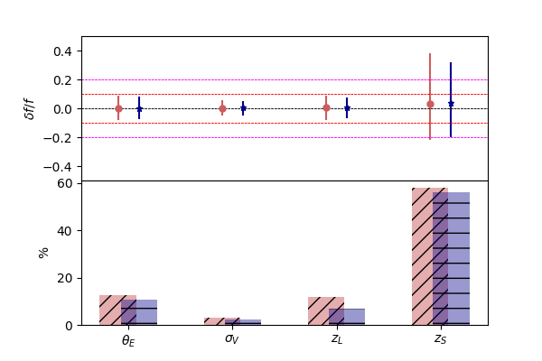
Figure 7: The fractional deviation on the full testing sample using models that predicts a single parameter (red circles) and the model that predicts all $4$ parameters at once (Blue star), where the dashed lines represent the $0.0$ (black),$0.1$ (red),$0.2$ (magenta) deviations (top). The percentage of objects with more than $0.15$ fractional deviation (bottom).

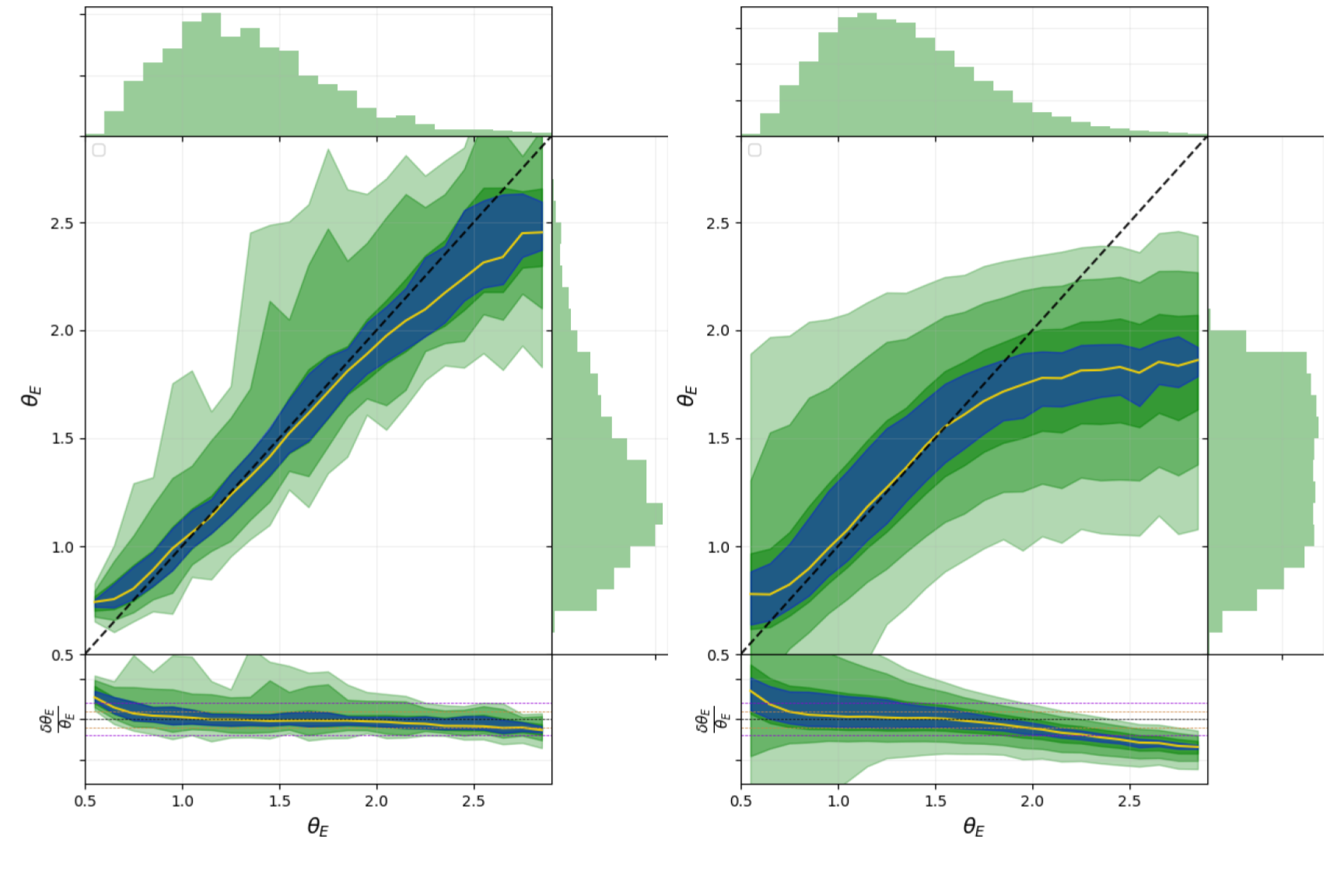
Figure 8: True vs predicted values of $\theta_{\rm E}$ and the residuals for a $90\%/10\%$ (left) $10\%/90\%$ training/test split. The green shadows are the percentile corresponding to $1-2-3$ sigma area, the blue shadows are the 1-sigma scatter of medians predicted values.

We also investigated how the fractional deviation changes as function of other physical values, like magnitude, signal to noise ratio and size of the lensing object. In most cases, we found regions of higher bias or error corresponding to low parameter sampling, suggesting that the uncertainty or bias could be overcomed with more data. However, there are some interesting cases, such as the ones presented in Fig. 9. In these figures we observed that smaller/bigger $\theta_{\rm E}$ might be correlated to fractional deviations up to $\approx+80\%$/$-40\%$ considering the $68\%$ error bars for $\theta_{\rm E}>0.7$ arcsec in the network that outputs all parameters at once. Though the error bars are wide and it includes the $0\%$ deviation, it is worth mentioning that there are regions in the high $\theta_{\rm E}$ end that have a lower number of examples and the errors might be poorly defined in those regions. The $\theta_{\rm E}$ is connected to $z_{\rm s}$ though the cosmological distances. In the $z_{\rm l}$ case we observe that lower/higher velocity dispersion may be linked to $\approx+20\%$/$-10\%$ deviations in the medians. Additionally to the presented plots, we also observed that $\theta_{\rm E}$ predicted errors are wider by a factor $\sim 2$, i.e., $\sim\pm 20\%$ for $\sigma_{\rm v}$ below $230$ km/s. As $\sigma_{\rm v}$ scales with the mass and therefore are connected to $\theta_{\rm E}$ these suggests that as the lensing effect gets weaker the uncertainty raises.These results might be useful if one is trying to define a more accurate sample or trying to fine tune the models. The results did not changed significantly in terms of accuracy as function of signal to noise ratio, this is probably due to the selection criteria $S/N>20$ in the simulations which requires that the strong lensing should be easy detected. Lastly, we evaluated the effect of trainind/test dataset split. In the Fig. 8 two different train/test sets with $90\%/10\%$(left) and $10\%/90\%$ (right) are shown. The right figure presents wider errorbars, e.g., for $\theta_{\rm E}<1.0^{\prime\prime}$ the high limit of $3$ sigma uncertainty is $2.0^{\prime\prime}$. It is worth noticing that the methods became flat, considering the medians for $\theta_{\rm E}\gtrapprox 2.0^{\prime\prime}$. These results support the importance of using as much data as possible in data driven models such as the one presented in order to make reasonable predictions.

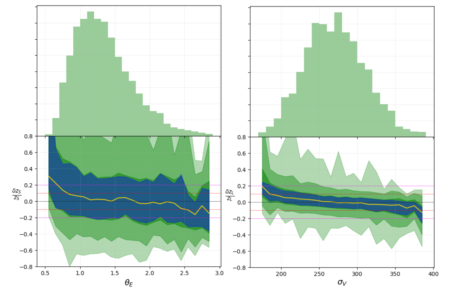
Figure 9: The fractional deviation from true values in source redshift $z_{\rm s}$ from as function of Einstein Radius $\theta_{E}$ (left) and lens redshift $z_{\rm l}$ as function of velocity dispersion $\sigma_{\rm v}$ (right). The green shadows are the percentile corresponding to $1-2-3$ sigma area and the blue shadows are the 1 sigma scatter of medians predicted values. The dashed lines represent the $0.0$ (black),$0.1$ (red),$0.2$ (magenta) deviations.

6 Discussion and concluding remarks

We presented the prediction of astrophysical features of strong lensing sytems in simulated wide-survey images using a deep neural net model. These parameter predictions include estimates of both epistemic and aleatoric uncertainties, and we verified that the scatter on thousands of individual systems predictions were lower than this uncertainty. In particular, the velocity dispersion was constrained to lower than $10\%$ level using only $3$ bands. The current results support that we could use deep learning as a tool for quick catalog generation and a reliable analysis that could outperform more conventional methods (e.g., MCMC) in computation time and without highly specialized experts. This, in principle could be used to select systems for further investigation or be used in statistical analysis that requires this $\sim 15\%$ level performance, for instance in galaxy-galaxy strong lensing cosmology (Cao et al., 2015; Chen et al., 2018), where we could use the $\theta_{\rm E}$ combined with an independent measurement of $\sigma_{\rm v}$ to derive distance ratios or deriving galaxy mass-density profiles (Li et al., 2018a).

At low and high values of each parameter, we observed a bias and we observed an expected high uncertainty. This likely caused by the relatively low number of training examples in these regions. Additionally, systems with smaller Einstein radii are likely harder to estimate due to the lack of differentiation of canonical lensing features in those systems. More examples in these regions of parameter space could lower the uncertainty. However, as the model confidence level improves systematic errors associated with this parameter region may also be revealed. In future work, we seek to a) address the interplay and trade-offs for various kinds of uncertainties; and b) to explore how changes in image quality affect these results.

The estimations from velocity dispersion deviations were in a regime lower than $10\%$. This precision is competitive with spectroscopic surveys such as BELLS (Bolton et al., 2012), and SLACS (Bolton et al., 2006). It is worth noticing that the input of our method includes not only the information from three bands, but also morphology, and strong lensed sources which are expected to be useful to constrain the velocity dispersion. In fact, if the $\theta_{\rm E}$ or angular separation $\theta$, $z_{l}$ and $z_{s}$ are well-constrained, one could estimate the velocity dispersion $\sigma_{v}$ with this level of accuracy, given a density profile and a cosmology (Davis et al., 2003). In fact, if the velocity dispersion is constrained from strong lensing, it could be applied to modified gravity tests such as Cao et al. (2017); Schwab et al. (2009). This can be further investigated with techniques, such as the Local Interpretable Model-Agnostic Explanations (LIME; Ribeiro et al., 2016). This will also be the subject of future investigation.

It should be noted that due to the somewhat idealized nature of $\mathrm{LensPop}$’s prescription for simulating a DES-like image dataset, the uncertainties quantified here may be lower than the uncertainty in our inferences from real imaging data. While $\mathrm{LensPop}$’s prescription is well-motivated by both theoretical and empirical considerations, it makes a number of simplifying assumptions about the populations of lenses and sources, as well as the simulated observing conditions of the systems (some of which are discussed in §7 of Collett (2015b)). Real strong lensing systems are likely to have characteristics that deviate from these assumptions to various extents.

More crucially, $\mathrm{LensPop}$ assumes each lensing system is found in isolation. In reality, elliptical galaxies, which constitutes the majority of galaxy-scale lenses, tend to cluster, which leads to external perturbations to the lensing potential of the lens system due to nearby masses, as well as the crowding of the field-of-view near the lens system by these objects. $\mathrm{LensPop}$ also ignores objects that may be situated along the line-of-sight of the lens by coincidence. These inhomogeneous scenarios can result in higher uncertanties when the regression is applied to real data.

In such regimes, one needs to properly address the systematic uncertainties from the data. A possible way to reduce the impact of uncertainties in data due to factors unaccounted for in the idealized simulations might be to do transfer learning or domain adaption, in order words, start from the models presented in this paper, or parts of it, and make a fine tuning, for real data. However, since there are orders of magnitude fewer strong lensing systems discovered in real data to date, to properly train this scheme is a major challenge and one might also need to make use of data augmentation methods. We are currently evaluating the relevance of idealized simulations by working on simulations with increased degrees of realism. This work therefore represents a novel step towards building a more robust framework to analyse strong lensing systems found in current and future ground-based survey data.

It is worth mentioning a significant part of the real data might have inhomogeneous observational conditions and a the fine tuning should consider simulations with different exposure times/noise levels in different bands, or focus on real lenses with higher signal-to-noise ratios.

References

- A. J. Connolly (2010) A. J. Connolly, John Peterson, J.G.J.R.A.J.B.C.C.C.F.C.R.G.D.K.G.E.G.R.L.J.Z.I.J.J.M.J.S.M.K.V.L.K.S.K.S.L.J.P.A.R.N.T.J.A.T.M.Y., 2010. Simulating the lsst system. URL: https://doi.org/10.1117/12.857819, doi:10.1117/12.857819.
- Abdel-Hamid et al. (2014) Abdel-Hamid, O., Mohamed, A.r., Jiang, H., et al., 2014. Convolutional neural networks for speech recognition. IEEE/ACM Transactions on audio, speech, and language processing 22, 1533–1545.
- Abdelsalam et al. (1998) Abdelsalam, H.M., Saha, P., Williams, L.L.R., 1998. Non-parametric reconstruction of cluster mass distribution from strong lensing - Modelling Abell 370. Mon. Not. Roy. Astron. Soc. 294, 734. doi:10.1046/j.1365-8711.1998.01356.x, arXiv:astro-ph/9707207.
- Auger et al. (2010) Auger, M.W., Treu, T., Bolton, A.S., et al., 2010. The Sloan Lens ACS Survey. X. Stellar, Dynamical, and Total Mass Correlations of Massive Early-type Galaxies. Astrophys. J. 724, 511--525. doi:10.1088/0004-637X/724/1/511, arXiv:1007.2880.
- Bartelmann et al. (1998) Bartelmann, M., Huss, A., Colberg, J.M., Jenkins, A., Pearce, F.R., 1998. Arc statistics with realistic cluster potentials. IV. Clusters in different cosmologies. Astr. & Astroph. 330, 1--9. arXiv:astro-ph/9707167.
- Bayer et al. (2018) Bayer, D., Chatterjee, S., Koopmans, L., et al., 2018. Observational constraints on the sub-galactic matter-power spectrum from galaxy-galaxy strong gravitational lensing. arXiv preprint arXiv:1803.05952 .
- Bayliss (2012) Bayliss, M.B., 2012. Broadband Photometry of 105 Giant Arcs: Redshift Constraints and Implications for Giant Arc Statistics. Astrophys. J. 744, 156. doi:10.1088/0004-637X/744/2/156, arXiv:1108.1175.
- Belagiannis et al. (2015) Belagiannis, V., Rupprecht, C., Carneiro, G., Navab, N., 2015. Robust optimization for deep regression, in: Proceedings of the IEEE International Conference on Computer Vision, pp. 2830--2838.
- Belokurov et al. (2009) Belokurov, V., Evans, N.W., Hewett, P.C., et al., 2009. Two new large-separation gravitational lenses from SDSS. Mon. Not. Roy. Astron. Soc. 392, 104--112. doi:10.1111/j.1365-2966.2008.14075.x, arXiv:0806.4188.
- Bolton et al. (2012) Bolton, A.S., Brownstein, J.R., Kochanek, C.S., et al., 2012. The boss emission-line lens survey. ii. investigating mass-density profile evolution in the slacs+ bells strong gravitational lens sample. The Astrophysical Journal 757, 82.
- Bolton et al. (2006) Bolton, A.S., Burles, S., Koopmans, L.V., Treu, T., Moustakas, L.A., 2006. The sloan lens acs survey. i. a large spectroscopically selected sample of massive early-type lens galaxies. The Astrophysical Journal 638, 703.
- Bom et al. (2017) Bom, C.R., Makler, M., Albuquerque, M.P., Brandt, C.H., 2017. A neural network gravitational arc finder based on the Mediatrix filamentation method. Astr. & Astroph. 597, A135. doi:10.1051/0004-6361/201629159, arXiv:1607.04644.
- Bradač et al. (2009) Bradač, M., Treu, T., Applegate, D., et al., 2009. Focusing Cosmic Telescopes: Exploring Redshift z ~ 5-6 Galaxies with the Bullet Cluster 1E0657 - 56. Astrophys. J. 706, 1201--1212. doi:10.1088/0004-637X/706/2/1201, arXiv:0910.2708.
- Cabanac et al. (2007) Cabanac, R.A., Alard, C., Dantel-Fort, M., et al., 2007. The CFHTLS strong lensing legacy survey. I. Survey overview and T0002 release sample. Astr. & Astroph. 461, 813--821. doi:10.1051/0004-6361:20065810, arXiv:arXiv:astro-ph/0610362.
- Caminha et al. (2016) Caminha, G.B., Grillo, C., Rosati, P., et al., 2016. CLASH-VLT: A highly precise strong lensing model of the galaxy cluster RXC J2248.7-4431 (Abell S1063) and prospects for cosmography. Astr. & Astroph. 587, A80. doi:10.1051/0004-6361/201527670, arXiv:1512.04555.
- Caminha et al. (2015) Caminha, G.B., Karman, W., Rosati, P., et al., 2015. Discovery of a faint star-forming multiply lensed Lyman-alpha blob. arXiv:1512.05655 arXiv:1512.05655.
- Cao et al. (2015) Cao, S., Biesiada, M., Gavazzi, R., Piórkowska, A., Zhu, Z.H., 2015. Cosmology with strong-lensing systems. The Astrophysical Journal 806, 185. URL: http://stacks.iop.org/0004-637X/806/i=2/a=185.
- Cao et al. (2017) Cao, S., Li, X., Biesiada, M., et al., 2017. Test of parametrized post-newtonian gravity with galaxy-scale strong lensing systems. The Astrophysical Journal 835, 92.
- Carrasco et al. (2010) Carrasco, E.R., Gomez, P.L., Verdugo, T., et al., 2010. Strong Gravitational Lensing by the Super-massive cD Galaxy in Abell 3827. Astrophys. J. Lett. 715, L160--L164. doi:10.1088/2041-8205/715/2/L160, arXiv:1004.5410.
- Chen et al. (2018) Chen, Y., Li, R., Shu, Y., 2018. Assessing the effect of lens mass model in cosmological application with updated galaxy-scale strong gravitational lensing sample. arXiv preprint arXiv:1809.09845 .
- Choi et al. (2017) Choi, K., Fazekas, G., Sandler, M., Cho, K., 2017. Convolutional recurrent neural networks for music classification, in: 2017 IEEE International Conference on Acoustics, Speech and Signal Processing (ICASSP), IEEE. pp. 2392--2396.
- Choi et al. (2007) Choi, Y.Y., Park, C., Vogeley, M.S., 2007. Internal and Collective Properties of Galaxies in the Sloan Digital Sky Survey. Astrophys. J. 658, 884--897. doi:10.1086/511060, arXiv:astro-ph/0611607.
- Coe et al. (2010) Coe, D., Benítez, N., Broadhurst, T., Moustakas, L.A., 2010. A High-resolution Mass Map of Galaxy Cluster Substructure: LensPerfect Analysis of A1689. Astrophys. J. 723, 1678--1702. doi:10.1088/0004-637X/723/2/1678, arXiv:1005.0398.
- Coe et al. (2008) Coe, D., Fuselier, E., Benítez, N., et al., 2008. LensPerfect: Gravitational Lens Mass Map Reconstructions Yielding Exact Reproduction of All Multiple Images. Astrophys. J. 681, 814--830. doi:10.1086/588250, arXiv:0803.1199.
- Collett (2015a) Collett, T.E., 2015a. The Population of Galaxy-Galaxy Strong Lenses in Forthcoming Optical Imaging Surveys. Astrophys. J. 811, 20. doi:10.1088/0004-637X/811/1/20, arXiv:1507.02657.
- Collett (2015b) Collett, T.E., 2015b. The Population of Galaxy-Galaxy Strong Lenses in Forthcoming Optical Imaging Surveys. Astrophys. J. 811, 20. doi:10.1088/0004-637X/811/1/20, arXiv:1507.02657.
- Cooray (1999) Cooray, A.R., 1999. Cosmology with galaxy clusters. III. Gravitationally lensed arc statistics as a cosmological probe. Astr. & Astroph. 341, 653--661. arXiv:astro-ph/9807147.
- Csáji (2001) Csáji, B.C., 2001. Approximation with artificial neural networks. Faculty of Sciences, Etvs Lornd University, Hungary 24, 48.
- Davis et al. (2003) Davis, A.N., Huterer, D., Krauss, L.M., 2003. Strong lensing constraints on the velocity dispersion and density profile of elliptical galaxies. Monthly Notices of the Royal Astronomical Society 344, 1029--1040.
- de Vaucouleurs (1948) de Vaucouleurs, G., 1948. Recherches sur les Nebuleuses Extragalactiques. Annales d’Astrophysique 11, 247.
- Despali et al. (2018) Despali, G., Vegetti, S., White, S.D.M., Giocoli, C., van den Bosch, F.C., 2018. Modelling the line-of-sight contribution in substructure lensing. Mon. Not. Roy. Astron. Soc. 475, 5424--5442. doi:10.1093/mnras/sty159, arXiv:1710.05029.
- Diego et al. (2005) Diego, J.M., Protopapas, P., Sandvik, H.B., Tegmark, M., 2005. Non-parametric inversion of strong lensing systems. Mon. Not. Roy. Astron. Soc. 360, 477--491. doi:10.1111/j.1365-2966.2005.09021.x, arXiv:astro-ph/0408418.
- Dye et al. (2018) Dye, S., Furlanetto, C., Dunne, L., et al., 2018. Modelling high-resolution alma observations of strongly lensed highly star-forming galaxies detected by herschel. Monthly Notices of the Royal Astronomical Society 476, 4383--4394.
- Eales et al. (2010) Eales, S., Dunne, L., Clements, D., et al., 2010. The Herschel ATLAS. PASP 122, 499. doi:10.1086/653086, arXiv:0910.4279.
- Ebeling et al. (2018) Ebeling, H., Stockmann, M., Richard, J., et al., 2018. Thirty-fold: Extreme Gravitational Lensing of a Quiescent Galaxy at z = 1.6. Astrophys. J. 852, L7. doi:10.3847/2041-8213/aa9fee, arXiv:1802.00133.
- Enander and Mörtsell (2013) Enander, J., Mörtsell, E., 2013. Strong lensing constraints on bimetric massive gravity. Journal of High Energy Physics 2013, 1--23. URL: http://dx.doi.org/10.1007/JHEP10(2013)031, doi:10.1007/JHEP10(2013)031.
- Estrada et al. (2007) Estrada, J., Annis, J., Diehl, H.T., et al., 2007. A Systematic Search for High Surface Brightness Giant Arcs in a Sloan Digital Sky Survey Cluster Sample. Astrophys. J. 660, 1176--1185. doi:10.1086/512599, arXiv:astro-ph/0701383.
- Fassnacht et al. (2004) Fassnacht, C.D., Moustakas, L.A., Casertano, S., et al., 2004. Strong Gravitational Lens Candidates in the GOODS ACS Fields. Astrophys. J. Lett. 600, L155--L158. doi:10.1086/379004, arXiv:arXiv:astro-ph/0309060.
- Faure et al. (2008) Faure, C., Kneib, J.P., Covone, G., et al., 2008. First Catalog of Strong Lens Candidates in the COSMOS Field. Astrophys. J. Suppl. 176, 19, erratum 2008, 178, 382. doi:10.1086/526426, arXiv:0802.2174.
- Fox and Roberts (2012) Fox, C.W., Roberts, S.J., 2012. A tutorial on variational bayesian inference. Artificial intelligence review 38, 85--95.
- Furlanetto et al. (2013) Furlanetto, C., Santiago, B.X., Makler, M., et al., 2013. The SOAR Gravitational Arc Survey - I. Survey overview and photometric catalogues. Mon. Not. Roy. Astron. Soc. 432, 73--88. doi:10.1093/mnras/stt380, arXiv:1210.4136.
- Gal (2016) Gal, Y., 2016. Uncertainty in deep learning. Ph.D. thesis. PhD thesis, University of Cambridge.
- Gal and Ghahramani (2016) Gal, Y., Ghahramani, Z., 2016. Dropout as a bayesian approximation: Representing model uncertainty in deep learning, in: international conference on machine learning, pp. 1050--1059.
- Gal et al. (2017) Gal, Y., Hron, J., Kendall, A., 2017. Concrete dropout, in: Advances in Neural Information Processing Systems, pp. 3581--3590.
- Gavazzi et al. (2014) Gavazzi, R., Marshall, P.J., Treu, T., Sonnenfeld, A., 2014. RINGFINDER: Automated Detection of Galaxy-scale Gravitational Lenses in Ground-based Multi-filter Imaging Data. Astrophys. J. 785, 144. doi:10.1088/0004-637X/785/2/144, arXiv:1403.1041.
- Gilman et al. (2018) Gilman, D., Birrer, S., Treu, T., Keeton, C.R., Nierenberg, A., 2018. Probing the nature of dark matter by forward modelling flux ratios in strong gravitational lenses. Monthly Notices of the Royal Astronomical Society 481, 819--834.
- Gladders et al. (2003) Gladders, M.D., Hoekstra, H., Yee, H.K.C., Hall, P.B., Barrientos, L.F., 2003. The Incidence of Strong-Lensing Clusters in the Red-Sequence Cluster Survey. Astrophys. J. 593, 48--55. doi:10.1086/376518, arXiv:arXiv:astro-ph/0303341.
- Glazebrook et al. (2017) Glazebrook, K., Jacobs, C., Collett, T., More, A., McCarthy, C., 2017. Finding strong lenses in CFHTLS using convolutional neural networks. Monthly Notices of the Royal Astronomical Society 471, 167--181. URL: https://dx.doi.org/10.1093/mnras/stx1492, doi:10.1093/mnras/stx1492, arXiv:http://oup.prod.sis.lan/mnras/article-pdf/471/1/167/19343346/stx1492.pdf.
- Golse et al. (2002) Golse, G., Kneib, J.P., Soucail, G., 2002. Constraining the cosmological parameters using strong lensing. Astr. & Astroph. 387, 788--803. doi:10.1051/0004-6361:20020448, arXiv:astro-ph/0103500.
- Goobar et al. (2016) Goobar, A., Amanullah, R., Kulkarni, S.R., et al., 2016. The discovery of the multiply-imaged lensed Type Ia supernova iPTF16geu. arXiv:1611.00014 arXiv:1611.00014.
- Goodfellow et al. (2016) Goodfellow, I., Bengio, Y., Courville, A., 2016. Deep Learning. MIT Press. http://www.deeplearningbook.org.
- Graves (2011) Graves, A., 2011. Practical variational inference for neural networks, in: Shawe-Taylor, J., Zemel, R.S., Bartlett, P.L., Pereira, F., Weinberger, K.Q. (Eds.), Advances in Neural Information Processing Systems 24. Curran Associates, Inc., pp. 2348--2356. URL: http://papers.nips.cc/paper/4329-practical-variational-inference-for-neural-networks.pdf.
- Green et al. (2012) Green, J., Schechter, P., Baltay, C., et al., 2012. Wide-field infrared survey telescope (wfirst) final report. arXiv preprint arXiv:1208.4012 .
- Hanin (2017) Hanin, B., 2017. Universal function approximation by deep neural nets with bounded width and relu activations. arXiv preprint arXiv:1708.02691 .
- Hannun et al. (2019) Hannun, A.Y., Rajpurkar, P., Haghpanahi, M., et al., 2019. Cardiologist-level arrhythmia detection and classification in ambulatory electrocardiograms using a deep neural network. Nature medicine 25, 65.
- He et al. (2015) He, K., Zhang, X., Ren, S., Sun, J., 2015. Delving deep into rectifiers: Surpassing human-level performance on imagenet classification, in: Proceedings of the IEEE international conference on computer vision, pp. 1026--1034.
- He et al. (2016) He, K., Zhang, X., Ren, S., Sun, J., 2016. Deep residual learning for image recognition, in: Proceedings of the IEEE conference on computer vision and pattern recognition, pp. 770--778.
- Hennawi et al. (2008) Hennawi, J.F., Gladders, M.D., Oguri, M., et al., 2008. A New Survey for Giant Arcs. Astron. J. 135, 664--681. doi:10.1088/0004-6256/135/2/664, arXiv:arXiv:astro-ph/0610061.
- Hezaveh et al. (2014) Hezaveh, Y., Dalal, N., Holder, G., et al., 2014. Measuring the power spectrum of dark matter substructure using strong gravitational lensing. arXiv preprint arXiv:1403.2720 .
- Hezaveh et al. (2013) Hezaveh, Y., Marrone, D.P., Fassnacht, C., et al., 2013. Alma observations of spt-discovered, strongly lensed, dusty, star-forming galaxies. The Astrophysical Journal 767, 132.
- Hezaveh et al. (2017) Hezaveh, Y.D., Levasseur, L.P., Marshall, P.J., 2017. Fast automated analysis of strong gravitational lenses with convolutional neural networks. Nature 548, 555--557. doi:10.1038/nature23463, arXiv:1708.08842.
- Hogg et al. (1996) Hogg, D.W., Blandford, R., Kundic, T., Fassnacht, C.D., Malhotra, S., 1996. A Candidate Gravitational Lens in the Hubble Deep Field. Astrophys. J. Lett. 467, L73. doi:10.1086/310213, arXiv:astro-ph/9604111.
- Hornik (1991) Hornik, K., 1991. Approximation capabilities of multilayer feedforward networks. Neural networks 4, 251--257.
- Ivezić et al. (2008) Ivezić, v., Tyson, J.A., Acosta, E., et al., 2008. Lsst: from science drivers to reference design and anticipated data products arXiv:0805.2366v4.
- Jackson (2008) Jackson, N., 2008. Gravitational lenses and lens candidates identified from the COSMOS field. Mon. Not. Roy. Astron. Soc. 389, 1311--1318. doi:10.1111/j.1365-2966.2008.13629.x, arXiv:0806.3693.
- Jacobs et al. (2019) Jacobs, C., Collett, T., Glazebrook, K., et al., 2019. Finding high-redshift strong lenses in DES using convolutional neural networks. Mon. Not. Roy. Astron. Soc. 484, 5330--5349. doi:10.1093/mnras/stz272, arXiv:1811.03786.
- John et al. (2015) John, V., Mita, S., Liu, Z., Qi, B., 2015. Pedestrian detection in thermal images using adaptive fuzzy c-means clustering and convolutional neural networks, in: 2015 14th IAPR International Conference on Machine Vision Applications (MVA), IEEE. pp. 246--249.
- Jones et al. (2010) Jones, T.A., Swinbank, A.M., Ellis, R.S., Richard, J., Stark, D.P., 2010. Resolved spectroscopy of gravitationally lensed galaxies: recovering coherent velocity fields in subluminous z ~ 2-3 galaxies. Mon. Not. Roy. Astron. Soc. 404, 1247--1262. doi:10.1111/j.1365-2966.2010.16378.x, arXiv:0910.4488.
- Jordan et al. (1999) Jordan, M.I., Ghahramani, Z., Jaakkola, T.S., Saul, L.K., 1999. An introduction to variational methods for graphical models. Machine learning 37, 183--233.
- Jullo et al. (2007) Jullo, E., Kneib, J.P., Limousin, M., et al., 2007. A Bayesian approach to strong lensing modelling of galaxy clusters. New Journal of Physics 9, 447. doi:10.1088/1367-2630/9/12/447, arXiv:0706.0048.
- Jullo et al. (2010) Jullo, E., Natarajan, P., Kneib, J.P., et al., 2010. Cosmological Constraints from Strong Gravitational Lensing in Clusters of Galaxies. Science 329, 924--927. doi:10.1126/science.1185759, arXiv:1008.4802.
- Kausch et al. (2010) Kausch, W., Schindler, S., Erben, T., Wambsganss, J., Schwope, A., 2010. ARCRAIDER II: Arc search in a sample of non-Abell clusters. Astr. & Astroph. 513, A8. doi:10.1051/0004-6361/200811066, arXiv:1001.3521.
- Kelly et al. (2015) Kelly, P.L., Rodney, S.A., Treu, T., et al., 2015. Multiple images of a highly magnified supernova formed by an early-type cluster galaxy lens. Science 347, 1123--1126. doi:10.1126/science.aaa3350, arXiv:1411.6009.
- Kendall and Gal (2017) Kendall, A., Gal, Y., 2017. What uncertainties do we need in bayesian deep learning for computer vision?, in: Advances in neural information processing systems, pp. 5574--5584.
- Koopmans et al. (2006a) Koopmans, L.V.E., Treu, T., Bolton, A.S., Burles, S., Moustakas, L.A., 2006a. The Sloan Lens ACS Survey. III. The Structure and Formation of Early-Type Galaxies and Their Evolution since z ~ 1. Astrophys. J. 649, 599--615. doi:10.1086/505696, arXiv:astro-ph/0601628.
- Koopmans et al. (2006b) Koopmans, L.V.E., Treu, T., Bolton, A.S., Burles, S., Moustakas, L.A., 2006b. The Sloan Lens ACS Survey. III. The Structure and Formation of Early-Type Galaxies and Their Evolution since z ~1. Astrophys. J. 649, 599--615. doi:10.1086/505696, arXiv:astro-ph/0601628.
- Kovner (1989) Kovner, I., 1989. Diagnostics of compact clusters of galaxies by giant luminous arcs. Astrophys. J. 337, 621--635. doi:10.1086/167133.
- Krizhevsky et al. (2012) Krizhevsky, A., Sutskever, I., Hinton, G.E., 2012. Imagenet classification with deep convolutional neural networks, in: Advances in neural information processing systems, pp. 1097--1105.
- Kubo et al. (2010) Kubo, J.M., Allam, S.S., Drabek, E., et al., 2010. The Sloan Bright Arcs Survey: Discovery of Seven New Strongly Lensed Galaxies from z = 0.66-2.94. Astrophys. J. Lett. 724, L137--L142. doi:10.1088/2041-8205/724/2/L137, arXiv:1010.3037.
- Kubo and Dell’Antonio (2008) Kubo, J.M., Dell’Antonio, I.P., 2008. A method to search for strong galaxy-galaxy lenses in optical imaging surveys. Mon. Not. Roy. Astron. Soc. 385, 918--928. doi:10.1111/j.1365-2966.2008.12880.x, arXiv:0712.3063.
- Lanusse et al. (2018) Lanusse, F., Ma, Q., Li, N., et al., 2018. CMU DeepLens: deep learning for automatic image-based galaxy-galaxy strong lens finding. Mon. Not. Roy. Astron. Soc. 473, 3895--3906. doi:10.1093/mnras/stx1665, arXiv:1703.02642.
- Lathuilière et al. (2018a) Lathuilière, S., Mesejo, P., Alameda-Pineda, X., Horaud, R., 2018a. A comprehensive analysis of deep regression. arXiv preprint arXiv:1803.08450 .
- Lathuilière et al. (2018b) Lathuilière, S., Mesejo, P., Alameda-Pineda, X., Horaud, R., 2018b. Deepgum: Learning deep robust regression with a gaussian-uniform mixture model, in: Proceedings of the European Conference on Computer Vision (ECCV), pp. 202--217.
- Laureijs et al. (2011) Laureijs, R., Amiaux, J., Arduini, S., et al., 2011. Euclid definition study report. arXiv preprint arXiv:1110.3193 .
- LeCun et al. (2015) LeCun, Y., Bengio, Y., Hinton, G., 2015. Deep learning. nature 521, 436.
- LeCun et al. (1998) LeCun, Y., Bottou, L., Bengio, Y., Haffner, P., et al., 1998. Gradient-based learning applied to document recognition. Proceedings of the IEEE 86, 2278--2324.
- Lee et al. (2017) Lee, J., Bahri, Y., Novak, R., et al., 2017. Deep neural networks as gaussian processes. arXiv preprint arXiv:1711.00165 .
- Levasseur et al. (2017) Levasseur, L.P., Hezaveh, Y.D., Wechsler, R.H., 2017. Uncertainties in parameters estimated with neural networks: Application to strong gravitational lensing. The Astrophysical Journal Letters 850, L7.
- Li et al. (2018a) Li, R., Shu, Y., Wang, J., 2018a. Strong-lensing measurement of the mass-density profile out to 3 effective radii for early-type galaxies. arXiv preprint arXiv:1805.06624 .
- Li et al. (2018b) Li, X., Ding, Q., Sun, J.Q., 2018b. Remaining useful life estimation in prognostics using deep convolution neural networks. Reliability Engineering and System Safety 172, 1--11.
- Lin et al. (2018) Lin, P., Li, X., Chen, Y., He, Y., 2018. A deep convolutional neural network architecture for boosting image discrimination accuracy of rice species. Food and Bioprocess Technology 11, 765--773.
- Liu et al. (2016) Liu, Z., Yan, S., Luo, P., Wang, X., Tang, X., 2016. Fashion landmark detection in the wild, in: European Conference on Computer Vision, Springer. pp. 229--245.
- Lu et al. (2017a) Lu, J., Wang, G., Zhou, J., 2017a. Simultaneous feature and dictionary learning for image set based face recognition. IEEE Transactions on Image Processing 26, 4042--4054.
- Lu et al. (2017b) Lu, Z., Pu, H., Wang, F., Hu, Z., Wang, L., 2017b. The expressive power of neural networks: A view from the width. CoRR abs/1709.02540. URL: http://arxiv.org/abs/1709.02540, arXiv:1709.02540.
- Luppino et al. (1999) Luppino, G.A., Gioia, I.M., Hammer, F., Le Fèvre, O., Annis, J.A., 1999. A search for gravitational lensing in 38 X-ray selected clusters of galaxies. Astr. & Astroph., Supp. 136, 117--137. doi:10.1051/aas:1999203, arXiv:arXiv:astro-ph/9812355.
- Lupton et al. (2004) Lupton, R., Blanton, M.R., Fekete, G., et al., 2004. Preparing Red-Green-Blue Images from CCD Data. PASP 116, 133--137. doi:10.1086/382245, arXiv:astro-ph/0312483.
- Maddison et al. (2016) Maddison, C.J., Mnih, A., Teh, Y.W., 2016. The concrete distribution: A continuous relaxation of discrete random variables. arXiv preprint arXiv:1611.00712 .
- Magaña et al. (2015) Magaña, J., Motta, V., Cárdenas, V.H., Verdugo, T., Jullo, E., 2015. A Magnified Glance into the Dark Sector: Probing Cosmological Models with Strong Lensing in A1689. Astrophys. J. 813, 69. doi:10.1088/0004-637X/813/1/69, arXiv:1509.08162.
- Marshall (2009) Marshall, P.J., 2009. The hst archive galaxy-scale gravitational lens search, in: Bulletin of the American Astronomical Society, p. 377.
- Marshall et al. (2009) Marshall, P.J., Hogg, D.W., Moustakas, L.A., et al., 2009. Automated Detection of Galaxy-Scale Gravitational Lenses in High-Resolution Imaging Data. Astrophys. J. 694, 924--942. doi:10.1088/0004-637X/694/2/924, arXiv:0805.1469.
- Marshall et al. (2007) Marshall, P.J., Treu, T., Melbourne, J., et al., 2007. Superresolving Distant Galaxies with Gravitational Telescopes: Keck Laser Guide Star Adaptive Optics and Hubble Space Telescope Imaging of the Lens System SDSS J0737+3216. Astrophys. J. 671, 1196--1211. doi:10.1086/523091, arXiv:0710.0637.
- Maturi et al. (2014) Maturi, M., Mizera, S., Seidel, G., 2014. Multi-colour detection of gravitational arcs. Astr. & Astroph. 567, A111. doi:10.1051/0004-6361/201321634, arXiv:1305.3608.
- McCully et al. (2017) McCully, C., Keeton, C.R., Wong, K.C., Zabludoff, A.I., 2017. Quantifying environmental and line-of-sight effects in models of strong gravitational lens systems. The Astrophysical Journal 836, 141.
- Meneghetti et al. (2004) Meneghetti, M., Dolag, K., Tormen, G., et al., 2004. Arc Statistics with Numerical Cluster Models in Dark Energy Cosmologies. Modern Physics Letters A 19, 1083--1087. doi:10.1142/S0217732304014409.
- Meneghetti et al. (2005) Meneghetti, M., Jain, B., Bartelmann, M., Dolag, K., 2005. Constraints on dark energy models from galaxy clusters with multiple arcs. Mon. Not. Roy. Astron. Soc. 362, 1301--1310. doi:10.1111/j.1365-2966.2005.09402.x, arXiv:astro-ph/0409030.
- Metcalf et al. (2018) Metcalf, R.B., Meneghetti, M., Avestruz, C., et al., 2018. The Strong Gravitational Lens Finding Challenge. arXiv e-prints , arXiv:1802.03609arXiv:1802.03609.
- Metcalf and Petkova (2014) Metcalf, R.B., Petkova, M., 2014. GLAMER - I. A code for gravitational lensing simulations with adaptive mesh refinement. Mon. Not. Roy. Astron. Soc. 445, 1942--1953. doi:10.1093/mnras/stu1859, arXiv:1312.1128.
- Mollerach and Roulet (2002) Mollerach, S., Roulet, E., 2002. Gravitational Lensing and Microlensing. World Scientific. URL: https://books.google.com.br/books?id=PAErrkpBYG0C.
- More et al. (2012) More, A., Cabanac, R., More, S., et al., 2012. The CFHTLS-Strong Lensing Legacy Survey (SL2S): Investigating the Group-scale Lenses with the SARCS Sample. Astrophys. J. 749, 38. doi:10.1088/0004-637X/749/1/38, arXiv:1109.1821.
- More et al. (2016) More, A., Verma, A., Marshall, P.J., et al., 2016. SPACE WARPS- II. New gravitational lens candidates from the CFHTLS discovered through citizen science. Mon. Not. Roy. Astron. Soc. 455, 1191--1210. doi:10.1093/mnras/stv1965, arXiv:1504.05587.
- Morningstar et al. (2018) Morningstar, W.R., Hezaveh, Y.D., Levasseur, L.P., et al., 2018. Analyzing interferometric observations of strong gravitational lenses with recurrent and convolutional neural networks. arXiv preprint arXiv:1808.00011 .
- Natarajan et al. (2007) Natarajan, P., De Lucia, G., Springel, V., 2007. Substructure in lensing clusters and simulations. Mon. Not. Roy. Astron. Soc. 376, 180--192. doi:10.1111/j.1365-2966.2007.11399.x, arXiv:astro-ph/0604414.
- Nord et al. (2015) Nord, B., Buckley-Geer, E., Lin, H., et al., 2015. Observation and Confirmation of Six Strong Lensing Systems in The Dark Energy Survey Science Verification Data. arXiv:1512.03062 arXiv:1512.03062.
- Oguri (2007) Oguri, M., 2007. Gravitational Lens Time Delays: A Statistical Assessment of Lens Model Dependences and Implications for the Global Hubble Constant. Astrophys. J. 660, 1--15. doi:10.1086/513093, arXiv:astro-ph/0609694.
- Oguri (2010) Oguri, M., 2010. glafic: Software Package for Analyzing Gravitational Lensing. Astrophysics Source Code Library. arXiv:1010.012.
- Oguri and Marshall (2010) Oguri, M., Marshall, P.J., 2010. Gravitationally lensed quasars and supernovae in future wide-field optical imaging surveys. Mon. Not. Roy. Astron. Soc. 405, 2579--2593. doi:10.1111/j.1365-2966.2010.16639.x, arXiv:1001.2037.
- Oliver et al. (2012) Oliver, S.J., Bock, J., Altieri, B., et al., 2012. The Herschel Multi-tiered Extragalactic Survey: HerMES. Mon. Not. Roy. Astron. Soc. 424, 1614--1635. doi:10.1111/j.1365-2966.2012.20912.x, arXiv:1203.2562.
- Paraficz et al. (2016) Paraficz, D., Courbin, F., Tramacere, A., et al., 2016. The PCA Lens-Finder: application to CFHTLS. arXiv:1605.04309 arXiv:1605.04309.
- Pasquet et al. (2019) Pasquet, J., Bertin, E., Treyer, M., Arnouts, S., Fouchez, D., 2019. Photometric redshifts from sdss images using a convolutional neural network. Astronomy & Astrophysics 621, A26.
- Peralta et al. (2018) Peralta, D., Triguero, I., García, S., et al., 2018. On the use of convolutional neural networks for robust classification of multiple fingerprint captures. International Journal of Intelligent Systems 33, 213--230.
- Petkova et al. (2014) Petkova, M., Metcalf, R.B., Giocoli, C., 2014. Glamer--ii. multiple-plane gravitational lensing. Monthly Notices of the Royal Astronomical Society 445, 1954--1966.
- Petrillo et al. (2019a) Petrillo, C.E., Tortora, C., Chatterjee, S., et al., 2019a. Testing convolutional neural networks for finding strong gravitational lenses in KiDS. Mon. Not. Roy. Astron. Soc. 482, 807--820. doi:10.1093/mnras/sty2683, arXiv:1807.04764.
- Petrillo et al. (2017) Petrillo, C.E., Tortora, C., Chatterjee, S., et al., 2017. Finding Strong Gravitational Lenses in the Kilo Degree Survey with Convolutional Neural Networks. arXiv: 1702.07675 arXiv:1702.07675.
- Petrillo et al. (2019b) Petrillo, C.E., Tortora, C., Vernardos, G., et al., 2019b. LinKS: discovering galaxy-scale strong lenses in the Kilo-Degree Survey using convolutional neural networks. Mon. Not. Roy. Astron. Soc. 484, 3879--3896. doi:10.1093/mnras/stz189, arXiv:1812.03168.
- Petters et al. (2012) Petters, A., Levine, H., Wambsganss, J., 2012. Singularity Theory and Gravitational Lensing. Progress in Mathematical Physics, Birkhäuser Boston. URL: https://books.google.com.br/books?id=i1vdBwAAQBAJ.
- Pizzuti et al. (2016) Pizzuti, L., Sartoris, B., Borgani, S., et al., 2016. CLASH-VLT: Testing the Nature of Gravity with Galaxy Cluster Mass Profiles. arXiv:1602.03385 arXiv:1602.03385.
- Poindexter et al. (2008) Poindexter, S., Morgan, N., Kochanek, C.S., 2008. The Spatial Structure of an Accretion Disk. Astrophys. J. 673, 34--38. doi:10.1086/524190, arXiv:0707.0003.
- Ratnatunga et al. (1999) Ratnatunga, K.U., Griffiths, R.E., Ostrander, E.J., 1999. The Top 10 List of Gravitational Lens Candidates from the HUBBLE SPACE TELESCOPE Medium Deep Survey. Astron. J. 117, 2010--2023. doi:10.1086/300840, arXiv:arXiv:astro-ph/9902100.
- Ribeiro et al. (2016) Ribeiro, M.T., Singh, S., Guestrin, C., 2016. Model-agnostic interpretability of machine learning. arXiv preprint arXiv:1606.05386 .
- Richard et al. (2011) Richard, J., Jones, T., Ellis, R., et al., 2011. The emission line properties of gravitationally lensed 1.5 z 5 galaxies. Mon. Not. Roy. Astron. Soc. 413, 643--658. doi:10.1111/j.1365-2966.2010.18161.x, arXiv:1011.6413.
- Rivero et al. (2018) Rivero, A.D., Cyr-Racine, F.Y., Dvorkin, C., 2018. Power spectrum of dark matter substructure in strong gravitational lenses. Physical Review D 97, 023001.
- Rogez et al. (2017) Rogez, G., Weinzaepfel, P., Schmid, C., 2017. Lcr-net: Localization-classification-regression for human pose, in: Proceedings of the IEEE Conference on Computer Vision and Pattern Recognition, pp. 3433--3441.
- Rothe et al. (2018) Rothe, R., Timofte, R., Van Gool, L., 2018. Deep expectation of real and apparent age from a single image without facial landmarks. International Journal of Computer Vision 126, 144--157.
- Ruder (2016) Ruder, S., 2016. An overview of gradient descent optimization algorithms. arXiv preprint arXiv:1609.04747 .
- Russakovsky et al. (2015) Russakovsky, O., Deng, J., Su, H., et al., 2015. ImageNet Large Scale Visual Recognition Challenge. International Journal of Computer Vision (IJCV) 115, 211--252. doi:10.1007/s11263-015-0816-y.
- Schneider et al. (2013) Schneider, P., Ehlers, J., Falco, E., 2013. Gravitational Lenses. Astronomy and Astrophysics Library, Springer Berlin Heidelberg. URL: https://books.google.com.br/books?id=XJ3zCAAAQBAJ.
- Schwab et al. (2009) Schwab, J., Bolton, A.S., Rappaport, S.A., 2009. Galaxy-scale strong-lensing tests of gravity and geometric cosmology: constraints and systematic limitations. The Astrophysical Journal 708, 750.
- Schwab et al. (2010) Schwab, J., Bolton, A.S., Rappaport, S.A., 2010. Galaxy-Scale Strong-Lensing Tests of Gravity and Geometric Cosmology: Constraints and Systematic Limitations. Astrophys. J. 708, 750--757. doi:10.1088/0004-637X/708/1/750, arXiv:0907.4992.
- Simonyan and Zisserman (2014) Simonyan, K., Zisserman, A., 2014. Very deep convolutional networks for large-scale image recognition. arXiv preprint arXiv:1409.1556 .
- Stark et al. (2008) Stark, D.P., Swinbank, A.M., Ellis, R.S., et al., 2008. The formation and assembly of a typical star-forming galaxy at redshift z~3. Nature 455, 775--777. doi:10.1038/nature07294, arXiv:0810.1471.
- Suyu et al. (2010) Suyu, S.H., Marshall, P.J., Auger, M.W., et al., 2010. Dissecting the Gravitational lens B1608+656. II. Precision Measurements of the Hubble Constant, Spatial Curvature, and the Dark Energy Equation of State. Astrophys. J. 711, 201--221. doi:10.1088/0004-637X/711/1/201, arXiv:0910.2773.
- Szegedy et al. (2015) Szegedy, C., Liu, W., Jia, Y., et al., 2015. Going deeper with convolutions, in: Proceedings of the IEEE conference on computer vision and pattern recognition, pp. 1--9.
- Szegedy et al. (2016) Szegedy, C., Vanhoucke, V., Ioffe, S., Shlens, J., Wojna, Z., 2016. Rethinking the inception architecture for computer vision, in: Proceedings of the IEEE conference on computer vision and pattern recognition, pp. 2818--2826.
- Tishby and Zaslavsky (2015) Tishby, N., Zaslavsky, N., 2015. Deep learning and the information bottleneck principle, in: 2015 IEEE Information Theory Workshop (ITW), IEEE. pp. 1--5.
- Treu and Koopmans (2002) Treu, T., Koopmans, L.V.E., 2002. The internal structure and formation of early-type galaxies: The gravitational lens system mg 2016+112 at z = 1.004. The Astrophysical Journal 575, 87. URL: http://stacks.iop.org/0004-637X/575/i=1/a=87.
- Treu and Koopmans (2002) Treu, T., Koopmans, L.V.E., 2002. The internal structure of the lens PG1115+080: breaking degeneracies in the value of the Hubble constant. Mon. Not. Roy. Astron. Soc. 337, L6--L10. doi:10.1046/j.1365-8711.2002.06107.x, arXiv:astro-ph/0210002.
- Vecchiotti et al. (2018) Vecchiotti, P., Vesperini, F., Principi, E., Squartini, S., Piazza, F., 2018. Convolutional neural networks with 3-d kernels for voice activity detection in a multiroom environment, in: Multidisciplinary Approaches to Neural Computing. Springer, pp. 161--170.
- Vegetti et al. (2012) Vegetti, S., Lagattuta, D.J., McKean, J.P., et al., 2012. Gravitational detection of a low-mass dark satellite galaxy at cosmological distance. Nature 481, 341--343. doi:10.1038/nature10669, arXiv:1201.3643.
- Vieira et al. (2010) Vieira, J.D., Crawford, T.M., Switzer, E.R., et al., 2010. Extragalactic Millimeter-wave Sources in South Pole Telescope Survey Data: Source Counts, Catalog, and Statistics for an 87 Square-degree Field. Astrophys. J. 719, 763--783. doi:10.1088/0004-637X/719/1/763, arXiv:0912.2338.
- Wen et al. (2011) Wen, Z.L., Han, J.L., Jiang, Y.Y., 2011. Lensing clusters of galaxies in the SDSS-III. Research in Astronomy and Astrophysics 11, 1185--1198. doi:10.1088/1674-4527/11/10/007, arXiv:1108.0494.
- Willis et al. (2006) Willis, J.P., Hewett, P.C., Warren, S.J., Dye, S., Maddox, N., 2006. The OLS-lens survey: the discovery of five new galaxy-galaxy strong lenses from the SDSS. Mon. Not. Roy. Astron. Soc. 369, 1521--1528. doi:10.1111/j.1365-2966.2006.10399.x, arXiv:arXiv:astro-ph/0603421.
- Xie et al. (2017) Xie, S., Girshick, R., Dollár, P., Tu, Z., He, K., 2017. Aggregated residual transformations for deep neural networks, in: Computer Vision and Pattern Recognition (CVPR), 2017 IEEE Conference on, IEEE. pp. 5987--5995.
- Yamamoto et al. (2001) Yamamoto, K., Kadoya, Y., Murata, T., Futamase, T., 2001. Feasibility of Probing Dark Energy with Strong Gravitational Lensing Systems ---Fisher-Matrix Approach---. Progress of Theoretical Physics 106, 917--928. doi:10.1143/PTP.106.917, arXiv:astro-ph/0110595.
- Yarotsky (2018) Yarotsky, D., 2018. Universal approximations of invariant maps by neural networks. arXiv e-prints , arXiv:1804.10306arXiv:1804.10306.
- Zackrisson and Riehm (2010) Zackrisson, E., Riehm, T., 2010. Gravitational Lensing as a Probe of Cold Dark Matter Subhalos. Advances in Astronomy 2010. doi:10.1155/2010/478910, arXiv:0905.4075.
- Zaritsky and Gonzalez (2003) Zaritsky, D., Gonzalez, A.H., 2003. On the Incidence of Strong Gravitational Lensing by Clusters in the Las Campanas Distant Cluster Survey. Astrophys. J. 584, 691--701. doi:10.1086/345601, arXiv:arXiv:astro-ph/0210352.
- Zhang et al. (2018) Zhang, Y., Fu, K., Sun, H., et al., 2018. A multi-model ensemble method based on convolutional neural networks for aircraft detection in large remote sensing images. Remote Sensing Letters 9, 11--20.