Primordial Universe with the running cosmological constant
Jhonny A. Agudelo Ruiza,d 111E-mail address: jaar@cosmo-ufes.org, Tibério de Paula Nettoc 222E-mail address: tiberio@sustech.edu.cn,
Júlio C. Fabrisa,b 333E-mail address: julio.fabris@cosmo-ufes.org, Ilya L. Shapirod 444On leave from Tomsk State Pedagogical University. E-mail address: shapiro@fisica.ufjf.br
a Núcleo Cosmo-ufes & PPGCosmo, Departamento de Física, Universidade Federal do Espírito Santo, Vitória, 29075-910, ES, Brazil
b
National Research Nuclear University MEPhI,
Kashirskoe sh. 31
Moscow, 115409, Russia
c
Departament of Physics, Southern University of Science
and Technology
Shenzhen, 518055, China
d
Departamento de Física, ICE,
Universidade Federal de Juiz de Fora,
Juiz de Fora, 36036-100, MG, Brazil
Abstract
Theoretically, the running of the cosmological constant in the IR region is not ruled out. On the other hand, from the QFT viewpoint, the energy released due to the variation of the cosmological constant in the late Universe cannot go to the matter sector. For this reason, the phenomenological bounds on such a running are not sufficiently restrictive. The situation can be different in the early Universe when the gravitational field was sufficiently strong to provide an efficient creation of particles from the vacuum. We develop a framework for systematically exploring this possibility. It is supposed that the running occurs in the epoch when the Dark Matter already decoupled and is expanding adiabatically, while the usual matter should be regarded approximately massless and can be abundantly created from vacuum due to the decay of vacuum energy. By using the handy model of Reduced Relativistic Gas for describing the warm Dark Matter, we consider the dynamics of both cosmic background and linear perturbations and evaluate the impact of the vacuum decay on the matter power spectrum and to the first CMB peak. Additionally, using the combined SNIa+BAO data, we find the best-fit values for the free parameters of the model.
Keywords: Early Universe, running cosmological constant, first CMB peak
1 Introduction
The improving quality of the data of observational cosmology leads to better estimates of the equation of state of the Dark Energy, which is driving the accelerated expansion of the Universe. The current data are consistent with the value of , which means the cosmological constant. From the quantum field theory point of view, the cosmological constant is a necessary element of a consistent semiclassical theory [1, 2, 3, 4] and hence it should not be taken as a surprise that it is non-zero.
On the other hand, the ultimate word about the origin of the Dark Energy belongs to observations. It can not be ruled out that at some moment the analysis of the data proves that the density of the Dark Energy changes with time. Does this mean that there is another component of the Dark Energy, besides the cosmological constant? Before answering this question, one has to understand whether the cosmological constant can be not exactly a constant. It is a standard assumption that the observable density of the vacuum energy is a sum of the vacuum counterpart and the contribution generated by a symmetry breaking, e.g. at the electroweak and QCD scales. In principle, both vacuum and induced parts can be variable due to quantum effects.
The variation of cosmological “constant” term, because of the quantum effects, can be explored employing the renormalization group running of this parameter [5, 6]. The simplest version of such a running can be described in the framework of a minimal subtraction scheme in curved space [2, 7] (see also [3]), but this kind of running leads to the inconsistent cosmological model [5]. The standard interpretation is that the “correct” running at low energies (in the IR) should take into account the decoupling of the massive fields. Such decoupling cannot be verified for the cosmological constant case [8], but the non-running can be proved neither [6]. Thus, the situation is such that one can explore the running cosmological constant only in the phenomenological setting. However, it is important to have this setting well-defined. And in this respect, the main point is what happens with the energy when the cosmological constant varies according to the evolution of the Universe and the corresponding change of the energy scale.
It is well-known that the quantum or semiclassical corrections to the action of gravity are typically non-local and rather complicated (see e.g. [8]). However, one can identify the terms responsible for the running of the cosmological constant using the global scaling arguments [4]. Starting from this point, one can meet two distinct possibilities to implement the cosmological constant running in cosmology. The first one assumes the energy exchange between vacuum and matter sectors. The cosmological model that emerges from this assumption has essential technical advantages. In particular, the evolution of the cosmological background can be easily described using elementary functions [9] and the analysis of perturbations is also relatively simple [10]. For this reason, this model became popular (see, e.g, the review [11] and the recent publication [12, 13]), regardless of the existing conceptual difficulties, that will be described below. The second model is much more consistent for the low-energy regime, it is based on the conservation law not involving the matter sector, and assumes a mixture between the cosmological constant term and the Einstein-Hilbert action, that means a running of the Newton constant . This model is more complicated technically, and also the phenomenological restrictions on the unique free parameter are very weak, at least from the analysis of structure formation [14]555In compensation, running has interesting astrophysical applications (see e.g. [15, 16]).. In what follows, we shall concentrate on the models of running cosmological constant of the first kind and explore the physical conditions where this model makes sense.
Two clarifying observations considering the definition of our model, are in order at this point. First of all, due to the Planck suppression, the fourth- and higher-derivative terms in the classical action and loop corrections are irrelevant even at the relatively high energy scale, such as the one we deal with in this paper. To understand this, let us quote the Starobinsky model of inflation [17, 18]. This model is mostly based on the higher derivative -addition to the Einstein-Hilbert action. In the presence of anomaly-induced terms, there is a solution with a constant Hubble parameter [17]. However, in the course of inflation decreases (approximately linearly with time) and its magnitude at the end of the inflationary epoch is supposed to be about . This provides a sufficient difference between the effect of the intensive running of the cosmological constant which we shall explore and the effect of the -term. Indeed, the running in the presence of the -term may be relevant in earlier phases of inflation, but this is another issue to study and we leave it to the future work.
Assuming the simultaneous energy exchange between the cosmological constant density and Einstein-Hilbert sector and between the cosmological constant density and matter sector leads to an ambiguity in the cosmological model. Due to this feature, the models with double energy exchange were never elaborated, regardless on an extensive literature on the running cosmological models (see e.g. [11]). Besides the mentioned ambiguity, from the practical side there is no much sense in considering such a double energy exchange, because the effect of the running of is known to be much weaker than the one of the energy exchange with matter [14].
The main problem with the model based on the vacuum-matter energy exchange is that during most of the history of the Universe the typical energies of the gravitational degrees of freedom are very small compared to the masses of all known particles [19]. For instance, the value of the Hubble parameter today is about GeV, while the lightest neutrino is supposed to have the mass about thirty orders of magnitude greater. Thus, there is only a possibility to create photons and this is not phenomenologically interesting, since the energy density of such photons would be about , with the temperature . Such an energy density is of course much smaller than the energy density of CMB, which is yet about four orders of magnitude smaller compared to the present-day critical density, or to the cosmological constant density. This argument represents a serious obstacle to using this model for a late cosmology.
Let us note that the described restrictions do not apply to the early Universe, e.g., to the epoch after inflation, where the value of the Hubble parameter is decreasing from about GeV to the values that are comparable to the energy scale of the Minimal Standard Model of elementary particle physics. This is a reheating period, where the creation of particles is very intensive, and there is nothing wrong with assuming that this happens because of the decay of the cosmological constant into the matter. In the next section, we shall explore the model [9] in the high energy domain. The description of quantum effects is based on the running of cosmological constant described in this paper. At the same time, the models of early Universe require special care about the description of matter. The matter contents of the Universe consist mainly of the usual matter particles and DM. We assume that the DM consists of the GUT remnants and hence has masses that are much greater than the value of . Thus, the DM can be regarded to decouple, in the sense that DM particles are not created from the vacuum. Thus, an appropriate description of DM is an ideal gas of massive particles adiabatically expanding and becoming less relativistic with time. To describe such a gas, we shall use the simple and convenient Reduced Relativistic Gas (RRG) model, which was originally developed by Sakharov in the classical paper [20], and recently reinvented in [21, 22].
The paper is organized as follows. In the next section, we formulate the framework and the model, including the Einstein-Hilbert action with the running cosmological constant and non-running Newton constant, DM described by RRG, decoupled from everything except the standard gravitational interaction, and the usual matter, that has the equation of state of radiation and is exchanging energy with the varying cosmological constant sector. In Sec. 3 we describe the perturbations in this model, and derive the observable consequences of the running cosmological constant in Sec. 4. Finally, in Sec. 5 we draw our conclusions and discuss the perspectives for subsequent work.
2 Background solution
We consider a cosmological model with the possibility of particle creation in the primordial Universe due to the quantum effects of vacuum. More precisely, we study the vacuum energy decay as a result of the renormalization group (RG) equation for the density of the cosmological constant term.
In Refs. [5, 23, 9, 24] it has been shown, from the general arguments based on covariance and dimensions, that the form of these quantum corrections can be defined up to a single free parameter ,
| (1) |
where the subscript means that the quantity is taken at some reference redshift parameter when time is and the conformal factor . Regardless the formula (1) is non-covariant, the main argument of [5, 23] (see also [4]) was based on covariance, and looks as follows. The effective action terms which can be classified as quantum contributions to the cosmological constant are certainly non-local, but they are also covariant. Making an expansion in the powers of metric derivatives (on flat or even de Sitter background), we arrive at the local expressions and all the terms in these expansions are of the even powers in metric derivatives. The reason is that with the odd powers it is algebraically impossible to provide a scalar term in the effective action, regardless of the level of complexity of the non-local action. On the cosmological background, the absence of odd powers of derivatives means that the first terms of the expansion include and . Now, the possible -actions are surface terms or they reduce to when substituted into the action666Indeed, this argument has no absolute power because this and other terms can emerge on the way from the action to equations of motion. On the other hand, phenomenologically -term is also not very relevant [11]..
As an additional discussion of the motivations of our work, let us mention that the same formula for the running (1) follows from the hypothesis of quadratic decoupling for the cosmological constant [23, 9]. In the case of cosmological or Newton constants, this is just a well-motivated hypothesis, while for the fourth-derivative terms it can be proved by direct quantum calculations [8, 25, 26]. It is important to note that the identification of the scaling (renormalization group) parameter with the Hubble parameter has been achieved not only on the phenomenological background, but was also derived within the especially developed scale-setting procedure [27]. A similar procedure has been later on successfully used in astrophysical applications [28] to confirm the guess [15] based on the qualitative quantum field theory based arguments (see also recent work [29] for a more sophisticated astrophysical and cosmological considerations and further references).
Let us especially stress that the (1) is not based on primitive dimensional considerations. Indeed, dimensional arguments can be used in similar frameworks (see e.g. [30]), but it makes sense only when combined with sound quantum field theory-based, or purely phenomenological, arguments. As an example of the primitive use of dimension, let us mention the recent papers [31]777Citations and comment included by the request of the anonymous referee.. The mentioned set of papers is based on the identification of the variable cosmological constant in the form
| (2) |
with dimensionless , which is called a running cosmological term. The term “running” and the notation imply some relation to quantum theory, but in fact, the formula (2) is based only on the coincidence of the dimension of and the inverse dimension of the square of the cosmological time coordinate . The phenomenological effect of the variable cosmological constants formulas (1) and (2) should be expected to be similar, because in the matter-dominated or radiation dominated models we have . Due to the presence of the constant components ( and , correspondingly) the formulas are not equivalent, but for appropriately chosen and the phenomenological effects of the “running” may be similar. The main difference between the two formulas is conceptual. In fact, (2) implies that one of the fundamental parameters is a given function of the time coordinate. In other words, the cosmological constant is not an independent quantity or field (such as, e.g., quintessence), but a subject of an extra force acting on all the Universe from some kind of external source. It is important that this source is external to the whole our Universe, as otherwise one can not guarantee the given time-dependence being independent on the matter contents of the Universe and other parameters, defining the dynamics of the conformal factor and perturbations.
It is clear that introducing an appropriately fine-tuned external force acting on all the Universe one can provide many desirable features in the observables (see e.g. [32] for some examples of this sort888Citation recommended by anonymous referee.). However, taking any result of this kind seriously would contradict the existing in Natural Sciences tradition of trying to explain observables from some fundamental principles (in the extent we are capable to formulate them, of course) and not using a specially fine-tuning external source to explain one or another set of observables. In this respect, the formula (1) is completely different from the formula (2). In the first example the dynamics of the cosmological constant density is defined by the solution of the equations of motion, and not defined by hand from the primitive dimensional arguments, as it is the case in the last example.
Another relevant observation concerns the equation of state of the running cosmological constant density. In the model formulated in [9], and in what follows, it is assumed that this equation remains the same as for the non-running CC. The main reason for this is that the assumed quantum corrections which contribute to the running have the same global scaling as the constant term, or as the and other similar terms, as it was discussed in [8] (see also [6]).
At the sufficiently low energy scale, the next terms in the expansion in derivatives, such as or , are negligible compared to the quadratic term in (1). The epoch which we intend to deal with in the present paper is the end of inflation and the transition to the radiation-dominated Universe. The standard estimate for the initial value of in this epoch is . Then the four-derivative terms are suppressed by factor of compared to the quadratic in derivative terms. Thus, it is sufficient to explore the cosmological models based on the relation (1).
In what follows primes indicate derivatives with respect to the redshift parameter
| (3) |
In the present paper, we use the normalization with the scale factor at present . The sign of indicates whether bosons or fermions dominate in the running [9].
The matter contents of the Universe include usual matter, DM and radiation, according to the current estimate [34]. Here, the DM component is described as a reduced relativistic gas (RRG) of massive particles, which take into account in a simple and useful way the warmness of the fluid. The RRG is a reliable approximation when the interaction between the particles is irrelevant [21]. As the main simplification compared to the Jttner model [33], RRG assumes that the particles composing the have equal speeds, . As we have explained above, for the usual matter we assume an ultrarelativistic equation of state with .
An elementary consideration [21] (see also [35, 36] for alternative derivations) shows that the equation of state of such a gas is
| (4) |
where is the kinetic energy of the individual particle, and are energy density of the gas, while is the density of the rest energy. Consequently, the scaling rule for this quantity is
| (5) |
Here we consider an early post-inflationary Universe, where the DM has already decoupled from the other matter components and satisfies a proper continuity equation
| (6) |
where we introduced the useful function
| (7) |
In the early Universe, one can restrict the consideration by the spatially flat FLRW metric. The solution for Eq. (6) can be easily found for a single adiabatically expanding fluid [22]. Then the scaling law for the relative energy density (relative to the critical density today999Here and from now on we use the notation , where .) for the relativistic gas representing the DM, is given by the expression
| (8) |
and is the DM density in the present-day Universe. The parameter measures the warmness of the matter (DM in our case). For a low warmness , we have . Thus, means that the matter contents is “cold”. The RRG model provides an interpolation between the radiation ( and matter () dominated regimes [21]. The model can be used also to describe several fluids in the thermal contact [37, 38].
According to our physical setting, the running cosmological constant [6] is exchanging energy only with the usual matter and the last has the approximate equation of state of radiation. Then the conservation law has the form
| (9) |
where we left to be the equation of state parameter for the sake of generality. When starting to deal with the numerical estimates, we shall set . Finally, the Hubble parameter is given by the Friedman equation
| (10) |
The solution of the system (1), (9) and (10) can be performed following the pattern of [39], since the technical complications related to the presence of DM are not critical. In order to obtain one has to consider the derivative of Eq. (10) and then use (1). After this, we arrive at the equation
| (11) |
Using (11) in (9) to eliminate , after some simple algebra we obtain the differential equation for ,
| (12) |
where
| (13) |
Let us stress that the interaction between radiation (remember it is all usual matter in this case) and DM, is not direct, but occurs because of the running of the cosmological constant term in Eq. (1), parameterized by , and the Friedmann equation (10). This implicit interaction occurs regardless of the DM satisfies separate continuity equation (6).
Using Eq. (8) the solution of (12) can be found in the form
| (14) |
with
| (15) |
Here is the hypergeometric function defined as
| (16) |
where is the Pochhammer symbol. In our case
| (17) |
Furthermore, is directly obtained by integrating (11),
| (18) |
where
| (19) |
Finally, the Hubble parameter can be found from the Friedmann equation,
| (20) |
To illustrate the behavior of the model we can consider the total effective equation of state. It can be obtained using the second Friedman equation,
| (21) |
where
| (22) |
Thus,
| (23) |
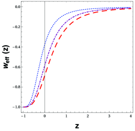
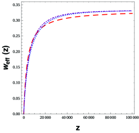
In Fig. 1, we plot for the energy balance obtained by the best fit of and (see subsections 4.1 and 4.2 below). As expected when , while for [40]. When compared with the CDM model with the same ’s and CMB+BAO+SNIa combined data are used, our model fits better for small and approaches faster to radiation dominated epoch when increases.
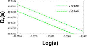
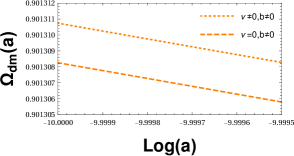
It is worthwhile mentioning that the decay of the cosmological term into radiation which includes relativistic (in the very early Universe) matter, does not affect the nucleosynthesis process, as it can be seen in Fig. 2, where the abundance of the relativistic species, including usual (baryonic) matter is compared with the corresponding data of CDM case represented by . In this plot, we take again the best fit values given by using CMB+BAO+SNIa combined data, this is, for the cosmological constant running parameter and for the DM warmness.
3 Including perturbations
The cosmological perturbations in the model described above can be analyzed following the approach developed in Refs. [10] and [22]. This implies simultaneous perturbations of metric, energy density and the four-velocities in the co-moving coordinates,
| (24) |
in the synchronous gauge . Here is the DM velocity and is the usual, or baryonic, matter (radiation, in our case) velocity. In the following calculations we use the constraint .
The perturbation of the DM pressure should be derived from the equation of state (4),
| (25) |
meaning that the perturbations satisfy the same equation of state as the background quantities. Technically, this means that the variations of the energy density and the rest energy density are always proportional. The reason for this restriction is that in the framework of the RRG model one has to provide kinetic energies of all particles to be equal and, therefore, we have no right to change the ratio [22]. The definitions of the perturbations for other densities are straightforward.
Let us introduce useful notations for the quantities related to Eq. (22),
| (26) |
Thus, we arrive at the -component of Einstein equations,
| (27) |
where and
| (28) |
are the corresponding density contrasts. Equations corresponding to the time and spatial components of the perturbation for the conservation law , have the form
| (29) | |||
| (30) | |||
| (31) | |||
| (32) |
Here we used the notations and for divergences of the peculiar velocities and we rewrote all the previous perturbation equations in the Fourier space, using
| (33) |
Perturbing the formula (1), one finds
| (34) |
The last equation is not dynamical, representing a constraint that can be replaced into other equations. Using (34) in (27), (29), and (30), we arrive at the equations
| (35) | |||
| (36) | |||
| (37) |
The complete system of perturbation equations includes (31), (32), (35), (3) and (3).
4 Observational tests
The free parameters of the cosmological model for the early Universe with running cosmological constant and energy exchange between vacuum and matter can be constrained from various observational tests. Thus, the general framework of the model formulated above may have different applications (one can see e.g. [41] for the possibilities in a simpler model without cosmological constant running). As a first step, in the present section we consider the two tests, namely the position of the first acoustic peak of the CMB power spectrum and the inclusion of SNIa+BAO combined data.
Let us note that the process of cosmological constant decay into normal particles, as discussed in the previous sections, is effective in the primordial Universe, that is long before BBN. For this reason, we are allowed to use the transfer function in the usual standard format. However, this process leaves traces for the later epochs of the Universe evolution, encoded in the values of parameters and . In this way, one can use the tests from the late phase of the Universe for exploring the effect of running cosmological constant in the earlier epoch.
The statistical analysis of the data starts with the functions, constructed according to the general expression
| (38) |
where is the total number of observational data, are the theoretical predictions depending on free parameters , and represent the observational values with an error bar given by . In our case the free parameters are , and . Let us remember that defines the running of the vacuum energy, while and describe the DM relative density and warmness. As usual, . It is worth mentioning that here we are dealing with the late Universe, hence usual matter (baryonic) and radiation contents are separated.
The probability distribution function is constructed from as
| (39) |
where is a normalization constant.
4.1 The first CMB peak
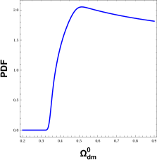
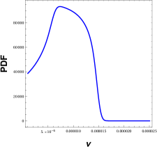
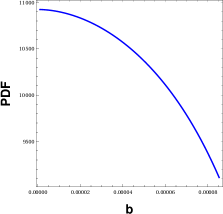
The position of the first peak in the CMB spectrum is related to the acoustic scale by the relation
| (40) |
with is evaluated at the redshift of the last scattering surface, [42]. The acoustic scale is defined by
| (41) |
where is the sound speed
| (42) |
Here and stand for the present density parameters of usual (baryonic) matter and photons, respectively. The relation (40) does not depend on the dark energy model. Here we consider the estimate and we use the values , and with the reduced Hubble constant [43]. Furthermore, we let the free parameters run in the intervals , and . The minimization of the statistics is done according to
| (43) |
where this function has a local minimum around
| (44) |
Here we can see that the current DM energy density value is higher than expected, indicating the necessity of a more robust observational test to get a better fit with respect to the standard model of cosmology (see Sec. 4.2).
It is easy to note that the value of quoted in (44) is dramatically different from the optimized value in CDM. Certainly, this is not what should be expected taking the relatively small values of DM warmness and running into account. Indeed, the difference can be understood by the fact that it corresponds only to the one particular observable, namely the first CMB peak. In this special situation, (that indicates a WDM) implies that more matter is required to reproduce the observed matter agglomeration. In what follows, we will use a more complete set of the observational data. Then the lower values for and will be obtained, implying also a lower value for , much closer to the conventional optimized value. In particular, taking both and equal to zero, the usual CDM results are obtained.
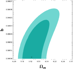
In Fig. 3 one can see the results for the one-dimensional marginalized probability distribution (PDF) for the free parameters of the model. It is easy to see that this test alone cannot constraint too much the parameters. Furthermore, the two-dimensional probability distribution, with both parameters being varied and one is integrated out, is shown in Fig. 4. The regions of higher probabilities in these plots are indicated by brighter tons.


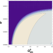
The PDF distribution shown in this sub-section does not cover a compact and finite domain in the parameter space. This output of the numerical analysis is due to two reasons. First of all, it is due to the physical restriction on the parameters of the model which we imposed. For example, we assumed that both and should be positive and cannot be either negative, neither greater than a threshold value. Certainly, from the statistical point of view, this is odd, and hence we can not be surprised by the unconventional form of the region in the parameter space.
Second, it is known that for some specific models, a given parameter may have a non-negligible PDF for disjoint regions. Even if such a feature may look unusual, it can be found in the literature. One particular example is the predictions for the equation of state parameter of the Generalised Chaplygin gas, where the constraints from the Integrated Sachs-Wolfe (ISW) effect implies either or , with the limit giving results similar to [59].
4.2 Including BAO and SNIa data
To find better constraints for our free parameters, in this section it is constructed a more robust test using SNIa and BAO combined data. Thus, we shall use
| (45) |
where and are constructed following the reference [44]. The results of this test are summarized in Table 2 and are given by
| (46) |
Note that this is lower than the previous estimate (44) and therefore looks closer to the constraints obtained with the CDM model. It is also important to note that in this combined test, it was used , instead of as in section 2. Additionally, we observe considerable variations in and values.
| Parameter | SNIa | SNIa+BAO | SNIa+BAO+CMB |
|---|---|---|---|
| 562.227 | 583.289 | 585.440 | |
| 0.261 | 0.275 | 0.308 | |
| 0.680 | 0.647 | 0.656 | |
| AIC | 566.227 | 587.289 | 589.440 |
| BIC | 587.679 | 608.823 | 610.981 |
| Parameter | SNIa | SNIa+BAO | SNIa+BAO+CMB |
|---|---|---|---|
| 562.315 | 583.402 | 585.374 | |
| 0.263 | 0.291 | 0.321 | |
| 1.970 | 3.149 | 2.442 | |
| 1.170 | 1.870 | 1.888 | |
| AIC | 568.315 | 589.402 | 591.374 |
| BIC | 600.493 | 621.703 | 623.685 |
| Parameter | SNIa | SNIa+BAO | SNIa+BAO+CMB |
|---|---|---|---|
| AIC | 2.088 | 2.113 | 1,934 |
| BIC | 12.814 | 12.880 | 12.704 |
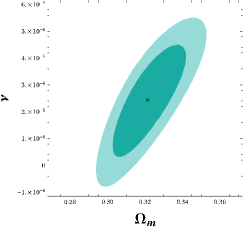
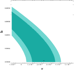
On the other hand, in Tables 1 and 3 we have written the best fit values for CDM () as our reference frame and the comparative analysis between both models. Two of the main statistical criteria to select models is the Akaike Information Criterion (AIC) [45], and the Bayesian Information Criterion (BIC) [46], defined respectively by, and , where is the number of degree of freedom and the number of observational data. These criteria take into account the number of free parameters of each model since the general tendency of models of higher number of free parameters is to fit better the data. Frequently it is used on the Jeffreys scale [47] to quantify the relativity statistical relevance of the models. For the AIC (BIC) parameter, models such have strong support, weak support in the case and are disfavored for . From table 3 the Jeffreys scale applied to the AIC statistical criterion favors the model RRG+RGE, while this model is strongly disfavored using the BIC criterium, a consequence of the large number of observational data, specially the SNIa data. This discrepancy in using the two criteria is a common feature found in the literature [48]-[50]. The contourplots with 1 and 2 levels for the CMB+BAO+SNIa combined data are shown in Fig. 5.
Let us note that the fact that the most probable values (44) and (46) include does not constitute proof of the running of the cosmological constant. As usual, the statistics with an extra free parameter, such as , always gives the best values for the non-zero parameter, and this is what we observe here. At the same time, it is remarkable that letting cosmological constant run does not lead to dramatic changes in the best fit for other parameters, such as DM relative density and the warmness .
4.3 Matter power spectrum
The matter power spectrum at is given by
| (47) |
where is a normalization constant of the spectrum. This constant can be fixed from the spectrum of anisotropy of the CMB radiation and
| (48) |
Here we use the Bardeen-Bond-Kaiser-Szalay (BBKS) transfer function [51]
| (49) |
where
| (50) |
to construct a set of initial conditions for the system of equations (31), (32), (35)-(3).
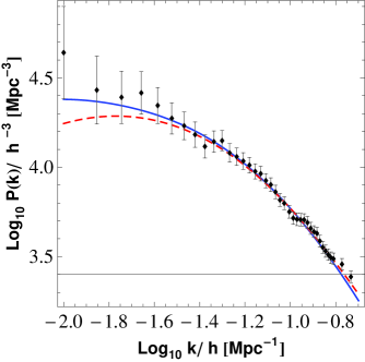
In Fig. 6 we compare the data from the 2dFGRS survey [52] with the matter power spectrum of our model for the energy balance obtained by the best fit of (see Table 2). Compared to more recent surveys (see e.g. [53]), the 2dFGRG data present the advantage of being less contaminated by the standard model used in the calibration.
5 Conclusions
We have implemented the model for the running of the cosmological constant in an early stage of the Universe, where the dark matter sector is modeled using the reduced relativistic gas model. At the background level, the model was solved analytically, taking into account the energy exchange between vacuum energy and usual (baryonic) matter. The effective equation of state parameter evolves as expected and we find the best fit with respect to the standard model, once the constrained values using SNIa+BAO+CMB combined data are obtained. Additionally, this effective parameter goes to radiation value faster than in the standard model for large redshift . Besides the first CMB peak, the SNIa and BAO data are used for constraining our free parameters,obtaining a better correspondence with observations for this case.
On the other hand, when considering perturbations, to compute the matter power spectrum, the system of equations for the geometric perturbation, density contrasts, and velocities are found and solved numerically. We compared our results with the ones of the 2dFRG data, obtaining a better correspondence for small , in contrast to the standard CDM model.
Our results suggest that a primordial running of the cosmological constant and the possible creation of usual (baryonic) matter particles at this early stage from vacuum energy, cannot be ruled out and deserves more detailed exploration, e.g. in the possible future work.
The model which we developed here explores the possibility that the cosmological term decays into the baryonic component in the early Universe, when the running of the cosmological constant and the intensity of the gravitational field are sufficiently strong and, on the other hand, baryonic matter contents can be regarded as ultra-relativistic particles. The parameter indicates a non-constant cosmological term and the parameter parameterizes the warmness of the matter component.
The comparison with observation points to a small deviation from the CDM model as the preferred scenario, even though the strict CDM case, given by , is not excluded. It must be remembered also that the running of the cosmological term implies a new free parameter in comparison to the standard cosmological model and, therefore, the results can not be interpreted such that the statistical analysis proves that the cosmological constant runs. Furthermore, the warmness of the dark matter component is allowed, with a present-day average speed of the corresponding particles (or indefinite origin, as usual) of the order of .
Finally, let us stress the similarities and, on the other hand, conceptual and technical differences between the model of running cosmology which we dealt with in this work and the purely phenomenological models describing the variable Dark Energy. The model developed in this paper belongs to the class of interaction models, where the energy-momentum tensor for some components does not conserve separately as it happens in the Standard Model. This means that a given component decays into another one. This class of interacting model is nowadays very popular in the study of the dark sector of the Universe, addressing some questions like the coincidence problem. However, the framework assumed here is quite different from most of these papers. In the first place, we deal with an interacting model for the early Universe, instead of a model for the late Universe. In the present case, the (dynamical) cosmological term decays into the usual (baryonic) matter when it is in the ultra-relativistic regime. On the other hand, the form of the -dependence for the cosmological constant density in our model is defined from the quantum field theory arguments [5, 6, 4]. These arguments defined the form of the IR running (1), leaving the unique arbitrariness in the coefficient .
From the technical side, it is interesting to see whether some known phenomenological models describe an energy exchange between vacuum and matter, like the one we considered here. Since there are numerous models of this sort, the complete analysis is beyond our possibilities, so we mention only one particular example. There is some similarity with the model developed earlier in Refs. [57, 58] where it was considered the energy exchange between vacuum and radiation, through the evaporation of primordial black hole. In those references the form of decaying of the cosmological term was fixed as an exponential decay, leading to a smooth transition from inflation to a radiation dominated phase, but with a prediction for the spectral index of scalar perturbations was found to contradict the observational constraints. This problem can be solved on the base of Eq. (1), by imposing upper bounds on the coefficient . On the other hand, the comparison with the scenario described above is not direct since we consider a pos-inflationary phase in contrast with the case treated in the mentioned references.
Acknowledgements
Authors are very grateful to Prof. A.A. Starobinsky for useful critical observations. J. A. Agudelo Ruiz thanks Prof. O.F. Piattella for useful discussions during the lecture course on cosmology at UFES and to A. Bonilla for his comments and discussion about data analysis and statistics. He is also grateful to CAPES for supporting his Ph.D. project. T.P.N. is grateful to CAPES for partial support and to the Núcleo Cosmo-UFES and PPGCosmo for kind hospitality and support during his visit at the Universidade Federal do Espírito Santo, where part of this work was done. The work of J.F. was partially supported by Fundação de Amparo à Pesquisa e Inovação do Espírito Santo - FAPES and by the Conselho Nacional de Desenvolvimento Científico e Tecnológico - CNPq. I.Sh. was partially supported by Conselho Nacional de Desenvolvimento Científico e Tecnológico - CNPq under the grant 303635/2018-5 and Fundação de Amparo à Pesquisa de Minas Gerais - FAPEMIG, under the project APQ-01205-16.
References
- [1] R. Utiyama and B.S. DeWitt, Renormalization of a classical gravitational field interacting with quantized matter fields, J. Math. Phys. 3 (1962) 608.
- [2] B.L. Nelson and P. Panangaden, Scaling Behavior Of Interacting Quantum Fields In Curved Space-Time, Phys.Rev. D25 (1982) 1019.
- [3] I.L. Buchbinder, S.D. Odintsov and I.L. Shapiro, Effective Action in Quantum Gravity (IOP Publishing, Bristol, 1992).
- [4] I.L. Shapiro, Effective Action of Vacuum: Semiclassical Approach, Class. Quant. Grav. 25 (2008) 103001, arXiv:0801.0216.
- [5] I.L. Shapiro, J. Solà, The scaling evolution of the cosmological constant, JHEP 02 (2002) 006.
- [6] I.L. Shapiro and J. Solà, On the possible running of the cosmological “constant” Phys. Lett. B682 (2009) 105, arXiv:0910.4925.
- [7] I.L. Buchbinder, On renormalization group equations in curved space-time. Theor. Math. Phys. 61 (1984) 393.
- [8] E.V. Gorbar, I.L. Shapiro, Renormalization Group and Decoupling in Curved Space. JHEP 02 (2003) 021; hep-ph/0210388.
- [9] I.L. Shapiro, J. Solà, C. España-Bonet, P. Ruiz-Lapuente, Variable cosmological constant as a Planck scale effect, Phys. Lett. 574B (2003) 149, astro-ph/0303306.
- [10] J. C. Fabris, I. L. Shapiro, J. Solà, Density Perturbations for Running Cosmological Constant, JCAP 0702 (2007) 016, gr-qc/0609017.
- [11] J. Solà, Cosmological constant and vacuum energy: old and new ideas, J. Phys. Conf. Ser. 453 (2013) 012015, arXiv:1306.1527.
- [12] S. Basilakos, N. E. Mavromatos and J. Solà, Do we come from a quantum anomaly?. Int. J. Mod. Phys. 28 (2019) 1944002 arXiv:1905.04685.
- [13] S. Basilakos, N. E. Mavromatos and J. Solà, Gravitational and chiral anomalies in the running vacuum Universe and matter-antimatter asymmetry, arXiv:1907.04890.
- [14] J. Grande, J. Solà, J.C. Fabris and I.L. Shapiro, Cosmic perturbations with running G and Lambda, Class. Quantum Grav. 27 (2010) 105004, arXiv:1001.0259.
- [15] D.C. Rodrigues, P.S. Letelier and I.L. Shapiro, Galaxy rotation curves from General Relativity with Renormalization Group corrections, JCAP 1004 (2010) 020, arXiv:0911.4967.
- [16] D.C. Rodrigues, S. Mauro and Á.O.F. de Almeida, Solar System constraints on Renormalization Group extended General Relativity: The PPN and Laplace-Runge-Lenz analyses with the external potential effect, Phys. Rev. D94 (2016) 084036, arXiv:1609.03613.G318
- [17] A.A. Starobinski, A new type of isotropic cosmological models without singularity, Phys. Lett. B91 (1980) 99.
- [18] A.A. Starobinsky, The perturbation spectrum evolving from a nonsingular initially de-Sitter cosmology and the microwave background anisotropy, Sov. Astron. Lett. 9 (1983) 302.
- [19] R. Opher and A. Pelinson, Studying the decay of the vacuum energy with the observed density fluctuation spectrum, Phys. Rev. D70 (2004) 063529, astro-ph/0405430; Decay of the vacuum energy into CMB photons, Mon. Not. Roy. Astron. Soc. 362 (2005) 167, astro-ph/0409451.
- [20] A. D. Sakharov, The initial stage of an expanding Universe and the appearance of a nonuniform distribution of matter, Sov. Phys. JETP 22 (1966) 241.
- [21] G. de Berredo-Peixoto, I. L. Shapiro and F. Sobreira, Simple cosmological model with relativistic gas, Mod. Phys. Lett.A20 (2005) 2723, gr-qc/0412050.
- [22] J. C. Fabris, I. L. Shapiro and F. Sobreira, DM particles: how warm they can be?, JCAP 0902 (2009) 001, arXiv:0806.1969.
-
[23]
A. Babic, B. Guberina, R. Horvat and
H. Stefancic,
Renormalization group running of the cosmological constant and its
implication for the Higgs boson mass in the standard model,
Phys. Rev. D65 (2002) 085002;
(2003) 083001;
B. Guberina, R. Horvat and H. Stefancic, Renormalization group running of the cosmological constant and the fate of the universe, Phys. Rev. D67 (2003) 083001, hep-ph/0211184. - [24] I. L. Shapiro, J. Solà and H. Stefancic, Running and at low energies from physics at MX: possible cosmological and astrophysical implications, JCAP 0501 (2005) 012, hep-ph/0410095.
- [25] E.V. Gorbar, I.L. Shapiro, Renormalization Group and Decoupling in Curved Space: II. The Standard Model and Beyond. JHEP 06 (2003) 004, hep-ph/0303124.
-
[26]
S.A. Franchino-Viñas, T. de Paula Netto, I.L. Shapiro
and O. Zanusso,
Form factors and decoupling of matter fields in four-dimensional
gravity,
Phys. Lett. B790 (2019) 229,
arXiv:1812.00460;
S. A. Franchino-Viñas, T. de Paula Netto and O. Zanusso, Vacuum effective actions and mass-dependent renormalization in curved space, Universe 5 (2019) 67, arXiv:1902.03167. - [27] A. Babic, B. Guberina, R. Horvat and H. Stefancic, Renormalization-group running cosmologies. A Scale-setting procedure, Phys. Rev. D71 (2005) 124041, astro-ph/0407572.
- [28] S. Domazet and H. Stefancic, Renormalization group scale-setting in astrophysical systems, Phys. Lett. B703 (2011) 1, arXiv:1010.3585.
- [29] N.R. Bertini, W.S. Hipólito-Ricaldi, F. de Melo-Santos and D.C. Rodrigues, Cosmological framework for renormalization group extended gravity at the action level, Eur. Phys. J. C80 (2020) 479, arXiv:1908.03960.
- [30] C. Farina, W.J.M. Kort-Kamp, S. Mauro and I.L. Shapiro, Dynamics of the Laplace-Runge-Lenz vector in the quantum-corrected Newton gravity, Phys. Rev. D83 (2011) 124037, arXiv:1101.5611.
-
[31]
M. Szydlowski and A. Stachowski,
Cosmological models with running cosmological term and
decaying dark matter,
Phys. Dark Univ. 15 (2017) 96, arXiv:1508.05637;
M. Szydlowski, A. Stachowski, K. Urbanowski, The evolution of the FRW universe with decaying metastable dark energy – a dynamical system analysis, JCAP 04 (2020) 029, arXiv:1812.00616;
M. Szydlowski and A. Stachowski, Cosmology with decaying cosmological constant – exact solutions and model testing, JCAP 10 (2015) 066, arXiv:1507.02114. - [32] https://demonstrations.wolfram.com/FittingAnElephant/
- [33] F. Jttner, Das Maxwellsche Gesetz der Geschwindigkeitsverteilung in der Relativtheorie, Ann. der Phys. Bd 116 (1911) S. 145.
- [34] R. Adam et al. Planck 2015 results-I. Overview of products and scientific results, Astronomy & Astrophysics 594 (2016): A1.
- [35] S. Castardelli dos Reis and I.L. Shapiro. Cosmic anisotropy with Reduced Relativistic Gas, Eur. Phys. J. C78 (2018) 145, arXiv:1712.03066.
- [36] G. Pordeus-da-Silva, R.C. Batista and L.G. Medeiros, Theoretical foundations of the reduced relativistic gas in the cosmological perturbed context, JCAP 2019 (2020) 043, arXiv:1904.09904.
- [37] J.C. Fabris, A.M. Velasquez-Toribio, W. Zimdahl and I.L. Shapiro, Interacting photon-baryon fluid, warm dark matter and the first acoustic peak, Eur. Phys. J. C74 (2014) 2968, arXiv:1312.1937.
- [38] W. S. Hipólito-Ricaldi, R. F. Marttens, J. C. Fabris, I. L. Shapiro and L. Casarini, On general features of warm dark matter with reduced relativistic gas, Eur. Phys. J. C 78 (2018) 365, arXiv:1706.08595.
- [39] C. Espana-Bonet, P. Ruiz-Lapuente, I. L. Shapiro and J. Solà, Testing the running of the cosmological constant with type Ia supernovae at high z, JCAP 0402 (2004) 006, hep-ph/0311171.
- [40] A. Melchiorri et al. The state of the dark energy equation of state, Phys. Rev. D68 (2003) 043509.
- [41] J. C. Fabris, I. L. Shapiro and A. M. Velasquez-Toribio, Testing dark matter warmness and quantity via the reduced relativistic gas model, Phys. Rev. D85, 023506 (2012), arXiv:1105.2275.
- [42] W. Hu and N. Sugiyama. Anisotropies in the cosmic microwave background: An Analytic approach, Astrophys. J. 444 (1995) 489, astro-ph/94070.
- [43] Akrami, Y., et al. Planck 2018 results. I. Overview and the cosmological legacy of Planck. arXiv:1807.06205 (2018).
- [44] A. Bonilla Rivera and J. E. García-Farieta, Exploring the Dark Universe: constraints on dynamical Dark Energy models from CMB, BAO and growth rate measurements, Int. J. Mod. Phys. D28 (2019) 1950118, arXiv:1605.01984.
- [45] Akaike, H. ”A new look at the statistical model identification, IEEE T. Automat. Contr., 19, 716–723.” Go to original source (1974).
- [46] Schwarz, Gideon. ”Estimating the dimension of a model.” The annals of statistics 6.2 (1978): 461-464.
- [47] Liddle, Andrew R. ”Information criteria for astrophysical model selection.” Monthly Notices of the Royal Astronomical Society: Letters 377.1 (2007): L74-L78.
- [48] Szydlowski, Marek, and Aleksandra Kurek. AIC, BIC, Bayesian evidence and a notion on simplicity of cosmological model. No. arXiv: 0801.0638. 2008.
- [49] Del Campo, Sergio, et al. ”Holographic dark-energy models.” Physical Review D 83.12 (2011): 123006.
- [50] Szydlowski, Marek, et al. ”AIC, BIC, Bayesian evidence against the interacting dark energy model.” The European Physical Journal C 75.1 (2015): 5.
- [51] J.M. Bardeen, J.R. Bond, N. Kaiser and A.S. Szalay, The Statistics of Peaks of Gaussian Random Fields, Astrophys. J. 304 (1986) 15.
- [52] 2dFGRS collaboration, S. Cole et al., The 2dF Galaxy Redshift Survey: Power-spectrum analysis of the final dataset and cosmological implications, Mon. Not. Roy. Astron. Soc. 362 (2005) 505, astro-ph/0501174.
- [53] D. Parkinson et al., The WiggleZ Dark Energy Survey: Final data release and cosmological results, Phys. Rev. D86 (2012) 103518, arXiv:1210.2130.
- [54] F. Juttner, Die dynamik eines bewegten gases in der relativtheorie, Annalen der Physik 6, 145 (1911).
- [55] R. R. Caldwell, R. Dave and P. J. Steinhardt, Cosmological imprint of an energy component with general equation of state, Phys. Rev. Lett. 80 (1998) 1582, astro-ph/9708069.
- [56] V. Gorini, A.Y. Kamenshchik, U. Moschella and V. Pasquier, Tachyons, scalar fields and cosmology, Phys. Rev. D69 (2004) 123512, hep-th/0311111.
- [57] J.C. Fabris and Ph. Spindel, Scalar perturbations in a primordial inflationary scenario, Phys. Rev. D64 (2001) 084007, hep-th/0104040.
- [58] Ph. Spindel and R. Brout, Entropy production from vacuum decay, Phys. Lett. B320 (1994) 241, gr-qc/9310023.
- [59] O.F. Piattella, The extreme limit of the generalized Chaplygin gas, JCAP 1003(2010) 012, arXiv:0906.4430.