Tolman lengths and rigidity constants from free-energy functionals – General expressions and comparison of theories

Abstract

The leading order terms in a curvature expansion of the surface tension, the Tolman length (first order), and rigidities (second order) have been shown to play an important role in the description of nucleation processes. This work presents general and rigorous expressions to compute these quantities for any non-local density functional theory (DFT). The expressions hold for pure fluids and mixtures, and reduce to the known expressions from density gradient theory (DGT). The framework is applied to a Helmholtz energy functional based on the perturbed chain polar statistical associating fluid theory (PCP-SAFT) and is used for an extensive investigation of curvature corrections for pure fluids and mixtures. Predictions from the full DFT are compared to two simpler theories: predictive density gradient theory (pDGT), that has a density and temperature dependent influence matrix derived from DFT, and DGT, where the influence parameter reproduces the surface tension as predicted from DFT. All models are based on the same equation of state and predict similar Tolman lengths and spherical rigidities for small molecules, but the deviations between DFT and DGT increase with chain length for the alkanes. For all components except water, we find that DGT underpredicts the value of the Tolman length, but overpredicts the value of the spherical rigidity. An important basis for the calculation is an accurate prediction of the planar surface tension. Therefore, further work is required to accurately extract Tolman lengths and rigidities of alkanols, because DFT with PCP-SAFT does not accurately predict surface tensions of these fluids.

I Introduction

The dependence of the surface tension on the interfacial curvature has been discussed intensely over the last decades. One of the motivations for studying the subject was the discrepancies between experiments and theoretical predictions for nucleation rates in condensation and evaporation Iland et al. (2007); Vehkamäki (2006). In classical nucleation theory, the nucleation rate depends exponentially on the formation energy of the nano-sized critical cluster. Therefore, it has been hypothesized that omitting the curvature dependence of the surface tension is the cause of the large discrepancies between theory and experiments Vehkamäki (2006); ten Wolde and Frenkel (1998); Wilhelmsen, Bedeaux, and Reguera (2015a); Nguyen et al. (2018). The curvature dependence of the surface tension also has implications for other important examples such as the properties of biomembranesHelfrich (1973), and wetting at the nanoscaleKim et al. (2018).

The first quantitative description was proposed by TolmanTolman (1949). By introducing the distance between the equimolar radius $R_{e}$ and the radius of the surface of tension $R_{s}$, referred to as $\delta_{T}(R_{s})$, he proposed the expression

$$\sigma(R_{s})=\frac{\sigma_{0}}{1+\frac{2\delta_{T}(R_{s})}{R_{s}}},$$ (1)

for the curvature dependent surface tension $\sigma(R_{s})$ in relation to the surface tension of a planar interface $\sigma_{0}$. In Eq. (1), the curvature dependent Tolman length, $\delta_{T}(R_{s})$ is often replaced by the Tolman length of the planar interface $\delta$. In later works Wilhelmsen, Bedeaux, and Reguera (2015a, b); Bruot and Caupin (2016); Aasen, Blokhuis, and Wilhelmsen (2018); Rehner and Gross (2018a), it was shown that with this approximation, Eq. (1) is incapable of representing the surface tension of small droplets. Instead, the second-order expression by HelfrichHelfrich (1973) has been established as the preferred model to capture the curvature dependence of the surface tension. For an arbitrarily curved interface, it reads

$$\sigma(J,K)=\sigma_{0}-\delta\sigma_{0}J+\frac{k}{2}J^{2}+\bar{k}K+\ldots,$$ (2)

where $\delta$ is the the Tolman length, $k$ is the bending rigidity and $\bar{k}$ is the Gaussian rigidity. The interface is characterized locally by the total curvature $J=1/R_{1}+1/R_{2}$ and the Gaussian curvature $K=1/\left(R_{1}R_{2}\right)$, with $R_{1}$ and $R_{2}$ being the two principal radii. The expansion truncated at second order is known as the Helfrich expansion, and the coefficients $\sigma_{0}$, $\delta$, $k$ and $\bar{k}$ are referred to as Helfrich coefficients. For spherical (index $s$) and cylindrical (index $c$) geometries, Eq. (2) simplifies to

$$\sigma^{s}(R) =\sigma_{0}-\frac{2\delta\sigma_{0}}{R}+\frac{2k+\bar{k}}{R^{2}}+\ldots~{}~{}~{}~{}~{}~{}\text{and}$$ (3)

$$\sigma^{c}(R) =\sigma_{0}-\frac{\delta\sigma_{0}}{R}+\frac{k}{2R^{2}}+\ldots$$ (4)

where $R$ is an arbitrarily chosen dividing surface. The Tolman length for the vapor–liquid interface has been the subject of many discussions and controversies, in particular its sign, since different routes to obtain it have yielded different results. Due to its simplicity, most works in the literature have considered the truncated and shifted Lennard–Jones (LJ) fluid. Theoretical calculations based on free-energy functionals of the density profile, such as density gradient theory (DGT) and non-local density functional theory (DFT), have consistently given zero or negative values Blokhuis and Kuipers (2006); Li and Wu (2007); Block et al. (2010); Tröster et al. (2012). However, positive values have been reported from Monte Carlo and molecular dynamics (MD) simulations that compute the Tolman length from the pressure tensor (see van Giessen and Blokhuis (2002); Lei et al. (2005); Horsch et al. (2012) and references therein). MD simulations by van Giessen and Blokhuis, and also by Block et al. have only recently resulted in negative Tolman lengths around $-0.1$ in units of the LJ diameter van Giessen and Blokhuis (2009); Sampayo et al. (2010); Block et al. (2010); a consensus on this value is emerging in the scientific community Blokhuis and van Giessen (2013). Curvature corrections for water have also been investigated intenselyWilhelmsen, Bedeaux, and Reguera (2015a); Menzl et al. (2016); Joswiak et al. (2013, 2016); Kanduč (2017); Kim et al. (2018); Leong and Wang (2018), also with conflicting results on the sign of the Tolman length. Still, DGT and DFT have been shown to agree quantitatively with the predictions of recent simulation studies for both the LJ fluidvan Giessen and Blokhuis (2009); Blokhuis and van Giessen (2013); Wilhelmsen, Bedeaux, and Reguera (2015b) and waterWilhelmsen, Bedeaux, and Reguera (2015a); Joswiak et al. (2013, 2016); Kanduč (2017), giving credibility to DFT and DGT as methodologies to calculate curvature corrections.

Free-energy functionals allow direct calculation of the curvature dependence of the surface tension. In principle, the unknown coefficients in Eqs. (3) and (4) can be estimated by fitting a second order polynomial of the surface tension as a function of the curvature, $1/R$ Rehner and Gross (2018a). Since the surface tension of large droplets and bubbles is very similar to $\sigma_{0}$, coefficients computed in this manner have limited accuracy. A more accurate and rigorous route is to directly calculate the derivatives of the surface tension with respect to curvature from the free-energy functional Fisher and Wortis (1984). This involves solving for the first-order curvature expansion of the density profiles. The methodology was first presented by Blokhuis and Bedeaux for pure fluids described by DGT Blokhuis and Bedeaux (1993), and later extended to mixtures described by DGT by Aasen et al Aasen, Blokhuis, and Wilhelmsen (2018). Estimates of the Helfrich coefficients have also been computed from various other free-energy functionalsvan Giessen, Blokhuis, and Bukman (1998); Barrett (2009); Blokhuis and van Giessen (2013); Rehner and Gross (2018a). Still, a robust method for calculating these coefficients rigorously from arbitrary free-energy functionals and a systematic comparison of the values derived from different functionals for a range of fluids is missing.

This work presents general expressions to compute the Tolman length and rigidity constants for arbitrary free-energy functionals, that hold for pure fluids and mixtures. These expressions are next applied to predict the Helfrich coefficients to state-of-the-art accuracy for a range of pure fluids and mixtures, using a non-local DFT based on the perturbed-chain polar statistical associating fluid theory (PCP-SAFT) equation of state. We present the first systematic comparison of these coefficients to predictions from DGT and predictive density gradient theory (pDGT) Rehner and Gross (2018b). The comparison yields insight into the limits of using gradient theories for the description of curved interfaces. We will also shed light on the impact of the underlying equation of state in DGT and non-local DFT.

In section II we develop the general expressions for the Helfrich coefficients, valid for any free-energy functional. In sections III.1 and III.2, coefficients for a range of pure fluids and mixtures are compared. In section IV, we offer some concluding remarks.

II Theory

In this section we first review the general model-independent relations appearing in the curvature expansion. Subsequently we present the new expressions for the Helfrich coefficients for non-local DFT and shed light on how to treat the density dependence of the influence parameter in predictive density gradient theory. In all expressions, we consider isothermal conditions and paths. Bold symbols denote vector properties with respect to the components in the system.

II.1 General relations for curvature expansion

The aim of a curvature expansion is to determine thermodynamic properties of a curved interface by Taylor expanding around the planar interface. Therefore, every property $X$ that depends on the curvature is written as

$$X=X_{0}+\frac{X_{1}}{R}+\frac{X_{2}}{R^{2}}+\ldots,$$ (5)

where the coefficients $X_{i}$ do not depend on the curvature. To be able to describe an arbitrarily shaped interface using the Helfrich expansion, the curvature expansion has to be performed in spherical and cylindrical coordinates. In the following, we derive expressions that are valid for both geometries, captured by the geometry factor $g$, which is 0 for a planar interface, 1 for a cylindrical interface and 2 for a spherical interface. Before presenting model-specific expressions, we derive general relations between the different properties of curved interfaces.

Gibbs–Duhem equation

The bulk pressures in the liquid ($L$) and the vapor ($V$) phase are related to the chemical potential $\bm{\mu}$ and the density $\bm{\rho}$ of the system via the Gibbs-Duhem equation

$$\bm{\rho}^{V}\cdot\mathrm{d}\bm{\mu}=\mathrm{d}p^{V} \bm{\rho}^{L}\cdot\mathrm{d}\bm{\mu}=\mathrm{d}p^{L}.$$ and (6)

Thus, the pressure difference $\Delta p=p^{L}-p^{V}$ is linked to the difference in densities $\Delta\bm{\rho}=\bm{\rho}^{L}-\bm{\rho}^{V}$ via

$$\Delta\bm{\rho}\cdot\mathrm{d}\bm{\mu}=\mathrm{d}\Delta p.$$ (7)

Using Eq. (5) for all properties leads to the expression

$$\left(\Delta\bm{\rho}_{0}+\frac{\Delta\bm{\rho}_{1}}{R}+\ldots\right)\cdot\left(\bm{\mu}_{1}+\frac{2\bm{\mu}_{2}}{R}+\ldots\right)\mathrm{d}\left(\frac{1}{R}\right)=\\ \left(\Delta p_{1}+\frac{2\Delta p_{2}}{R}+\ldots\right)\mathrm{d}\left(\frac{1}{R}\right).$$ (8)

Collecting terms with the same power of $R$ results in the relations

$$\Delta p_{1} =\Delta\bm{\rho}_{0}\cdot\bm{\mu}_{1}~{}~{}~{}~{}~{}~{}~{}~{}~{}~{}\text{and}$$ (9)

$$\Delta p_{2} =\Delta\bm{\rho}_{0}\cdot\bm{\mu}_{2}+\frac{1}{2}\Delta\bm{\rho}_{1}\cdot\bm{\mu}_{1}.$$ (10)

Adsorption

The adsorption, $\bm{\Gamma}$ refers to the amount of particles accumulated at the interface per surface area, and isdefined as

$$\bm{\Gamma}=\int\bm{\rho}^{E}(r)\left(\frac{r}{R}\right)^{g}\mathrm{d}r,$$ (11)

where we introduce the excess density

$$\bm{\rho}^{E}(r)=\bm{\rho}(r)-\bm{\rho}^{L}\Theta(R-r)-\bm{\rho}^{V}\Theta(r-R),$$ (12)

with the Heaviside step function $\Theta(r)$. By changing the integration variable to $z=r-R$ and again collecting terms of the same order in curvature, the following expansion coefficients

$$\bm{\Gamma}_{0} =\int\bm{\rho}_{0}^{E}(z)\mathrm{d}z,~{}~{}~{}~{}~{}~{}~{}~{}~{}~{}\text{and}$$ (13)

$$\bm{\Gamma}_{1} =\int\left(\bm{\rho}_{1}^{E}(z)+gz\bm{\rho}_{0}^{E}(z)\right)\mathrm{d}z$$ (14)

are obtained.

Gibbs adsorption equation

The Gibbs adsorption equation

$$\mathrm{d}\sigma=-\bm{\Gamma}\cdot\mathrm{d}\bm{\mu}+\left[\frac{\partial\sigma}{\partial R}\right]_{T,\bm{\mu}}\mathrm{d}R$$ (15)

links the adsorption to the surface tension $\sigma$. As we have not yet made a choice of dividing surface, the notional derivative, $\left[\frac{\partial\sigma}{\partial R}\right]_{T,\bm{\mu}}$ appears in the equation. The notial derivative describes the change in surface tension due to a change in the dividing surface, while keeping the physical system unaltered. The notional derivative also enters the general form of the Young-Laplace equation, as

$$\Delta p=\frac{g\sigma}{R}+\left[\frac{\partial\sigma}{\partial R}\right]_{T,\bm{\mu}}.$$ (16)

Substituting the notional derivative from Eq. (16) into (15) and expanding the resulting expression gives a general relation between the coefficients of the pressure difference and the surface tension, as

$$\Delta p_{0} =0,~{}~{}~{}~{}\Delta p_{1}=g\sigma_{0}~{}~{}~{}~{}\text{and}$$

$$\Delta p_{2} =-\bm{\Gamma}_{0}\cdot\bm{\mu}_{1}+(g-1)\sigma_{1}.$$ (17)

Density profiles

The density profile of an open system is obtained as a stationary point of the grand potential functional $\Omega$. Using a Legendre transform, the equilibrium condition can be formulated in terms of the functional derivative of the Helmholtz energy, $F$ instead

$$\left.\frac{\delta\Omega}{\delta\bm{\rho}(\mathbf{r})}\right|_{T,V,\bm{\mu}}=0~{}~{}\Leftrightarrow~{}~{}\left.\frac{\delta F}{\delta\bm{\rho}(\mathbf{r})}\right|_{T,V}=\bm{\mu}.$$ (18)

A curvature expansion of Eq. (18) gives

$$\bm{\mu}_{0} =\left(\frac{\delta F}{\delta\bm{\rho}(\mathbf{r})}\right)_{0},~{}~{}\text{and}$$ (19)

$$\bm{\mu}_{1} =\int\left(\frac{\delta^{2}F}{\delta\bm{\rho}(\mathbf{r})\delta\bm{\rho}(\mathbf{r}^{\prime})}\right)_{0}\bm{\rho}_{1}(\mathbf{r}^{\prime})\mathrm{d}\mathbf{r}^{\prime}.$$ (20)

The density profile of the planar interface and the first-order term in the curvature expansion of the density can be obtained by solving the above equations. It is not obvious from the general formulation how they should be solved. However, one important property can be derived. For free-energy functionals $F$, the expression

$$\int\left(\frac{\delta^{2}F}{\delta\bm{\rho}(\mathbf{r})\delta\bm{\rho}(\mathbf{r}^{\prime})}\right)_{0}\nabla\bm{\rho}_{0}(\mathbf{r}^{\prime})\mathrm{d}\mathbf{r}^{\prime}=\nabla\left(\frac{\delta F}{\delta\bm{\rho}(\mathbf{r})}\right)_{0}=0,$$ (21)

vanishes at equilibrium. It follows, that if $\bm{\rho}_{1}(\mathbf{r})$ is a solution of Eq. (20), $\bm{\rho}_{1}(\mathbf{r})+\varepsilon\nabla\bm{\rho}_{0}(\mathbf{r})$ is also a solution for any value of $\varepsilon$.

Surface tension

The surface tension is defined as the excess grand potential per surface area, $\sigma=\frac{\Omega^{E}}{A}$. Using the geometry factor $g$, it can be expressed as

$$\sigma=\int\left(f-\bm{\rho}\cdot\bm{\mu}+p^{LV}\right)\left(\frac{r}{R}\right)^{g}\mathrm{d}r$$ (22)

with the Helmholtz energy density, $f$ and the pressure of the bulk phases, $p^{LV}=p^{L}\Theta(r-R)+p^{V}\Theta(R-r)$, which is related to the adsorption via the Gibbs-Duhem equation. After a few simplification steps and identifying the excess grand potential density of the planar interface, $\Delta\omega_{0}=f_{0}-\bm{\rho}_{0}\cdot\bm{\mu}_{0}+p_{0}$, the resulting expressions for the coefficients are

$$\sigma_{0}= \int\Delta\omega_{0}\mathrm{d}z$$ (23)

$$\sigma_{1}= \int\left(f_{1}-\bm{\rho}_{1}\cdot\bm{\mu}_{0}\right)\mathrm{d}z+g\int\Delta\omega_{0}z\mathrm{d}z-\bm{\mu}_{1}\cdot\bm{\Gamma}_{0}$$ (24)

$$\sigma_{2}= \int\left(f_{2}-\bm{\rho}_{2}\cdot\bm{\mu}_{0}-\frac{1}{2}\bm{\rho}_{1}\cdot\bm{\mu}_{1}\right)\mathrm{d}z$$

$$+g\int\left(f_{1}-\bm{\rho}_{1}\cdot\bm{\mu}_{0}\right)z\mathrm{d}z+\frac{g(g-1)}{2}\int\Delta\omega_{0}z^{2}\mathrm{d}z$$

$$-\frac{g}{2}\bm{\mu}_{1}\cdot\int\bm{\rho}_{0}^{E}z\mathrm{d}z-\bm{\mu}_{2}\cdot\bm{\Gamma}_{0}-\frac{1}{2}\bm{\mu}_{1}\cdot\bm{\Gamma}_{1}$$ (25)

It is tempting to neglect the first term in both the first and second order expressions for the surface tension as we find

$$\int\left(f_{1}-\bm{\rho}_{1}\cdot\bm{\mu}_{0}\right)\mathrm{d}\mathbf{r}=\\ \iint\left(\left(\frac{\delta f(\mathbf{r})}{\delta\bm{\rho}(\mathbf{r}^{\prime})}\right)_{0}\cdot\bm{\rho}_{1}(\mathbf{r}^{\prime})-\left(\frac{\delta f(\mathbf{r}^{\prime})}{\delta\bm{\rho}(\mathbf{r})}\right)_{0}\cdot\bm{\rho}_{1}(\mathbf{r})\right)\mathrm{d}\mathbf{r}\mathrm{d}\mathbf{r}^{\prime}$$ (26)

which is strictly zero. However, in Eq. (24), the integration is over $z$. We have to take into account that the integration takes place in a curvilinear coordinate system, even if one is interested in the limit of zero curvature.

Path through the metastable region

Although the norms of the vectors $\bm{\mu}_{1}$ and $\bm{\mu}_{2}$ are fixed by Eqs. (9), (10) and (17), their directions represent degrees of freedom. Every point in the metastable region is defined by its temperature and chemical potentials. However, there is an infinite number of possible starting points on the phase envelope and paths towards the metastable point, which are each equipped with their own expansion coefficients. In a previous studyAasen, Blokhuis, and Wilhelmsen (2018), it was shown that a straight path (i.e. $\bm{\mu}_{2}\propto\bm{\mu}_{1}$) where the composition of the liquid phase $\bm{x}^{L}$ is kept constant in the first order term gives low errors in the expansion. To obtain the coefficients of the chemical potential for this choice of path, the first order coefficient of the total liquid density is calculated as

$$\rho^{L}_{1}=\frac{g\sigma_{0}}{\left(\bm{x}^{L}\right)^{T}\left(\bm{\mu}_{\rho}^{L}\right)_{0}\Delta\bm{\rho}_{0}},$$ (27)

from which the chemical potential,

$$\bm{\mu}_{1}=\rho_{1}^{L}\left(\bm{\mu}_{\rho}^{L}\right)_{0}\bm{x}^{L}$$ (28)

and the vapor partial densities,

$$\bm{\rho}_{1}^{V}=\left(\bm{\mu}_{\rho}^{V}\right)_{0}^{-1}\bm{\mu}_{1}$$ (29)

follow. The second order coefficient for the chemical potential can be derived from Eqs. (10) and (17) as

$$\bm{\mu}_{2}=\frac{(g-1)\sigma_{1}-\left(\bm{\Gamma}_{0}+\frac{1}{2}\Delta\bm{\rho}_{1}\right)\cdot\bm{\mu}_{1}}{g\sigma_{0}}\bm{\mu}_{1}.$$ (30)

Choice of dividing surface

The equations derived so far are valid for any choice of dividing surface. However, to be able to evaluate the expressions, a choice has to be made. The first option is the surface of tension $R_{s}$, for which the notional derivative of the surface tension vanishes. Thus, the usual form of the Young Laplace equation $\Delta p=\frac{g\sigma}{R_{s}}$ is valid and the Gibbs adsorption equation simplifies to

$$\sigma_{1}=-\bm{\mu}_{1}\cdot\bm{\Gamma}_{0} \sigma_{2}=-\bm{\mu}_{2}\cdot\bm{\Gamma}_{0}-\frac{1}{2}\bm{\mu}_{1}\cdot\bm{\Gamma}_{1}.$$ and (31)

The second important option is the equimolar dividing surface or its generalization to multicomponent mixtures, the Koenig surfaceKoenig (1950) $R_{k}$, which is defined by $\bm{\Gamma}\cdot\mathrm{d}\bm{\mu}=0$. As opposed to the surface of tension which is a state function, the Koenig surface is path dependent. For specific applications, one choice might be superior. However, it is important to keep in mind that neither the planar surface tension nor the Tolman length depend on the dividing surface and there are simple model-independent relations for the rigidity constants for different dividing surfacesAasen, Blokhuis, and Wilhelmsen (2018).

In the density profile of the planar interface, the dividing surface is fixed by finding any density profile that solves the zeroth order Euler–Lagrange equation and then shifting the $z$-axis by the position of the Koenig surface $z_{k0}$ or the surface of tension $z_{s0}$. The values for the two surfaces are given by

$$z_{k0}=\frac{\bm{\mu}_{1}\cdot\bm{\Gamma}_{0}}{g\sigma_{0}} z_{s0}=\frac{\sigma_{1}+\bm{\mu}_{1}\cdot\bm{\Gamma}_{0}}{g\sigma_{0}}.$$ and (32)

From these relations, we obtain an expression for the Tolman length

$$z_{k0}-z_{s0}=\frac{-\sigma_{1}}{g\sigma_{0}}=\delta.$$ (33)

With a similar procedure, the correct solution of the first order Euler–Lagrange equation is found by first finding any solution $\bm{\tilde{\rho}}_{1}(z)$ and then obtaining the actual solution as $\bm{\rho}_{1}(z)=\bm{\tilde{\rho}}_{1}(z)+\varepsilon\bm{\rho}_{0}^{\prime}(z)$ with

$$\varepsilon=\frac{2\bm{\mu}_{2}\cdot\bm{\Gamma}_{0}+\bm{\mu}_{1}\cdot\bm{\tilde{\Gamma}}_{1}}{g\sigma_{0}}$$ (34)

for the Koenig surface and

$$\varepsilon=\frac{\sigma_{2}+2\bm{\mu}_{2}\cdot\bm{\Gamma}_{0}+\bm{\mu}_{1}\cdot\bm{\tilde{\Gamma}}_{1}}{g\sigma_{0}}$$ (35)

for the surface of tension.

II.2 Non-local density functional theory

In non-local density functional theory (DFT), the Helmholtz energy $F[\bm{\rho}(\mathbf{r})]=\int f[\bm{\rho}(\mathbf{r})]\mathrm{d}\mathbf{r}$ and the Helmholtz energy density $f[\bm{\rho}(\mathbf{r})]$ are functionals of the density profiles $\bm{\rho}(\mathbf{r})$ of all components. In most DFT approaches, the Helmholtz energy density can be written as a function of any number of weighted densities $n_{\alpha}$. This includes functionals based on fundamental measure theory (FMT)Rosenfeld (1989), local and weighted density approximationsTarazona (1985) and mean-field theoryBlokhuis and van Giessen (2013). The weighted densities are obtained by convolving the density profile with corresponding weight functions, $\bm{\omega}_{\alpha}$ in three dimensions

$$n_{\alpha}(\mathbf{r})=\bm{\rho}\stackrel{{\scriptstyle 3D}}{{\otimes}}\bm{\omega}_{\alpha}=\int\bm{\rho}(\mathbf{r}-\mathbf{r}^{\prime})\cdot\bm{\omega_{\alpha}}(\mathbf{r}^{\prime})\mathrm{d}\mathbf{r}^{\prime},$$ (36)

where the sum in the inner product is over all components. To calculate the expansion coefficients, the curvature expansion of the convolution integral is required. This is straightforward for a spherical geometry, but significantly more tedious in cylindrical coordinates, as shown in Appendix A. The zeroth and first order expressions for the weighted densities can be written using one dimensional convolution integrals,

$$n_{\alpha 0} =\bm{\rho}_{0}\otimes\bm{\omega}_{\alpha}~{}~{}~{}~{}~{}~{}~{}\text{and}$$ (37)

$$n_{\alpha 1} =\bm{\rho}_{1}\otimes\bm{\omega}_{\alpha}-\frac{g}{2}\bm{\rho}_{0}\otimes\left(z\bm{\omega}_{\alpha}\right).$$ (38)

For the curvature expansion, the first

$$f_{1} =\sum_{\alpha}f_{\alpha 0}n_{\alpha 1}~{}~{}~{}~{}\text{and second}$$ (39)

$$f_{2} =\frac{1}{2}\sum_{\alpha}f_{\alpha 1}n_{\alpha 1}+\sum_{\alpha}f_{\alpha 0}n_{\alpha 2}$$ (40)

order coefficients of the Helmholtz energy density are required. Here,

$$f_{\alpha 0}=\left(\frac{\partial f}{\partial n_{\alpha}}\right)_{0} f_{\alpha\beta 0}=\left(\frac{\partial^{2}f}{\partial n_{\alpha}\partial n_{\beta}}\right)_{0}$$ and (41)

is shorthand for the zeroth order first and second partial derivatives of the Helmholtz energy density and $f_{\alpha 1}=\sum_{\beta}f_{\alpha\beta 0}n_{\beta 1}$ is the corresponding first order expression. The same concept as for the weighted densities is used to obtain the first and second order expressions for the Euler–Lagrange equation, giving

$$\bm{\mu}_{0} =\left(\frac{\delta F}{\delta\bm{\rho}}\right)_{0}=\sum_{\alpha}f_{\alpha 0}\otimes\bm{\omega}_{\alpha}~{}~{}~{}~{}~{}~{}~{}\text{and}$$ (42)

$$\bm{\mu}_{1} =\left(\frac{\delta F}{\delta\bm{\rho}}\right)_{1}=\sum_{\alpha}\left(f_{\alpha 1}\otimes\bm{\omega}_{\alpha}-\frac{g}{2}f_{\alpha 0}\otimes\left(z\bm{\omega}_{\alpha}\right)\right).$$ (43)

Using Eqs. (38), (39) and (42), the first term in the general expression (24) for $\sigma_{1}$ can be simplified as

$$\int \left(f_{1}-\bm{\rho}_{1}\cdot\bm{\mu}_{0}\right)\mathrm{d}z$$

$$=\int\sum_{\alpha}\Big{(}f_{\alpha 0}\left(\bm{\rho}_{1}\otimes\bm{\omega}_{\alpha}\right)-\frac{g}{2}f_{\alpha 0}\left(\bm{\rho}_{0}\otimes\left(z\bm{\omega}_{\alpha}\right)\right)$$

$$~{}~{}~{}~{}~{}~{}~{}~{}~{}~{}~{}~{}~{}~{}~{}~{}~{}~{}~{}~{}~{}~{}~{}~{}~{}~{}~{}~{}~{}~{}~{}~{}~{}~{}~{}~{}~{}~{}-\bm{\rho}_{1}\left(f_{\alpha 0}\otimes\bm{\omega}_{\alpha}\right)\Big{)}\mathrm{d}z$$

$$=-\frac{g}{2}\int\sum_{\alpha}f_{\alpha 0}\left(\bm{\rho}_{0}\otimes\left(z\bm{\omega}_{\alpha}\right)\right)\mathrm{d}z.$$

Through its definition $\sigma_{1}=-g\delta\sigma_{0}$, the Tolman length follows as

$$\delta\sigma_{0}=\frac{1}{2}\int\sum_{\alpha}f_{\alpha 0}\left(\bm{\rho}_{0}\otimes\left(z\bm{\omega}_{\alpha}\right)\right)\mathrm{d}z\\ -\int\Delta\omega_{0}z\mathrm{d}z+\frac{1}{2}\bm{\mu}_{1}^{s}\cdot\bm{\Gamma}_{0}.$$ (44)

For different Helmholtz energy functionals, the Tolman length depends only on the planar density profile Blokhuis and Bedeaux (1993); Blokhuis and van Giessen (2013). In a similar albeit more elaborate fashion, the rigidity constants are obtained as

$$k=-\frac{1}{4}\int\sum_{\alpha}f_{\alpha 0}\left(\bm{\rho}_{0}\otimes\tilde{\bm{\omega}}_{\alpha}\right)\mathrm{d}z\\ -\frac{1}{4}\int\sum_{\alpha}\left(\bm{\rho}_{1}^{s}\cdot\left(f_{\alpha 0}\otimes\left(z\bm{\omega}_{\alpha}\right)\right)+f_{\alpha 1}^{s}\left(\bm{\rho}_{0}\otimes\left(z\bm{\omega}_{\alpha}\right)\right)\right)\mathrm{d}z\\ -\frac{1}{2}\bm{\mu}_{1}^{s}\cdot\int\bm{\rho}_{0}^{E}z\mathrm{d}z-2\bm{\mu}_{2}^{c}\cdot\bm{\Gamma}_{0}-\frac{1}{4}\bm{\mu}_{1}^{s}\cdot\bm{\Gamma}_{1}^{s}$$ (45)

and

$$\bar{k}=\int\Delta\omega_{0}z^{2}\mathrm{d}z+\frac{1}{2}\int\sum_{\alpha}f_{\alpha 0}\left(\bm{\rho}_{0}\otimes\tilde{\bm{\omega}}_{\alpha}\right)\mathrm{d}z\\ -\int\sum_{\alpha}f_{\alpha 0}\left(\bm{\rho}_{0}\otimes\left(z\bm{\omega}_{\alpha}\right)\right)z\mathrm{d}z+\left(4\bm{\mu}_{2}^{c}-\bm{\mu}_{2}^{s}\right)\cdot\bm{\Gamma}_{0}.$$ (46)

The full derivation of these expressions is shown in the supplementary material. The gaussian rigidity, $\bar{k}$ also does not depend on $\bm{\rho}_{1}$, but the bending rigidity, $k$ does. To calculate all Helfrich coefficients, it is therefore necessary to calculate $\bm{\rho}_{0}$ and $\bm{\rho}_{1}$ from the zeroth and first order expressions of the Euler–Lagrange equation. It is, however, only necessary to calculate $\rho_{1}$ for one geometry, as all first order expressions are proportional to the geometry factor $g$ and therefore $\bm{\rho}_{1}^{s}=2\bm{\rho}_{1}^{c}$, i.e. the value for a spherical geometry is twice the value for a cylindrical geometry. Further, if $\bm{\rho}_{1}$ is a solution to Eq. (43), $\bm{\rho}_{1}+\varepsilon\bm{\rho}_{0}^{\prime}$ is also a solution for any value of $\varepsilon$. A thorough investigation of Eq. (45) reveals, however, that $k$ does not depend on the value of $\varepsilon$. Therefore, it is sufficient to find any solution of Eq. (43) to compute the Helfrich coefficients.

Although different numerical methods have been appliedMairhofer and Gross (2017a), the standard method in DFT is to solve for the density profiles by use of fixed point iteration. To calculate the planar density profile, the functional derivative in Eq. (42) is split into an ideal gas contribution and a residual, resulting in the iteration

$$\bm{\rho}_{0}=\exp{\left(\frac{1}{k_{B}T}\left(\bm{\mu}_{0}-\left(\frac{\delta F^{\mathrm{res}}}{\delta\bm{\rho}}\right)_{0}\right)\right)}.$$ (47)

The same concept can be used to solve for the curvature correction, giving

$$\bm{\rho}_{1}=\frac{\bm{\rho}_{0}}{k_{B}T}\left(\bm{\mu}_{1}-\left(\frac{\delta F^{\mathrm{res}}}{\delta\bm{\rho}}\right)_{1}\right).$$ (48)

The convergence of the iteration can be sped up significantly by using an Anderson mixing schemeAnderson (1965); Mairhofer and Gross (2017a).

II.3 Predictive density gradient theory

In predictive density gradient theory (pDGT)Rehner and Gross (2018b), the Helmholtz energy functional has the form

$$F[\bm{\rho}(\mathbf{r})]=\int\left(f^{\text{eos}}(\bm{\rho})+\frac{1}{2}\nabla\bm{\rho}^{T}\bm{C}(\bm{\rho})\nabla\bm{\rho}\right).$$ (49)

The difference compared to standard density or square gradient theory comes from the density and temperature dependence of the influence matrix, $\bm{C}$. Both the influence matrix and the bulk Helmholtz energy density, $f^{\text{eos}}$ can be related to the Helmholtz energy density in non-local DFT as

$$f^{\text{eos}}(\bm{\rho}) =f(\{n_{\alpha}^{b}\})~{}~{}~{}~{}~{}~{}\text{and}$$ (50)

$$\mathbf{C}(\bm{\rho}) =-\sum_{\alpha\beta}f_{\alpha\beta}(\{n_{\alpha}^{b}\})\left(\bm{\omega}_{\alpha}^{0}{\bm{\omega}_{\beta}^{2}}^{T}+\bm{\omega}_{\alpha}^{2}{\bm{\omega}_{\beta}^{0}}^{T}\right)$$

with the moments of the weight functions

$$\bm{\omega}_{\alpha}^{0}=4\pi\int\limits_{0}^{\infty}\bm{\omega}_{\alpha}(r)r^{2}\mathrm{d}r \bm{\omega}_{\alpha}^{2}=\frac{2\pi}{3}\int\limits_{0}^{\infty}\bm{\omega}_{\alpha}(r)r^{4}\mathrm{d}r.$$ and

and the weighted densities evaluated for local bulk conditions $n_{\alpha}^{b}=\bm{\rho}\cdot\bm{\omega}_{\alpha}^{0}$. The expressions for the Helfrich coefficients are the same as for standard DGTBlokhuis and Bedeaux (1993); Aasen, Blokhuis, and Wilhelmsen (2018).

$$\sigma_{0}= \int{\bm{\rho}_{0}^{\prime}}^{T}\bm{C}_{0}\bm{\rho}_{0}^{\prime}\mathrm{d}z$$ (51)

$$\delta\sigma_{0}= -\int{\bm{\rho}_{0}^{\prime}}^{T}\bm{C}_{0}\bm{\rho}_{0}^{\prime}z\mathrm{d}z+\frac{1}{2}\bm{\mu}_{1}^{s}\cdot\bm{\Gamma}_{0}$$ (52)

$$k= -\frac{1}{2}\int{\bm{\rho}_{0}^{\prime}}^{T}\bm{C}_{0}\bm{\rho}_{1}^{s}\mathrm{d}z-\frac{1}{2}\bm{\mu}_{1}^{s}\cdot\int\bm{\rho}_{0}^{E}z\mathrm{d}z$$

$$-2\bm{\mu}_{2}^{c}\cdot\bm{\Gamma}_{0}-\frac{1}{4}\bm{\mu}_{1}^{s}\cdot\bm{\Gamma}_{1}^{s}$$ (53)

$$\bar{k}= \int{\bm{\rho}_{0}^{\prime}}^{T}\bm{C}_{0}\bm{\rho}_{0}^{\prime}z^{2}\mathrm{d}z+\left(4\bm{\mu}_{2}^{c}-\bm{\mu}_{2}^{s}\right)\cdot\bm{\Gamma}_{0}$$ (54)

For pDGT, the density dependence of the influence matrix has to be taken into account when calculating the density profile from the Euler–Lagrange equation. Therefore, we propose a slight modification to the approach previously suggested for a constant influence matrixAasen, Blokhuis, and Wilhelmsen (2018). Similar to the method for planar interfacesRehner and Gross (2018b), we use the geometric combining rule $\bm{C}=\bm{c}\bm{c}^{T}$. The vector $\bm{c}$ contains the square root of the diagonal elements of the influence matrix. The advantage of this approach is that it leads to a separation of the Euler–Lagrange equation into a system of algebraic equations

$$f_{\bm{\rho}}^{\mathrm{eos}}-\bm{\mu}=\alpha\bm{c}$$ (55)

with the unknown $\alpha$ and one differential equation. To obtain it, we introduce $u=\bm{c}\cdot\bm{\rho}^{\prime}$ and use it in the integrated form of the Euler–Lagrange equation

$$\left(f^{\mathrm{eos}}-\bm{\rho}\cdot\bm{\mu}-\frac{1}{2}{\bm{\rho}^{\prime}}^{T}\bm{C}\bm{\rho}^{\prime}\right)^{\prime}-\frac{g}{r}{\bm{\rho}^{\prime}}^{T}\bm{C}\bm{\rho}^{\prime}=0.$$ (56)

The above equation is applicable to planar ($g=0$), cylindrical ($g=1$) and spherical ($g=2$) geometries. By identifying ${\bm{\rho}^{\prime}}^{T}\bm{C}\bm{\rho}^{\prime}=u^{2}$ and $\left(f^{\mathrm{eos}}-\bm{\rho}\cdot\bm{\mu}\right)^{\prime}=\alpha u$, Eq. (56) can be written compactly as

$$\left(f^{\mathrm{eos}}-\bm{\rho}\cdot\bm{\mu}-\frac{1}{2}u^{2}\right)^{\prime}-\frac{g}{r}u^{2}=0.$$ (57)

or after evaluating the gradient and dividing by $u$ as

$$u^{\prime}=\alpha-\frac{g}{r}u.$$ (58)

To find the planar density profile $\bm{\rho}_{0}$, the system is discretized along a path function $s$, which has to be monotonous in the interface. Different choices for this path function have been proposed, including the density of the least volatile componentMiqueu et al. (2004, 2005); Mairhofer and Gross (2017b), the so-called weighted molecular density $\frac{\bm{c}^{T}\bm{\rho}_{0}}{\sqrt{\bm{c}^{T}\bm{c}}}$ by Kou et al. Kou, Sun, and Wang (2015), or the unscaled version $\bm{c}^{T}\bm{\rho}_{0}$ of Liang et al. Liang, Michelsen, and Kontogeorgis (2016). At every discretization point, the zeroth order expansion of Eq. (55)

$$f_{\bm{\rho}0}^{\mathrm{eos}}-\bm{\mu}_{0}=\alpha_{0}\bm{c}_{0}$$ (59)

has to be solved. For the planar interface, Eq. (57) can be integrated analytically to give $u_{0}$ as

$$u_{0}=\sqrt{2\left(f_{0}^{\mathrm{eos}}-\bm{\rho}_{0}\cdot\bm{\mu}_{0}+p_{0}\right)}=\sqrt{2\Delta\omega_{0}^{\mathrm{eos}}}$$ (60)

where the pressure $p_{0}$ appears as a constant of the integration. Finally, using the zeroth order term of the definition of $u$, the $z$-axis is obtained as

$$u_{0}=\bm{c}_{0}\cdot\bm{\rho}_{0}^{\prime}=\bm{c}_{0}\cdot\frac{\mathrm{d}\bm{\rho}_{0}}{\mathrm{d}s}\frac{\mathrm{d}s}{\mathrm{d}z}~{}~{}\Rightarrow~{}~{}z=\int\frac{\bm{c}_{0}\cdot\frac{\mathrm{d}\bm{\rho}_{0}}{\mathrm{d}s}}{\sqrt{2\Delta\omega_{0}^{\mathrm{eos}}}}\mathrm{d}s$$ (61)

The integration constant is determined by the choice of dividing surface, analogous to Sec. II.2.

For the curvature correction, the first order expression of Eq. (55), which is the linear algebraic equation

$$\left(f_{\bm{\rho}\bm{\rho}0}^{\mathrm{eos}}-\alpha_{0}\bm{c}_{\bm{\rho}0}\right)\bm{\rho}_{1}=\bm{\mu}_{1}+\alpha_{1}\bm{c}_{0},$$ (62)

has to be solved simultaneously with the linear differential equation

$$u_{1}^{\prime}=\bm{c}_{0}\bm{\rho}_{1}^{\prime\prime}+\bm{c}_{0}^{\prime}\bm{\rho}_{1}^{\prime}+\bm{c}_{1}\bm{\rho}_{0}^{\prime\prime}+\bm{c}_{1}^{\prime}\bm{\rho}_{0}^{\prime}=\alpha_{1}-gu_{0}$$ (63)

for the density profile $\bm{\rho}_{1}$ and $\alpha_{1}$. Again, the solution corresponding to a specific dividing surface can be found using Eq. (34) or Eq. (35).

II.4 The PCP-SAFT equation of state

The expressions shown in Sec. II.2 are valid for any Helmholtz energy functional that can be written in terms of weighted densities. To calculate Helfrich coefficients for a variety of pure components and mixtures, we apply it to the Helmholtz energy functional based on the perturbed-chain polar statistical associating fluid theory (PCP-SAFT) equation of stateGross and Sadowski (2001); Gross (2005); Gross and Vrabec (2006). Similar to the equation of state, the residual Helmholtz energy functional is split into different contributions, each modeling different intermolecular interactions, as

$$F^{\mathrm{res}}[\bm{\rho}(\mathbf{r})]=F^{\mathrm{hs}}[\bm{\rho}(\mathbf{r})]+F^{\mathrm{chain}}[\bm{\rho}(\mathbf{r})]\\ +F^{\mathrm{assoc}}[\bm{\rho}(\mathbf{r})]+F^{\mathrm{att}}[\bm{\rho}(\mathbf{r})].$$ (64)

For the hard-sphere (hs) contribution, fundamental measure theoryRosenfeld (1989); Roth (2010) has been well established. We used the version proposed by RothRoth et al. (2002) and Yu and WuYu and Wu (2002a) that uses vector weight functions. If those are to be avoided, the version by Kierlik and RosinbergKierlik and Rosinberg (1990), that also simplifies to the Boublík-Mansoori-Carnahan-Starling-Leland equation of stateBoublík (1970); Mansoori et al. (1971); Carnahan and Starling (1969) used in PCP-SAFT, can be used instead. The difference between the two models can be regarded as negligible compared to other model errors for the calculation of surface tensions. The chain contribution $F^{\mathrm{chain}}[\bm{\rho}(\mathbf{r})]$, is a modified version of the functional by Tripathi and Chapman Tripathi and Chapman (2005a, b) for the PCP-SAFT equation of state. For the association contribution $F^{\mathrm{assoc}}[\bm{\rho}(\mathbf{r})]$, we use the model by Yu and WuYu and Wu (2002b) and dispersive and polar interactions are combined in an attractive functional $F^{\mathrm{att}}[\bm{\rho}(\mathbf{r})]$, which uses a weighted density approach to account for the range of the interactionsSauer and Gross (2017). For the vector weight functions appearing in the FMT and association functionals, the expressions in Sec. II.2 have to be amended according to Appendix D. In previous works, the functional has already been applied to calculate the properties of adsorbedSauer et al. (2018) and free dropletsRehner and Gross (2018a) as well as adsorption isotherms of pure components and mixturesSauer and Gross (2019). With the exception of water, all components are described using parameters that have previously been published Gross and Sadowski (2001); Gross (2005); Gross and Vrabec (2006); Klink and Gross (2014).

III Results and discussion

We first compare Helfrich coefficients obtained by use of different methodologies for pure components: the full non-local density functional theory as presented in this work, the predictive density gradient theory and standard density gradient theory (Sec. III.1). All theories reduce to the PCP-SAFT equation of state in bulk systems. While DFT and pDGT are predictive in nature, an influence parameter is required for DGT. There are various ways to obtain an appropriate influence parameter. However, since one of the objectives is to evaluate the influence of the Helmholtz energy functional on the Tolman lengths and rigidity constants, we set the DGT influence parameter to reproduce the surface tension of a planar interface predicted by the full DFT at each temperature.

Little is known about the Helfrich coefficients of mixtures. Because all derivations shown in Sec. II are valid for multicomponent systems, we use the DFT expressions together with the PCP-SAFT equation of state to examine the behavior of Helfrich coefficients in ideal and non-ideal mixtures in Sec. III.2.

All coefficients presented in the following are calculated using the surface of tension as dividing surface.

III.1 Pure components

To confirm the validity of the calculated Helfrich coefficients and confirm the correctness of the implementation, we first compare the surface tension of droplets (positive curvature) and bubbles (negative curvatures) to results from the curvature expansion. For pDGT and DGT, the surface tensions are obtained by solving Eq. (56) directly. For DFT we use the approach presented in a previous studyRehner and Gross (2018a).

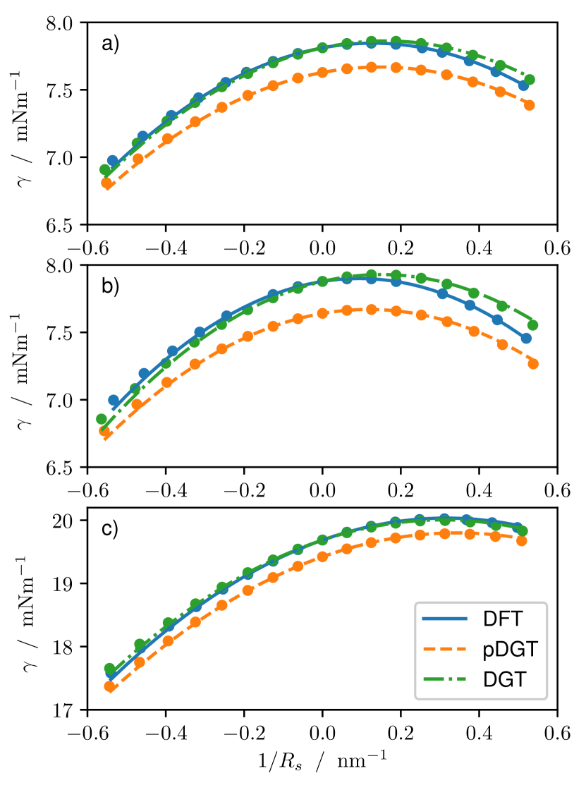
Figure 1: Comparison of the surface tension of droplets ($R_{s}>0$) and bubbles ($R_{s}<0$) (symbols) with the Helfrich expansion (lines) for pDGT, DFT and DGT. The influence parameter in DGT is found by fixing the value of the planar surface tension to the corresponding result from DFT. a) methane at $T=140\,\text{K}$ b) n-hexane at $T=400\,\text{K}$, c) water at $T=550\,\text{K}$

In Fig. 1, results from this comparison are shown for three different components and temperatures. In all cases, the surface tension of the droplets and bubbles is well approximated by the Helfrich expansion in the whole range of curvatures. In general, the different models also yield similar results, with the pDGT predicting slightly lower values for the surface tension for all curvatures. The planar surface tension from DGT is by construction equal to DFT. By increasing the curvature, the results start to differ with the effect being especially pronounced for n-hexane, the most elongated component considered.

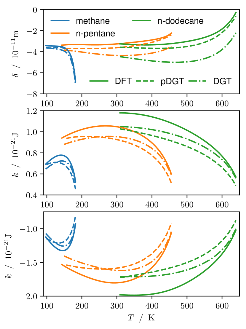
Figure 2: Tolman length and rigidities of n-alkanes. Comparison between DFT, pDGT and DGT predictions.

To obtain further insight about the chain length dependence of the Helfrich coefficients, we calculated them for n-alkanes of different lengths. Figure 2 presents the results for methane, n-pentane and n-dodecane. Two observations made in previous workRehner and Gross (2018a) can be confirmed here. The Tolman length of alkanes is over a wide temperature range very close to $-0.1$ times the segment diameter. In vicinity of the critical temperature however, the Tolman length deviates from this value. For small alkanes, the Tolman length decreases, whereas for longer alkanes the Tolman length increases. For methane, the different theories give similar results for the Tolman length. This conformity deteriorates for longer chains, with the magnitude of the DGT results being up to $50\,\%$ larger than the DFT results for n-dodecane.

A similar trend can be observed for the rigidity constants. The qualitative behavior is similar for all of the theories, but for longer chain lengths the difference between them increases. While the Tolman lengths from pDGT are close to the DFT results, both gradient based methods display comparable deviations from DFT for the rigidities, being up to $15\,\%$ for n-dodecane. Because bulk properties are described by the same equation of state for all considered theories, it is likely a difference in the description of structural properties that leads to the difference in predicted Helfrich coefficients. However, the way the different PCP-SAFT contributions affect the surface tension and the Helfrich coefficients is convoluted and not a simple linear combination. Hence, the role of the chain contribution in the different theories is not easily isolated. A more thorough investigation into the structure of interfaces of chain molecules, e.g. by molecular simulation, is advised to gain further insight about structural anisotropies at the interface.

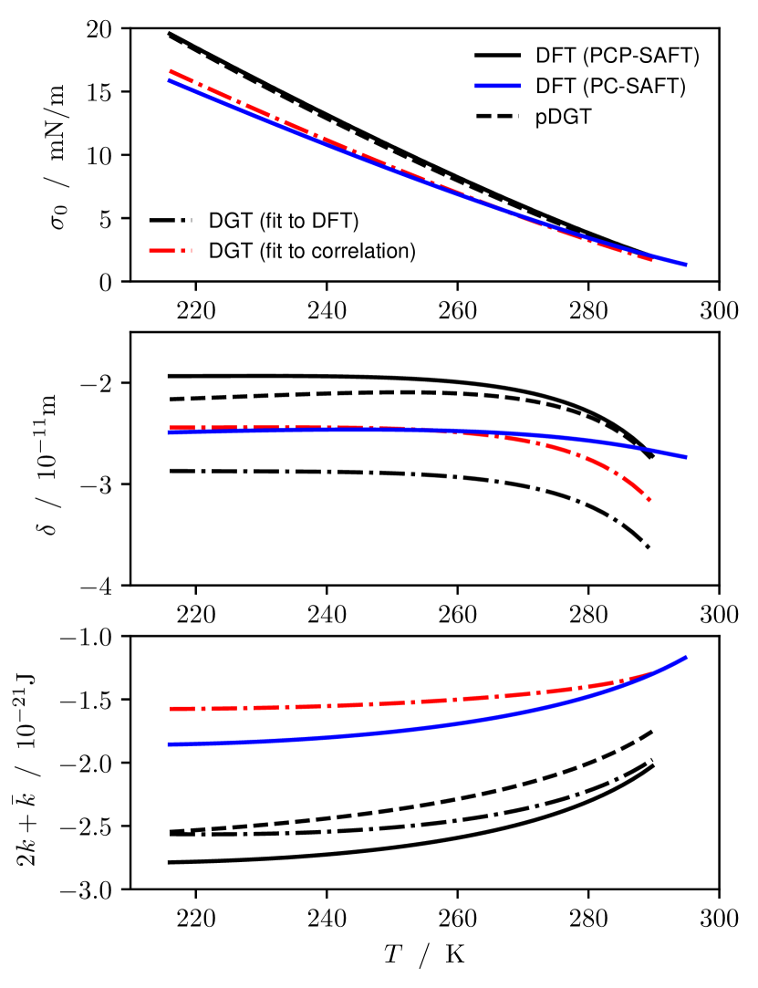
Figure 3: Tolman length and spherical rigidity of CO₂. Comparison between DFT, pDGT and DGT predictions. Except for the blue line all results are obtained using the PCP-SAFT equation of state. For DGT, the results are obtained by fitting to the surface tension from DFT (black) and to an empirical correlation Mulero, Cachadiña, and Parra (2012) (red).

To expand the study to polar components, the Helfrich coefficients of CO₂ are presented in Fig. 3. For homogeneous nucleation, the primary application of this framework, only spherical droplets are relevant. We find that the behavior of the two rigidities is very similar for all studied components. Therefore, from here on we only show the spherical rigidity $k_{s}=2k+\bar{k}$, which appears as the second order coefficient in a curvature expansion of the surface tension for a spherical geometry. The quantitative behavior of the different theories are similar for CO₂ and the alkanes. The predictions of the Tolman length from pDGT lie slightly below the DFT results with the difference decreasing with temperature. The DGT results on the other hand are significantly lower. For the rigidities, both pDGT and DGT predict larger values than DFT. We find that these are general trends for non-associating fluids, where results for other substances such as nitrogen and argon are included in the supplementary material.

Fig. 3-top shows that PC-SAFT predicts the surface tension of CO₂ to a reasonable accuracy, since DFT with PC-SAFT (blue solid line) agrees well with DGT for which the influence parameter was fitted to an empirical correlation Mulero, Cachadiña, and Parra (2012) for the surface tension (red dash-dot line). The surface tension from PCP-SAFT, however, lies above the experimental values. The values for the Tolman length and rigidities reflect this, where the Tolman length and rigidities from PC-SAFT and PCP-SAFT are significantly different. The prediction of the surface tension with the PC-SAFT equation of state is better than with PCP-SAFT, despite the latter describing the phase equilibrium and the critical point of CO₂ more accurately Gross and Vrabec (2006). The same trend can be seen for DGT, where there is a large difference between the Helfrich coefficients when the influence parameter has been fitted to DFT values (black dash-dot line) and an empirical correlation (red dash-dot line). This effect is especially pronounced for the rigidity, which decreases about $40\,\%$ in magnitude by fitting to the empirical surface tension rather than to DFT. Hence, an important basis for reliable estimates of the curvature dependence of the surface tension is accurate prediction of the planar surface tension.

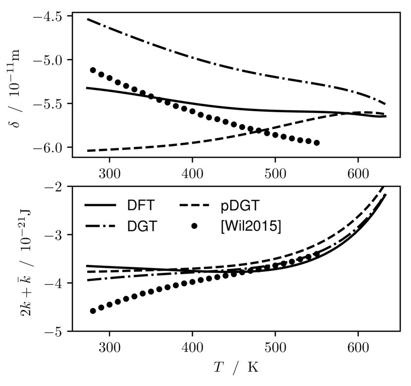
Figure 4: Tolman length and spherical rigidity of water. Comparison between DFT, pDGT and DGT predictions for the PCP-SAFT equation of state, as well as DGT results using CPA from previous workWilhelmsen, Bedeaux, and Reguera (2015a).

We next discuss the Helfrich coefficients for water, as this has been a popular example in the literature Wilhelmsen, Bedeaux, and Reguera (2015a); Menzl et al. (2016); Joswiak et al. (2016); Kim et al. (2018); Leong and Wang (2018). Since the numerous PCP-SAFT water parameter sets that have been published predict vastly different planar surface tensionsMairhofer and Gross (2018), new parameters have been obtained that use quasi experimental surface tension dataLemmon, McLinden, and Friend as additional input in the estimation. These parameters are for the 2B association schemeHuang and Radosz (1990) and include a fitted dipole moment. They are shown in Tab. 1.

$m$	.99214	$\mu$	1.6152 D
$\sigma$	3.0177 Å	$\kappa^{A_{i}B_{i}}$	.091799
$\varepsilon/k_{B}$	166.66 K	$\varepsilon^{A_{i}B_{i}}/k_{B}$	2685.1 K

Table 1: PCP-SAFT parameters for the 2B water model used in this work.

For the Tolman length, we find the same behavior for pDGT and DFT as for non-associating fluids. The Tolman length obtained from DGT however, is larger than the DFT result. The spherical rigidity shows a remarkable resemblance for the three different approaches. We further compare the spherical rigidity to previous resultsWilhelmsen, Bedeaux, and Reguera (2015a) that were calculated using DGT combined with the cubic plus association (CPA) Kontogeorgis et al. (1996) equation of state. The Tolman length has a comparable magnitude and the temperature dependence is the same for DGT with PCP-SAFT. For the rigidity at higher temperatures, we again observe good agreement. For lower temperatures, the results deviate by up to $25\,\%$. Since the influence parameters do not differ significantly between the different approaches, this deviation can be attributed to the difference in equation of state. Hence, the equation of state has an important role in the prediction of the Helfrich coefficients.

In conclusion, we find that the different descriptions of the considered Helmholtz energy functionals give relatively similar results. However, for strongly polar or elongated molecules, deviations between DFT and DGT should be expected, in particular for the Tolman length. Prerequisites for accurate prediction of the Helfrich coefficients are: a bulk equation of state that is able to describe the phase equilibrium well and a Helmholtz energy functional that is able to reproduce the planar surface tension accurately. As shown in the supplementary material, for alcohols, that are frequently used in nucleation experiments, the surface tension predictions using DFT and PCP-SAFT deviate significantly from experimental data. Therefore, further work has to be done to improve the parametrization of these components, before the influence of the curvature corrections on nucleation rates can be studied rigorously.

III.2 Mixtures

In a previous workAasen, Blokhuis, and Wilhelmsen (2018), it was shown that the values of the Helfrich coefficients for mixtures are significantly influenced by the choice of path through the metastable region. We emphasize that already for pure components, a deliberate choice has been made by choosing the isothermal path. An isentropic path is another possible choice.

The value of the surface tension of a droplet is only a function of the thermodynamic state and the choice of dividing surface, and does not depend on the path. A different path, however, leads to a different quality of the prediction using the Helfrich expansion and a different composition dependence of the coefficients. Following the recommendations in a previous study by Aasen et al.Aasen, Blokhuis, and Wilhelmsen (2018), we choose a straight path through the metastable region that keeps the liquid composition constant to first order.

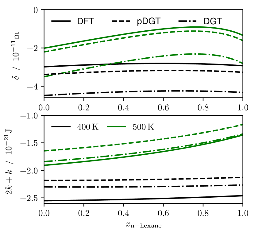
Figure 5: Composition dependence of the Tolman length and spherical rigidity for the binary mixture of n-hexane and n-heptane at different temperatures. Comparison between DFT, pDGT and DGT results.

We first study the behavior of a close to ideal mixture. To that end, we examine the n-hexane/n-heptane mixture at different temperatures with the binary interaction parameter $k_{ij}$ equal to 0. In Fig. 5, the Tolman length and the spherical rigidity are displayed as functions of the liquid mole fraction of n-hexane in the system. At lower temperatures, the pure component values of both coefficients are similar and there is almost no composition dependence. For temperatures close to the critical point, however, the Tolman length displays a non-linear dependence on the composition. The spherical rigidity is higher for n-hexane than for n-heptane closer to the critical point, but the composition dependence is still close to linear. Comparing the different theories, an almost constant deifference in predicted values can be observed over the whole composition range for both temperatures. Therefore, if a good agreement is obtained for the pure components, it can be expected that DGT using the geometric combining rule will also predict similar values as DFT and pDGT for this mixture.

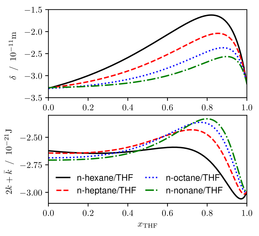
Figure 6: DFT result for the composition dependence of the Tolman length and spherical rigidity for the binary mixture of various n-alkanes with the polar component tetrahydrofuran (THF) at $298.15\,\text{K}$.

We extend the study to the more non ideal binary mixtures of n-alkanes with the polar solvent tetrahydrofuran (THF). Parameters for this system, including the binary interaction parameter $k_{ij}$ were obtained by Klink and GrossKlink and Gross (2014) and the DFT results using them were shown to concur well with experimental dataSauer and Gross (2017). In Fig. 6, the Tolman length and spherical rigidity are shown for the binary mixture of THF with n-hexane, n-heptane, n-octane and n-nonane at $T=298.15\,\mathrm{K}$. Although all of the pure components have almost the same Tolman length at this temperature, the Tolman lengths of the mixtures are significantly different, with a peak near $x_{\text{THF}}=0.8$. This effect is most pronounced at higher concentrations of THF and for smaller alkanes, with the Tolman length of the n-hexane/THF mixture being up to $50\,\%$ higher than both pure component values. Contrary to that, the spherical rigidity of the same system is constant in a large composition range until the value drops towards the pure component value of THF. For longer alkanes, a peak in the spherical rigidity is observed, similar to the Tolman length. A comparison to the gradient theories can be seen in the supplementary material. Also for the non-ideal mixtures, DGT predicts a similar composition dependence as DFT for the Helfrich coefficients, with the main difference being a nearly constant difference in predicted values, which is determined by the deviation between the pure component values.

IV Conclusion

The curvature dependence of the surface tension can be described by the Helfrich expansion, where the first and second order expansion coefficients are called the Tolman length and the rigidities. They are also referred to as the Helfrich coefficients.

In this work, we have derived general expressions that can be used for calculating Helfrich coefficients from any non-local Helmholtz energy functional based on weighted densities. The curvature expansion can be used to calculate the surface energy of arbitrarily shaped interfaces for pure component and mixtures.

We used the framework to compare predictions from non-local density functional theory (DFT) with results from density gradient theory (DGT) and predictive density gradient theory (pDGT). Good agreement between the different theories was observed for small, approximately spherical molecules. An increase in chain length led to larger differences in the predictions. We found that the values of the Helfrich coefficients are sensitive to the choice of influence parameter in DGT and to the prediction of the surface tension in DFT and pDGT. We showed that if a model is used that gives a good description of the phase equilibrium (including liquid densities) and the surface tension, good agreement can be expected between the different functional theories. However, the Helfrich coefficients also displayed a dependence on the equation of state.

For non ideal mixtures, the composition dependence of the Helfrich coefficients was found to be nonlinear. All three functionals studied gave very similar composition dependencies for the Helfrich coefficients, where the difference comes mainly from different predictions of the pure component values.

Further work is needed to describe the Helfrich coefficients of alcohols, since PC-SAFT and PCP-SAFT are currently unable to accurately predict their surface tensions. Because alcohols are frequently used in nucleation experiments, their Helfrich coefficients are of much interest.

supplementary material

See supplementary material for additional results for Helfrich coefficients, the derivation of the curvature expansion of convolution integrals and the simplification of the second order coefficient for DFT.

Appendix A Curvature expansion of convolution integrals

In non-local DFT using weighted densities, the density profile and the partial derivatives of the Helmholtz energy density are convolved with a weight function $\omega$. To reduce the amount of different symbols, we use the same symbol for the different representations of $\omega$ and use the independent variable as an indicator for which representation to use. The different representations are the weight function in real space $\omega(\mathbf{r})=\omega(r)$, the projection on the $z$-axis

$$\omega(z)=2\pi\int\limits_{|z|}^{\infty}\omega(r)r\mathrm{d}r$$ (65)

and the Fourier transform

$$\omega(k)=\int\limits_{-\infty}^{\infty}\omega(z)e^{-2\pi ikz}\mathrm{d}z=\int\limits_{0}^{\infty}\omega(r)\frac{2r}{k}\sin(2\pi kr)\mathrm{d}r.$$ (66)

The convolution of a spherically symmetric function $f(r)$ and a scalar weight function $\omega(r)$ can be expressed asRoth (2010)

$$f\stackrel{{\scriptstyle 3D}}{{\otimes}}\omega =\frac{1}{r}\int f(r-z^{\prime})(r-z^{\prime})\omega(z^{\prime})\mathrm{d}z^{\prime}$$

$$=f\otimes\omega-\frac{1}{r}f\otimes\left(z\omega\right)$$

$$=f\otimes\omega-f\otimes\left(z\omega\right)\frac{1}{R}+z\left(f\otimes\left(z\omega\right)\right)\frac{1}{R^{2}}+\ldots$$ (67)

The convolution of a cylindrically symmetric function with a scalar weight function is more intricate. The projection-slice theorem of the Fourier transform states, that the 3D Fourier transform can be replaced by a projection on one of the axes followed by the one-dimensional Fourier transform along the given axis. In a cylindrical geometry, the projection is known as the Abel transform. To our knowledge, no concise expression is available like in the spherical case. However, the curvature coefficients can still be derived by performing the curvature expansion on the general convolution integral itself. The expression we obtain is

$$f\stackrel{{\scriptstyle 3D}}{{\otimes}}\omega=f\otimes\omega-\frac{1}{2}f\otimes\left(z\omega\right)\frac{1}{R}\\ +\left(\frac{1}{2}z\left(f\otimes\left(z\omega\right)\right)-\frac{1}{8}f\otimes\tilde{\omega}\right)\frac{1}{R^{2}}+\ldots$$ (68)

The full derivation is shown in the supplementary material. The weight function, $\tilde{\omega}$ appearing in the last convolution is

$$\tilde{\omega}=z^{2}\omega-\int\limits_{z}^{\infty}\omega(z^{\prime})z^{\prime}\mathrm{d}z^{\prime}=z^{2}\omega-\left(z\omega\right)\otimes\Theta(-z)$$ (69)

with the Heaviside step function $\Theta(z)$. The two geometries can be combined in a general expression involving the geometry factor $g$, as

$$f\stackrel{{\scriptstyle 3D}}{{\otimes}}\omega=f\otimes\omega-\frac{g}{2}f\otimes\left(z\omega\right)\frac{1}{R}\\ +\left(\frac{g}{2}z\left(f\otimes\left(z\omega\right)\right)+\frac{g(g-2)}{8}f\otimes\tilde{\omega}\right)\frac{1}{R^{2}}+\ldots$$ (70)

Appendix B Convolutions in Fourier space

Aside from the convergence speed of the solver, the computation time of DFT is limited by the evaluation of the numerous convolution integrals. The calculation can be sped up using the convolution theorem of the Fourier transform. It states that the Fourier transform of a convolution is equal to the product of the Fourier transform of the functions that are being convolved. The Fourier transform of the density profiles and the partial derivatives can be calculated in $\mathcal{O}(N\log N)$ using the fast Fourier transform. The Fourier transform of the weight functions can be obtained analytically from Eq. (66). The other weight functions needed to calculate the Helfrich coefficients can be obtained from the derivatives of the weight functions in Fourier space, as

$$\mathcal{F}(z\omega) =\frac{i}{2\pi}\omega^{\prime}(k)~{}~{}~{}~{}~{}~{}\text{and}$$ (71)

$$\mathcal{F}(\tilde{\omega}) =\mathcal{F}\left(z^{2}\omega\right)-\mathcal{F}\left(z\omega\right)\mathcal{F}(\Theta(-z))$$

$$=-\frac{1}{4\pi^{2}}\omega^{\prime\prime}(k)-\frac{i}{2\pi}\omega^{\prime}(k)\left(\frac{1}{2}\delta(k)+\frac{i}{2\pi k}\right)$$

$$=\frac{1}{4\pi^{2}}\left(\frac{\omega^{\prime}(k)}{k}-\omega^{\prime\prime}(k)\right).$$ (72)

We focus on spherically symmetric weight functions, $\omega(r)$, $\omega(z)$ and $\omega(k)$ that are all even functions by construction. Therefore, $\omega^{\prime}(k=0)=0$ and the term involving the dirac distribution $\delta(k)$ cancels. Further, using L’Hôpital’s rule we find that $\mathcal{F}(\tilde{\omega})(k=0)=0$.

Appendix C Hyper-dual numbers

With the only exception being the derivative $\bm{c}_{\bm{\rho}0}$, all properties in the framework we discuss are related to at most second order partial derivatives of the Helmholtz energy density. Hyper-dual numbersFike and Alonso (2011) can be used to calculate the exact second partial derivatives and thus all related properties. The approach has recently been used in the context of equations of stateDiewald et al. (2018). Here, we propose its use to calculate the first and second partial derivatives of the non-local Helmholtz energy density in DFT and to calculate the different weight functions in Fourier space needed to calculate all convolution integrals for the curvature expansion. Therefore, the only properties that need to be implemented are the Helmholtz energy functional and the weight functions. All other properties, including derivatives of the underlying equation of state and the weight constants in pDGT are available through the hyper-dual numbers, making it simpler and less error-prone to include new functionals. This improvement in usability comes with increased computation time, since every operator and intrinsic function has to be evaluated for hyper-dual numbers. In particular for functions of many variables, there is significant redundancy when calculating derivatives. Therefore, in cases with many variables and simple derivatives like the FMT and chain functionals, it is advisable to override the hyper-dual differentiation with analytic derivatives to speed up the computation.

Appendix D Vector weighted densities

Some FMTRosenfeld (1989); Roth et al. (2002); Yu and Wu (2002a) and association functionalsYu and Wu (2002b) use vector weighted densities. To include those in the framework presented in this work, the expressions have to be amended accordingly. As we are still only considering spherically symmetric weight functions, we can write vector weight functions as $\vec{\omega}(\mathbf{r})=\omega_{r}(r)\vec{e}_{r}$ with the radial unit vector $\vec{e}_{r}$. The projection on the $z$-axis then becomes

$$\vec{\omega}(z)=\omega_{z}(z)\vec{e}_{z}=2\pi z\vec{e}_{z}\int\limits_{|z|}^{\infty}\omega_{r}(r)\mathrm{d}r$$ (73)

and the representation in Fourier space is

$$\vec{\omega}(\mathbf{k}) =\omega_{k}(k)\vec{e}_{k}=\vec{e}_{k}\int\limits_{-\infty}^{\infty}\omega_{z}(z)e^{-2\pi ikz}\mathrm{d}z$$

$$=\vec{e}_{k}\int\limits_{0}^{\infty}\omega_{r}(r)\frac{i}{\pi k^{2}}\left(2\pi kr\cos(2\pi kr)-\sin(2\pi kr)\right)\mathrm{d}r.$$ (74)

The convolution integrals involving vector weight functions are different from scalar weight functions. A detailed derivation of the handling of these convolutions is given in the supporting material. To include vector weighted densities in the framework presented in this work, the convolution integrals in Sec. II.2 have to be changed according to Tab. 2 for every vector weight function. The newly introduced weight function $\hat{\bm{\omega}}_{\alpha z}$ is defined as

$$\hat{\bm{\omega}}_{\alpha z}=\int\limits_{z}^{\infty}\bm{\omega}_{\alpha z}(z^{\prime})\mathrm{d}z^{\prime}$$ (75)

and all combinations of weight functions are again easily obtained in Fourier space as

$$\mathcal{F}(z\omega_{z}\pm\hat{\omega}_{z}) =\frac{i}{2\pi}\left(\omega_{k}^{\prime}(k)\pm\frac{\omega_{k}(k)}{k}\right)$$ (76)

$$\mathcal{F}(z^{2}\omega_{z}\pm z\hat{\omega}_{z}) =\frac{-1}{4\pi^{2}}\left(\omega_{k}^{\prime\prime}(k)\pm\left(\frac{\omega_{k}^{\prime}(k)}{k}-\frac{\omega_{k}(k)}{k^{2}}\right)\right).$$ (77)

scalar expression	vector expression	equations
$\bm{\rho}_{0|1}\otimes\bm{\omega}_{\alpha}$	$\bm{\rho}_{0|1}\otimes\bm{\omega}_{\alpha z}$	(37), (38)
$f_{\alpha 0|1}\otimes\bm{\omega}_{\alpha}$	$-f_{\alpha 0|1}\otimes\bm{\omega}_{\alpha z}$	(42), (43)
$\bm{\rho}_{0}\otimes\left(z\bm{\omega}_{\alpha}\right)$	$\bm{\rho}_{0}\otimes\left(z\bm{\omega}_{\alpha z}-\hat{\bm{\omega}}_{\alpha z}\right)$	(44) - (46), (38)
$f_{\alpha 0}\otimes\left(z\bm{\omega}_{\alpha}\right)$	$-f_{\alpha 0}\otimes\left(z\bm{\omega}_{\alpha z}+\hat{\bm{\omega}}_{\alpha z}\right)$	(45), (43)
$\bm{\rho}_{0}\otimes\tilde{\bm{\omega}}_{\alpha}$	$\bm{\rho}_{0}\otimes\left(z^{2}\bm{\omega}_{\alpha z}+z\hat{\bm{\omega}}_{\alpha z}\right)$	(45)
$\bm{\rho}_{0}\otimes\tilde{\bm{\omega}}_{\alpha}$	$\bm{\rho}_{0}\otimes\left(z^{2}\bm{\omega}_{\alpha z}-z\hat{\bm{\omega}}_{\alpha z}\right)$	(46)

Table 2: Replacement for convolution integrals for vector weighted densities.

References

- Iland et al. (2007) K. Iland, J. Wölk, R. Strey, and D. Kashchiev, “Argon Nucleation in a Cryogenic Pulse Chamber,” Journal of Chemical Physics 127, 154506 (2007).
- Vehkamäki (2006) H. Vehkamäki, Classical nucleation theory in multicomponent systems (Springer Science & Business Media, 2006).
- ten Wolde and Frenkel (1998) P. R. ten Wolde and D. Frenkel, “Computer simulation study of gas-liquid nucleation in a Lennard-Jones system,” The Journal of Chemical Physics 109, 9901 (1998).
- Wilhelmsen, Bedeaux, and Reguera (2015a) Ø. Wilhelmsen, D. Bedeaux, and D. Reguera, “Communication: Tolman length and rigidity constants of water and their role in nucleation,” The Journal of Chemical Physics 142, 171103 (2015a).
- Nguyen et al. (2018) V. D. Nguyen, F. C. Schoemaker, E. M. Blokhuis, and P. Schall, “Measurement of the Curvature-Dependent Surface Tension in Nucleating Colloidal Liquids,” Physical Review Letters 121, 246102 (2018).
- Helfrich (1973) W. Helfrich, “Elastic properties of lipid bilayers: Theory and possible experiments,” Zeitschrift für Naturforschung C 28 (1973), 10.1515/znc-1973-11-1209.
- Kim et al. (2018) S. Kim, D. Kim, J. Kim, S. An, and W. Jhe, “Direct evidence for curvature-dependent surface tension in capillary condensation: Kelvin equation at molecular scale,” Physical Review X 8 (2018), 10.1103/PhysRevX.8.041046.
- Tolman (1949) R. C. Tolman, “The effect of droplet size on surface tension,” The Journal of Chemical Physics 17, 333–337 (1949).
- Wilhelmsen, Bedeaux, and Reguera (2015b) Ø. Wilhelmsen, D. Bedeaux, and D. Reguera, “Tolman length and rigidity constants of the lennard-jones fluid,” The Journal of Chemical Physics 142, 064706 (2015b).
- Bruot and Caupin (2016) N. Bruot and F. Caupin, “Curvature dependence of the liquid-vapor surface tension beyond the tolman approximation,” Physical Review Letters 116, 056102 (2016).
- Aasen, Blokhuis, and Wilhelmsen (2018) A. Aasen, E. M. Blokhuis, and . Wilhelmsen, “Tolman lengths and rigidity constants of multicomponent fluids: Fundamental theory and numerical examples,” The Journal of Chemical Physics 148, 204702 (2018).
- Rehner and Gross (2018a) P. Rehner and J. Gross, “Surface tension of droplets and tolman lengths of real substances and mixtures from density functional theory,” The Journal of Chemical Physics 148, 164703 (2018a).
- Blokhuis and Kuipers (2006) E. M. Blokhuis and J. Kuipers, “Thermodynamic expressions for the tolman length,” Journal of Chemical Physics 124, 74701–74701 (2006).
- Li and Wu (2007) Z. Li and J. Wu, “Toward a quantitative theory of ultrasmall liquid droplets and vapor liquid nucleation,” Industrial & Engineering Chemistry Research 47, 4988–4995 (2007).
- Block et al. (2010) B. J. Block, S. K. Das, M. Oettel, P. Virnau, and K. Binder, “Curvature dependence of surface free energy of liquid drops and bubbles: A simulation study,” The Journal of Chemical Physics 133, 154702 (2010).
- Tröster et al. (2012) A. Tröster, M. Oettel, B. Block, P. Virnau, and K. Binder, “Numerical approaches to determine the interface tension of curved interfaces from free energy calculations,” The Journal of Chemical Physics 136, 064709 (2012).
- van Giessen and Blokhuis (2002) A. E. van Giessen and E. M. Blokhuis, “Determination of curvature corrections to the surface tension of a liquid–vapor interface through molecular dynamics simulations,” The Journal of Chemical Physics 116, 302–310 (2002).
- Lei et al. (2005) Y. A. Lei, T. Bykov, S. Yoo, and X. C. Zeng, “The Tolman Length: Is it Positive or Negative?” J. Am. Chem. Soc. 127, 15346 (2005).
- Horsch et al. (2012) M. Horsch, H. Hasse, A. K. Shchekin, A. Agarwal, S. Eckelsbach, J. Vrabec, E. A. Müller, and G. Jackson, “Excess equimolar radius of liquid drops,” Physical Review E 85, 031605 (2012).
- van Giessen and Blokhuis (2009) A. E. van Giessen and E. M. Blokhuis, “Direct determination of the tolman length from the bulk pressures of liquid drops via molecular dynamics simulations,” The Journal of Chemical Physics 131, 164705 (2009).
- Sampayo et al. (2010) J. G. Sampayo, A. Malijevský, E. A. Müller, E. de Miguel, and G. Jackson, “Communications: Evidence for the role of fluctuations in the thermodynamics of nanoscale drops and the implications in computations of the surface tension,” The Journal of Chemical Physics 132, 141101 (2010).
- Blokhuis and van Giessen (2013) E. M. Blokhuis and A. E. van Giessen, “Density functional theory of a curved liquid-vapour interface: evaluation of the rigidity constants,” Journal of Physics: Condensed Matter 25, 225003 (2013).
- Menzl et al. (2016) G. Menzl, M. A. Gonzalez, P. Geiger, F. Caupin, J. L. F. Abascal, C. Valeriani, and C. Dellago, “Molecular mechanism for cavitation in water under tension,” Proceedings of the National Academy of Sciences 113, 13582–13587 (2016).
- Joswiak et al. (2013) M. N. Joswiak, N. Duff, M. F. Doherty, and B. Peters, “Size-dependent surface free energy and tolman-corrected droplet nucleation of tip4p/2005 water,” The Journal of Physical Chemistry Letters 4, 4267–4272 (2013), pMID: 26296177.
- Joswiak et al. (2016) M. N. Joswiak, R. Do, M. F. Doherty, and B. Peters, “Energetic and entropic components of the tolman length for mw and tip4p/2005 water nanodroplets,” Journal of Chemical Physics 145, 204703 (2016).
- Kanduč (2017) M. Kanduč, “Going beyond the standard line tension: Size-dependent contact angles of water nanodroplets,” The Journal of Chemical Physics 147, 174701 (2017).
- Leong and Wang (2018) K.-Y. Leong and F. Wang, “A molecular dynamics investigation of the surface tension of water nanodroplets and a new technique for local pressure determination through density correlation,” The Journal of Chemical Physics 148, 144503 (2018).
- Fisher and Wortis (1984) M. P. A. Fisher and M. Wortis, “Curvature corrections to the surface tension of fluid drops: Landau theory and a scaling hypothesis,” Physical Review B 29, 6252–6260 (1984).
- Blokhuis and Bedeaux (1993) E. M. Blokhuis and D. Bedeaux, “Van der waals theory of curved surfaces,” Molecular Physics 80, 705–720 (1993).
- van Giessen, Blokhuis, and Bukman (1998) A. E. van Giessen, E. M. Blokhuis, and D. J. Bukman, “Mean field curvature corrections to the surface tension,” The Journal of Chemical Physics 108, 1148–1156 (1998).
- Barrett (2009) J. C. Barrett, “On the thermodynamic expansion of the nucleation free-energy barrier,” The Journal of Chemical Physics 131, 084711 (2009).
- Rehner and Gross (2018b) P. Rehner and J. Gross, “Predictive density gradient theory based on nonlocal density functional theory,” Physical Review E 98, 063312 (2018b).
- Koenig (1950) F. O. Koenig, “On the thermodynamic relation between surface tension and curvature,” The Journal of Chemical Physics 18, 449–459 (1950).
- Rosenfeld (1989) Y. Rosenfeld, “Free-energy model for the inhomogeneous hard-sphere fluid mixture and density-functional theory of freezing,” Physical Review Letters 63, 980–983 (1989).
- Tarazona (1985) P. Tarazona, “Free-energy density functional for hard spheres,” Physical Review A 31, 2672–2679 (1985).
- Mairhofer and Gross (2017a) J. Mairhofer and J. Gross, “Numerical aspects of classical density functional theory for one-dimensional vapor-liquid interfaces,” Fluid Phase Equilibria 444, 1–12 (2017a).
- Anderson (1965) D. G. Anderson, “Iterative procedures for nonlinear integral equations,” Journal of the ACM 12, 547–560 (1965).
- Miqueu et al. (2004) C. Miqueu, B. Mendiboure, C. Graciaa, and J. Lachaise, “Modelling of the surface tension of binary and ternary mixtures with the gradient theory of fluid interfaces,” Fluid Phase Equilibria 218, 189 – 203 (2004).
- Miqueu et al. (2005) C. Miqueu, B. Mendiboure, A. Graciaa, and J. Lachaise, “Modeling of the surface tension of multicomponent mixtures with the gradient theory of fluid interfaces,” Industrial & Engineering Chemistry Research 44, 3321–3329 (2005).
- Mairhofer and Gross (2017b) J. Mairhofer and J. Gross, “Modeling of interfacial properties of multicomponent systems using density gradient theory and pcp-saft,” Fluid Phase Equilibria 439, 31–42 (2017b).
- Kou, Sun, and Wang (2015) J. Kou, S. Sun, and X. Wang, “Efficient numerical methods for simulating surface tension of multi-component mixtures with the gradient theory of fluid interfaces,” Computer Methods in Applied Mechanics and Engineering 292, 92 – 106 (2015), special Issue on Advances in Simulations of Subsurface Flow and Transport (Honoring Professor Mary F. Wheeler).
- Liang, Michelsen, and Kontogeorgis (2016) X. Liang, M. L. Michelsen, and G. M. Kontogeorgis, “A density gradient theory based method for surface tension calculations,” Fluid Phase Equilibria 428, 153 – 163 (2016), theo W. de Loos Festschrift.
- Gross and Sadowski (2001) J. Gross and G. Sadowski, “Perturbed-chain saft: An equation of state based on a perturbation theory for chain molecules,” Industrial & Engineering Chemistry Research 40, 1244–1260 (2001).
- Gross (2005) J. Gross, “An equation-of-state contribution for polar components: Quadrupolar molecules,” AIChE Journal 51, 2556–2568 (2005).
- Gross and Vrabec (2006) J. Gross and J. Vrabec, “An equation-of-state contribution for polar components: Dipolar molecules,” AIChE Journal 52, 1194–1204 (2006).
- Roth (2010) R. Roth, “Fundamental measure theory for hard-sphere mixtures: a review,” Journal of Physics: Condensed Matter 22, 063102 (2010).
- Roth et al. (2002) R. Roth, R. Evans, A. Lang, and G. Kahl, “Fundamental measure theory for hard-sphere mixtures revisited: the white bear version,” Journal of Physics: Condensed Matter 14, 12063 (2002).
- Yu and Wu (2002a) Y.-X. Yu and J. Wu, “Structures of hard-sphere fluids from a modified fundamental-measure theory,” The Journal of Chemical Physics 117, 10156–10164 (2002a).
- Kierlik and Rosinberg (1990) E. Kierlik and M. L. Rosinberg, “Free-energy density functional for the inhomogeneous hard-sphere fluid: Application to interfacial adsorption,” Physical Review A 42, 3382–3387 (1990).
- Boublík (1970) T. Boublík, “Hard-sphere equation of state,” The Journal of Chemical Physics 53, 471–472 (1970).
- Mansoori et al. (1971) G. A. Mansoori, N. F. Carnahan, K. E. Starling, and T. W. Leland, “Equilibrium thermodynamic properties of the mixture of hard spheres,” The Journal of Chemical Physics 54, 1523–1525 (1971).
- Carnahan and Starling (1969) N. F. Carnahan and K. E. Starling, “Equation of state for nonattracting rigid spheres,” The Journal of Chemical Physics 51, 635–636 (1969).
- Tripathi and Chapman (2005a) S. Tripathi and W. G. Chapman, “Microstructure of inhomogeneous polyatomic mixtures from a density functional formalism for atomic mixtures,” The Journal of Chemical Physics 122, 094506 (2005a).
- Tripathi and Chapman (2005b) S. Tripathi and W. G. Chapman, “Microstructure and thermodynamics of inhomogeneous polymer blends and solutions,” Physical Review Letters 94, 087801 (2005b).
- Yu and Wu (2002b) Y.-X. Yu and J. Wu, “A fundamental-measure theory for inhomogeneous associating fluids,” The Journal of Chemical Physics 116, 7094–7103 (2002b).
- Sauer and Gross (2017) E. Sauer and J. Gross, “Classical density functional theory for liquid–fluid interfaces and confined systems: A functional for the perturbed-chain polar statistical associating fluid theory equation of state,” Industrial & Engineering Chemistry Research 56, 4119–4135 (2017).
- Sauer et al. (2018) E. Sauer, A. Terzis, M. Theiss, B. Weigand, and J. Gross, “Prediction of contact angles and density profiles of sessile droplets using classical density functional theory based on the pcp-saft equation of state,” Langmuir 34, 12519–12531 (2018), pMID: 30247038.
- Sauer and Gross (2019) E. Sauer and J. Gross, “Prediction of adsorption isotherms and selectivities: Comparison between classical density functional theory based on the perturbed-chain statistical associating fluid theory equation of state and ideal adsorbed solution theory,” Langmuir 35, 11690–11701 (2019), pMID: 31403314.
- Klink and Gross (2014) C. Klink and J. Gross, “A density functional theory for vapor-liquid interfaces of mixtures using the perturbed-chain polar statistical associating fluid theory equation of state,” Industrial & Engineering Chemistry Research 53, 6169–6178 (2014).
- Mulero, Cachadiña, and Parra (2012) A. Mulero, I. Cachadiña, and M. I. Parra, “Recommended correlations for the surface tension of common fluids,” Journal of Physical and Chemical Reference Data 41, 043105 (2012).
- Mairhofer and Gross (2018) J. Mairhofer and J. Gross, “Modeling properties of the one-dimensional vapor-liquid interface: Application of classical density functional and density gradient theory,” Fluid Phase Equilibria 458, 243 – 252 (2018).
- (62) E. W. Lemmon, M. O. McLinden, and D. G. Friend, “Nist chemistry webbook, nist standard reference database number 69,” (National Institute of Standards and Technology, Gaithersburg MD, 20899) Chap. Thermophysical Properties of Fluid Systems, , http://webbook.nist.gov, (retrieved July 15, 2016).
- Huang and Radosz (1990) S. H. Huang and M. Radosz, “Equation of state for small, large, polydisperse, and associating molecules,” Industrial & Engineering Chemistry Research 29, 2284–2294 (1990).
- Kontogeorgis et al. (1996) G. M. Kontogeorgis, E. C. Voutsas, I. V. Yakoumis, and D. P. Tassios, “An equation of state for associating fluids,” Industrial & Engineering Chemistry Research 35, 4310–4318 (1996).
- Fike and Alonso (2011) J. Fike and J. Alonso, “The development of hyper-dual numbers for exact second-derivative calculations,” in 49th AIAA Aerospace Sciences Meeting including the New Horizons Forum and Aerospace Exposition (2011).
- Diewald et al. (2018) F. Diewald, M. Heier, M. Horsch, C. Kuhn, K. Langenbach, H. Hasse, and R. Müller, “Three-dimensional phase field modeling of inhomogeneous gas-liquid systems using the pets equation of state,” The Journal of Chemical Physics 149, 064701 (2018).