Learning Model Bias

Abstract

In this paper the problem of learning appropriate domain-specific bias is addressed. It is shown that this can be achieved by learning many related tasks from the same domain, and a theorem is given bounding the number tasks that must be learnt. A corollary of the theorem is that if the tasks are known to possess a common internal representation or preprocessing then the number of examples required per task for good generalisation when learning $n$ tasks simultaneously scales like $O(a+\frac{b}{n})$, where $O(a)$ is a bound on the minimum number of examples requred to learn a single task, and $O(a+b)$ is a bound on the number of examples required to learn each task independently. An experiment providing strong qualitative support for the theoretical results is reported.

1 Introduction

It has been argued (see [6]) that the main problem in machine learning is the biasing of a learner’s hypothesis space sufficiently well to ensure good generalisation from a small number of examples. Once suitable biases have been found the actual learning task is relatively trivial. Exisiting methods of bias generally require the input of a human expert in the form of heuristics, hints [1], domain knowledge, etc . Such methods are clearly limited by the accuracy and reliability of the expert’s knowledge and also by the extent to which that knowledge can be transferred to the learner. Here I attempt to solve some of these problems by introducing a method for automatically learning the bias.

The central idea is that in many learning problems the learner is typically embedded within an environment or domain of related learning tasks and that the bias appropriate for a single task is likely to be appropriate for other tasks within the same environment. A simple example is the problem of handwritten character recognition. A preprocessing stage that identifies and removes any (small) rotations, dilations and translations of an image of a character will be advantageous for recognising all characters. If the set of all individual character recognition problems is viewed as an environment of learning tasks, this preprocessor represents a bias that is appropriate to all tasks in the environment. It is likely that there are many other currently unknown biases that are also appropriate for this environment. We would like to be able to learn these automatically.

Bias that is appropriate for all tasks must be learnt by sampling from many tasks. If only a single task is learnt then the bias extracted is likely to be specific to that task. For example, if a network is constructed as in figure 1 and the output nodes are simultaneously trained on many similar problems, then the hidden layers are more likely to be useful in learning a novel problem of the same type than if only a single problem is learnt. In the rest of this paper I develop a general theory of bias learning based upon the idea of learning multiple related tasks. The theory shows that a learner’s generalisation performance can be greatly improved by learning related tasks and that if sufficiently many tasks are learnt the learner’s bias can be extracted and used to learn novel tasks.

Other authors that have empirically investigated the idea of learning multiple related tasks include [5] and [8].

2 Learning Bias

For the sake of argument I consider learning problems that amount to minimizing the mean squared error of a function $h$ over some training set $D$. A more general formulation based on statistical decision theory is given in [3]. Thus, it is assumed that the learner receives a training set of (possibly noisy) input-output pairs $D=\{(x_{1},y_{1}),\dots,(x_{m},y_{m})\}$, drawn according to a probability distribution $P$ on ${X\times Y}$ ($X$ being the input space and $Y$ being the output space) and searches through its hypothesis space ${\cal H}$ for a function $h\colon X\to Y$ minimizing the empirical error,

$${\hat{E}}(h,D)=\frac{1}{m}\sum_{i=1}^{m}(h(x_{i})-y_{i})^{2}.$$ (1)

The true error or generalisation error of $h$ is the expected error under $P$:

$$E(h,P)=\int_{{X\times Y}}(h(x)-y)^{2}\,dP(x,y).$$ (2)

The hope of course is that an $h$ with a small empirical error on a large enough training set will also have a small true error, i.e. it will generalise well.

I model the environment of the learner as a pair $({\cal P},Q)$ where ${\cal P}=\{P\}$ is a set of learning tasks and $Q$ is a probability measure on ${\cal P}$. The learner is now supplied not with a single hypothesis space ${\cal H}$ but with a hypothesis space family ${\mathbb{H}}=\{{\cal H}\}$. Each ${\cal H}\in{\mathbb{H}}$ represents a different bias the learner has about the environment. For example, one ${\cal H}$ may contain functions that are very smooth, whereas another ${\cal H}$ might contain more wiggly functions. Which hypothesis space is best will depend on the kinds of functions in the environment. To determine the best ${\cal H}\in{\mathbb{H}}$ for $({\cal P},Q)$, we provide the learner not with a single training set $D$ but with $n$ such training sets $D_{1},\dots,D_{n}$. Each $D_{i}$ is generated by first sampling from ${\cal P}$ according to $Q$ to give $P_{i}$ and then sampling $m$ times from ${X\times Y}$ according to $P_{i}$ to give $D_{i}=\{(x_{i1},y_{i1}),\dots,(x_{im},y_{im})\}$. The learner searches for the hypothesis space ${\cal H}\in{\mathbb{H}}$ with minimal empirical error on $D_{1},\dots,D_{n}$, where this is defined by

$${\hat{E}}^{*}({\cal H},D_{1},\dots,D_{n})=\frac{1}{n}\sum_{i=1}^{n}\inf_{h\in{\cal H}}{\hat{E}}(h,D_{i}).$$ (3)

The hypothesis space ${\cal H}$ with smallest empirical error is the one that is best able to learn the $n$ data sets on average.

There are two ways of measuring the true error of a bias learner. The first is how well it generalises on the $n$ tasks $P_{1},\dots,P_{n}$ used to generate the training sets. Assuming that in the process of minimising (3) the learner generates $n$ functions $h_{1},\dots,h_{n}\in{\cal H}$ with minimal empirical error on their respective training sets, the learner’s true error is measured by:

$$E^{n}(h_{1},\dots,h_{n},P_{1},\dots,P_{n})=\frac{1}{n}\sum_{i=1}^{n}E(h_{i},P_{i}).$$ (4)

Note that in this case the learner’s empirical error is given by ${\hat{E}}^{n}(h_{1},\dots,h_{n},D_{1},\dots,D_{n})=\frac{1}{n}\sum_{i=1}^{n}{\hat{E}}(h_{i},D_{i}).$ The second way of measuring the generalisation error of a bias learner is to determine how good ${\cal H}$ is for learning novel tasks drawn from the environment $({\cal P},Q)$:

$$E^{*}({\cal H},Q)=\int_{\cal P}\inf_{h\in{\cal H}}E(h,P)\,dQ(P)$$ (5)

A learner that has found an ${\cal H}$ with a small value of (5) can be said to have learnt to learn the tasks in ${\cal P}$ in general. To state the bounds ensuring these two types of generalisation a few more definitions must be introduced.

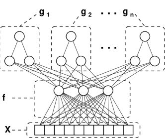
Figure 1: Net for learning multiple tasks. Input $x_{ij}$ from training set $D_{i}$ is propagated forwards through the internal representation $f$ and then only through the output network $g_{i}$. The error $\left[g_{i}(f(x_{ij}))-y_{ij}\right]^{2}$ is similarly backpropagated only through the output network $g_{i}$ and then $f$. Weight updates are performed after all training sets $D_{1},\dots,D_{n}$ have been presented.

Definition 1.

Let ${\mathbb{H}}=\{{\cal H}\}$ be a hypothesis space family. Let ${\mathbb{H}}_{\sigma}=\{h\in{\cal H}\colon{\cal H}\in{\mathbb{H}}\}$. For any $h\colon X\to Y$, define a map $h\colon{X\times Y}\to[0,1]$ by $h(x,y)=(h(x)-y)^{2}$. Note the abuse of notation: $h$ stands for two different functions depending on its argument. Given a sequence of $n$ functions ${\vec{h}}=(h_{1},\dots,h_{n})$ let ${\vec{h}}\colon({X\times Y})^{n}\to[0,1]$ be the function $(x_{1},y_{1},\dots,x_{n},y_{n})\mapsto\frac{1}{n}\sum_{i=1}^{n}h_{i}(x_{i},y_{i})$. Let ${\cal H}^{n}$ be the set of all such functions where the $h_{i}$ are all chosen from ${\cal H}$. Let ${\mathbb{H}}^{n}=\{{\cal H}^{n}\colon{\cal H}\in H\}$. For each ${\cal H}\in{\mathbb{H}}$ define ${\cal H}^{*}\colon{\cal P}\to[0,1]$ by ${\cal H}^{*}(P)=\inf_{h\in{\cal H}}E(h,P)$ and let ${\mathbb{H}}^{*}=\{{\cal H}^{*}\colon{\cal H}\in{\mathbb{H}}\}$.

Definition 2.

Given a set of functions ${\cal H}$ from any space $Z$ to $[0,1]$, and any probability measure on $Z$, define the pseudo-metric $d_{P}$ on ${\cal H}$ by

$$d_{P}(h,h^{\prime})=\int_{Z}|h(z)-h^{\prime}(z)|\,dP(z).$$

Denote the smallest ${\varepsilon}$-cover of $\left({\cal H},d_{P}\right)$ by ${\cal N}\left({\varepsilon},{\cal H},d_{P}\right)$. Define the ${\varepsilon}$-capacity of ${\cal H}$ by

$${\cal C}({\varepsilon},{\cal H})=\sup_{P}{\cal N}\left({\varepsilon},{\cal H},d_{P}\right)$$

where the supremum is over all discrete probability measures $P$ on $Z$.

Definition 2 will be used to define the ${\varepsilon}$-capacity of spaces such as ${\mathbb{H}}^{*}$ and ${\left[{\mathbb{H}}^{n}\right]_{\sigma}}$, where from definition 1 the latter is ${\left[{\mathbb{H}}^{n}\right]_{\sigma}}=\{{\vec{h}}\in{\cal H}^{n}\colon{\cal H}\in H\}$.

The following theorem bounds the number of tasks and examples per task required to ensure that the hypothesis space learnt by a bias learner will, with high probability, contain good solutions to novel tasks in the same environment.

Theorem 1.

Let the $n$ training sets $D_{1},\dots,D_{n}$ be generated by sampling $n$ times from the environment ${\cal P}$ according to $Q$ to give $P_{1},\dots,P_{n}$, and then sampling $m$ times from each $P_{i}$ to generate $D_{i}$. Let ${\mathbb{H}}=\{{\cal H}\}$ be a hypothesis space family and suppose a learner chooses $\hat{{\cal H}}\in{\mathbb{H}}$ minimizing (3) on $D_{1},\dots,D_{n}$. For all ${\varepsilon}>0$ and $0<\delta<1$, if

$$n = O\left(\frac{1}{{\varepsilon}^{2}}\ln\frac{{\cal C}\left({\varepsilon},{\mathbb{H}}^{*}\right)}{\delta}\right),$$

$$\text{and}\quad m = O\left(\frac{1}{n{\varepsilon}^{2}}\ln\frac{{\cal C}({\varepsilon},{\left[{\mathbb{H}}^{n}\right]_{\sigma}})}{\delta}\right)$$

then

$$\Pr\left\{D_{1},\dots,D_{n}\colon|{\hat{E}}^{*}(\hat{{\cal H}},D_{1},\dots,D_{n})-E^{*}(\hat{{\cal H}},Q)|>{\varepsilon}\right\}\leq\delta.$$

The bound on $m$ in theorem 1 is the also the number of examples required per task to ensure generalisation of the first kind mentioned above. That is, it is the number of examples required in each data set $D_{i}$ to ensure good generalisation on average across all $n$ tasks when using the hypothesis space family ${\mathbb{H}}$. If we let $m({\mathbb{H}},n,{\varepsilon},\delta)$ be the number of examples required per task to ensure that $\Pr\left\{D_{1},\dots,D_{n}\colon|{\hat{E}}^{n}(h_{1},\dots,h_{n},D_{1},\dots,D_{n})-E^{n}(h_{1},\dots,h_{n},P_{1},\dots,P_{n})|>{\varepsilon}\right\}\leq\delta$, where all $h_{i}\in{\cal H}$ for some fixed ${\cal H}\in{\mathbb{H}}$, then

$$G({\mathbb{H}},n,{\varepsilon},\delta)=\frac{m({\mathbb{H}},1,{\varepsilon},\delta)}{m({\mathbb{H}},n,{\varepsilon},\delta)}$$

represents the advantage in learning $n$ tasks as opposed to one task (the ordinary learning scenario). Call $G({\mathbb{H}},n,{\varepsilon},\delta)$ the $n$-task gain of ${\mathbb{H}}$. Using the fact [3] that

$${\cal C}\left({\varepsilon},{\mathbb{H}}_{\sigma}\right)\leq{\cal C}\left({\varepsilon},{\left[{\mathbb{H}}^{n}\right]_{\sigma}}\right)\leq{\cal C}\left({\varepsilon},{\mathbb{H}}_{\sigma}\right)^{n},$$

and the formula for $m$ from theorem 1, we have,

$$1\leq G({\mathbb{H}},n,{\varepsilon},\delta)\leq n.$$

Thus, at least in the worst case analysis here, learning $n$ tasks in the same environment can result in anything from no gain at all to an $n$-fold reduction in the number of examples required per task. In the next section a very intuitive analysis of the conditions leading to the extreme values of $G(H,n,{\varepsilon},\delta)$ is given for the situation where an internal representation is being learnt for the environment. I will also say more about the bound on the number of tasks ($n$) in theorem 1.

3 Learning Internal Representations with Neural Networks

In figure 1 $n$ tasks are being learnt using a common representation $f$. In this case ${\left[{\mathbb{H}}^{n}\right]_{\sigma}}$ is the set of all possible networks formed by choosing the weights in the representation and output networks. ${\mathbb{H}}_{\sigma}$ is the same space with a single output node. If the $n$ tasks were learnt independently (i.e. without a common representation) then each task would use its own copy of $H_{\sigma}$, i.e. we wouldn’t be forcing the tasks to all use the same representation.

Let $W_{R}$ be the total number of weights in the representation network and $W_{O}$ be the number of weights in an individual output network. Suppose also that all the nodes in each network are Lipschitz bounded. Then it can be shown [3] that $\ln{\cal C}\left({\varepsilon},{\left[{\mathbb{H}}^{n}\right]_{\sigma}}\right)=O\left(\left(W_{O}+\frac{W_{R}}{n}\right)\ln\frac{1}{{\varepsilon}}\right)$ and $\ln{\cal C}\left({\varepsilon},{\mathbb{H}}^{*}\right)=O\left(W_{R}\ln\frac{1}{{\varepsilon}}\right)$. Substituting these bounds into theorem 1 shows that to generalise well on average on $n$ tasks using a common representation requires $m=O\left(\frac{1}{{\varepsilon}^{2}}\left[\left(W_{O}+\frac{W_{R}}{n}\right)\ln\frac{1}{{\varepsilon}}+\frac{1}{n}\ln\frac{1}{\delta}\right]\right)=O\left(a+\frac{b}{n}\right)$ examples of each task. In addition, if $n=O\left(\frac{1}{{\varepsilon}^{2}}W_{R}\ln\frac{1}{{\varepsilon}}\right)$ then with high probability the resulting representation will be good for learning novel tasks from the same environment. Note that this bound is very large. However it results from a worst-case analysis and so is highly likely to be beaten in practice. This is certainly borne out by the experiment in the next section.

The learning gain $G(H,n,{\varepsilon})$ satisfies $G(H,n,{\varepsilon})\approx\frac{W_{O}+W_{R}}{W_{O}+\frac{W_{R}}{n}}.$ Thus, if $W_{R}\gg W_{O}$, $G\approx n$, while if $W_{O}\gg W_{R}$ then $G\approx 1$. This is perfectly intuitive: when $W_{O}\gg W_{R}$ the representation network is hardly doing any work, most of the power of the network is in the ouput networks and hence the tasks are effectively being learnt independently. However, if $W_{R}\gg W_{O}$ then the representation network dominates; there is very little extra learning to be done for the individual tasks once the representation is known, and so each example from every task is providing full information to the representation network. Hence the gain of $n$.

Note that once a representation has been learnt the sampling burden for learning a novel task will be reduced to $m=O\left(\frac{1}{{\varepsilon}^{2}}\left[W_{O}\ln\frac{1}{{\varepsilon}}+\ln\frac{1}{\delta}\right]\right)$ because only the output network has to be learnt. If this theory applies to human learning then the fact that we are able to learn words, faces, characters, etc with relatively few examples (a single example in the case of faces) indicates that our “output networks” are very small, and, given our large ignorance concerning an appropriate representation, the representation network for learning in these domains would have to be large, so we would expect to see an $n$-task gain of nearly $n$ for learning within these domains.

4 Experiment: Learning Symmetric Boolean Functions

In this section the results of an experiment are reported in which a neural network was trained to learn symmetric Boolean functions. The network was the same as the one in figure 1 except that the output networks $g_{i}$ had no hidden layers. The input space $X=\{0,1\}^{10}$ was restricted to include only those inputs with between one and four ones. The functions in the environment of the network consisted of all possible symmetric Boolean functions over the input space, except the trivial “constant 0” and “constant 1” functions. Training sets $D_{1},\dots,D_{n}$ were generated by first choosing $n$ functions (with replacement) uniformly from the fourteen possible, and then choosing $m$ input vectors by choosing a random number between 1 and 4 and placing that many 1’s at random in the input vector. The training sets were learnt by minimising the empirical error (3) using the backpropagation algorithm as outlined in figure 1. Separate simulations were performed with $n$ ranging from $1$ to $21$ in steps of four and $m$ ranging from $1$ to $171$ in steps of $10$. Further details of the experimental procedure may be found in [3], chapter 4.

Once the network had sucessfully learnt the $n$ training sets its generalization ability was tested on all $n$ functions used to generate the training set. In this case the generalisation error (equation (4)) could be computed exactly by calculating the network’s output (for all $n$ functions) for each of the $385$ input vectors. The generalisation error as a function of $n$ and $m$ is plotted in figure 2 for two independent sets of simulations. Both simulations support the theoretical result that the number of examples $m$ required for good generalisation decreases with increasing $n$ (cf theorem 1).

Figure 2: Learning surfaces for two independent simulations.

For training sets $D_{1},\dots,D_{n}$ that led to a generalisation error of less than $0.01$, the representation network $f$ was extracted and tested for its true error, where this is defined as in equation (5) (the hypothesis space ${\cal H}$ is the set of all networks formed by attaching any output network to the fixed representation network $f$). Although there is insufficient space to show the representation error here (see [3] for the details), it was found that the representation error monotonically decreased with the number of tasks learnt, verifying the theoretical conclusions.

The representation’s output for all inputs is shown in figure 3 for sample sizes $(n,m)=(1,131),(5,31)$ and $(13,31)$ . All outputs corresponding to inputs from the same category (i.e. the same number of ones) are labelled with the same symbol. The network in the $n=1$ case generalised perfectly but the resulting representation does not capture the symmetry in the environment and also does not distinguish the inputs with 2, 3 and 4 “1’s” (because the function learnt didn’t), showing that learning a single function is not sufficient to learn an appropriate representation. By $n=5$ the representation’s behaviour has improved (the inputs with differing numbers of 1’s are now well separated, but they are still spread around a lot) and by $n=13$ it is perfect.

Figure 3: Plots of the output of a representation generated from the indicated $(n,m)$ sample.

As well as reducing the sampling burden for the $n$ tasks in the training set, a representation learnt on sufficiently many tasks should be good for learning novel tasks and should greatly reduce the number of examples required for new tasks. This too was experimentally verified although there is insufficient space to present the results here (see [3]).

5 Conclusion

I have introduced a formal model of bias learning and shown that (under mild restrictions) a learner can sample sufficiently many times from sufficiently many tasks to learn bias that is appropriate for the entire environment. In addition, the number of examples required per task to learn $n$ tasks independently was shown to be upper bounded by $O(a+b/n)$ for appropriate environments. See [2] for an analysis of bias learning within an Information theoretic framework which leads to an exact $a+b/n$-type bound.

References

- [1] Y. S. Abu-Mostafa. Learning from Hints in Neural Networks. Journal of Complecity, 6:192–198, 1989.
- [2] J. Baxter. A Bayesian Model of Bias Learning. Submitted to COLT 1996, 1995.
- [3] J. Baxter. Learning Internal Representations. PhD thesis, Department of Mathematics and Statistics, The Flinders University of South Australia, 1995. Draft copy in Neuroprose Archive under “/pub/neuroprose/Thesis/baxter.thesis.ps.Z”.
- [4] J. Baxter. Learning Internal Representations. In Proceedings of the Eighth International Conference on Computational Learning Theory, Santa Cruz, California, 1995. ACM Press.
- [5] R. Caruana. Learning Many Related Tasks at the Same Time with Backpropagation. In Advances in Neural Information Processing 5, 1993.
- [6] S. Geman, E. Bienenstock, and R. Doursat. Neural networks and the bias/variance dilemma. Neural Comput., 4:1–58, 1992.
- [7] W. S. Lee, P. L. Bartlett, and R. C. Williamson. Sample Complexity of Agnostic Learning with Squared Loss. In preparation, 1995.
- [8] T. M. Mitchell and S. Thrun. Learning One More Thing. Technical Report CMU-CS-94-184, CMU, 1994.