Trans-Planckian censorship of multistage inflation and dark energy

Abstract

We explore the bound of the trans-Planckian censorship conjecture on an inflation model with multiple stages. We show that if the first inflationary stage is responsible for the primordial perturbations in the cosmic microwave background window, the $e$-folding number of each subsequent stage will be bounded by the energy scale of the first stage. This seems to imply that the lifetime of the current era of accelerated expansion (regarded as one of the multiple inflationary stages) might be a probe for distinguishing inflation from its alternatives. We also present a multistage inflation model in a landscape consisting of anti-de Sitter vacua separated by potential barriers.

I Introduction

Inflation [1, 2, 3, 4], which sets the initial conditions of hot big bang (BB) cosmology, is a popular paradigm for the early Universe. The evolution of the Universe must be implemented in a UV-complete effective field theory (EFT). It was argued in Refs. [5, 6] that such EFTs should satisfy the swampland conjectures. Also importantly, it was pointed out in Refs. [7, 8] that the length scales of fluctuations we observe today might be smaller than the Planck length in the inflationary phase if inflation lasts long enough, which is the so-called “trans-Planckian” problem.

Recently, a new swampland condition, i.e., the trans-Planckian censorship conjecture (TCC), was proposed in Ref. [9], which states that the sub-Planckian fluctuations should never cross their Hubble scale to become classical; otherwise, the corresponding EFT will belong to the swampland. This actually suggests that the “trans-Planckian” problem never happened in a UV-complete EFT. In other words, a cosmological model that suffers such a problem is in the swampland. Requiring that the length scale of the sub-Planckian perturbation will never be larger than the Hubble scale is equivalent to

$$\frac{a(t)}{a^{\text{ini}}}l_{\text{P}}<\frac{1}{H(t)}$$ (1)

in an expanding Universe, where $l_{\text{P}}$ is the Planck length. The immediate implications of the TCC for inflation, the early Universe and other aspects in cosmology have been studied in Refs. [10, 11, 12, 13, 14, 15, 16, 17, 18, 19, 20, 21, 22, 23, 24, 25, 26].

According to the TCC (1), inflation can only last for a limited $e$-folding number

$$\int_{t^{\text{ini}}}^{t^{\text{end}}}Hdt<\ln{M_{\text{P}}\over H^{\text{end}}}\,,$$ (2)

where the superscripts “ini” and “end” represent the beginning and ending of this stage (i.e., inflation), respectively. Thus, if the TCC is correct, it is not sufficiently reasonable to set the initial state of the perturbation modes as the Bunch-Davis state, which is required to explain the observations in the cosmic microwave background (CMB) window. However, as shown in Ref. [11], a past-complete pre-inflation era can automatically prepare such initial states.

Furthermore, the TCC indicates that the energy scale of slow-roll inflation will reduce to $H_{\text{inf}}\sim 0.1$ GeV, which results in a tensor-to-scalar ratio $r<10^{-30}$ in the CMB window, provided the radiation prevailed immediately after inflation [10]. However, a nonstandard post-inflationary history—in particular, that of a multistage inflation scenario—will alleviate this TCC constraint [14, 16, 17, 21] and might push $r$ up to $r\lesssim 10^{-8}$. Therefore, it is interesting to investigate the cosmological scenarios with multistage inflation, see also earlier studies in, e.g., Refs. [27, 28, 29]. The corresponding EFTs should satisfy not only the TCC, but also other swampland conjectures [5, 6].

In this paper, we explore the bound of the TCC on the multistage inflation scenario and build a multistage inflation model in a landscape consisting of anti-de Sitter (AdS) vacua. Also, if the TCC is correct, it seems that the lifetime of the current accelerated expansion (as one stage of a multistage inflation scenario) might be shorter than expected in Ref. [9].

II multistage Inflation

II.1 Multistage inflation with the TCC

Considering a multistage inflation scenario preceding the hot BB expansion, we set the Hubble parameter during the $i$th stage of inflation as a constant $H_{i}$. We will assume that after the $i$th stage of inflation, the decelerated expanding phase has the equation of state $w_{i}=p_{i}/\rho_{i}$ (see Fig. 1 for a sketch), and hence we have $a\sim t^{\frac{2}{3(1+w_{i})}}$. Thus, the slope of $\ln(H^{-1}/H_{0}^{-1})$ (depicted by the blue polyline) with respect to $\ln(a/a_{0})$ at this stage is $3(1+w_{i})/2$, where $H_{0}$ is the current Hubble constant. During the decelerated expansion with $w_{i}>-1/3$, the Hubble radius will increase faster than the physical length scale.

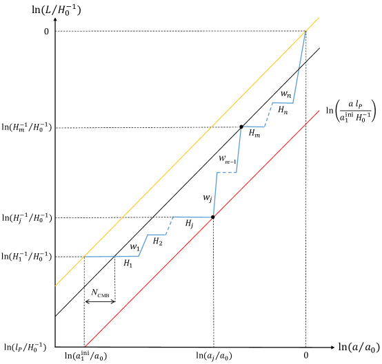
Figure 1: The sketch of multistage inflation confronted with the TCC. Here, $L\propto a$ denotes the physical length and $H_{0}$ is the Hubble parameter at present. The black line with slope equal to $1$ represents the evolution of the perturbation mode with the largest wavelength that can be observed at present. The red line represents the evolution of the perturbation mode with a physical wavelength equal to the Planck length at the beginning of the first inflationary stage. The blue polyline represents the evolution of the Hubble radius, where we have assumed that the $H_{i}$’s are almost constant during each stage of inflation and $w_{i}>-1/3$.

The logarithmic interval in comoving wave number of the perturbation modes that cross the horizon during a stage can be defined as

$$\tilde{N}=\Delta\ln k=\ln\left({a^{\text{end}}H^{\text{end}}\over a^{\text{ini}}H^{\text{ini}}}\right)\,,$$ (3)

where $k=aH$ is the comoving scale of the horizon size at time $t$. We also set the $e$-folding number $N=\ln\left({a^{\text{end}}\over a^{\text{ini}}}\right)$, and hence we have $\tilde{N}=N$ for $H^{\text{end}}=H^{\text{ini}}$. We use $\tilde{N}_{i}$ (or $N_{i}$) for the $i$th stage of inflation and $\tilde{N}_{w_{i}}$ (or $N_{w_{i}}$) for the $i$th stage of decelerated expansion with $w_{i}>-1/3$. Note that $\tilde{N}_{i}>0$ while $\tilde{N}_{w_{i}}<0$.

From Fig. 1, we have the following constraints on $\ln(H^{-1}/H_{0}^{-1})$.

Constraint 1: Perturbation modes with a wavelength equal to the Planck length at the beginning of the first stage of inflation will never cross the Hubble horizon. As a result, the red line [i.e., $\ln\left({al_{\text{P}}\over a_{1}^{\text{ini}}H_{0}^{-1}}\right)$] in Fig. 1 puts a lower bound on $\ln(H^{-1}/H_{0}^{-1})$, i.e.,

$${1\over aH}>{l_{\text{P}}\over a^{\text{min}}}\,,$$ (4)

where ”min” represents the minimum throughout the history of the Universe.

Constraint 2: Assuming that the first stage of inflation is responsible for the primordial perturbations in the CMB window, which should not be polluted by subsequent stages, we will have an upper bound (the black line in Fig. 1) on $\ln(H^{-1}/H_{0}^{-1})$, i.e.,

$${1\over aH}<{e^{-\tilde{N}_{\text{CMB}}}\over a_{1}^{\text{ini}}H_{1}^{\text{ini}}}\quad\text{for}\quad a_{1}^{\text{end}}<a<a_{\text{BB}}^{\text{ini}}\,,$$ (5)

where $\tilde{N}_{\text{CMB}}$ is the $e$-folding number of the CMB window, and $a_{\text{inf}}^{\text{end}}$ and $a_{\text{BB}}^{\text{ini}}$ are evaluated at the end of the first stage of inflation and the beginning of the hot BB expansion, respectively.

Considering multistage inflation with $n>1$ stages, for the $j$th stage, we can write down the bound (4) imposed by the TCC as

$$\tilde{N}_{j}+\sum_{i=1}^{j-1}(\tilde{N}_{i}+\tilde{N}_{w_{i}})=\ln\left({a_{j}^{\text{end}}H_{j}^{\text{end}}\over a_{1}^{\text{ini}}H_{1}^{\text{ini}}}\right)<\ln\left({M_{\text{P}}\over H_{1}^{\text{ini}}}\right)\,,$$ (6)

where we have used $\ln(a_{j}/a_{0})-\ln(a_{1}^{\text{ini}}/a_{0})<\ln(H_{j}^{-1}/H_{0}^{-1})-\ln(l_{\text{P}}/H_{0}^{-1})$ (note that slope of the red line in Fig. 1 is $1$) and $H_{1}^{\text{ini}}\simeq H_{1}^{\text{end}}$; see also Ref. [21]. We have set the Planck mass $M_{\text{P}}=l_{\text{P}}^{-1}$. Thus, for $n=1$, i.e., single-stage inflation, we have $\tilde{N}_{1}<\ln\left({M_{\text{P}}\over H_{1}^{\text{ini}}}\right)$ or equivalently $N_{1}<\ln\left({M_{\text{P}}\over H_{1}^{\text{end}}}\right)$, which is consistent with the result in Refs. [9, 10].

Based on Eqs. (5) and (6), for multistage inflation, the $j$th stage of inflation ($j\neq 1$) can be bounded as

$$\tilde{N}_{j}<\ln\left({M_{\text{P}}\over H_{1}^{\text{ini}}}\right)-\tilde{N}_{\text{CMB}}\,$$ (7)

for $a_{1}^{\text{end}}<a<a_{0}$. Therefore, the lifetime of the $j$th stage inflation is strictly bounded by the energy scale of the first stage of inflation and the width of the CMB window. Similarly, for a decelerated expanding stage, e.g., the stage marked by $w_{j-1}$, we have

$$-\tilde{N}_{w_{j-1}}={1\over 2}(1+3w_{j-1})N_{w_{j-1}}<\ln\left({M_{\text{P}}\over H_{1}^{\text{ini}}}\right)-\tilde{N}_{\text{CMB}}\,$$ (8)

for $a_{1}^{\text{end}}<a<a_{0}$. Note that $\tilde{N}_{w_{j-1}}<0$.

Therefore, if the TCC is correct and the first stage of inflation is responsible for the primordial perturbations in the CMB window, the $e$-folding number that the $j$th stage ($j\neq 1$, accelerated or decelerated) can last is bounded by the energy scale (or $H_{1}$) of the first stage of inflation; see also Ref. [21].

It is also possible that the perturbation modes of the present horizon scale $k_{0}=a_{0}H_{0}$ exit the horizon a few $e$-folds later than the beginning of the first stage of inflation. Furthermore, the CMB scale perturbation modes could even exit the horizon during the $i$th stage of inflation, where $i>1$, as long as these modes are deep inside the horizon before the $i$th stage [11]. In these situations, the bounds (4) and (6) still hold. However, since $a_{1}^{\text{ini}}H_{1}^{\text{ini}}$ is no longer the comoving wave number of the largest CMB scale perturbation modes, i.e., $k_{0}\neq a_{1}^{\text{ini}}H_{1}^{\text{ini}}$, the constraint (5) should be modified by replacing $a_{1}^{\text{ini}}H_{1}^{\text{ini}}$ with $k_{0}$. As a result, the bounds on $\tilde{N}_{j}$ and $\tilde{N}_{w_{j-1}}$ for $a_{i}^{\text{end}}<a<a_{0}$ will be tighter, since the right-hand sides of the bounds (7) and (8) should be corrected by subtracting the term $\ln\left({a_{0}H_{0}\over a_{1}^{\text{ini}}H_{1}^{\text{ini}}}\right)$. Hence, the inequalities (7) and (8) are still valid.

II.2 Multistage inflation in the AdS landscape

The landscape consists of all EFTs with a consistent UV completion, which might be from various compactifications of string theory. Otherwise, the set of corresponding EFTs is called the swampland. The distance conjecture $|\Delta\phi|/M_{\text{P}}<\Delta\sim{\cal O}(1)$ [5] and the dS conjecture $M_{\text{P}}|\nabla_{\phi}V|/V>c\sim{\cal O}(1)$ [6] [or the refined dS conjecture $M_{\text{P}}^{2}\frac{\text{min}\left(\nabla_{\phi}\nabla_{\phi}V\right)}{V}\leq-c^{\prime}\sim{\cal O}(1)$] [35, 34] have been proposed as the swampland criteria for EFTs. Recently, many efforts have been made to confront the inflation scenario with the swampland conjectures; see, e.g., Refs. [36, 37, 38, 39, 40, 41, 42, 43, 44].

The multistage inflation model (in which a high-scale inflation is followed by many low-scale inflations) might be interesting, since it helps to alleviate the bound of the TCC on the energy scale of inflation in the CMB window. Provided that the string landscape mostly consists of AdS vacua, we might have such a multistage inflation model; see Fig. 2(a). Each stage of slow-roll inflation only happened around the maxima of the potential barriers separated by AdS vacua ($\Delta\phi<M_{\text{P}}$ for each $V>0$ region). Between the $j$th and $(j+1)$th stages, the field will rapidly roll over an AdS vacuum.

As an illustrative example, we model the effective potential $V_{\text{eff}}(\phi)$ as

$$V_{\text{eff}}(\phi)=V_{0}\left(1-\cos\left(\frac{M}{\sqrt{V_{0}}}\phi\right)\right)e^{-\phi/\beta}-\Lambda,$$ (9)

which is similar to Fig. 2(a) (see also Ref. [48]), where $\Lambda=$ const $>0$ forces minima of the potential to be AdS, and $V_{0}$, $M$ and $\beta$ are positive constants that set the amplitude, period and envelope curve of $V_{\text{eff}}(\phi)$, respectively. The AdS potential (9) must satisfy the swampland distance conjecture as well as the de Sitter (or refined dS) conjecture. Considering that $1-\cos\left(\frac{M}{\sqrt{V_{0}}}\phi\right)=0$ and the AdS well has a width, we have $\Delta\phi<\frac{2\pi\sqrt{V_{0}}}{M}$ for $V(\phi)>0$. Hence, the swampland distance conjecture $|\Delta\phi|/M_{\text{P}}<{\cal O}(1)$ requires

$$\frac{\sqrt{V_{0}}}{M}<{\cal O}(1)\frac{M_{\text{P}}}{2\pi}\,.$$ (10)

Confronting the maxima of the potential (9) [at which $\cos\left(\frac{M}{\sqrt{V_{0}}}\phi\right)\approx-1$] with the refined de Sitter conjecture $M_{\text{P}}^{2}\frac{\text{min}\left(\nabla_{\phi}\nabla_{\phi}V\right)}{V}\leq-c^{\prime}\sim{\cal O}(1)$, we have

$$2V_{0}/\beta^{2}-M^{2}<-{\cal O}(1)\left({{2V_{0}-\Lambda}\over{M_{\text{P}}^{2}}}\right)\,.$$ (11)

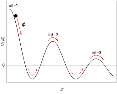
(a) $V(\Phi)$

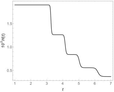
(b) $H(t)$

Figure 2: (a) Sketch of the AdS landscape. (b) The evolution of the Hubble parameter with the potential (9), in which $\Lambda=10^{-12}M_{\text{P}}^{4}$, $V_{0}=8*10^{-10}M_{\text{P}}^{4}$, $\beta=0.642M_{\text{P}}$ and $M=12\sqrt{V_{0}}M_{\text{P}}^{-1}$. These parameters satisfy the restrictions (10) and (11) of the swampland conjectures.

We will show the possibility of multistage inflation in an AdS landscape like Eq. (9). For simplicity, we assume that each stage of slow-roll inflation happens around one of the maxima of the potential (which is much larger than the depth of the AdS well, i.e., $V^{j}_{\text{inf}}\gg|\Lambda|$) and ends when the inflaton rolls rapidlly down the hill. When the $j$th stage of inflation ends, the potential energy $V_{\text{inf}}^{j}$ will be thoroughly converted to ${\dot{\phi}}^{2}$, so that the field can rapidly roll over an AdS well. During this era, which corresponds to $w_{j}\simeq 1$, we have $\dot{\phi}\sim a^{-3}$ and $\rho_{\phi}\approx\dot{\phi}^{2}/2\sim a^{-6}$. According to $3M_{\text{P}}^{2}H^{2}=\rho_{\phi}$, we get $\dot{\phi}\approx\sqrt{2/3}{M_{\text{P}}/t}$. Note that this result is valid only if ${\dot{\phi}}^{2}(t)\gg|\Lambda|$. After it rapidly rolls over the AdS well, the field must be able to slowly climb over the next maximum of the potential (${\dot{\phi}}^{2}\ll V_{\text{inf}}^{j+1}$), so that the $(j+1)$th stage of inflation can happen. During the period ${\dot{\phi}}^{2}\gg|V_{\text{eff}}|$, the shift of $\phi$ is approximately

$$\Delta\phi=\int_{t^{\text{ini}}}^{t^{\text{end}}}\dot{\phi}dt\approx\sqrt{2\over 3}M_{\text{P}}\ln\left({t^{\text{end}}\over t^{\text{ini}}}\right)\,.$$ (12)

Based on the above analysis, the ratio between the potential energy of the $(j+1)$th and $j$th stages of inflation is ${V_{\text{inf}}^{j+1}/V_{\text{inf}}^{j}}\approx\left({\dot{\phi}^{\text{end}}/\dot{\phi}^{\text{ini}}}\right)^{2}\approx\left({t^{\text{ini}}/t^{\text{end}}}\right)^{2}$. Using Eq. (12), we find

$${V_{\text{inf}}^{j+1}\over V_{\text{inf}}^{j}}\approx\exp\left(-\sqrt{6}{\Delta\phi\over M_{\text{P}}}\right)\,.$$ (13)

Therefore, the AdS landscape (9) is viable for multistage inflation. Actually, from (9) and (13) we find $\beta\approx{\cal O}(M_{\text{P}}/\sqrt{6})\approx{\cal O}(0.4M_{\text{P}})$. However, it can be inferred that the value of $\beta$ is fine-tuned so that the inflaton does not overshoot the potential maxima at a large velocity or become trapped in the AdS vacuum. The numerical calculation hints that there exists an amount of parameter fine-tuning at least of order $10^{-2}M_{\text{P}}$ for $\beta$ to prevent both things from happening. How to alleviate the fine-tuning in a realistic multistage inflation model requires further investigation.

Here, as an example, we plot the evolution of the background (the Hubble parameter) with the AdS potential (9) in Fig. 2(b), which is clearly multistage inflation. The parameters $V_{0}$, $M$, $\beta$, and $\Lambda$ used in Fig. 2(b) satisfy the bounds (10) and (11). Here we have assumed $V^{i}_{\text{inf}}\gg|\Lambda|$, and thus the ratio ${H_{\text{inf}}^{j+1}/H_{\text{inf}}^{j}}$ is small. Generally, the AdS minima have different values. Consequently, we may not have $V^{i}_{\text{inf}}\gg|\Lambda|$ for each $V^{i}_{\text{inf}}$, which will result in a larger ${H_{\text{inf}}^{j+1}/H_{\text{inf}}^{j}}$.

III Implications for Dark Energy

The Universe is currently in an accelerated phase of expansion. Nearly $70$% of the Universe is made up of dark energy (DE) [49] and its equation-of-state parameter is approximately $w\simeq-1$. Thus, this accelerated stage of expansion has similar behavior as primordial inflation, which hence may be thought of as one stage of a multistage inflation scenario, see Fig. 3. According to Sec. II.1, the TCC will put a bound on the lifetime of the DE era.

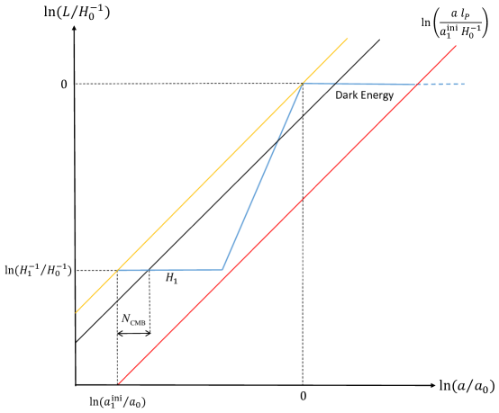
Figure 3: Sketch of the dark energy era confronted with the TCC.

For simplicity, we assume that after the first stage of inflation ($H_{1}=H_{\text{inf}}$) the Universe experiences the hot BB evolution up to the present DE era (the second stage of inflation, $H_{2}=H_{\text{DE}}$). Thus setting $j=2$ in Eq. (6), the TCC bound on the DE era is

$$\tilde{N}_{\text{DE}}<\ln\left({M_{\text{P}}\over H_{\text{inf}}^{\text{ini}}}\right)\,,$$ (14)

since $\tilde{N}_{w_{1}}=-\tilde{N}_{1}$. Here we do not need to make allowance for the CMB window, which actually corresponds to setting $a_{\text{DE}}^{\text{ini}}H_{\text{DE}}^{\text{ini}}\approx a_{\text{inf}}^{\text{ini}}H_{\text{inf}}^{\text{ini}}$. Therefore, if $H_{\text{DE}}=H_{0}$ is approximately constant, the lifetime of the current DE era is

$$\Delta t<{1\over H_{0}}\ln\left({M_{\text{P}}\over H_{\text{inf}}^{\text{end}}}\right),$$ (15)

which is far smaller than the expected value ${1\over H_{0}}\ln({M_{\text{P}}\over H_{0}})$, since $H_{\text{inf}}^{\text{end}}\gg H_{0}$ (even if $H_{\text{inf}}^{\text{end}}$ is reduced to $\sim 0.1$ GeV [10]). Intriguingly, if the TCC is correct, it seems that the fate of our Universe is fixed by the properties of primordial inflation, rather than DE itself.

It should be mentioned that we have assumed that the present horizon scale $k_{0}$ is the same as the horizon size at the beginning of inflation, i.e., $k_{0}=a_{0}H_{0}=a_{\text{inf}}^{\text{ini}}H_{\text{inf}}^{\text{ini}}$. If the perturbation mode with comoving wave number $k_{0}$ exits the horizon a few $e$-folds after the beginning of inflation, then the bounds on $\tilde{N}_{\text{DE}}$ and $\Delta t$ will be tighter, since the right-hand sides of Eqs. (14) and (15) should be subtracted by terms $\ln\left({a_{\text{DE}}^{\text{ini}}H_{\text{DE}}^{\text{ini}}\over a_{\text{inf}}^{\text{ini}}H_{\text{inf}}^{\text{ini}}}\right)$ and ${1\over H_{0}}\ln\left({a_{\text{DE}}^{\text{ini}}H_{\text{DE}}^{\text{ini}}\over a_{\text{inf}}^{\text{ini}}H_{\text{inf}}^{\text{ini}}}\right)$, respectively. Therefore, the bounds (14) and (15) are still valid in this situation, but the actual allowed lifetime of the DE era should be shorter for an amount of ${1\over H_{0}}\ln\left({a_{\text{DE}}^{\text{ini}}H_{\text{DE}}^{\text{ini}}\over a_{\text{inf}}^{\text{ini}}H_{\text{inf}}^{\text{ini}}}\right)$ than that estimated from Eq. (15).

It is also possible that alternative models of inflation could be the origin of primordial perturbations that are consistent with observations (e.g., Refs. [50, 51, 52, 53, 54]). It would be interesting to see what would happen to $\tilde{N}_{\text{DE}}$ with these alternatives. Considering a nonsingular bouncing scenario, we have $a^{\text{min}}=a_{\text{b}}$, where $a_{\text{b}}$ is evaluated at the bounce point. According to Eq. (4), assuming that the Universe will start to hot-BB-like expand immediately after the bounce (i.e., $a_{\text{b}}\approx a_{\text{BB}}^{\text{ini}}$), we have

$$\tilde{N}_{\text{DE}}<\ln\left({a_{\text{b}}/l_{\text{P}}\over a_{\text{DE}}^{\text{ini}}H_{\text{DE}}^{\text{ini}}}\right)\approx\left|\tilde{N}_{\text{BB}}\right|+\ln\left({M_{\text{P}}\over H_{\text{BB}}^{\text{ini}}}\right)\,,$$ (16)

where $\tilde{N}_{\text{BB}}=\ln\left({a_{\text{DE}}^{\text{ini}}H_{\text{DE}}^{\text{ini}}\over a_{\text{BB}}^{\text{ini}}H_{\text{BB}}^{\text{ini}}}\right)<0$ is the logarithmic interval in comoving wave number of the perturbation modes entering the horizon during the hot BB evolution before the DE era. Here, Eq. (16) is applicable whether we assume an ekpyrosis [50] or matter bounce [51] scenario. Also, for the slow-expansion scenario (in which the expansion is ultra-slow with $\epsilon=-{\dot{H}}/H^{2}\ll-1$ before the hot BB evolution) [53, 54] the result is similar.

Therefore, if the Universe rapidly reheated after the end of inflation or its alternatives, such that $H^{\text{end}}_{\text{inf}}=H_{\text{BB}}^{\text{ini}}$, and also experienced the same hot BB expansion, the DE era in the inflation scenario would be much shorter than that in alternatives to inflation. This is because the TCC bound on inflation is much tighter than that on its alternatives, as pointed out in Ref. [10]. Interestingly, if the TCC is correct, the lifetime of the DE era might be a probe for distinguishing different possibilities for the origins of the Universe.

IV Discussion

As one possible criteria for consistent EFTs, the TCC sets an upper bound on the energy scale of inflation, which renders $r$ in the CMB window negligibly small. Recently, the implications of the TCC for inflation have inspired studies of multistage inflation.

We showed that if the TCC is correct and the first stage of inflation is responsible for the primordial perturbations in the CMB window, the $e$-folding number of the $j$th stage ($j\neq 1$) will be bounded by the energy scale of the first stage of inflation. Regarding the DE era as one stage of a multistage inflation scenario, we pointed out that in the inflation scenario the lifetime of the current DE era is far smaller than expected, which might be a probe for distinguishing inflation from its alternatives. Our result may also place constraints on EFTs of DE, which would be an interesting topic for future work.

By assuming that the landscape of EFTs consists mostly of AdS vacua, we presented a multistage inflation model in the AdS landscape (with AdS vacua separated by barriers $V>0$). Each inflationary stage only happens around the maxima of the potential barriers. The field will rapidly roll over an AdS vacuum between two stages. Such a model naturally satisfies all swampland conjectures. Note that the AdS potential is also present in past-complete pre-inflation stages [11]. Thus, if the TCC is correct, the issues related to the early Universe and DE (especially in the AdS landscape) would be worthy of further exploration.

References

- [1] A. H. Guth, Phys. Rev. D 23, 347 (1981).
- [2] A. A. Starobinsky, Phys. Lett. 91B, 99 (1980).
- [3] A. D. Linde, Phys. Lett. 108B, 389 (1982).
- [4] A. Albrecht and P. J. Steinhardt, Phys. Rev. Lett. 48, 1220 (1982).
- [5] H. Ooguri and C. Vafa, Nucl. Phys. B766, 21 (2007).
- [6] G. Obied, H. Ooguri, L. Spodyneiko and C. Vafa, arXiv:1806.08362.
- [7] R. H. Brandenberger and J. Martin, Mod. Phys. Lett. A 16, 999 (2001).
- [8] J. Martin and R. H. Brandenberger, Phys. Rev. D 63, 123501 (2001).
- [9] A. Bedroya and C. Vafa, arXiv:1909.11063.
- [10] A. Bedroya, R. Brandenberger, M. Loverde and C. Vafa, arXiv:1909.11106.
- [11] Y. Cai and Y. S. Piao, arXiv:1909.12719.
- [12] T. Tenkanen, arXiv:1910.00521.
- [13] S. Das, Phys. Dark Univ. 27, 100432 (2020).
- [14] S. Mizuno, S. Mukohyama, S. Pi, and Y. L. Zhang, arXiv:1910.02979.
- [15] S. Brahma, Phys. Rev. D 101, no. 2, 023526 (2020).
- [16] M. Dhuria and G. Goswami, Phys. Rev. D 100, no. 12, 123518 (2019).
- [17] M. Torabian, Fortsch. Phys. 68, no. 2, 1900092 (2020).
- [18] R. G. Cai and S. J. Wang, Phys. Rev. D 101, no. 4, 043508 (2020).
- [19] K. Schmitz, Phys. Lett. B 803, 135317 (2020).
- [20] K. Kadota, C. S. Shin, T. Terada, and G. Tumurtushaa, J. Cosmol. Astropart. Phys. 01 (2020) 008.
- [21] A. Berera and J. R. Calderón, Phys. Rev. D 100, no. 12, 123530 (2019).
- [22] S. Brahma, Phys. Rev. D 101, no. 4, 046013 (2020).
- [23] N. Okada, D. Raut, and Q. Shafi, arXiv:1910.14586.
- [24] S. Laliberte and R. Brandenberger, arXiv:1911.00199.
- [25] G. Goswami and C. Krishnan, arXiv:1911.00323.
- [26] W. C. Lin and W. H. Kinney, arXiv:1911.03736.
- [27] G. Dvali and S. Kachru, in From Fields to String, edited by M. Shifman et al., vol. 2, pp.1131-1155.
- [28] C. P. Burgess, R. Easther, A. Mazumdar, D. F. Mota, and T. Multamaki, J. High Energy Phys. 05 (2005) 067.
- [29] Y. Liu, Y. S. Piao, and Z. G. Si, J. Cosmol. Astropart. Phys. 05 (2009) 008.
- [30] M. Li and Y. Wang, J. Cosmol. Astropart. Phys. 07 (2009) 033.
- [31] S. Li, Y. Liu, and Y. S. Piao, Phys. Rev. D 80, 123535 (2009).
- [32] Y. Wang, arXiv:1001.0008.
- [33] N. Afshordi, A. Slosar, and Y. Wang, J. Cosmol. Astropart. Phys. 01 (2011) 019.
- [34] S. K. Garg and C. Krishnan, J. High Energy Phys. 11 (2019) 075.
- [35] H. Ooguri, E. Palti, G. Shiu, and C. Vafa, Phys. Lett. B 788, 180 (2019).
- [36] A. Achucarro and G. A. Palma, J. Cosmol. Astropart. Phys. 02 (2019) 041.
- [37] A. Kehagias and A. Riotto, Fortsch. Phys. 66, 1800052 (2018).
- [38] H. Matsui and F. Takahashi, Phys. Rev. D 99, 023533 (2019).
- [39] W. H. Kinney, S. Vagnozzi, and L. Visinelli, Classical Quantum Gravity 36, 117001 (2019).
- [40] S. Brahma and M. Wali Hossain, J. High Energy Phys. 03 (2009) 006.
- [41] M. Motaharfar, V. Kamali, and R. O. Ramos, Phys. Rev. D 99, 063513 (2019).
- [42] A. Ashoorioon, Phys. Lett. B 790, 568 (2019).
- [43] S. Das, Phys. Rev. D 99, 063514 (2019).
- [44] W. H. Kinney, Phys. Rev. Lett. 122, 081302 (2019).
- [45] V. N. Senoguz and Q. Shafi, Phys. Lett. B 596, 8 (2004).
- [46] L. Boubekeur and D. H. Lyth, J. Cosmol. Astropart. Phys. 07 (2005) 010.
- [47] K. Kohri, C. M. Lin, and D. H. Lyth, J. Cosmol. Astropart. Phys. 12 (2007) 004.
- [48] Y. S. Piao, Phys. Rev. D 70, 101302 (2004).
- [49] N. Aghanim et al. (Planck Collaboration), arXiv:1807.06209.
- [50] J. Khoury, B. A. Ovrut, P. J. Steinhardt, and N. Turok, Phys. Rev. D 64, 123522 (2001).
- [51] F. Finelli and R. Brandenberger, Phys. Rev. D 65, 103522 (2002); D. Wands, Phys. Rev. D 60, 023507 (1999).
- [52] R. H. Brandenberger and C. Vafa, Nucl. Phys.B316, 391 (1989); A. Nayeri, R. H. Brandenberger, and C. Vafa, Phys. Rev. Lett. 97, 021302 (2006).
- [53] Y. S. Piao and E. Zhou, Phys. Rev. D 68, 083515 (2003); Z. G. Liu, J. Zhang and Y. S. Piao, Phys. Rev. D 84, 063508 (2011).
- [54] P. Creminelli, A. Nicolis, and E. Trincherini, J. Cosmol. Astropart. Phys. 11 (2010) 021.